Ab-initio Theory of Photoionization via Resonances

Abstract

We present an ab-initio approach for computing the photoionization spectrum near autoionization resonances in multi-electron systems. While traditional (Hermitian) theories typically require computing the continuum states, which are difficult to obtain with high accuracy, our non-Hermitian approach requires only discrete bound and metastable states, which can be accurately computed with available quantum chemistry tools. We derive a simple formula for the absorption lineshape near Fano resonances, which relates the asymmetry of the spectral peaks to the phase of the complex transition dipole moment. Additionally, we present a formula for the ionization spectrum of laser-driven targets and relate the “Autler-Townes” splitting of spectral lines to the existence of exceptional points in the Hamiltonian. We apply our formulas to compute the autoionization spectrum of helium, but our theory is also applicable for non-trivial multi-electron atoms and molecules.

We present an ab-initio approach for computing the photoionization spectrum near autoionization (AI) resonances in multi-electron systems. Recent developments in attosecond-laser technology enable probing and controlling photoionization processes, and lead to a renewed interest in ionization and related phenomena, such as high-harmonic generation and strong-field electronic dynamics Krausz and Ivanov (2009); Itatani et al. (2004); Paul et al. (2001); Klünder et al. (2011); Azoury et al. (2017). These experimental capabilities call for ab-initio theories, which can relate the electronic structure of the sampled medium to the measured ionization spectrum. However, most existing theories require the calculation of the continuum states Feshbach (1962); Friedrich and Wintgen (1985) (above the ionization threshold), which are difficult to obtain with high accuracy with traditional methods Averbukh and Cederbaum (2005); Goetz et al. (2017). In this work, we use non-Hermitian quantum mechanics (NHQM) Moiseyev (2011) in order to avoid the need of computing continuum states. Our theory produces a simple formula for the “Fano asymmetry parameter” [Eq. (32)], which expresses the asymmetry of the peaks in the ionization spectrum near AI resonances Fano (1961), and a formula for the photoionization spectrum of laser-driven systems [Eq. (34)]. We relate the Autler-Townes Autler and Townes (1955) splitting of ionization spectral peaks to the existence of exceptional points Kato (2013) (EPs)—special degenerate resonances where multiple AI states share the same energy and wavefunction. We demonstrate the predictions of our theory for helium using ab-initio electronic-structure data from Kaprálová-Žďánská, Šmydke, and Civiš (2013); Kaprálová-Žďánská and Šmydke (2013). By using advanced non-Hermitian quantum-chemistry algorithms Zuev et al. (2014); Landau et al. (2016), our theory can also be applied for larger atoms and molecules.

In NHQM, the time-independent Schrödinger equation is solved with outgoing boundary conditions and the resulting energy spectrum is discrete, containing real-energy bound states and complex-energy metastable states Moiseyev (2011). This situation is very different from traditional Hermitian quantum mechanics (HQM), where metastable (autoionizing) states are described as real-energy bound states embedded in a continuum of free states Fano (1961). Moreover, in HQM, the transition dipole moment is real, while in NHQM, it is generally complex. We show that the phase of the complex transition dipole moment has physical significance: it determines the asymmetry of the absorption peaks near AI states (see Fig. 1). Our derivation of the Fano asymmetry parameter is inspired by the recent work of Fukuta et al. Fukuta et al. (2017), which used a non-Hermitian approach to compute the Fano factor, although Fukuta et al. (2017) introduced an artificial model for the continuum and did not relate the lineshape to the complex transition dipole moment.

As an application of our approach, we study the suppression and enhancement of photoionization in the presence of an external driving laser [Fig. 2]—two effects which are closely related to electromagnetically induced transparency (EIT) Boller, Imamoğlu, and Harris (1991); Harris, Field, and Imamoğlu (1990); Harris (1997); Fleischhauer and Lukin (2000); Fleischhauer, Imamoglu, and Marangos (2005) and absorption (EIA) Lezama, Barreiro, and Akulshin (1999); Goren et al. (2003); Zhang et al. (2015). Laser-induced suppression of photoionization was first measured in magnesium Karapanagioti et al. (1995, 1996), and later demonstrated in several other systems Halfmann et al. (1998); Gao et al. (2000). These experiments were modeled using the Feshbach formalism Bachau, Lambropoulos, and Shakeshaft (1986); Karapanagioti et al. (1996), which requires the computation of the continuum states and can be avoided by our approach. Motivated by the huge impact of EIT in optics and atomic physics Harris, Field, and Imamoğlu (1990); Harris (1997); Fleischhauer and Lukin (2000); Fleischhauer, Imamoglu, and Marangos (2005), we believe that the ability to accurately compute the analogous effects for AI states will open new routes for controlling and understanding photoionization and related phenomena (e.g., photoassociation and photodetachment).

We begin by reviewing the traditional theory of photoionization Fano (1961). In order to obtain the photoionization spectrum, one needs to compute the rate at which an absorbed photon excites an atom (or molecule) into an AI state. The transition rate induced by a linearly polarized electromagnetic field (with frequency $\omega$, amplitude $\mathcal{E}$, and polarization axis $\hat{x}$) can be computed using Fermi’s golden rule Yan and Mukamel (1986)

$$S(\omega)=\frac{|\mathcal{E}|^{2}}{\hbar}\operatorname*{\mathchoice{\ooalign{$\displaystyle\sum$\cr$\displaystyle\int$\cr}}{\ooalign{\raisebox{0.14pt}{\scalebox{0.75}{$\displaystyle\sum$}}\cr{\scalebox{0.75}{$\displaystyle\int$}}\cr}}{\ooalign{\raisebox{0.2pt}{\scalebox{0.6}{$\scriptstyle\sum$}}\cr$\scriptstyle\int$\cr}}{\ooalign{\raisebox{0.2pt}{\scalebox{0.6}{$\scriptstyle\sum$}}\cr$\scriptstyle\int$\cr}}}_{f}\left|\langle{\phi_{i}}|x|{\phi_{f}}\rangle\right|^{2}\delta(\hbar\omega-\varepsilon_{f}+\varepsilon_{i}).$$ (9)

Here, $\varepsilon_{i,f}$ and $|{\phi_{i,f}}\rangle$ are the initial- and final-state energies and wavefunctions respectively, while $\operatorname*{\mathchoice{\ooalign{$\displaystyle\sum$\cr$\displaystyle\int$\cr}}{\ooalign{\raisebox{0.14pt}{\scalebox{0.75}{$\displaystyle\sum$}}\cr{\scalebox{0.75}{$\displaystyle\int$}}\cr}}{\ooalign{\raisebox{0.2pt}{\scalebox{0.6}{$\scriptstyle\sum$}}\cr$\scriptstyle\int$\cr}}{\ooalign{\raisebox{0.2pt}{\scalebox{0.6}{$\scriptstyle\sum$}}\cr$\scriptstyle\int$\cr}}}_{f}$ denotes summation over bound and integration over continuum final states. The eigenfunctions and energies are obtained by diagonalizing the Hamiltonian (e.g., by using standard quantum-chemistry tools Schmidt et al. (1993)). Since the continuum states have delocalized wavefunctions, it is challenging to compute them with the same level of accuracy as the bound states Averbukh and Cederbaum (2005); Goetz et al. (2017).

This difficulty can be circumvented by using the Green’s function eigenstate-free method (developed in Refs. 34; 32). In this approach, one first decomposes the Hamiltonian of the system into the “initial- and excited-state Hamiltonians,” defined as $\mathbb{H}_{i}\equiv\varepsilon_{i}|{\phi_{i}}\rangle\langle{\phi_{i}}|$ and $\mathbb{H}_{\mathrm{exc}}\equiv\operatorname*{\mathchoice{\ooalign{$\displaystyle\sum$\cr$\displaystyle\int$\cr}}{\ooalign{\raisebox{0.14pt}{\scalebox{0.75}{$\displaystyle\sum$}}\cr{\scalebox{0.75}{$\displaystyle\int$}}\cr}}{\ooalign{\raisebox{0.2pt}{\scalebox{0.6}{$\scriptstyle\sum$}}\cr$\scriptstyle\int$\cr}}{\ooalign{\raisebox{0.2pt}{\scalebox{0.6}{$\scriptstyle\sum$}}\cr$\scriptstyle\int$\cr}}}_{f}\varepsilon_{f}|{\phi_{f}}\rangle\langle{\phi_{f}}|$ respectively. The key idea of this approach is to realize that the summation in Eq. (9) can be avoided by exploiting the “excited-states’ Green’s function,” which is the impulse response of the operator $\mathbb{H}_{\mathrm{exc}}$, defined as Trefethen and Bau III (1997)

$$\mathbb{G}_{\mathrm{exc}}(\varepsilon)\equiv(\mathbb{H}_{\mathrm{exc}}-\varepsilon)^{-1}=\operatorname*{\mathchoice{\ooalign{$\displaystyle\sum$\cr$\displaystyle\int$\cr}}{\ooalign{\raisebox{0.14pt}{\scalebox{0.75}{$\displaystyle\sum$}}\cr{\scalebox{0.75}{$\displaystyle\int$}}\cr}}{\ooalign{\raisebox{0.2pt}{\scalebox{0.6}{$\scriptstyle\sum$}}\cr$\scriptstyle\int$\cr}}{\ooalign{\raisebox{0.2pt}{\scalebox{0.6}{$\scriptstyle\sum$}}\cr$\scriptstyle\int$\cr}}}_{f}\frac{|{\phi_{f}}\rangle\langle{\phi_{f}}|}{\langle{\phi_{f}}|{\phi_{f}}\rangle}\frac{1}{\varepsilon-\varepsilon_{f}}.$$ (18)

In the second equality, we employ the normal-mode expansion of the Green’s function Arfken and Weber (2006) . Using a mathematical identity for the $\delta$-function Shibatani and Toyozawa (1968), one can rewrite Eq. (9) as

$$S(\omega)=\operatorname*{\mathchoice{\ooalign{$\displaystyle\sum$\cr$\displaystyle\int$\cr}}{\ooalign{\raisebox{0.14pt}{\scalebox{0.75}{$\displaystyle\sum$}}\cr{\scalebox{0.75}{$\displaystyle\int$}}\cr}}{\ooalign{\raisebox{0.2pt}{\scalebox{0.6}{$\scriptstyle\sum$}}\cr$\scriptstyle\int$\cr}}{\ooalign{\raisebox{0.2pt}{\scalebox{0.6}{$\scriptstyle\sum$}}\cr$\scriptstyle\int$\cr}}}_{f}\langle{\phi_{i}}|x|{\phi_{f}}\rangle\left(\tfrac{1}{\hbar\pi}\mathrm{Im}\!\lim_{s\rightarrow 0^{+}}\tfrac{|\mathcal{E}|^{2}}{\hbar\omega-is-\varepsilon_{f}+\varepsilon_{i}}\right)\langle{\phi_{f}}|x|{\phi_{i}}\rangle,$$ (27)

where the modes are normalized to one (i.e., $\langle{\phi_{f}}|{\phi_{f}}\rangle=1$). Then, by substituting Eq. (18) into Eq. (27), one obtains

$$S(\omega)=\frac{|\mathcal{E}|^{2}}{\hbar\pi}\mathrm{Im}\langle{\phi_{i}}|x\,\,\mathbb{G}_{\mathrm{exc}}\,x|{\phi_{i}}\rangle,$$ (28)

where $\mathbb{G}_{\mathrm{exc}}(\varepsilon)$ is evaluated at $\varepsilon=\hbar\omega+\varepsilon_{i}$.

Although Eq. (28) does not contain summation over continuum states [and is, therefore, more efficient than Eq. (9) in many cases], obtaining the excited-state Green’s function of multi-electron systems requires significant computation power. However, the Green’s function formulation naturally extends to NHQM, which offers a huge computational advantage. Under the conditions stated below, one can replace the Hermitan normal-mode expansion of $G_{\mathrm{exc}}$ [Eq. (18)] with the non-Hermitian quasi-normal mode expansion Moiseyev (2011); Trefethen and Embree (2005):

$$G_{\mathrm{exc}}(\varepsilon)=\sum_{f}\frac{|{\phi^{R}_{f}})({\phi_{f}^{L}}|}{({\phi_{f}^{L}}|{\phi_{f}^{R}})}\frac{1}{\varepsilon-\varepsilon_{f}}.$$ (29)

Here, $|{\phi_{f}^{R}})$ and $\varepsilon_{f}$ are the discrete eigenvectors and eigenvalues of the (non-Hermitian) time-independent Schrödinger equation—solved with outgoing boundary conditions—and $|{\phi_{f}^{L}})$ are the eigenvectors of the transposed Schrödinger equation. Round brackets denote the “unconjugated norm:” $({\phi}|{\psi})\equiv\int\!dx\,\phi\psi$ Moiseyev (2011), which generalizes the traditional Dirac “conjugated norm,” $\langle\phi|\psi\rangle\equiv\int\!dx\,\phi^{*}\psi$ Griffiths (2005) from HQM. Since the energy spectrum in NHQM is discrete, we replace $\operatorname*{\mathchoice{\ooalign{$\displaystyle\sum$\cr$\displaystyle\int$\cr}}{\ooalign{\raisebox{0.14pt}{\scalebox{0.75}{$\displaystyle\sum$}}\cr{\scalebox{0.75}{$\displaystyle\int$}}\cr}}{\ooalign{\raisebox{0.2pt}{\scalebox{0.6}{$\scriptstyle\sum$}}\cr$\scriptstyle\int$\cr}}{\ooalign{\raisebox{0.2pt}{\scalebox{0.6}{$\scriptstyle\sum$}}\cr$\scriptstyle\int$\cr}}}$ by $\sum$.

Equation 29 is valid assuming that ($i$) the Green’s function is evaluated near the resonant energies (i.e., when $\varepsilon\approx\mathrm{Re}[\varepsilon_{f}]$), ($ii$) the excited AI states, ${\phi^{R}_{f}}(x)$, are evaluated near the interaction region Lee, Leung, and Pang (1999); Leung, Liu, and Young (1994) (i.e., not far from the atomic core, $|x|\approx a_{0}$, where $a_{0}$ is the Bohr radius), and ($iii$) when the energy spectrum does not contain EPs. Condition ($i$) is satisfied (in all cases of interest) since we apply Eq. (29) only to study resonant absorption. Condition ($ii$) is fulfilled because the absorption formula [Eq. (28)] depends only on the overlap integral between extended AI states, ${\phi^{R}_{f}}(x)$, and localized bound states, ${\phi^{R}_{i}}(x)$. Although the eigenvectors of the non-Hermitian Hamiltonian, ${\phi^{R}_{f}}(x)$, are typically poor approximations for the “physical” metastable-state wavefunctions far from the interaction region (where they have diverging tails Moiseyev (2011)), their unphysical values at large distances do not contribute to the absorption spectrum since the bound-state wavefunctions vanish at large distances. Last, when the energy spectrum contains EPs, Eq. (29) breaks down because the quasi-normal modes, ${\phi^{R}_{f}}(x)$, do not form a complete basis of the Hilbert space Hanson, Nosich, and Kartchevski (2003); Hernandez, Jauregui, and Mondragon (2000); Hernàndez and Mondragòn (2003); Pick et al. (2017). At an EP, the “unconjugated norm” of the degenerate state, $({\phi_{\mathrm{EP}}^{L}}|{\phi_{\mathrm{EP}}^{R}})$, vanishes and the associated term in Eq. (29) blows up. One can obtain a corrected formula for $G_{\mathrm{exc}}$ at the EP by considering Eq. (29) near the EP and carefully taking the limit of approaching the EP. In this limit, the two terms in the sum that are associated with the nearly degenerate poles dominate the impulse response due to their infinitesimal denominators. However, one finds that two terms diverge with opposite signs, while their sum remains finite. This point was previously realized on pure mathematical grounds Trefethen and Embree (2005), and later explained in the context of electromagnetic modes Hanson, Nosich, and Kartchevski (2003); Hernandez, Jauregui, and Mondragon (2000); Hernàndez and Mondragòn (2003); Pick et al. (2017). We sketch the derivation of the corrected formula for $G_{\mathrm{exc}}$ in the context of AI states in the supporting information (SI) appendix.

By substituting Eq. (29) into Eq. (28), we obtain the NHQM absorption spectrum formula:

$$S(\omega)=\frac{\left|\mathcal{E}\right|^{2}}{\hbar\pi}\mathrm{Im}\sum_{f}\frac{({\phi_{i}^{L}}|x|{\phi_{f}^{R}})({\phi_{f}^{L}}|x|{\phi_{i}^{R}})}{({\phi_{f}^{L}}|{\phi_{f}^{R}})(\hbar\omega-\varepsilon_{f}+\varepsilon_{i})}.$$ (30)

This formula applies to cases where the initial state is bound and, therefore, one can replace Dirac bracket states, $|\phi_{i}\rangle$ and $\langle\phi_{i}|$, with unconjugated bracket states $|{\phi_{i}^{R}})$ and $({\phi_{i}^{L}}|$ (since the left eigenvector of a Hermitian Hamiltonian is equal to the conjugated right eigenvector of the same eigenvalue ). However, when the initial state is metastable, one needs to keep the conjugated bracket for the initial state. Our derivation of Eq. (30) is similar in spirit to the recent work of Fukuta et al. Fukuta et al. (2017), which used NHQM to compute the absorption spectrum. However, the latter work introduced an artificial model for the continuum (which limits its generality) and did not relate the spectrum directly to the complex transition dipole moment.

Equation 30 applies both for autoionizing atoms and molecules. In either case, the AI rate depends on the complex transition moment between initial and final states of the system. While in atoms, ionizing transitions involve two different electronic states, in molecules (where the wavefunction depends both on electronic and nuclear coordinates), there are, generally speaking, two possibilities: ($i$) Either the initial and final electronic states are different but the nuclear rovibrational state is the same (as in penning ionization Penning (1927); Miller (1970); Henson et al. (2012); Bhattacharya et al. (2017) or interatomic Coulombic decay Cederbaum, Zobeley, and Tarantelli (1997); Santra et al. (2000); Averbukh, Müller, and Cederbaum (2004)) or ($ii$) the initial and final electronic states are the same but the nuclear rovibrational state is different (as in dipole-bound anions Edwards, Johnson, and Tully (2012) or intermolecular vibrational-energy transfer Cederbaum (2018)). In case ($i$) (which involves transitions between different electronic state), ionization can occur provided that the energy of the excited electronic state exceeds the ground-state energy of the ion (i.e., the ionization threshold); under this condition, the excited state is degenerate with the continuum of free electronic states. Such processes are accurately described within the Born–Oppenheimer (BO) approximation, which amounts to assuming that the motion of atomic nuclei and electrons in a molecule can be separated Levine (2000). In case ($ii$) (which involves different nuclear rovibrational states), ionization happens due to non-adiabatic coupling terms (i.e., corrections beyond the BO approximation), which provide coupling between the electronic states of the molecule in different nuclear configuration. In order for AI to occur in such cases, the rovibrational energy must exceed the binding energy of the electron to the molecule. While the latter situation has been treated in Edwards, Johnson, and Tully (2012), our new formula [Eq. (30)] applies to all cases. Note that Edwards, Johnson, and Tully (2012) uses Hermitian scattering theory, while our approach uses NHQM, which makes the spectrum discrete and, therefore, produces a computationally efficient formula.

Our non-Hermitian formula [Eq. (30)] provides a simple formula for the “Fano asymmetry parameter,” which expresses the asymmetry of the peaks in the ionization spectrum near AI resonances Fano (1961). According to traditional absorption theory Fano (1961); Shibatani and Toyozawa (1968), the spectrum near an isolated resonance with frequency $\Omega$ and lifetime $1/\gamma$ can be written as

$$S_{\mathrm{F}}(\omega)=S_{0}(\omega)\,\frac{(\omega-\Omega+\tfrac{\gamma}{2}q)^{2}}{(\omega-\Omega)^{2}+(\tfrac{\gamma}{2})^{2}},$$ (31)

where $S_{0}(\omega)$ is the background absorption due to continuum states and the remaining expression is the resonant peak. The parameter $q$ determines the asymmetry of the resonant peak: in the limit of $q\rightarrow\infty$, the lineshape is Lorentzian, while the limit of $q\simeq 1$ produces an asymmetric lineshape. In traditional HQM, $q$ is found by computing overlap integrals involving bound and continuum states Fano (1961); Shibatani and Toyozawa (1968). In our approach, however, the $q$ factor depends on a single term in Eq. (30) (for which $\mathrm{Re}[\varepsilon_{f}-\varepsilon_{i}]\approx\hbar\Omega$). By taking the ratio of the symmetric and anti-symmetric parts of that term (similar to Fukuta et al. (2017)), we obtain the compact expression

$$q=\left|\frac{\mathrm{Re}\,\mu_{if}^{2}}{\mathrm{Im}\,\mu_{if}^{2}}\right|\left[1\pm\sqrt{1+\left(\tfrac{\mathrm{Im}\,\mu_{if}^{2}}{\mathrm{Re}\,\mu_{if}^{2}}\right)^{2}}\right],$$ (32)

where we introduced a shorthand notation for the squared transition dipole moment, $\mu_{if}^{2}\equiv({\phi_{i}^{L}}|x|{\phi_{f}^{R}})({\phi_{f}^{L}}|x|{\phi_{i}^{R}})$. The sign of $q$ indicates whether the absorption peak is blue or red shifted, and is determined by the sign of $\mathrm{Im}\,\mu_{ij}^{2}$. More details on the derivation are given in the SI. Our formula for $q$ generalizes an earlier result from Edwards, Johnson, and Tully (2012), which analyzed molecular photodetachment. The formulas agree qualitatively in the limit of large $q$, which corresponds to nearly Lorentzian AI peaks. While in our case, this limit is attained for nearly real resonant energies, $\varepsilon_{f}$ (which are associated with nearly real transition dipole moments, $\mu_{ij}$), in Edwards, Johnson, and Tully (2012), the ionization takes place due to non-adiabatic couplings and the limit of large $q$ emerges when the BO approximation is nearly accurate (i.e., when the non-adiabatic couplings are small). A quantitative comparison of the formulas and an application of our formula for molecular photodetachment will be addressed in future work.

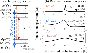
Figure 1: (a) Orbitals of parahelium (labeled by spectroscopic notation Levine (2000)), including three bound states and four autoionization resonances (above the ground-state energy of He⁺). Thick dashed arrows mark the probed transitions, while narrow arrows mark additional dipole-allowed transitions. (b–d) Autoionization spectrum [evaluated using Eq. (30) using data from Kaprálová-Žďánská and Šmydke (2013), summarized in Table S1 in the SI] near the three probed transitions from (a) and the associated $q$ factors [evaluated using Eq. (32)]. The $x$-axis is the difference between the frequency of the field and the probed atomic transition. [e.g., in (b), “zero frequency” implies that the probe is resonant with the $1s2p\leftrightarrow 2p^{2}$ transition.]

As an example for application of Eq. (32), we compute the absorption lineshape near AI states in parahelium (i.e., helium atoms in which the spins of the two electrons are in the singlet state). The energy levels and dipole-allowed transitions are shown in Fig. 1(a). The states are labeled according to the approximate Hartree–Fock orbitals. All states below the ionization threshold are bound, while all double-excitation states are metastable AI states. We use data from Refs. 14; 15 for the energy levels, lifetimes, and complex transition dipole moments (summarized in Table S1 in the SI). Figure 1(b–d) shows the ionization spectrum near three transitions in the XUV range, obtained by evaluating Eq. (30). The $x$-axis denotes the frequency offset between the field and the probed atomic transition. The plots demonstrate that our new formula for the Fano $q$ factor [Eq. (32)] predicts the asymmetry of the lines, while the width of the peak is set by the imaginary part of the metastable-state energy.

Next, we turn to study photoautoionization in laser-driven atoms and molecules. Specifically, we consider cases where a “pump laser” couples two (or more) AI states and a “probe laser” drives transitions from the ground to the AI states. A time-periodic probed system (denoted below by $H_{0}$) has Floquet solutions the form Dittrich et al. (1998):

$$\Psi_{\alpha,m}(x,t)=e^{-i\varepsilon_{\alpha,m}t/\hbar}\Phi_{\alpha,m}(x,t).$$ (33)

Here, $\Phi_{\alpha,m}$ and $\varepsilon_{\alpha,m}$ are the eigenvectors and eigenvalues of the Floquet Hamiltonian, $\mathcal{H}\equiv H_{0}-i\hbar\frac{\partial}{\partial t}$. The eigenenergies are periodic in the frequency of the probe, $\omega_{0}$ (i.e., $\varepsilon_{\alpha m}=\varepsilon_{\alpha,0}+m\hbar\omega_{0}$) and the eigenvectors obey $\Phi_{\alpha m}(t)=\Phi_{\alpha,0}(t)e^{i\omega_{0}mt}$. The quantum number $m$ is called the “Floquet channel.” In the SI, we use a generalized Fermi-Floquet golden rule Bilitewski and Cooper (2015) (which is valid for weak probe intensities) to derive a formula for the absorption spectrum of laser-driven systems. We obtain

$$S(\omega)=\frac{\left|\mathcal{E}\right|^{2}}{\hbar\pi}\mathrm{Im}\sum_{fm}\frac{(({\Phi_{i,0}^{L}}|x|{\Phi_{f,m}^{R}}))(({\Phi_{f,m}^{L}}|x|{\Phi_{i,0}^{R}}))}{\hbar\omega+m\hbar\omega_{0}-\varepsilon_{f,0}+\varepsilon_{i,0}}.$$ (34)

Here $|{\Phi_{i,0}})$ and $|{\Phi_{f,m}})$ are the initial (bound) and final (metastable) Floquet states while $\varepsilon_{i,0}$ and $\varepsilon_{f,0}$ are the corresponding quasienergies in the zeroth Floquet channel. We use double brackets to denote spatial and temporal integration: $(({\Phi}|{\Psi}))\equiv\frac{1}{T}\int_{0}^{T}dt^{\prime}\!\int_{-\infty}^{\infty}dx\,\,{\Phi(t^{\prime},x)}{\Psi(t^{\prime},x)}$. In order to evaluate Eq. (34), it is convenient to expand the Floquet states, $|{\Phi_{f,m}})$, in the basis of eigenvectors of the field-free Hamiltonian. In the SI, we review this standard procedure Chu and Reinhardt (1977); Chu (1985) and present an explicit expression for the spectrum in terms of field-free eigenstates [Eq. (C22)].

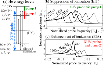
Figure 2: (a) Orbitals of parahelium (as in Fig. 1). Thick dashed (solid) arrows mark the probed (pumped) transitions, while narrow arrows mark other allowed transitions. (b) Pump 1 couples the probed AI state [$2s2p(^{1}P^{o})$] to the state $2p^{2}({{}^{1}}S^{e})$, whose lifetime is longer than $2s2p$. The pump produces a dip in the ionization spectrum when the probe is resonant with the probed transition, similar to EIT. (The $x$-axis is the probe’s detuning from resonance, as in Fig. 1.) Four pump amplitudes are shown: $\mathcal{E}/\mathcal{E}_{\mathrm{EP}}=1,2,6,10$, while the pump intensity is $\omega_{2}^{\mathrm{EP}}$ (see text). Helium parameters are summarized in Table S1. (c) Pump 2 couples the probed AI state to the state $2s^{2}(^{1}S^{e})$, whose lifetime is shorter than $2s2p$. The resulting ionization spectrum shows enhancement of ionization on resonance (similar to EIA).

Next, we apply Eq. (34) to compute the autoionization spectrum of laser-driven parahelium. As shown in Fig. 2(a), we consider an XUV probe, which drives the transition between the ground state [$1s^{2}\,(^{1}S)$] and the AI state $2s2p(^{1}P)$ and a strong NIR pump, which resonantly couples two AI states. We consider two cases: $(i)$ The pump couples $2s2p\,(^{1}P)$ and $2p^{2}\,(^{1}S)$ (green arrow) and $(ii)$ The pump couples $2s2p\,(^{1}P)$ and $2s^{2}\,(^{1}S)$ and (red arrow). The difference between the two cases is that in the former, the probe couples the ground state to the broader AI state (out of the two coupled AI states), while in the latter, the probe couples the ground state to the narrower AI state. It turns out that these two situations lead to drastically different ionization spectra. In the former case [shown in Fig. 2(b)], the effect of the pump is to suppress the ionization when the probe-photon energy is resonant with the atomic transition. The narrow dip in the autoionization spectrum is similar in spirit to the transparency window in EIT. As shown in the early work of Karapanagioti et al. (1995), the suppression occurs due to coherent trapping of the atomic population in the ground state. In contrast, in the latter case [shown in Fig. 2(c)], the ionization lineshape is Lorentzian for weak pump amplitudes [similar to electromagnetically induced absorption (EIA)]. As the pump exceeds a critical value (denoted by $\mathcal{E}_{0}=\mathcal{E}_{\mathrm{EP}}$), the peak splits into two non-overlapping dressed-state peaks. At the splitting point, the Hamiltonian has an EP, as discussed below. Panels (b–c) show the splitting of the ionization peaks upon increasing the pump amplitude beyond the critical point (we show four pump values $\mathcal{E}_{0}/\mathcal{E}_{\mathrm{EP}}=1,2,6,10$). Our ab-initio calculation takes into account all the dipole-allowed transitions in parahelium, although the atomic population predominantly occupies only three states in all cases under study.

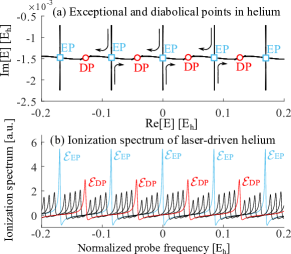
Figure 3: (a) Trajectories of eigenvalues of the Floquet Hamiltonian [Eqs. (C6-C7)] upon varying the pump amplitude across the EP value while fixing the pump frequency at $\omega_{2}^{\mathrm{EP}}$ (see text). Helium parameters are saummarized in Table S1. Pairs of eigenvalues merge at exceptional and diabolical points (EPs and DPs), marked by cyan triangles and red circles respectively. (b) Relative absorption as a function of probe detuning for six pump amplitudes: $\mathcal{E}_{0}/\mathcal{E}_{\mathrm{EP}}=1,11,22,33,44,55$. The peak absorption at EPs (cyan solid) is twice larger than DPs (red dashed). The $x$-axis denotes the frequency offset between the field and the probed atomic transition.

When the pump amplitude significantly exceeds $\mathcal{E}_{\mathrm{EP}}$ (at $\mathcal{E}\approx 70\mathcal{E}_{\mathrm{EP}}$), pairs of resonances merge again at ordinary degeneracies, called diabolical points (DPs). The trajectories of the complex eigenvalues of the Floquet Hamiltonian [see SI, Eqs. (C6-C7)] are shown in Fig. 3(a). Panel (b) shows the absorption spectrum at varying pump intensities for the case where the pump couples $2s^{2}\,(^{1}S)$ and $2s2p\,(^{1}P)$ [case $(ii)$ above]. The plot demonstrates that the peak of the ionization spectrum near the EPs is significantly larger than near the DPs (i.e., four-fold instead of two-fold), although the imaginary parts of the degenerate eigenvalues are approximately equal. This demonstrates the increased density of states at EPs (similar to the effect shown in spontaneous emission near EPs in Maxwell’s equations Pick et al. (2017)).

In order to see that the point at which the spectral peaks split is an EP, we introduce a simplified model, where we keep only three electronic states (i.e., we keep only the ground state and a pair of AI state) and employ the rotating wave approximation Scully and Zubairy (1997) (RWA) to eliminate rapidly rotating terms due to the pump and the probe. By using the RWA, a three-level system can be described by the stationary effective Hamiltonian Scully and Zubairy (1997); Kaprálová-Žďánská and Moiseyev (2014):

$$\mathbb{H}=\left(\begin{array}[]{c|cc}E_{g}+\hbar\omega_{1}&-\tfrac{\mu_{1}\mathcal{E}_{1}}{2}&0\\ \hline\cr-\tfrac{\mu_{1}\mathcal{E}_{1}}{2}&E_{1}-i\gamma_{1}&-\tfrac{\mu_{2}\mathcal{E}_{2}}{2}\\ 0&-\tfrac{\mu_{2}\mathcal{E}_{2}}{2}&E_{2}-i\gamma_{2}-\hbar\omega_{2}\end{array}\right)$$ (35)

Here, $E_{g}$ is the real ground-state energy, $E_{1,2}$ and $\gamma_{1,2}^{-1}$ are the excited-state energies and lifetimes and $\mu_{1,2}$ are the complex transition dipole moments of the allowed transitions. $\omega_{1,2}$ and $\mathcal{E}_{1,2}$ are the frequencies and amplitudes of the probe and pump fields respectively. The solid lines in Eq. (35) mark the excited-state Hamiltonian, $\mathbb{H}_{\mathrm{exc}}$ (introduced in the introduction), whose complex eigenvalues ($\varepsilon_{\pm}$) and eigenvectors ($\phi_{\pm}$) coalesce at an EP when the pump frequency and amplitude are Kaprálová-Žďánská and Moiseyev (2014)

$$\hbar\omega_{2}^{\mathrm{EP}}\equiv E_{1}-E_{2}+\frac{\gamma_{2}-\gamma_{1}}{2}\frac{\mathrm{Im}\,\mu_{2}}{\mathrm{Re}\,\mu_{2}}\quad,\quad\mathcal{E}_{2}^{\mathrm{EP}}\equiv\pm\frac{\gamma_{1}-\gamma_{2}}{2\,\mathrm{Re}\,\mu_{2}},$$ (36)

More details are given in the SI. When the pump intensity is fixed at $\omega_{2}^{\mathrm{EP}}$ and its amplitude exceeds the critical value of $\mathcal{E}_{2}^{\mathrm{EP}}$, the ionization peak splits into two since the dressed-state energies, $\mathrm{Re}[\varepsilon_{\pm}]$, become non degenerate. Similar to our conclusion here, it was also noted in Karapanagioti et al. (1995) that the splitting of spectral lines occurs when “the dipole coupling is strong enough to compete with the autoionizing width.” However, our non-Hermitian approach enables to identify this point as an EP and, therefore, opens the possibility of exploring EP-related effects near the splitting point.

To summarize, we presented an  ab-initio theory of resonant photoionization. Our derivation produced accurate formulas for the ionization spectrum, which are of current interest due to recent developments in experimental capabilities for probing and controlling ionization processes. By using NHQM, our theory avoids the need of computing the continuum states, which are required by the traditional Feshbach formalism. As an application of our theory, we derive a simple expression for the Fano asymmetry factor. Moreover, we study autoionization in laser driven systems and show that the splitting of spectral lines occurs at EPs. This work opens several directions for future study. For example, the non-trivial topological phase associated with the EP Mailybaev, Kirillov, and Seyranian (2005) can be used to transition between nearly degenerate states in a topologically protected manner Doppler et al. (2016), and may have practical applications for controlling the ionization spectrum. Another example for an EP-related effect is the enhanced density of states at the EP. Previous work on spontaneous emission Pick et al. (2017); Lin et al. (2016) shows that the emission rate can be significantly enhanced by placing the emitter near pumped resonators with EPs (i.e., using systems that have optical gain). Along similar lines, one can expect enhanced autoionization rates in systems with gain of atomic population in particular AI states. Such a situation can be engineered, for example, (e.g., in systems with cycling transitions Togan et al. (2011)). Finally, the present work treated broadening of absorption lines due to autoionization, but can be extended to include other line-broadening mechanism (such as vibrational and Doppler broadening) by combining NHQM with a Lindbladian formulation.

Supplementary Information

I Green’s function Near EPs

Near an EP, the non-Hermitian normal-mode expansion formula for the Green’s function [Eq. (5)] breaks down. In this appendix, we review the derivation of the modified expansion formula which is valid at the EP, following Pick et al. (2017). Consider the parameter-dependent Hamiltonian:

$$H(\xi)=H_{0}+\xi V$$ (A1)

where $H_{0}$ is defective (i.e., the point $\xi=0$ is an EP in parameter space). At the EP, the set of eigenvectors is no longer a complete basis of the Hilbert space. To remedy this problem, we introduce additional Jordan vectors. At a second-order EP, the Jordan vector $|{j_{\mathrm{EP}}})$ is defined via the chain relations

$$H_{0}|{\phi_{\mathrm{EP}}})=\varepsilon_{\mathrm{EP}}|{\phi_{\mathrm{EP}}}),$$

$$H_{0}|{j_{\mathrm{EP}}})=\varepsilon_{\mathrm{EP}}|{j_{\mathrm{EP}}})+|{\phi_{\mathrm{EP}}}).$$ (A2)

where $\varepsilon_{\mathrm{EP}}$ and $\phi_{\mathrm{EP}}$ are the degenerate eigenvalue and eigenvector and the self-orthogonality condition [$({\phi_{\mathrm{EP}}}|{\phi_{\mathrm{EP}}})=0$] is automatically satisfied. Following Seyranian and Mailybaev (2003), we choose the normalization conditions $({\phi_{\mathrm{EP}}}|{j_{\mathrm{EP}}})=\varepsilon_{\mathrm{EP}}^{-1}$ and $({j_{\mathrm{EP}}}|{j_{\mathrm{EP}}})=0$. Near the EP at $\xi=0$, the Hamiltonian $H(\xi)$ has a pair of nearly degenerate eigenenergies and nearly parallel eigenvectors. They can be approximated by a Puiseux series, which contains fractional powers in the small parameter $\xi$ Seyranian and Mailybaev (2003):

$$\varepsilon_{{\pm}}=\varepsilon_{\mathrm{EP}}+\sqrt{\xi}\,\mathcal{V}+\mathcal{O}(\xi)$$

$$|{\phi_{\pm}})=|{\phi_{\mathrm{EP}}})+\sqrt{\xi}\,\mathcal{V}|{j_{\mathrm{EP}}})+\mathcal{O}(\xi)$$ (A3)

where

$$\mathcal{V}=\sqrt{\frac{({j_{\mathrm{EP}}}|{V}|{\phi_{\mathrm{EP}}})}{({j_{\mathrm{EP}}}|{\phi_{\mathrm{EP}}})}}.$$ (A4)

Now, let us return to the modal expansion formula of $G$ [Eq. (5)], which is valid for $\xi\neq 0$. Near the EP, the expansion is dominated by the two terms of the coalescing resonances. Keeping just these two terms in the sum, we can write

$$G(\varepsilon)=\frac{1}{\varepsilon-\varepsilon_{+}}\frac{|{\phi_{+}})({\phi_{+}}|}{({\phi_{+}}|{\phi_{+}})}+\frac{1}{\varepsilon-\varepsilon_{-}}\frac{|{\phi_{-}})({\phi_{-}}|}{(\phi_{-}|\phi_{-})}$$ (A5)

Next, we substitute the approximate expressions for $|{\phi_{\pm}})$ and $\varepsilon_{\pm}$ [Eq. (A3)] into Eq. (A5) and, by carefully taking the limit of $\xi\rightarrow 0$, we obtain Pick et al. (2017)

$$G(\varepsilon)=\frac{1}{(\varepsilon-\varepsilon_{\mathrm{EP}})^{2}}\frac{|{\phi_{\mathrm{EP}}})({\phi_{\mathrm{EP}}}|}{(\phi_{\mathrm{EP}}|j_{\mathrm{EP}})}+$$

$$\frac{1}{\varepsilon-\varepsilon_{\mathrm{EP}}}\left(\frac{|{\phi_{\mathrm{EP}}})({j_{\mathrm{EP}}}|}{(\phi_{\mathrm{EP}}|j_{\mathrm{EP}})}+\frac{|{j_{\mathrm{EP}}})({\phi_{\mathrm{EP}}}|}{(\phi_{\mathrm{EP}}|j_{\mathrm{EP}})}\right)$$ (A6)

The double pole at $\varepsilon_{\mathrm{EP}}$ dominates the absorption spectrum near the EP.

II Non-Hermitian Fano factor

In this appendix, we derive Eq. (8) from the main text. The formula is obtained by comparing the ratio of the symmetric and antisymmetric parts of our new spectral formula [Eq. (6)] and the Fano lineshape near a single resonance [Eq. (7)]. First, let us introduce the dimensionless detuning parameter $x=\frac{\omega-\Omega}{\gamma/2}$ and rewrite Eq. (7) as

$$S_{F}=1+\frac{2xq}{x^{2}+1}+\frac{q^{2}-1}{x^{2}+1}$$ (B1)

Next, let us define the symmetric and antisymmetric parts of our absorption formula as

$$S_{\mathrm{symm}}=\frac{|\mathcal{E}|^{2}}{\hbar\pi}\frac{\mathrm{Re}\,\mu_{if}^{2}\mathrm{Im}\,\varepsilon_{f}}{(\omega-\mathrm{Re}\,\varepsilon_{f})^{2}+(\mathrm{Im}\,\varepsilon_{f})^{2}},$$

$$S_{\mathrm{asymm}}=\frac{|\mathcal{E}|^{2}}{\hbar\pi}\frac{\mathrm{Im}\,\mu_{if}^{2}(\mathrm{Re}\,\varepsilon_{f}-\omega)}{(\omega-\mathrm{Re}\,\varepsilon_{f})^{2}+(\mathrm{Im}\varepsilon_{f})^{2}},$$ (B2)

where introduced the shorthand notation $\mu_{if}^{2}=({\phi_{i}^{L}}|x|{\phi_{f}^{R}})({\phi_{f}^{L}}|x|{\phi_{i}^{R}})$. By comparing Eq. (B1) and Eq. (B2) we find that

$$\frac{2q}{q^{2}-1}=\frac{\mathrm{Im}\,\mu_{if}^{2}}{\mathrm{Re}\,\mu_{if}^{2}}.$$ (B3)

The solution of Eq. (B3) yields the Fano asymmetry factor [Eq. (8)]. The sign of $q$ is determined by the sign of $\mathrm{Im}\,\mu_{ij}^{2}$. When $q>0$, the absorption is stronger at frequencies higher than the resonance frequency and weaker below the resonance. When $q<0$, the contrary is true.

III Absorption in laser-driven systems

III.1 The Floquet Hamiltonian

In this section, we explain how to construct the Floquet Hamiltonian and find its eigenvalues and eigenvectors, which appear in Eq. (10) in the main text. We wish to solve the Floquet eigenvalue problem

$$\mathcal{H}\Phi_{\alpha}=\varepsilon_{\alpha}\Phi_{\alpha},$$ (C1)

where

$$\mathcal{H}\equiv H_{0}+\mathcal{E}x\cos{\omega_{0}t}-i\hbar\partial_{t}.$$ (C2)

In order to solve Eq. (C1) numerically, we introduce $M$ temporal Fourier basis states, $f_{m}(t)=e^{i\omega mt}$, and $N$ spatial field-free states, $\phi^{\mathrm{FF}}_{\mu}(x)$. Invoking the completeness relation,

$$\mathbb{1}=\sum_{m=1}^{M}|{f_{m}(t)})({f_{m}(t)}|\otimes\sum_{\mu=1}^{N}|{\phi_{\mu}^{\mathrm{R,FF}}(x)})({\phi_{\mu}^{\mathrm{L,FF}}(x)}|,$$ (C3)

we can rewrite Eq. (C1) in matrix form:

$$\sum_{m,\nu}({n,\nu}|\mathcal{H}|{m,\mu})({m,\mu}|{\Phi_{\alpha}})=\varepsilon_{\alpha}({n,\nu}|{\Phi_{\alpha}})$$ (C4)

or in shorthand notation:

$$\overline{\overline{\mathcal{H}}}\,\vec{\Phi}_{\alpha}=\varepsilon_{\alpha}\vec{\Phi}_{\alpha},$$ (C5)

where $\overline{\overline{\mathcal{H}}}$ is block diagonal, with block size $M\times M$. The diagonal blocks are associated with the first and last terms in Eq. (C2)

$$\overline{\overline{\mathcal{H}}}_{\mu n,\nu n}=(\varepsilon_{\mu}^{\mathrm{FF}}+n\hbar\omega_{0})\delta_{\mu,\nu}$$ (C6)

and the off-diagonal elements come from the second term:

$$\overline{\overline{\mathcal{H}}}_{\mu n,\nu n\pm 1}=\tfrac{\mathcal{E}}{2}({\phi^{\mathrm{L,FF}}_{\mu}}|x|{\phi^{\mathrm{R,FF}}_{\nu}})$$ (C7)

III.2 Fermi-Floquet absorption formula

In this appendix, we complete the derivation of Eq. (10) from the main text. Our derivation is inspired by Ref. Bilitewski and Cooper (2015), which analyzes scattering from a time-periodic potential. Consider an atom or molecule, which interacts with a laser at frequency $\omega_{0}$. The system is described by the Hamiltonian $H_{0}$, whose eigenstates are Floquet states, as explained in the main text. The propagator of $H_{0}$ is defined via

$$i\hbar\partial_{t}U_{0}(t_{0},t)=H_{0}(t)U_{0}(t_{0},t).$$ (C8)

We also introduce a weak laser, hereafter called “the probe,” with frequency $\omega$. The total Hamiltonian is

$$H=H_{0}+V,$$ (C9)

where the interaction term is $V=\mathcal{E}xe^{i\omega t}$. In order to derive Fermi-Floquet golden rule, we move to the interaction picture, where states and operators are defined as

$$|{\Psi^{I}(t)})=U_{0}(t,t_{0})|{\Psi(t)})$$

$$\mathcal{O}^{I}(t)=U_{0}(t,t_{0})\mathcal{O}U_{0}(t_{0},t).$$ (C10)

Note that the total propagator, defined as

$$i\hbar\partial_{t}U(t_{0},t)=H(t)U(t_{0},t),$$ (C11)

can be written as a product of the unperturbed and interaction-picture propagators:

$$U(t_{0},t)=U_{0}(t_{0},t)U^{I}(t_{0},t).$$ (C12)

The last statement can be verified by substituting Eq. (C12) into Eq. (C11), applying the chain rule to compute $\partial_{t}U(t,t_{0})$, and using Eq. (C8) and $V^{I}=U_{0}(t,t_{0})VU_{0}(t_{0},t)$.

Next, we compute the transition amplitude between Floquet states $|{\Psi_{f}(t)})$ and $|{\Psi_{i}(t)})$, where $i$ and $f$ are super-indexes which denote the field-free state and the channel. The transition amplitude is

$$A(i\rightarrow f,t)=({\Psi_{f}(t)}|U(0,t)|{\Psi_{i}(0)})=$$

$$({\Psi_{f}(t)}|U_{0}(0,t)U^{I}(0,t)|{\Psi_{i}(0)})=$$

$$({\Psi_{f}(0)}|U^{I}(0,t)|{\Psi_{i}(0)})$$ (C13)

We use a Dyson series to express the interaction-picture propagator, $U^{I}$,in terms of $V^{I}$. Keeping terms up to the first order in $V^{I}$, one obtains:

$$U^{I}(t_{0},t)=\mathbb{1}-\frac{i}{\hbar}\int_{t_{0}}^{t}dt^{\prime}V^{I}(t^{\prime})+\mathcal{O}(V^{2}).$$ (C14)

Substituting Eq. (C14) into Eq. (C13), one obtains

$${A(i\rightarrow f,t)=\frac{-i}{\hbar}\int_{0}^{t}dt^{\prime}({\Psi_{f}(0)}|V^{I}(0,t^{\prime})|{\Psi_{i}(0)})=}$$

$${\frac{-i}{\hbar}\int_{0}^{t}dt^{\prime}({\Psi_{f}(0)}|U_{0}(t^{\prime},0)VU_{0}(0,t^{\prime})|{\Psi_{i}(0)})=}$$

$${\frac{-i}{\hbar}\int_{0}^{t}dt^{\prime}e^{-i(\varepsilon_{i}-\varepsilon_{f})t^{\prime}/\hbar}({\Phi_{f}(t^{\prime})}|V|{\Phi_{i}(t^{\prime})}).}$$ (C15)

Since the Floquet states $\Phi_{\alpha}(x,t)$ are periodic in time, one can decompose them into Fourier components

$$\Phi_{\alpha}(x,t)=\sum_{n}e^{i\omega_{0}nt}\tilde{\phi}_{\alpha,n}(x)$$ (C16)

where the Fourier components of the wavefunction are $\tilde{\phi}_{\alpha,n}(x)\equiv\frac{1}{\sqrt{2\pi}}\int_{-\infty}^{\infty}dt\,\Phi_{\alpha}(x,t)e^{-i\omega_{0}mt}$. Using this expansion, the transition amplitude becomes

$${A(i\rightarrow f,t)=}$$

$${\sum_{mn}\frac{-i\mathcal{E}}{\hbar}\int_{0}^{t}dt^{\prime}e^{-i(\varepsilon_{i}-\varepsilon_{f}-(n-m)\hbar\omega_{0}-\hbar\omega)t^{\prime}/\hbar}({\tilde{\phi}_{f,n}}|x|{\tilde{\phi}_{i,m}})=}$$

$${\mathcal{E}\sum_{mn}\frac{e^{-i(\varepsilon_{i}-\varepsilon_{f}-m\hbar\omega_{0}-\hbar\omega)t/\hbar}-1}{\varepsilon_{i}-\varepsilon_{f}-m\hbar\omega_{0}-\hbar\omega}({\tilde{\phi}_{f,m+n}}|x|{\tilde{\phi}_{i,m}}).}$$ (C17)

The absorption spectrum can be found by taking the time average of the transition probability:

$${S(\omega)\equiv\frac{1}{T}\int_{0}^{T}\!dt\,\frac{d}{dt}|A_{if}|^{2}=2\mathrm{Re}\left[\frac{1}{T}\int_{0}^{T}\!dt\,A^{*}\frac{dA}{dt}\right],}$$ (C18)

where $T$ is a large integer multiple of the oscillation period $\frac{2\pi}{\omega_{0}}$. Substituting Eq. (C17) into Eq. (C18) and neglecting rapidly oscillating terms, we obtain

$$\frac{1}{T}\int_{0}^{T}dt\,A^{*}\frac{dA}{dt}=\frac{-i|\mathcal{E}|^{2}}{\hbar}\sum_{mn\ell}\frac{({\tilde{\phi}_{f,m+n}}|x|{\tilde{\phi}_{i,m}})({\tilde{\phi}_{i,m}}|x|{\tilde{\phi}_{f,m+\ell}})}{(\varepsilon_{i}-\varepsilon_{f}-m\hbar\omega_{0}-\hbar\omega)}$$ (C19)

Finally, we take the real part of Eq. (C19) and arrive at

$${S(\omega)=\frac{|\mathcal{E}|^{2}}{\hbar}\mathrm{Im}\left[\sum_{mn\ell}\frac{({\tilde{\phi}^{L}_{f,m+n}}|x|{\tilde{\phi}^{R}_{i,m}})({\tilde{\phi}^{L}_{i,\ell}}|x|{\tilde{\phi}^{R}_{f,\ell+m}})}{\varepsilon_{i}-\varepsilon_{f}-m\hbar\omega_{0}-\hbar\omega}\right]}$$ (C20)

The last formula can be rewritten compactly as Eq. (10) in the main text.

III.3 Autoionization spectral formula in the field-free basis

In order to evaluate our new formula for the absorption spectrum [Eq. (C20) or equivalently Eq. (10) from the main text], we need to know the Fourier transforms of Floquet states. However, standard quantum chemistry methods solve the field-free problem, and we would like to use the field-free basis states and avoid the formidable task of solving the Floquet eigenvalue problem for a multielectron atom or molecule. To this end, we expand the Fourier transforms of the Floquet states in the basis of field-free states.

$$|{\tilde{\phi}_{\alpha,n}})=\sum_{\mu}({\phi^{\mathrm{FF}}_{\mu}}|{\tilde{\phi}_{\alpha,n}})|{\phi^{\mathrm{FF}}_{\mu}})$$ (C21)

Substituting Eq. (C21) into Eq. (C20), we obtain

$${S(\omega)=\frac{|\mathcal{E}|^{2}}{\hbar}\mathrm{Im}\left[\sum_{\begin{subarray}{c}mn\ell\\ \mu\nu\sigma\tau\end{subarray}}({\tilde{\phi}^{L}_{i,\ell}}|{\phi^{\mathrm{FF}}_{\tau}})({\phi^{\mathrm{FF}}_{\tau}}|x|{\phi^{\mathrm{FF}}_{\sigma}})\right.}$$

$${\left.\frac{({\phi^{\mathrm{FF}}_{\sigma}}|{\tilde{\phi}^{R}_{f,\ell+m}})({\tilde{\phi}^{L}_{f,n+m}}|{\phi^{\mathrm{FF}}_{\mu}})}{\varepsilon_{i}-\varepsilon_{f}-m\hbar\omega_{0}-\hbar\omega}({\phi^{\mathrm{FF}}_{\mu}}|x|{\phi^{\mathrm{FF}}_{\nu}})({\phi^{\mathrm{FF}}_{\nu}}|{\tilde{\phi}^{R}_{i,n}})\right]}$$ (C22)

The transition dipole moments between field-free states, $({\phi^{\mathrm{FF}}_{\tau}}|x|{\phi^{\mathrm{FF}}_{\sigma}})$, are obtained directly from available quantum chemistry codes. By construction, the expansion coefficients, $({\phi^{\mathrm{FF}}_{\mu}}|{\tilde{\phi}^{R}_{\alpha,n}})$, are the components of the eigenvectors of the Floquet matrix:

$$({\phi^{\mathrm{L,FF}}_{\mu}}|{\tilde{\phi}^{R}_{\alpha,m}})=({m,\mu}|{\Phi^{R}_{\alpha}}).$$ (C23)

The eigenvectors of the Floquet Hamiltonian, $({m,\mu}|{\Phi^{R}_{\alpha}})$, are defined in Eq. (C4).

III.4 EPs in the Floquet Hamiltonian

To get an initial guess for the location of the EP, it is convenient project the full Hamiltonian onto the field-free excited states $\psi_{2}$ and $\psi_{3}$ and use the rotating wave approximation, which gives the $2\times 2$ Hamiltonian

$$H_{\mathrm{exc}}=\left(\begin{array}[]{cc}E_{2}&-\tfrac{\mu_{23}\mathcal{E}}{2}\\ -\tfrac{\mu_{32}\mathcal{E}}{2}&E_{3}-\hbar\omega_{0}\end{array}\right).$$ (C24)

Subtracting $E_{2}$ from the diagonal and introducing the definitions $\delta\equiv\mathrm{Re}[E_{3}-E_{2}-\hbar\omega_{0}]$ and $\Gamma\equiv-2\mathrm{Im}[E_{3}-E_{2}]$, we obtain

$$H_{\mathrm{exc}}=\left({\begin{array}[]{cc}0&-\tfrac{\mu_{23}\mathcal{E}}{2}\\ -\tfrac{\mu_{23}\mathcal{E}}{2}&\delta-i\tfrac{\Gamma}{2}\end{array}}\right).$$ (C25)

The characteristic polynomial of $H_{\mathrm{exc}}$ is

$$f(x)=x^{2}-x(\delta-i\tfrac{\Gamma}{2})-\tfrac{(\mu_{23}\mathcal{E})^{2}}{4},$$ (C26)

and EPs occur when the discriminant of the polynomial vanishes:

$$\Delta^{2}\equiv(\tfrac{\delta}{2}-i\tfrac{\Gamma}{4})^{2}+\tfrac{(\mu_{23}\mathcal{E})^{2}}{4}=0$$ (C27)

Solving for $\mathcal{E}$ and $\delta$, we obtain the critical values Kaprálová-Žďánská and Moiseyev (2014):

$$\delta_{\mathrm{EP}}=\frac{\Gamma}{2}\frac{\mathrm{Im}\,\mu_{23}}{\mathrm{Re}\,\mu_{23}}\hskip 72.26999pt\mathcal{E}_{\mathrm{EP}}=\pm\frac{\Gamma}{2\,\mathrm{Re}\,\mu_{23}}$$ (C28)

In the numerical calculation, we found EPs in the large ($MN\times MN$) Floquet Hamiltonian, including four field-free basis states and five Floquet bands, but found that the EP is obtained near the EP of the approximate $2\times 2$ model. Specifically, we find an EP of the full Floquet Hamiltonian at $\delta\approx 1.001645\,\delta_{\mathrm{EP}}$ and $\mathcal{E}\approx 0.99420\,\mathcal{E}_{\mathrm{EP}}$.

IV Electronic-structure of Helium

Table S1 summarizes the complex energies and transition dipole moments for lowest-energy single- and double-excitation states in helium. The numerical values were obtained by Kaprálová-Žďánská et. al. Kaprálová-Žďánská, Šmydke, and Civiš (2013), and are used in all the calculations in the main text. For copmarison, we show additional ab-initio results from Gilary, Kaprálová-Žd’ánská, and Moiseyev (2006), which demonstrate good agreement between different methods for the set of energy levels that we consider.

Table S1: Complex energies (top) and transition dipole moments (bottom) for helium, obtained from ab-initio calculations in Refs. 14; 68.

		Re[E] Gilary, Kaprálová-Žd’ánská, and Moiseyev (2006)	Re[E] Kaprálová-Žďánská, Šmydke, and Civiš (2013)	Im[E] Gilary, Kaprálová-Žd’ánská, and Moiseyev (2006)	Im[E] Kaprálová-Žďánská, Šmydke, and Civiš (2013)
1	$1s^{2}$	-2.90372	-2.9035	0	0
2	1s2s	-2.14597	-2.1460	0	0
3	1s2p	-2.12384	-2.1238	0	0
4	$2s^{2}$	-0.777868	-0.7779	0.002271	-0.0023
5	$2p^{2}$	-0.710500	-0.7018	0.001181	-0.0012
6	2s2p	-0.693135	-0.6930	0.0006865	-0.0007
7	$2p^{2}$	-0.621926	-0.6216	0.000108	-0.0001

	$\mu_{R}$ Kaprálová-Žďánská, Šmydke, and Civiš (2013)	$\mu_{I}$ Kaprálová-Žďánská, Šmydke, and Civiš (2013)	$\lambda$ [nm]
$1\leftrightarrow 3$	0.4207	0.00000189	58.44 (UV)
$1\leftrightarrow 6$	0.03599	0.01299	20.61(UV)
$2\leftrightarrow 3$	2.9167	0.000004652	2058.47 (IR)
$2\leftrightarrow 6$	0.3130	-0.003598	31.36 (UV)
$3\leftrightarrow 4$	-0.1231	-0.002554	33.85 (UV)
$3\leftrightarrow 5$	0.3288	0.000193	32.04 (UV)
$3\leftrightarrow 7$	-0.1925	0.0003475	30.33 (UV)
$4\leftrightarrow 6$	1.5227	-0.00973	536.95 (visible)
$5\leftrightarrow 6$	1.70545	-0.003767	5160.2 (IR)
$6\leftrightarrow 7$	-2.1614	-0.001007	638.15 (visible)

References

- Krausz and Ivanov (2009) F. Krausz and M. Ivanov, “Attosecond physics,” Rev. Mod. Phys. 81, 163 (2009).
- Itatani et al. (2004) J. Itatani, J. Levesque, D. Zeidler, H. Niikura, H. Pépin, J. C. Kieffer, P. B. Corkum, and D. M. Villeneuve, “Tomographic imaging of molecular orbitals,” Nature 432, 867 (2004).
- Paul et al. (2001) P. M. Paul, E. S. Toma, P. Breger, G. Mullot, F. Augé, P. Balcou, H. G. Muller, and P. Agostini, “Observation of a train of attosecond pulses from high harmonic generation,” Science 292, 1689–1692 (2001).
- Klünder et al. (2011) K. Klünder, J. M. Dahlström, M. Gisselbrecht, T. Fordell, M. Swoboda, D. Guenot, P. Johnsson, J. Caillat, J. Mauritsson, A. Maquet, J. Caillat, J. Mauritsson, A. Maquet, , and R. Taïeb, “Probing single-photon ionization on the attosecond time scale,” Phys. Rev. Lett. 106, 143002 (2011).
- Azoury et al. (2017) D. Azoury, M. Krüger, G. Orenstein, H. R. Larsson, S. Bauch, B. D. Bruner, and N. Dudovich, “Self-probing spectroscopy of XUV photo-ionization dynamics in atoms subjected to a strong-field environment,” Nature Comm. 8, 1453 (2017).
- Feshbach (1962) H. Feshbach, “A unified theory of nuclear reactions. II,” Ann. Phys. 19, 287–313 (1962).
- Friedrich and Wintgen (1985) H. Friedrich and D. Wintgen, “Interfering resonances and bound states in the continuum,” Phys. Rev. A 32, 3231 (1985).
- Averbukh and Cederbaum (2005) V. Averbukh and L. S. Cederbaum, “Ab-initio calculation of interatomic decay rates by a combination of the Fano ansatz, Green’s-function methods, and the stieltjes imaging technique,” J. Chem. Phys. 123, 204107 (2005).
- Goetz et al. (2017) R. E. Goetz, T. A. Isaev, B. Nikoobakht, R. Berger, and C. P. Koch, “Theoretical description of circular dichroism in photoelectron angular distributions of randomly oriented chiral molecules after multi-photon photoionization,” J. Chem. Phys. 146, 024306 (2017).
- Moiseyev (2011) N. Moiseyev, Non-Hermitian Quantum Mechanics (Cambridge University Press, 2011).
- Fano (1961) U. Fano, “Effects of configuration interaction on intensities and phase shifts,” Phys. Rev. 124, 1866 (1961).
- Autler and Townes (1955) S. H. Autler and C. H. Townes, “Stark effect in rapidly varying fields,” Phys. Rev. 100, 703 (1955).
- Kato (2013) T. Kato, Perturbation Theory for Linear Operators, Vol. 132 (Springer Science & Business Media, 2013).