The Alpha-Heston Stochastic Volatility Model

Abstract

We introduce an affine extension of the Heston model where the instantaneous variance process contains a jump part driven by $\alpha$-stable processes with $\alpha\in(1,2]$. In this framework, we examine the implied volatility and its asymptotic behaviors for both asset and variance options. Furthermore, we examine the jump clustering phenomenon observed on the variance market and provide a jump cluster decomposition which allows to analyse the cluster processes.

MSC: 91G99, 60G51, 60J85

Key words: Stochastic volatility and variance, affine models, CBI processes, implied volatility surface, jump clustering.

1 Introduction

The stochastic volatility models have been widely studied in literature and one important approach consists of the Heston model [27] and its extensions. In the standard Heston model, the instantaneous variance is a square-root mean-reverting CIR (Cox-Ingersoll-Ross [10]) process. On one hand, compared to the Black-Scholes framework, Heston model has the advantage to reproduce some stylized facts in equity and foreign exchange option markets. The model provides analytical tractability of pricing formulas which allows for efficient calibrations. On the other hand, the limitation of Heston model has also been carefully examined. For example, it is unable to produce extreme paths of volatility during the crisis periods, even with very high volatility of volatility (vol-vol) parameter. In addition, the Feller condition, which is assumed in Heston model to ensure that the volatility remains strictly positive, is often violated in practice, see e.g. Da Fonseca and Grasselli [11].

To provide more consistent results with empirical studies, a natural extension is to consider jumps in the stochastic volatility models. In the Heston framework, Bates [5] adds jumps in the dynamics of the asset, while Sepp [42] includes jumps in both asset returns and the variance, both papers using Poisson processes. In Barndorff-Nielsen and Shephard [4], the volatility process is the superposition of a family of positive non-Gaussian Ornstein-Uhlenbeck processes. Nicolato et al. [40] study the case where a jump term is added to the instantaneous variance process which depends on an increasing and driftless Lévy process, and they analyze the impact of jump diffusions on the realized variance smile and the implied volatility of VIX options. More generally, Duffie et al. [13] [14] propose the affine jump-diffusion framework for the asset and stochastic variance processes. There are also other extensions of Heston model. Grasselli [23] combines standard Heston model with the so-called $3/2$ model where the volatility is the inverse of the Heston one. Kallsen et al [32] consider the case where stock evolution includes a time-change Lévy process. In the framework of rough volatility models (see for example El Euch et al. [17] and Gatheral et al. [21]), El Euch and Rosenbaum [16] propose the rough Heston model where the Brownian term is replaced by a fractional Brownian motion and they provide the characteristic function by using the fractional Riccati equation.

In this paper, we introduce an extension of Heston model, called the $\alpha$-Heston model, by adding a self-exciting jump structure in the instantaneous variance. On financial markets, the CBOE’s Volatility Index (VIX) has been introduced as a measure of market volatility of S&P500 index. Starting from 2004, this index is exchanged via the VIX futures, and its derivatives have been developed quickly in the last decade. Figure 1 presents the daily closure values of VIX index from January 2004 to July 2017.

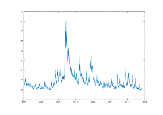
Figure 1: The CBOE’s VIX value from January 2004 to July 2017.

The historical data shows clearly that the VIX can have very large variations and jumps, particularly during the periods of crisis and partially due to the lack of “storage”. Moreover the jumps occur frequently in clusters. We note several significant jump clusters, the first one associated to the subprime crisis during 2008-2010, the second associated to the sovereign crisis of Greece during 2010-2012, and the last one to the Brexit event around 2016-2017. Between the jump clusters, the VIX values drop to relatively low levels during normal periods. One way to model the cluster effect in finance is to adopt the Hawkes processes [26] where it needs to specify the jump process together with its intensity. So the inconvenience is that the dimension of the concerned stochastic processes is increased. For the volatility data, El Euch et al. [17] emphasize that the market is highly endogenous and justify the use of nearly unstable Hawkes processes in their framework. Furthermore, Jaisson and Rosenbaum [29] prove that nearly unstable Hawkes processes converge to a CIR process after suitable rescaling. Therefore it is natural to reconcile the Heston framework with a suitable jump structure in order to describe the jump clusters.

Compared to the standard Heston model, the $\alpha$-Heston model includes an $\alpha$-root term and a compensated $\alpha$-stable Lévy process in the stochastic differential equations (SDE) of the instantaneous variance process $V=(V_{t},t\geq 0)$. The number of extra parameters is sparing and the only main parameter $\alpha$ determines the jump behavior. This model allows to describe the cluster effect in a parsimonious and coherent way. We adopt a related approach of continuous-state branching processes with immigration (CBI processes). With the general integral characterization for SDE in Dawson and Li [12], $V$ can be seen as a marked Hawkes process with infinite activity influenced by a Brownian noise (see Jiao et al. [30]), which is suitable to model the self-exciting jump property. In this model, the $\alpha$-stable jump process is leptokurtotic and heavy-tailed. The parameter $\alpha$ corresponds to the Blumenthal-Getoor index. Hence it’s able to seize both large and small fluctuations and even extreme high peaks during the crisis period. In addition, the law of jumps follows the Pareto distribution. Empirical regularities in economics and finance often suggest the form of Pareto law: Liu et al. [37] found that the realized volatility matches with a power law tail; more recently, Avellaneda and Papanicolaou [2] showed that the right-tail distribution of VIX time series can be fitted to a Pareto law. We note that the same Feller condition applies as in the standard Heston case and this condition is more easily respected by the $\alpha$-Heston model since the behavior of small jumps with infinite activity is similar to a Brownian motion so that the jump part allows to reduce the vol-vol parameter.

Thanks to the link between CBI and affine processes established by Filipović [19], our model belongs to the class of affine jump-diffusion models in Duffie et al. [13], [14] and the general result on the characteristic functions holds for the $\alpha$-Heston jump structure. However, the associated generalized Riccati operator is not analytic, which breaks down certain arguments borrowed from complex analysis. One important point is that although theoretical results on generalized Riccati operators are established for general affine models, in many explicit examples, the generalized Riccati equation which is associated to the state-dependent variable of $V$ is quadratic. The $\alpha$-Heston model allows to add more flexibility to the cumulant generator function since its generalized Riccati operator contains a supplementary $\alpha$-power term. We examine the moment explosion behaviors of both asset and variance processes following Keller-Ressel [33]. We are also interested in the implied volatility surface and its asymptotic behaviors based on the model-free result of Lee [34]. For the asset options, we show that the wing behaviors of the volatility smile at extreme strikes are the sharpest. For the variance options, we first estimate the asymptotic property of tail probability of the variance process.

One of the most interesting features of the $\alpha$-Heston model is that by using the CBI characteristics as in Li and Ma [36], we can thoroughly analyse the jump cluster effect. Inspired by Duquesne and Labbe [15], we provide a decomposition formula for the variance process $V$ which contains a fundamental part together with a sequence of jump cluster processes. This decomposition implies a branching structure in the sense that each cluster process is induced by a “mother jump” which is followed by “child jumps”. The mother jump represents a triggering shock on the market and is driven by exogenous news in general whereas the child jumps may reflect certain contagious effect. We then study relevant properties such as the duration of one cluster and the number of clusters occurred in a given period. We are particularly interested in the role played by the main parameter $\alpha$.

The rest of the paper is organized as follows. We present the model framework in Section 2. Section 3 is devoted to the affine characterization of the model and related properties. In Section 4, we study the asymptotic implied volatility behavior of asset and variance options. Section 5 deals with the analysis of jump clusters. We conclude the paper by providing the proofs in Appendix.

2 Model framework

Let us fix a probability space $(\Omega,\mathcal{A},\mathbb{Q})$ equipped with a filtration $\mathbb{F}=(\mathcal{F}_{t})_{t\geq 0}$ which satisfies the usual conditions. We first present a family of stochastic volatility models by using a general integral representation of SDEs with random fields. Consider the asset price process $S=(S_{t},t\geq 0)$ given by

$$\frac{dS_{t}}{S_{t}}=rdt+\int_{0}^{V_{t}}B(dt,du),\quad S_{0}>0$$ (1)

where $r\in\mathbb{R}_{+}$ is the constant interest rate, $B(ds,du)$ is a white noise on $\mathbb{R}_{+}^{2}$ with intensity $dsdu$, and the process $V=(V_{t},t\geq 0)$ is given by

$$V_{t}=V_{0}+\int_{0}^{t}a(b-V_{s})ds+\sigma\int_{0}^{t}\int_{0}^{V_{s}}W(ds,du)+\sigma_{N}\int_{0}^{t}\int_{0}^{V_{s-}}\int_{\mathbb{R}^{+}}\zeta\widetilde{N}(ds,du,d\zeta)$$ (2)

where $a,b,\sigma,\sigma_{N}\in\mathbb{R}_{+}$, $W(ds,du)$ is a white noise on $\mathbb{R}_{+}^{2}$ correlated to $B(ds,du)$ such that $B(ds,du)=\rho W(ds,du)+\sqrt{1-\rho^{2}}\overline{W}(ds,du)$ with $\overline{W}(ds,du)$ being an independent white noise and $\rho\in(-1,1)$, $\widetilde{N}(ds,du,d\zeta)$ is an independent compensated Poisson random measure on $\mathbb{R}_{+}^{3}$ with intensity $dsdu\nu(d\zeta)$ with $\nu(d\zeta)$ being a Lévy measure on $\mathbb{R}_{+}$ and satisfying $\int_{0}^{\infty}(\zeta\wedge\zeta^{2})\nu(d\zeta)<\infty$. The measure $\mathbb{Q}$ stands for the risk-neutral probability measure. We shall discuss in more detail the change of probability in Section 3.1.

The variance process $V$ defined above is a CBI process (c.f. Dawson and Li [12, Theorem 3.1]) with the branching mechanism given by

$$\Psi(q)=aq+\frac{1}{2}\sigma^{2}q^{2}+\int_{0}^{\infty}(e^{-q\sigma_{N}\zeta}-1+q\sigma_{N}\zeta){\nu}(d\zeta)$$ (3)

and the immigration rate $\Phi(q)=abq$. The existence and uniqueness of a strong solution of (2) is proved in [12] and [36]. From the financial viewpoint, Filipović [19] has shown how the CBI processes naturally enter the field of affine term structure modelling. The integral representation provides a family of processes where the integral intervals in (2) depend on the value of the process itself, which means that the jump frequency will increase when a jump occurs, corresponding to the self-exciting property.

We are particularly interested in the following model, which is called the $\alpha$-Heston model,

$$\displaystyle\frac{dS_{t}}{S_{t}} = \displaystyle rdt+\sqrt{V_{t}}dB_{t}$$ (4)

$$dV_{t} = a\left(b-V_{t}\right)dt+\sigma\sqrt{V_{t}}dW_{t}+\sigma_{N}\sqrt[\alpha]{V_{t-}}dZ_{t}$$ (5)

where $B=(B_{t},t\geq 0)$ and $W=(W_{t},t\geq 0)$ are correlated Brownian motions $d\left<B,W\right>_{t}=\rho dt$ and $Z=(Z_{t},t\geq 0)$ is an independent spectrally positive compensated $\alpha$-stable Lévy process with parameter $\alpha\in(1,2]$ whose Laplace transform is given, for any $q\geq 0$, by

$$\mathbb{E}\big{[}e^{-qZ_{t}}\big{]}=\exp\Big{(}-\frac{tq^{\alpha}}{\cos(\pi\alpha/2)}\Big{)}.$$

The equation (5) corresponds to the choice of the Lévy measure

$$\nu_{\alpha}(d\zeta)=-{1_{\{\zeta>0\}}d\zeta\over\cos(\pi\alpha/2)\Gamma(-\alpha)\zeta^{1+\alpha}},\quad 1<\alpha<2.$$ (6)

in (2). Then the solutions of the two systems of SDEs admit the same probability law and are equal almost surely in an expanded probability space by [35].

The $\alpha$-Heston model is an extension of standard Heston model in which the jump part of the variance process depends on an $\alpha$-square root jump process. In particular, we call the process $V$ defined in (5) an $\alpha$-CIR$(a,b,\sigma,\sigma_{N},\alpha)$ process and the existence and uniqueness of the strong solution are established in Fu and Li [20]. In this case, by (3) and (6), the variance $V$ has the explicit branching mechanism

$$\Psi_{\alpha}(q)=aq+\frac{\sigma^{2}}{2}q^{2}-\frac{\sigma_{N}^{\alpha}}{\cos(\pi\alpha/2)}q^{\alpha}.$$ (7)

Compared to the standard Heston model, the parameter $\alpha$ characterizes the jump behavior and the tail fatness of the instantaneous variance process $V$. When $\alpha$ is near $1$, $V$ is more likely to have large jumps but its values between large jumps tend to be small due to deeper negative compensations (c.f. [30]). When $\alpha$ is approaching $2$, there will be less large jumps but more frequent small jumps. In the case when $\alpha=2$, the process $Z$ reduces to an independent Brownian motion scaled by $\sqrt{2}$ and the model is reduced to a standard Heston one.

The Feller condition, that is, the inequality $2ab\geq\sigma^{2}$, is often assumed in the Heston model to ensure the positivity of the process $V$. In the $\alpha$-Heston model, the same condition remains to be valid. More precisely, for any $\alpha\in(1,2)$, the point $0$ is an inaccessible boundary for (4) if and only if $2ab\geq\sigma^{2}$ for any $\sigma_{N}\geq 0$ (c.f. [30, Proposition 3.4]). From the financial point of view, this means that the jumps have no impact on the possibility for the volatility to reach the origin, which can be explained by the fact that only positive jumps are added and their compensators are proportional to the process itself. When $\alpha=2$, the Feller condition becomes $2ab\geq\sigma^{2}+2\sigma_{N}^{2}$ since $Z$ becomes a scaled Brownian motion. Empirical studies show that (see e.g. Da Fonseca and Grasselli [11], Graselli [23]), in practice, the Feller condition is often violated since when performing calibrations on equity market data high vol-vol is required to reproduce large variations. This point is often seen as a drawback of the Heston model. In the $\alpha$-Heston model, part of the vol-vol parameter is seized by the jump part. Indeed, as shown by Asmussen and Rosinski [3], the small jumps of a Lévy process can be approximated by a Brownian motion, so that the small jumps induced by the infinite activity of the variance process generates a behaviour similar as that of a Brownian motion. This allows to reduce mechanically the contribution from the Brownian part and hence the vol-vol parameter. As a consequence, our model is more likely to preserve the Feller condition and the positivity of the volatility process.

Figure 2 provides a simulation of the variance process $V$ defined in (5) for a period of $T=14$, in comparison with the empirical VIX data (from 2004 to 2017) in Figure 1. The parameters are chosen to be $a=5$, $b=0.14$, $\sigma=0.08$, $\sigma_{Z}=1$ and $\alpha=1.26$. The initial value is fixed to be $V_{0}=0.03$ according to the VIX data on January 2nd, 2004. Note that the Feller condition is largely satisfied with the above choice of parameters and the values of $V$ are always positive in Figure 2. We also observe the cluster phenomenon for jumps and in particular some large jumps concentrated on a short period. At the same time, the values of the variance process $V$ remain to be at a relatively low level between the jumps, which corresponds to the normal periods between the crisis, similarly as shown by empirical data in Figure 1.

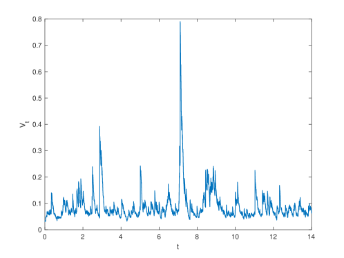
Figure 2: Simulation of the variance process $V$.

3 Affine characteristics

In this section, we give the joint Laplace transform of the log-price, the variance and its integrated process according to Duffie et al. [13, 14] and Keller-Ressel [33]. We begin by discussing the probability change between the historical and the risk-neutral pricing probability measures. We shall also make comparisons with several other affine models in literature.

3.1 Change of probability measures

We have assumed that model dynamics (1), (2) and (4) are specified under a risk-neutral probability $\mathbb{Q}$. However, it is important to establish a link with the physical or historical one generally denoted by $\mathbb{P}$ in order to keep a tractable form for the evolution of the processes describing the market. The construction of an equivalent historical probability is based on an Esscher-type transformation in Kallsen et al. [31] which is a natural extension of the class proposed by Heston [27]. The next result shows that the general class of temperated Heston-type model is closed under the change of probability and is a slight modification of [30, Proposition 4.1].

Proposition 3.1

Let $(S,V)$ be as in (1) and (2) under the probability measure $\mathbb{Q}$ and assume that the filtration $\mathbb{F}$ is generated by the random fields $(W,\overline{W})$ and $\widetilde{N}$. Fix $(\eta,\overline{\eta})\in\mathbb{R}^{2}$ and $\theta\in\mathbb{R}_{+}$, and define

$$U_{t}:=\eta\int_{0}^{t}\int_{0}^{V_{s}}W(ds,du)+\overline{\eta}\int_{0}^{t}\int_{0}^{V_{s}}\overline{W}(ds,du)+\int_{0}^{t}\int_{0}^{V_{s-}}\int_{0}^{\infty}(e^{-\theta\zeta}-1)\widetilde{N}(ds,du,d\zeta).$$

Then the Doléans-Dade exponential $\mathcal{E}(U)$ is a martingale and the probability measure $\mathbb{P}$ defined by

$$\left.\frac{d\mathbb{P}}{d\mathbb{Q}}\right|_{\mathcal{F}_{t}}=\mathcal{E}(U)_{t},$$

is equivalent to $\mathbb{Q}$. Moreover, under $\mathbb{P}$, $(S,V)$ satisfy (1) and (2) with the parameters $\sigma^{\mathbb{P}}=\sigma$, $\sigma^{\mathbb{P}}_{N}=\sigma_{N}$,

$$a^{\mathbb{P}}=a-\sigma\eta-\frac{\alpha\sigma_{N}}{\cos(\pi\alpha/2)}\theta^{\alpha-1},\quad b^{\mathbb{P}}=ab/a^{\mathbb{P}},$$

and the Lévy measure

$$\nu_{\alpha}^{\mathbb{P}}(d\zeta)=-\frac{1_{\{\zeta>0\}}e^{-\theta\zeta}}{\cos(\pi\alpha/2)\Gamma(-\alpha)\zeta^{1+\alpha}}d\zeta.$$

The model under $\mathbb{P}$ remains in the CBI class of $\alpha$-Heston model and shares similar behaviors. Note that the parameters $\eta,\overline{\eta}$ and $\theta$ are chosen such that $a^{\mathbb{P}}\in\mathbb{R}_{+}$. As a direct consequence of the above proposition, the return rate of the price process under $\mathbb{P}$ becomes

$$\mu^{\mathbb{P}}_{t}=r-V_{t}\left(\rho\eta+\sqrt{1-\rho^{2}}\overline{\eta}\right).$$

The risk premiums are given by

$$\lambda_{S}(t) := \mu_{t}^{\mathbb{P}}-r=-\left(\rho\eta+\sqrt{1-\rho^{2}}\overline{\eta}\right)V_{t}$$

$$\lambda_{V}(t) := (a^{\mathbb{P}}-a)V_{t}=-\left(\sigma\eta+\frac{\alpha\sigma_{N}}{\cos(\pi\alpha/2)}\theta^{\alpha-1}\right)V_{t}\,.$$

When $\eta<0$, the risk premium $\lambda_{V}$ is positively correlated with the volatility process $V$. The positive correlation between the risk premium and the volatility can explain the strongly upward sloping in VIX smile detailed in [6].

3.2 Joint characteristic function

In the Heston model, it is well known that the characteristic function plays a crucial role for the pricing of derivatives and the model calibration. We now provide the joint Laplace transform of the triplet: the log-price, the variance and its integrated process. The following result is a direct consequence of [13] and [33] and its proof is postponed to Appendix.

Proposition 3.2

Let $Y_{t}=\log S_{t}$. For any $\xi=(\xi_{1},\xi_{2},\xi_{3})\in i\mathbb{R}\times\mathbb{C}_{-}^{2}$,

$$\mathbb{E}\Big{[}\exp\big{(}\xi_{1}Y_{t}+\xi_{2}V_{t}+\xi_{3}\int_{0}^{t}V_{s}ds\big{)}\Big{]}=\exp\Big{(}\xi_{1}Y_{0}+\psi(t,\xi)V_{0}+\phi(t,\xi)\Big{)}$$ (8)

where $\phi$ and $\psi$ solve the generalized Riccati equations

$$\partial_{t}\phi(t,\xi) =F(\xi_{1},\psi(t,\xi),\xi_{3}),\quad\phi(0,\xi)=0;$$ (9)

$$\partial_{t}\psi(t,\xi) =R(\xi_{1},\psi(t,\xi),\xi_{3}),\quad\psi(0,\xi)=\xi_{2}.$$ (10)

Moreover, the functions $F$ and $R:i\mathbb{R}\times\mathbb{C}_{-}^{2}\rightarrow\mathbb{R}$ are defined by

$$F(\xi_{1},\xi_{2},\xi_{3}) = r\xi_{1}+ab\xi_{2},$$ (11)

$$R(\xi_{1},\xi_{2},\xi_{3}) = \frac{1}{2}(\xi_{1}^{2}-\xi_{1})+\rho\sigma\xi_{1}\xi_{2}+\frac{1}{2}\sigma^{2}\xi_{2}^{2}-a\xi_{2}-\frac{\sigma_{N}^{\alpha}}{\cos(\pi\alpha/2)}(-\xi_{2})^{\alpha}+\xi_{3}.$$ (12)

To compare the $\alpha$-Heston model with other models in literature, we consider in the remaining of the paper the usual case as in [13] and [33] where the third vaiable $\xi_{3}$ is omitted and $r=0$. Recall that in the standard Heston model, the generalized Riccati operators are given by

$$F_{H}(\xi_{1},\xi_{2})=ab\xi_{2},\quad{\text{and }}\quad R_{H}(\xi_{1},\xi_{2})=\frac{1}{2}(\xi_{1}^{2}-\xi_{1})+\rho\sigma\xi_{1}\xi_{2}+\frac{1}{2}\sigma^{2}\xi_{2}^{2}-a\xi_{2}.$$ (13)

By Proposition 3.2, the $\alpha$-Heston model admits

$$F(\xi_{1},\xi_{2})=F_{H}(\xi_{1},\xi_{2}),\quad{\text{and }}\quad R(\xi_{1},\xi_{2})=R_{H}(\xi_{1},\xi_{2})-\frac{\sigma_{N}^{\alpha}}{\cos(\pi\alpha/2)}(-\xi_{2})^{\alpha}.$$ (14)

Note that the function $R$ in (14) is not analytic and is well defined only for $\xi_{2}\leq 0$. The difference $R(\xi_{1},\xi_{2})-R_{H}(\xi_{1},\xi_{2})$ is positive since $\cos(\pi\alpha/2)<0$ for $\alpha\in(1,2]$. As stated in [33], $F$ characterizes the state-independent dynamic of $(S,V)$ while R characterizes the state-dependent dynamic. In order to highlight the primacy of function $\psi$ in (10), we refer $R$ as the main generalized Riccati operator.

The main point we highlight is that many models discussed in literature admit similar forms of $R$. In Barndorff-Nielsen and Shephard [4], $R$ is a particular case of Heston one, i.e. $\sigma=0$, and the main innovation of their model is to extend in an interesting way the auxiliary operator $F$. The model in Bates [5] has a more general generalized Riccati operator $R$ but the new term depends only on the Laplace coefficient of the stock $S$. So the variance process in [5] follows the CIR diffusion and hence there is no difference for volatility and variance options compared to Heston model. For the stochastic volatility jump model in Nicolato et al. [40], the examples share the same Riccati operator of the Heston model. As a consequence, the Laplace transform of the variance process has a certain form for the affine function. Then, it is not surprising that “the specific choice of jump distribution has a minor effect on the qualitative behavior of the skew and the term structure of the implied volatility surface” as noted in [40] (see also [39]), since the plasticity of the model is limited to the form of the auxiliary function $\phi(t,\xi)$ which is independent of the level of initial variance $V_{0}$ in the cumulant generating function.

Our model exhibits a different behavior due to the supplementary $\alpha$-power term appearing in the main generalized Riccati operator $R$, which adds more flexibility to the coefficient of the variance $\psi(t,\xi)$ in the cumulant generating function. The reason lies in the fact that the new jump part depends on the variance itself, resulting in a non-linear dependence in (12). In other words, the self-exciting property of jump term introduces a completely different shape of cumulant generating function.

4 Asymptotic behaviors and implied volatility

In this section, we focus on the implied volatility surfaces for both asset and variance options, in particular, on their asymptotic behaviors at small or large strikes. We follow the model-free result in the pioneering paper of Lee [34] and aim to obtain some refinements for the specific $\alpha$-Heston model. We also provide the moment explosion conditions.

4.1 Asset options

We begin by providing the following results on the generalized Riccati operator $R$ by [33] and give the moment explosion condition for the asset price $S$.

Proposition 4.1

We assume $a>\sigma\rho$. Define $w(\xi_{1})$ such that $R(\xi_{1},w(\xi_{1}))=0$ and $T_{*}(u):=\sup\{T:\,\mathbb{E}[S_{T}^{u}]<\infty\}$

1. $w(\xi_{1})$ has $[0,1]$ as maximal support.

2. $\forall\xi_{1}\in[0,1]$ we have $\lim_{t\rightarrow\infty}\phi(t,\xi_{1},w)=w(\xi_{1})$.

3. $\forall\xi_{1}\in[0,1]$ we have $T_{*}(\xi_{1})=\infty$ and $\forall\xi_{1}\notin[0,1]$ we have $T_{*}(\xi_{1})=0$.

Proof.

The couple $(Y_{t},V_{t})$ is an affine process characterized by (14) and $F(u,w):=abw$. Note that $F(0,0)=R(0,0)=R(1,0)=0$ and $\chi(q_{1}):=\frac{\partial R(q_{1},q_{2})}{\partial q_{2}}\big{|}_{q_{2}=0}=\rho\sigma q_{1}-a<\infty$. Then by Keller-Ressel [33, Corollary 2.7] we have $\mathbb{E}[S_{T}]<\infty$ for any $T>0$. Also note that $\chi(0)<0$ and $\chi(1)<0$ as $a>0$, $\rho<0$ and $\sigma>0$. It follows from [33, Lemma 3.2] that there exist a maximal interval $I$ and a unique function $w\in C(I)\cap C^{1}(I^{\circ})$ such that $R(q_{1},w(q_{1}))=0$ for all $q_{1}\in I$ with $w(0)=w(1)=0$. Since $0=\sup\{q_{2}\geq 0:R(q_{1},q_{2})<\infty\}$, $R(q_{1},q_{2})>0$ if $q_{1}<0$ and $q_{2}<0$, and $R(q_{1},0)=\frac{1}{2}q_{1}(q_{1}-1)$, we immediately have that $I=[0,1]$. Then the set $\{q_{1}\in I:F(q_{1},w(q_{1}))<\infty\}$ coincide with $[0,1]$. By [33, Theorem 3.2] we have $\mathbb{E}[S_{T}^{q}]=\infty$ for any $q\in\mathbb{R}\setminus[0,1]$. $\Box$

Corollary 4.2

The above proposition implies that for any $T>0$, we have

$$\sup\{p>0:\mathbb{E}[S_{T}^{p}]<\infty\}=1\quad\mbox{and}\quad\sup\{p>0:\mathbb{E}[S_{T}^{-p}]<\infty\}=0.$$

In other words, the maximal domain of moment generating function $\mathbb{E}[e^{q\log S_{T}}]$ is $[0,1]$.

Let $\Sigma_{S}(T,k)$ be the implied volatility of a call option written on the asset price $S$ with maturity $T$ and strike $K=e^{k}$. Then combined with a model-free result of Lee [34], known as the moment formula, it yields that the asymptotic behavior of the implied volatility at extreme strikes is given by

$$\limsup_{k\rightarrow\pm\infty}\frac{\Sigma_{S}^{2}(T,k)}{|k|}=\frac{2}{T},$$ (15)

which means that the wing behavior of implied volatility for the asset options is the sharpest possible one by [34, Theorem 3.2 and 3.4].

In the following of this subsection, we study the probability tails of $S$ which allows to replace the “$\limsup$” by the usual limit in (15) for the left wing of the asset options. The next technical lemma, whose proof is postponed to Appendix, shows that the extremal behavior of $V$ is mainly due to one large jump of the driving processes $Z$.

Lemma 4.3

Fix $T>0$ and consider the variance process $V$ defined by (4). Then there exists a nonzero boundedly finite measure $\delta$ on $\mathscr{B}(\bar{D}_{0}[0,T])$ with $\delta(\bar{D}_{0}[0,T]\backslash D[0,T])=0$ such that, as $u\rightarrow\infty$,

$$u^{\alpha}\mathbb{P}({V}/u\in\cdot)\overset{\widehat{w}}{\longrightarrow}\delta(\cdot)\quad on\quad\mathscr{B}(\bar{D}_{0}([0,T]),$$ (16)

where $\delta$ is given by:

$$\delta(\cdot)=\sigma_{N}^{\alpha}\int_{0}^{T}\big{(}b(1-e^{-as})+xe^{-as}\big{)}\int_{0}^{\infty}\mathbb{E}\Big{[}1_{\big{\{}w_{t}:=e^{-a(t-s)}y1_{[s,T]}(t)\in\;\cdot\;\big{\}}}\Big{]}\nu_{\alpha}(dy)ds,$$

and $\nu_{\alpha}$ is defined by (6). We refer to Hult and Lindskog [28, page 312] for the definition of $\bar{\mathbb{D}}_{0}[0,T]$ and the vague convergence $\overset{\rm\widehat{w}}{\longrightarrow}$.

Proposition 4.4

Fix $t>0$. For any $x\geq 0$, we have that

$$\mathbb{P}_{x}(-\log S_{t}>u)\sim-\Big{(}\frac{\sigma_{N}}{2a}\Big{)}^{\alpha}\frac{\iota_{\alpha}(t)}{\alpha\cos(\pi\alpha/2)\Gamma(-\alpha)}u^{-\alpha},\quad u\rightarrow+\infty,$$ (17)

where

$$\iota_{\alpha}(t)=e^{-\alpha at}\int_{0}^{t}(b(1-e^{-as})+xe^{-as})(e^{at}-e^{as})^{\alpha}ds.$$

Proof.

We have by (4) that

$$\log S_{t}=\log s_{0}+\int_{0}^{t}(r-\frac{1}{2}V_{s})ds+\int_{0}^{t}\sqrt{V_{s}}dB_{s}.$$ (18)

For any $t>0$, consider the asymptotic behavior of the probability tail for $\int_{0}^{t}V_{s}ds$, that is, $\mathbb{P}_{x}(\frac{1}{2}\int_{0}^{t}V_{s}ds>x)$. By Lemma 4.3, as $u\rightarrow+\infty$,

$$u^{\alpha}\mathbb{P}({V}/u\in\cdot)\overset{\widehat{w}}{\longrightarrow}\delta(\cdot)\quad on\quad\mathscr{B}(\bar{D}_{0}[0,t]),$$

Define the functional $h:\bar{D}_{0}[0,t]\longrightarrow\mathbb{R}_{+}$ by $h(w)=\frac{1}{2}\int_{0}^{t}w_{s}ds$. Let Disc($h$) be the set of discontinuities of $h$. By the definition of $h$ by (16), it is easy to see that $\delta({\rm Disc}(h))=0$. It follows from [28, Theorem 2.1] that as $u\rightarrow+\infty$,

$$u^{\alpha}\mathbb{P}_{x}\Big{(}\frac{1}{2u}\int_{0}^{t}V_{s}ds\in\cdot\Big{)}\overset{v}{\longrightarrow}\delta\circ h^{-1}(\cdot)\quad on\quad\mathscr{B}(\mathbb{R}_{+}),$$

and

$$\delta\circ h^{-1}(\cdot) = \sigma_{N}^{\alpha}\int_{0}^{t}\mathbb{E}[V_{s}]\int_{0}^{\infty}1_{\{\frac{y}{2}\int_{s}^{t}e^{-a(\zeta-s)}d\zeta\ \in\cdot\ \}}\nu_{\alpha}(dy)ds.$$

Thus we have that

$$\mathbb{P}_{x}\Big{(}\frac{1}{2}\int_{0}^{t}V_{s}ds>u\Big{)}\sim-\Big{(}\frac{\sigma_{N}}{2a}\Big{)}^{\alpha}\frac{\iota_{\alpha}(t)}{\alpha\cos(\pi\alpha/2)\Gamma(-\alpha)}u^{-\alpha},\quad u\rightarrow+\infty.$$

Furthermore we note that

$$\mathbb{E}_{x}\Big{[}\Big{(}\int_{0}^{t}\sqrt{V_{s}}dB_{s}\Big{)}^{2}\Big{]}=\int_{0}^{t}\mathbb{E}_{x}[V_{s}]ds<\infty.$$

In view of (18), we have that

$$\mathbb{P}_{x}(-\log S_{t}>u)\sim\mathbb{P}_{x}\Big{(}\frac{1}{2}\int_{0}^{t}V_{s}ds>u\Big{)},\quad u\rightarrow+\infty.$$

$\Box$

Corollary 4.5

Let $\Sigma_{S}(T,k)$ be the implied volatility of the option written on the stock price $S$ with maturity $T$ and strike $K=e^{k}$. Then the left wing of $\Sigma_{S}(T,k)$ has the following asymptotic shape as $k\rightarrow-\infty$:

$$\frac{\sqrt{T}\Sigma_{S}(T,k)}{\sqrt{2}} = \sqrt{-k+\alpha\log(-k)-\frac{1}{2}\log\log(-k)}$$ (19)

$$-\sqrt{\alpha\log(-k)-\frac{1}{2}\log\log(-k)}+O((\log(-k))^{-1/2}).$$

Proof.

Without loss of generality we assume $k<0$. Note that the put option price can be written as

$$P(e^{k}):=\mathbb{E}[(e^{k}-S_{T})_{+}]=\int_{-k}^{\infty}\mathbb{P}_{x}(-\log S_{T}>u)e^{-u}du.$$

By Proposition 4.4, it is not hard to see that

$$P(e^{k})\sim-\Big{(}\frac{\sigma_{N}}{2a}\Big{)}^{\alpha}\frac{\iota_{\alpha}(t)}{\alpha\cos(\pi\alpha/2)\Gamma(-\alpha)}e^{k}k^{-\alpha},\quad k\rightarrow-\infty.$$

Then (19) follows from the above asymptotic equality and [25, Theorem 3.7]. $\Box$

Figure 3 presents the implied volatility curves of the asset options. We use a Monte Carlo method with $10^{5}$ trajectories with the parameters $V_{0}=0.0332$, $a=5$, $b=0.144$, $\sigma=0.08$ and $\sigma_{N}=1$ coherent with the ones of Nicolato et al. [40]

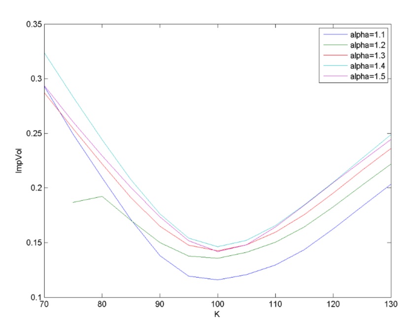
Figure 3: Implied volatilites for asset options

4.2 Variance options

We now consider the volatility and variance options for which a large growing literature has been developed (see for instance [22], [40] and [42]). In particular, it is highlighted in [42] and [40] about the upward-sloping implied volatility skew of VIX options. In the following, we derive the asymptotic behavior of tail probability of $V$, which will imply the moment explosion condition for $V$ and the extreme behaviors of the variance options. We begin by giving two technical lemmas.

Lemma 4.6

Let $X$ be a positive random variable.

1. (Karamata Tauberian Theorem [7, Theorem 1.7.1]) For constants $C>0$, $\beta>0$ and a slowly varying function (at infinity) $L$,

   $$\mathbb{E}[e^{-\lambda X}]\sim C\lambda^{-\beta}L(\lambda),\quad\mbox{as}\quad\lambda\rightarrow\infty,$$

   if and only if

   $$\mathbb{P}(X\leq u)\sim\frac{C}{\Gamma(1+\beta)}u^{\beta}L(1/u),\quad\mbox{as}\quad u\rightarrow 0^{+}.$$

2. (de Bruijn’s Tauberian Theorem [8, Theorem 4]) Let $0\leq\beta\leq 1$ be a constant, $L$ be a slowly varying function at infinity, and $L^{*}$ be the conjugate slowly varying function to $L$. Then

   $$\log\mathbb{E}[e^{-\lambda X}]\sim-\lambda^{\beta}/L(\lambda)^{1-\beta}\quad\mbox{as}\ \lambda\rightarrow\infty,$$

   if and only if

   $$\log\mathbb{P}(X\leq u)\sim-(1-\beta)\beta^{\beta/(1-\beta)}u^{-\beta/(1-\beta)}L^{*}(u^{-1/(1-\beta)})\quad\mbox{as}\ u\rightarrow 0^{+}.$$

Lemma 4.7

For any $0<\beta<\alpha$, there exists a locally bounded function $C(\cdot)\geq 0$ such that for any $T\geq 0$,

$$\mathbb{E}_{x}\Big{[}\sup_{0\leq t\leq T}V_{t}^{\beta}\Big{]}\leq C(T)(1+x^{\beta}).$$

Proposition 4.8

(probability tails of $V_{t}$) Fix $t>0$. For any $x\geq 0$, we have that

$$\mathbb{P}_{x}(V_{t}>u)\sim-\frac{\sigma_{N}^{\alpha}}{\alpha\Gamma(-\alpha)\cos(\pi\alpha/2)}\big{(}q_{\alpha}(t)+p_{\alpha}(t)x\big{)}u^{-\alpha},\quad\mbox{as}\quad u\to\infty,$$ (20)

where

$$~{}p_{\alpha}(t)=\frac{1}{a(\alpha-1)}\left(e^{-at}-e^{-\alpha at}\right),\quad q_{\alpha}(t)=b\left(\frac{1}{\alpha a}(1-e^{-\alpha at})-p_{\alpha}(t)\right).$$

Furthermore,

1. if $\sigma>0$, then

   $$\mathbb{P}_{x}(V_{t}\leq u)\sim u^{2ab/\sigma^{2}}\frac{\bar{v}_{t}^{2ab/\sigma^{2}}}{\Gamma\left(1+{2ab}/{\sigma^{2}}\right)}\exp\Big{(}-x\bar{v}_{t}-ab\int_{\bar{v}_{t}}^{\infty}\Big{(}\frac{z}{\Psi_{\alpha}(z)}-\frac{2}{\sigma^{2}z}\Big{)}dz\Big{)},\,\mbox{as}\,\,u\to 0,$$ (21)

   where $\bar{v}_{t}$ is the minimal solution of the ODE

   $$\frac{d}{dt}\bar{v}_{t}=-\Psi_{\alpha}(\bar{v}_{t}),\quad t>0,$$ (22)

   with singular initial condition $\bar{v}_{0+}=\infty$;

2. if $\sigma=0$, then

   $$\log\mathbb{P}_{x}(V_{t}\leq u)\sim-\frac{\alpha-1}{2-\alpha}\left(-ab\cos\big{(}\frac{\pi\alpha}{2}\big{)}\right)^{\frac{1}{\alpha-1}}\sigma_{N}^{-\frac{\alpha}{\alpha-1}}u^{-\frac{2-\alpha}{\alpha-1}},\quad\mbox{as}\quad u\rightarrow 0.$$ (23)

Proof.

We have by (4) that

$$V_{t}=e^{-at}V_{0}+ab\int_{0}^{t}e^{-a(t-s)}ds+\sigma\int_{0}^{t}e^{-a(t-s)}\sqrt{V_{s}}dB_{s}+\sigma_{N}\int_{0}^{t}e^{-a(t-s)}V_{s-}^{1/\alpha}dZ_{s}.$$ (24)

Note that $\mathbb{E}_{x}[V_{t}]=e^{-at}x+b(1-e^{-at})$. By Markov’s inequality,

$$\mathbb{P}_{x}\Big{(}\Big{|}\int_{0}^{t}e^{-a(t-s)}\sqrt{V_{s}}dB_{s}\Big{|}>u\Big{)} \leq u^{-2}\mathbb{E}_{x}\Big{[}\int_{0}^{t}e^{-2a(t-s)}V_{s}ds\Big{]}$$ (25)

$$\leq \Big{(}\frac{x}{a}+bt\Big{)}u^{-2}.$$

It follows from Lemma 4.7 that $\mathbb{E}[\sup_{0\leq t\leq T}(\sqrt[\alpha]{V_{t}})^{\alpha+\delta}]<\infty$ for $0<\delta<\alpha(\alpha-1)$. Then by Hult and Lindskog [28, Theorem 3.4], we have as $u\rightarrow\infty$,

$$\mathbb{P}_{x}\Big{(}\sigma_{N}\int_{0}^{t}e^{-a(t-s)}V_{s-}^{1/\alpha}dZ_{s}>u\Big{)} \sim \nu_{\alpha}(u,\infty)\sigma_{N}^{\alpha}\int_{0}^{t}e^{-\alpha a(t-s)}\mathbb{E}_{x}[V_{s}]ds$$ (26)

$$\sim -\frac{\sigma_{N}^{\alpha}}{\alpha\cos(\pi\alpha/2)\Gamma(-\alpha)}\big{(}q_{\alpha}(t)+p_{\alpha}(t)x\big{)}u^{-\alpha}.$$

In view of (24), (25) and (26), the extremal behavior of $V_{t}$ is determined by the forth term on the right-hand side of (24). Then we have, as $u\rightarrow\infty$,

$$\mathbb{P}_{x}(V_{t}>u) \sim \mathbb{P}_{x}\Big{(}\sigma_{N}\int_{0}^{t}e^{-a(t-s)}V_{s-}^{1/\alpha}dZ_{s}>u\Big{)},$$

which gives (20). On the other hand, by Proposition 3.2 we have

$$\mathbb{E}_{x}\left[e^{-\lambda V_{t}}\right]=\exp\Big{(}-xv_{t}(\lambda)-ab\int_{0}^{t}v_{s}(\lambda)ds\Big{)},$$

where $v_{t}(\lambda)$ is the unique solution of the following ODE:

$$\frac{\partial v_{t}(\lambda)}{\partial t}=-\Psi_{\alpha}(v_{t}(\lambda)),\quad v_{0}(\lambda)=\lambda.$$ (27)

It follows from [35, Theorem 3.5, 3.8, Corollary 3.11] that $\bar{v}_{t}=\uparrow\lim_{\lambda\rightarrow\infty}v_{t}(\lambda)$ exists in $(0,\infty)$ for all $t>0$, and $\bar{v}_{t}$ is the minimal solution of the singular initial value problem (22).

First consider the case of $\sigma>0$. By (27),

$$\int_{0}^{t}v_{s}(\lambda)ds=\int_{v_{t}(\lambda)}^{\lambda}\frac{u}{\Psi_{\alpha}(u)}du=\int_{v_{t}(\lambda)}^{\lambda}\frac{2}{\sigma^{2}u}du+\int_{v_{t}(\lambda)}^{\lambda}\Big{(}\frac{u}{\Psi_{\alpha}(u)}-\frac{2}{\sigma^{2}u}\Big{)}du,\quad\lambda>0,\ t>0.$$

Note that $\frac{2}{\sigma^{2}u}-\frac{u}{\Psi_{\alpha}(u)}=O(u^{-(3-\alpha)})$ as $u\rightarrow\infty$ and thus $0<\int_{\bar{v}_{t}}^{\infty}\Big{(}\frac{2}{\sigma^{2}u}-\frac{u}{\Psi_{\alpha}(u)}\Big{)}du<\infty$. A simple calculation shows that

$$\mathbb{E}_{x}\left[e^{-\lambda V_{t}}\right]\sim\bar{v}_{t}^{2ab/\sigma^{2}}\lambda^{-2ab/\sigma^{2}}\exp\left(-x\bar{v}_{t}-ab\int_{\bar{v}_{t}}^{\infty}\Big{(}\frac{u}{\Psi_{\alpha}(u)}-\frac{2}{\sigma^{2}u}\Big{)}du\right),\quad\lambda\rightarrow 0.$$

Then Karamata Tauberian Theorem (see Lemma 4.6 (i)) gives (21).

Now we turn to the case of $\sigma=0$. Denote by $\sigma_{1}=-\frac{\sigma_{N}^{\alpha}}{\cos(\pi\alpha/2)}$. Recall that $\bar{v}_{t}=\uparrow\lim_{\lambda\rightarrow\infty}v_{t}(\lambda)\in(0,\infty),$ which is the minimal solution of the singular initial value problem (22) with $\sigma=0$. Still by (27),

$$\log\mathbb{E}_{x}\left[e^{-\lambda V_{t}}\right]=-xv_{t}(\lambda)-ab\int_{v_{t}(\lambda)}^{\lambda}\frac{1}{a+\sigma_{1}\lambda^{\alpha-1}}du\sim\frac{ab}{\alpha-2}\frac{\lambda}{a+\sigma_{1}\lambda^{\alpha-1}}\sim\frac{ab}{\sigma_{1}(\alpha-2)}\lambda^{2-\alpha}.$$

Then de Bruijn’s Tauberian Theorem (see Lemma 4.6 (ii)) gives (23). $\Box$

Corollary 4.9

As a consequence of Proposition 4.8, we have, for any $\alpha\in(1,2)$,

$$\{p\in\mathbb{R}:\mathbb{E}[V_{t}^{p}]<\infty\}=\big{(}-\frac{2ab}{\sigma^{2}},\alpha\big{)}$$ (28)

where by convention $2ab/\sigma^{2}=+\infty$ if $\sigma=0$.

Proof.

By integration by parts, we have, for $p>0$,

$$\mathbb{E}[V_{t}^{p}]=-\lim_{u\rightarrow\infty}u^{p}\mathbb{P}(V_{t}>u)+p\int_{0}^{\infty}u^{p-1}\mathbb{P}(V_{t}>u)du.$$

By Proposition 4.8, $\mathbb{P}(V_{t}>u)\sim C(t)u^{-\alpha}$ as $u\rightarrow\infty$ for some function $C(t)$. Then we obtain $\mathbb{E}[V_{t}^{p}]<\infty$ for $0\leq p<\alpha$ and $\mathbb{E}[V_{t}^{p}]=\infty$ for $p\geq\alpha$. Similarly, we consider $\mathbb{E}[(1/V_{t})^{p}]$ and have $\mathbb{P}(1/V_{t}>u)\sim D(t)u^{-2ab/\sigma^{2}}$ as $u\rightarrow\infty$. Then we obtain $\mathbb{E}[(1/V_{t})^{p}]<\infty$ for $0\leq p<2ab/\sigma^{2}$ and $\mathbb{E}[(1/V_{t})^{p}]=\infty$ if $p\geq 2ab/\sigma^{2}$. $\Box$

Corollary 4.10

Let $\Sigma_{V}(T,k)$ be the implied volatility of call option written on the variance process $V$ with maturity $T$ and strike $K=e^{k}$ and let $\psi(q)=2-4(\sqrt{q^{2}+q}-q)$. Then the right wing of $\Sigma_{V}(T,k)$ has the following asymptotic shape:

$$\Sigma_{V}(T,k)\sim\Big{(}\frac{\psi(\alpha)}{T}\Big{)}^{1/2}\sqrt{k},\quad k\rightarrow+\infty$$ (29)

The left wing satisfies

1. if $\sigma>0$, then

   $$\Sigma_{V}(T,k)\sim\Big{(}\frac{\psi(\frac{2ab}{\sigma^{2}})}{T}\Big{)}^{1/2}\sqrt{-k},\quad k\rightarrow-\infty;$$ (30)

2. if $\sigma=0$, then

   $$\Sigma_{V}(T,k)\sim\frac{1}{\sqrt{2T}}(-k)\Big{(}\log\frac{e^{k}}{P(e^{k})}\Big{)}^{1/2},\quad k\rightarrow-\infty.$$ (31)

   where $P(e^{k})=E[(e^{k}-V_{T})^{+}]$.

Proof.

Combining (20) and [40, Proposition 2.2-(a)], we obtain directly (29). Similarly, (21) and [40, Proposition 2.4-(a)] leads to (30). In the case where $\sigma=0$, (23) implies that $\sup\{p>0:\mathbb{E}[V_{t}^{-p}]<\infty\}=\infty$. Then (31) follows from [40, Theorem 2.3-(iii)]. $\Box$

Corollary 4.10 gives the explicit behavior of the implied volatility of variance options with extreme strikes far from the moneyness. We note that the right wing depends only on the parameter $\alpha$ which is the characteristic parameter of the jump term. When $\alpha$ decreases, the tail becomes heavier and the slope in (29) increases. In contrast, the left wing depends on the parameters which belong to the pure CIR part with Brownian diffusion and the explaining coefficient $2ab/\sigma^{2}$ in (30) is linked to the Feller condition. When the Brownian term disappears, i.e. $\sigma=0$, then there occurs a discontinuity on the left wing behavior of the variance volatility surface.

5 Jump cluster behaviour

In this section, we study the jump cluster phenomenon by giving a decomposition formula of the variance process $V$ and we analyze some properties of the cluster processes.

5.1 Cluster decomposition of the variance process

Let us fix a jump threshold ${y}=\sigma_{Z}\overline{y}$ and denote by $\{\tau_{n}\}_{n\geq 1}$ the sequence of jump times of $V$ whose sizes are larger than $y$. We call $\{\tau_{n}\}_{n\geq 1}$ the large jumps. By separating the large and small jumps, the variance process (2) can be written as

$$\begin{array}[]{rcl}\displaystyle V_{t}&\displaystyle=V_{0}&\displaystyle+\int_{0}^{t}a\left(b-\frac{\sigma_{N}\Theta(\alpha,y)V_{s}}{a}-V_{s}\right)ds+\sigma\int_{0}^{t}\int_{0}^{V_{s}}W(ds,du)\\ &&\displaystyle+\sigma_{N}\int_{0}^{t}\int_{0}^{V_{s-}}\int_{0}^{\overline{y}}\zeta\widetilde{N}(ds,du,d\zeta)++\sigma_{N}\int_{0}^{t}\int_{0}^{V_{s-}}\int_{\overline{y}}^{\infty}\zeta{N}(ds,du,d\zeta)\end{array}$$ (32)

where

$$\Theta(\alpha,y) = \int_{\overline{y}}^{\infty}\zeta\nu_{\alpha}(d\zeta)=\frac{2}{\pi}\alpha\Gamma(\alpha-1)\sin\left(\frac{\pi\alpha}{2}\right)\overline{y}^{1-\alpha}.$$ (33)

We denote by

$$\widetilde{a}(\alpha,y)=a+\sigma_{N}\Theta(\alpha,y)\quad\text{ and }\quad\widetilde{b}(\alpha,y)=\frac{ab}{a+\sigma_{N}\Theta(\alpha,y)}.$$

Then between two large jumps times, that is, for any $t\in[\tau_{n},\tau_{n+1})$, we have

$$\begin{array}[]{rcl}\displaystyle V_{t}&\displaystyle=V_{\tau_{n}}&\displaystyle+\int_{\tau_{n}}^{t}\widetilde{a}(\alpha,y)\big{(}\widetilde{b}(\alpha,y)-V_{s}\big{)}ds+\sigma\int_{\tau_{n}}^{t}\int_{0}^{V_{s}}W(ds,du)\\ &&\displaystyle+\sigma_{N}\int_{\tau_{n}}^{t}\int_{0}^{V_{s-}}\int_{0}^{\overline{y}}\zeta\widetilde{N}(ds,du,d\zeta).\end{array}$$ (34)

The expression (34) shows that two phenomena arise between two large jumps. First, the mean long-term level $b$ is reduced. This effect is standard since the mean level $\widetilde{b}(\alpha,y)$ becomes lower to compensate the large jumps in order to preserve the global mean level $b$. Second and more surprisingly, the mean reverting speed $a$ is augmented. That is, the volatility decays more quickly between two jumps. Moreover, this speed is greater when the parameter $\alpha$ decreases and tends to infinity as $\alpha$ approaches $1$ since $\Theta(\alpha,y)\sim(\alpha-1)^{-1}$.

We introduce the truncated process of $V$ up to the jump threshold, which will serve as the fundamental part in the decomposition, as

$$\begin{split}{V}^{(y)}_{t}=V_{0}&+\int_{0}^{t}\widetilde{a}(\alpha,y)\big{(}\widetilde{b}(\alpha,y)-{V}_{s}^{(y)}\big{)}ds+\sigma\int_{0}^{t}\int_{0}^{{V}_{s}^{(y)}}W(ds,du)\\ &+\sigma_{N}\int_{0}^{t}\int_{0}^{{V}_{s-}^{(y)}}\int_{0}^{\overline{y}}\zeta\widetilde{N}(ds,du,d\zeta),\quad t\geq 0.\end{split}$$ (35)

Similar as $V$, the process $V^{(y)}$ is also a CBI process. By definition, the jumps of the process $V^{(y)}$ are all smaller than $y$. In addition, $V^{(y)}$ coincides with $V$ before the first large jump $\tau_{1}$. The next result studies the first large jump and its jump size, which will be useful for the decomposition.

Lemma 5.1

We have

$$\mathbb{P}(\tau_{1}>t)=\mathbb{E}\Big{[}\exp{\Big{\{}-\Big{(}\int_{\overline{y}}^{\infty}\mu_{\alpha}(d\zeta)\Big{)}\Big{(}\int_{0}^{t}{V}^{(y)}_{s}ds\Big{)}\Big{\}}}\Big{]}.$$ (36)

The jump $\Delta V_{\tau_{1}}:=V_{\tau_{1}}-V_{\tau_{1}-}$ is independent of $\tau_{1}$ and $V^{(y)}$, and satisfies

$$\mathbb{P}(\Delta V_{\tau_{1}}\in d\zeta)=1_{\{\zeta>{y}\}}\,\frac{\alpha{y}^{\alpha}}{\zeta^{1+\alpha}}d\zeta.$$ (37)

It is not hard to see that $\mathbb{P}(V_{t}\geq V^{(y)}_{t},\forall t\geq 0)=1$. Then the large jump in (32) can be separated into two parts as

$$\int_{0}^{t}\int_{0}^{V_{s-}}\int_{\bar{y}}^{\infty}N(ds,du,d\zeta)=\int_{0}^{t}\int_{0}^{V^{(y)}_{s-}}\int_{\bar{y}}^{\infty}N(ds,du,d\zeta)+\int_{0}^{t}\int_{V^{(y)}_{s-}}^{V_{s-}}\int_{\bar{y}}^{\infty}N(ds,du,d\zeta).$$ (38)

Let

$$J_{t}^{(y)}=\int_{0}^{t}\int_{0}^{V^{(y)}_{s-}}\int_{\bar{y}}^{\infty}N(ds,du,d\zeta),\quad t\geq 0$$ (39)

which is a point process whose arrival times $\{T_{n}\}_{n\geq 1}$ coincide with part of the large jump times and those jumps are called the mother jumps. By definition, the mother jumps form a subset of large jumps. Each mother jump will induce a cluster process $v^{(n)}$ which starts from time $T_{n}$ with initial value $\Delta V_{T_{n}}=V_{T_{n}}-V_{T_{n}-}$ and is given recursively by

$$\begin{split}v_{t}^{(n)}=\Delta V_{T_{n}}&-a\int_{T_{n}}^{t}v^{(n)}_{s}ds+\sigma\int_{T_{n}}^{t}\int_{V^{(y)}_{s}+\sum_{i=1}^{n-1}v^{(i)}_{s}}^{V^{(y)}_{s}+\sum_{i=1}^{n}v^{(i)}_{s}}W(ds,du)\\ &+\sigma_{Z}\int_{T_{n}}^{t}\int_{V^{(y)}_{s-}+\sum_{i=1}^{n-1}v^{(i)}_{s-}}^{V^{(y)}_{s-}+\sum_{i=1}^{n}v^{(i)}_{s-}}\int_{\mathbb{R}^{+}}\zeta\widetilde{N}(ds,du,d\zeta),\quad t\in[T_{n},\infty).\end{split}$$ (40)

The next result provides the decomposition of $V$ as the sum of the fundamental process $V^{(y)}$ and a sequence of cluster processes. The decomposition form is inspired by Duquesne and Labbe [15].

Proposition 5.2

The variance process $V$ given by (2) has the decomposition:

$${V_{t}=V^{(y)}_{t}+\sum_{n=1}^{J^{(y)}_{t}}u_{t-T_{n}}^{(n)}},\quad t\geq 0,$$ (41)

where $u^{(n)}_{t}=v^{(n)}_{T_{n}+t}$ with $v^{(n)}$ given by (40). Moreover, we have that

1. $\{u^{(n)}:n=1,2,\cdots\}$ is the sequence of independent identically distributed processes and for each $n$, $u^{(n)}$ has the same distribution as an $\alpha$-$\mathrm{CIR}(a,0,\sigma,\sigma_{Z},\alpha)$ process given by

   $$u_{t}=u_{0}-a\int_{0}^{t}u_{s}ds+\sigma\int_{0}^{t}\sqrt{u_{s}}dB_{s}+\sigma_{N}\int_{0}^{t}\sqrt[\alpha]{u_{s-}}dZ_{s},$$ (42)

   where $u_{0}\overset{d}{=}\Delta V_{\tau_{1}}$ and its distribution is given by (37).

2. The pair $({V}^{(y)},J^{(y)})$ is independent of $\{u^{(n)}\}$. Conditional on ${V}^{(y)}$, $J^{(y)}$ is a time inhomogenous Poisson process with intensity function $\big{(}\int_{\bar{y}}^{\infty}\nu_{\alpha}(d\zeta)\big{)}{V}^{(y)}_{\cdot}$.

Note that each cluster process has the same distribution as an $\alpha$-square root jump process which is similar to (4) but with parameter $b=0$, that is, an $\alpha$-$\mathrm{CIR}(a,0,\sigma,\sigma_{Z},\alpha)$ process also known as a CB process without immigration. The jumps given by $(J_{t},t\geq 0)$ are called mother jumps in the sense that each mother jump $T_{n}$ will induce a cluster of jumps, or so-called son jumps, via its cluster (branching) process $u^{(n)}$. Conversely, any jump from $\big{(}\int_{0}^{t}\int_{V^{(y)}_{s-}}^{V_{s-}}\int_{\bar{y}}^{\infty}N(ds,du,d\zeta),t\geq 0\big{)}$ in (38), that is, a large jump but not mother jump, is a child jump of some mother jump.

5.2 The cluster processes

We finally focus on the cluster processes and present some of their properties. We are particularly interested in two quantities. The first one is the number of clusters before a given time $t$, which is equal to the number of mother jumps. The second one is the duration of each cluster process.

Proposition 5.3

1. The expected number of clusters during $[0,t]$ is

   $$\mathbb{E}[J_{t}^{(y)}]=\frac{(1-\alpha)\sigma_{Z}^{\alpha}}{\cos(\pi\alpha/2)\Gamma(2-\alpha)y^{\alpha}}\Big{(}\widetilde{b}(\alpha,y)t+\frac{V_{0}-\widetilde{b}(\alpha,y)}{\widetilde{a}(\alpha,y)}(1-e^{-\widetilde{a}(\alpha,y)t})\Big{)}.$$ (43)

2. Let $\theta_{n}:=\inf\{t\geq 0:u_{t}^{(n)}=0\}$ be the duration of the cluster $u^{(n)}$. We have $\mathbb{P}(\theta_{n}<\infty)=1$ and

   $$\mathbb{E}[\theta_{n}]=\alpha y^{\alpha}\int_{0}^{\infty}\frac{dz}{\Psi_{\alpha}(z)}\int_{y}^{\infty}\frac{1-e^{-\zeta z}}{\zeta^{1+\alpha}}d\zeta.$$ (44)

We note that the expected duration of all clustering processes are equal, which means that the initial value of $u^{(i)}$, that is, the jump size of the triggering mother jump has no impact on the duration. By (44), we have

$$\mathbb{E}[\theta_{n}]=\alpha\int_{0}^{\infty}\frac{dz}{\Psi_{\alpha}(z)}\int_{1}^{\infty}\frac{1-e^{-\zeta yz}}{\zeta^{1+\alpha}}d\zeta,$$

which implies that $\mathbb{E}[\theta_{n}]$ is increasing with $y$. It is natural as larger jumps induce longer-time effects. But typically, the duration time is short, which means that there is no long-range property for $\theta_{n}$, because we have the following estimates:

$$\mathbb{P}(\theta_{n}>t)\leq\frac{\alpha y}{\alpha-1}q_{1}e^{-a(t-1)},\quad t>1,$$ (45)

for some constant $0<q_{1}<\infty$.

We illustrate in Figure 4 the behaviors of the jump cluster processes by the above proposition. The parameters are similar as in Figure 2 except that we compare three different values for $\alpha=1.2$, $1.5$ and $1.8$. The first graph shows the expected number of clusters given by (43), as a function of $y$ for a period of $t=14$. We see that when the jump threshold $y$ increases, there will be less clusters. In other words, we need to wait a longer time to have a very large mother jump. However once such case happens, more large son jumps might be induced during a cluster duration so that the duration is increasing with $y$. For large enough $y$, the number of clusters is decreasing with $\alpha$. In this case, the large jumps play a dominant role. For small values of $y$, there is a mixed impact of both small and large jumps which breaks down the monotonicity with $\alpha$. The second graph illustrates the duration of one cluster which is given by (44). Although the duration is increasing with respect to $y$, it is always relatively short due to finite expectation and exponentially decreasing probability tails given by (45).

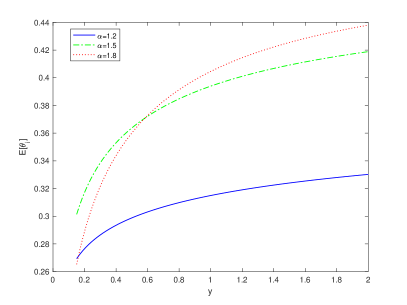
Figure 4: The expected number of clusters (left) and the duration of one cluster (right) as a function of the jump threshold $y$, for different values of $\alpha$.

When the jump threshold $y$ becomes extremely large, the point process $\{J_{t}^{(y)}\}$ is asymptotic to a Poisson process and the expected number of clusters converges to a fixed level, as shown by the following result.

Proposition 5.4

Let $\{y_{n}\}_{n\geq 1}$ be the sequence of positive thresholds with $y_{n}\sim cn^{1/\alpha}$ as $n\rightarrow\infty$ where $c$ is some positive constant. Then for each $t\geq 0$,

$$J^{(y_{n})}_{nt}\overset{w}{\longrightarrow}J_{t},$$ (46)

as $n\rightarrow\infty$, where $J$ is a Poisson process with the parameter $\lambda$ given by

$$\lambda=-\frac{\sigma_{N}^{\alpha}b}{\alpha\cos(\pi\alpha/2)\Gamma(-\alpha)c^{\alpha}},\quad 1<\alpha<2.$$

6 Appendix

Proof of Proposition 3.2. As a a direct consequence of [13] and [33], the proof mainly serves to provide the explicit form of the generalized Riccati equations. By (1) we have

$$dY_{t}=(r-\frac{1}{2}V_{t})dt+\rho\int_{0}^{V_{t}}W(dt,du)+\sqrt{1-\rho^{2}}\int_{0}^{V_{t}}\overline{W}(dt,du).$$

By Ito’s formula, we have that the process $(Y_{t},V_{t},\int_{0}^{t}V_{s}ds)$ is an affine process with generator given by

$$Af(y,v,u) = (r-\frac{1}{2}v)f^{\prime}_{y}(y,v,u)+a(b-v)f^{\prime}_{v}(y,v,u)+vf^{\prime}_{u}(y,v,u)$$

$$+\frac{1}{2}vf^{\prime\prime}_{yy}(y,v,u)+\rho\sigma vf^{\prime\prime}_{yv}(y,v,u)+\frac{1}{2}\sigma^{2}vf^{\prime\prime}_{vv}(y,v,u)$$

$$+\sigma_{N}^{\alpha}v\int_{0}^{\infty}\big{(}f(y,v+\zeta,u)-f(y,v,u)-f^{\prime}_{v}(y,v,u)\zeta\big{)}\nu_{\alpha}(d\zeta).$$

Denote by $X_{t}=(Y_{t},V_{t},\int_{0}^{t}V_{s}ds)$. We aim to find some functions $(\phi,\tilde{\Psi})\in\mathbb{C}\times\mathbb{C}^{3}$ with $\phi(0,\xi)=0$ and $\tilde{\Psi}(0,\xi)=\xi$ such that the following duality holds

$${\mathbb{E}}\left[e^{\langle\xi,X_{T}\rangle}\right]=\exp\Big{(}\phi(T,\xi)+\langle\tilde{\Psi}(T,\xi),X_{0}\rangle\Big{)}.$$ (47)

In fact, if

$$M_{t}=f(t,X_{t})=\exp\Big{(}\phi(T-t,\xi)+\langle\tilde{\Psi}(T-t,\xi),X_{t}\rangle\Big{)}$$

is a martingale, then we immediately have that

$$\mathbb{E}[e^{\langle\xi,X_{T}\rangle}]=\mathbb{E}[M_{T}]=M_{0}=\exp\Big{(}\phi(T,\xi)+\langle\tilde{\Psi}(T,\xi),X_{0}\rangle\Big{)},$$

which implies (47). Now assume that $(\phi,\tilde{\Psi})$ are sufficiently differential and applying the Ito formula to $f(t,X_{t})$, we have that

$$M_{T}-M_{0} = \mbox{local martingale part}-\int_{0}^{T}f(t,X_{t})\Big{(}\dot{\phi}(T-t,\xi)+\langle X_{t},\dot{\tilde{\Psi}}(T-t,\xi)\rangle\Big{)}dt$$

$$+\int_{0}^{T}f(t,X_{t})\tilde{\Psi}_{1}(T-t,\xi)(r-\frac{1}{2}V_{t})dt+\int_{0}^{T}f(t,X_{t})\tilde{\Psi}_{2}(T-t,\xi)a(b-V_{t})dt$$

$$+\int_{0}^{T}f(t,X_{t})\tilde{\Psi}_{3}(T-t,\xi)V_{t}dt+\frac{1}{2}\int_{0}^{T}f(t,X_{t})\tilde{\Psi}^{2}_{1}(T-t,\xi)V_{t}dt$$

$$+\rho\sigma\int_{0}^{T}f(t,X_{t})\tilde{\Psi}_{1}(T-t,\xi)\tilde{\Psi}_{2}(T-t,\xi)V_{t}dt+\frac{1}{2}\sigma^{2}\int_{0}^{T}f(t,X_{t})\tilde{\Psi}_{2}^{2}(T-t,\xi)V_{t}dt$$

$$+\sigma_{N}^{\alpha}\int_{0}^{T}f(t,X_{t})V_{t}\int_{0}^{\infty}\Big{[}\exp\{\tilde{\Psi}_{2}(T-t,\xi)z\}-1-\tilde{\Psi}_{2}(T-t,\xi)z\Big{]}\nu_{\alpha}(dz)$$

where $\tilde{\Psi}=(\tilde{\Psi}_{1},\tilde{\Psi}_{2},\tilde{\Psi}_{3})$. Then $f(t,X_{t})$ is a local martingale, if

$$\dot{\phi}(T-t,\xi)=r\tilde{\Psi}_{1}(T-t,\xi)+ab\tilde{\Psi}_{2}(T-t,\xi),\quad\dot{\tilde{\Psi}}_{1}(T-t,\xi)=0,\quad\dot{\tilde{\Psi}}_{3}(T-t,\xi)=0,$$

and

$$\dot{\tilde{\Psi}}_{2}(T-t,\xi) = -\frac{1}{2}\tilde{\Psi}_{1}(T-t,\xi)-a\tilde{\Psi}_{2}(T-t,\xi)+\tilde{\Psi}_{3}(T-t,\xi)$$

$$+\frac{1}{2}\tilde{\Psi}_{1}^{2}(T-t,\xi)+\rho\sigma\tilde{\Psi}_{1}(T-t,\xi)\tilde{\Psi}_{2}(T-t,\xi)+\frac{1}{2}\sigma^{2}\tilde{\Psi}^{2}_{2}(T-t,\xi)$$

$$+\sigma_{N}^{\alpha}\int_{0}^{\infty}\Big{(}e^{z\tilde{\Psi}_{2}(T-t,\xi)}-1-z\tilde{\Psi}_{2}(T-t,\xi))\Big{)}\nu_{\alpha}(dz).$$

Then we have that $\tilde{\Psi}_{1}(t,\xi)=\xi_{1}$ and $\tilde{\Psi}_{3}(t,\xi)=\xi_{3}$ for $0\leq t\leq T$. Furthermore $\tilde{\Psi}_{2}(t,\xi)$ solves the ODE

$$\dot{\tilde{\Psi}}_{2}(t,\xi) = -\frac{1}{2}\xi_{1}-a\tilde{\Psi}_{2}(t,\xi)+\xi_{3}+\frac{1}{2}\xi_{1}^{2}+\rho\sigma\xi_{1}\tilde{\Psi}_{2}(t,\xi)+\frac{1}{2}\sigma^{2}\tilde{\Psi}^{2}_{2}(t,\xi)$$

$$+\sigma_{N}^{\alpha}\int_{0}^{\infty}\Big{(}e^{z\tilde{\Psi}_{2}(t,\xi)}-1-z\tilde{\Psi}_{2}(t,\xi))\Big{)}\nu_{\alpha}(dz)$$

$$= -\frac{1}{2}\xi_{1}-a\tilde{\Psi}_{2}(t,\xi)+\xi_{3}+\frac{1}{2}\xi_{1}^{2}+\rho\sigma\xi_{1}\tilde{\Psi}_{2}(t,\xi)+\frac{1}{2}\sigma^{2}\tilde{\Psi}^{2}_{2}(t,\xi)-\frac{\sigma_{N}^{\alpha}}{\cos(\pi\alpha/2)}(-\tilde{\Psi}_{2}(t,\xi))^{\alpha}$$

Now let $\Psi(t,\xi)=\tilde{\Psi}_{2}(t,\xi)$, which obviously satisfies the ODE (9) and

$$\phi(t,\xi)=\int_{0}^{t}(r\xi_{1}+ab\Psi(s,\xi)ds.$$

The proof is thus complete. $\Box$

Proof of Lemma 4.3. Consider (24). By Doob’s inequality,

$$\mathbb{E}_{x}\Big{[}\sup_{0\leq t\leq T}\Big{|}\int_{0}^{t}e^{-a(t-s)}\sqrt{V_{s}}dB_{s}\Big{|}^{2}\Big{]}\leq 4\mathbb{E}_{x}\Big{[}\int_{0}^{T}e^{2as}V_{s}ds\Big{]}\leq\frac{2x+b}{2a}e^{2aT}，$$

which implies that $u^{\alpha}\mathbb{P}_{x}(\sup_{0\leq t\leq T}|\int_{0}^{t}e^{-a(t-s)}\sqrt{V_{s}}dB_{s}|>u)\rightarrow 0$ as $u\rightarrow\infty$. Then, in view of (24), the extremal behavior of $V_{t}$ in the sense of (16) is determined by

$$\sigma_{N}\int_{0}^{t}e^{-a(t-s)}\sqrt[\alpha]{V_{s-}}dZ_{s}=e^{-at}\cdot\sigma_{N}\int_{0}^{t}e^{as}\sqrt[\alpha]{V_{s-}}dZ_{s}:=X_{t}\cdot Y_{t}.$$

Note that $\mathbb{E}[\sup_{0\leq t\leq T}(\sqrt[\alpha]{V_{t}})^{\alpha+\delta}]<\infty$ for $0<\delta<\alpha(\alpha-1)$ from Lemma 4.7. Then by [28, Theorem 3.4], we have as $u\rightarrow\infty$,

$$u^{\alpha}\mathbb{P}({Y}/u\in\cdot)\overset{\widehat{w}}{\longrightarrow}\delta_{Y}(\cdot)\quad on\quad\mathscr{B}(\bar{D}_{0}([0,T]),$$ (48)

where $\delta$ is given by:

$$\delta_{Y}(\cdot)=T\mathbb{E}\Big{[}\int_{0}^{\infty}1_{\{w_{t}:=\sigma_{N}e^{a\tau}\sqrt[\alpha]{V_{\tau}}y1_{[\tau,T]}(t)\in\cdot\}}\nu_{\alpha}(dy)\Big{]},$$

where $\tau$ is uniformly distributed on $[0,T]$ and independent of $V$. Furthermore, by [28, Theorem 3.1], we have as $u\rightarrow\infty$,

$$u^{\alpha}\mathbb{P}({XY}/u\in\cdot)\overset{\widehat{w}}{\longrightarrow}\delta_{Y}(w\in\bar{D}_{0}[0,T]:Xw\in\cdot)\quad on\quad\mathscr{B}(\bar{D}_{0}([0,T]),$$

A simple calculation shows that

$$\delta(\cdot):=\delta_{Y}(w\in\bar{D}_{0}[0,T]:Xw\in\cdot)=\sigma_{N}^{\alpha}\int_{0}^{T}\mathbb{E}[V_{s}]\int_{0}^{\infty}1_{\{w_{t}=e^{-a(t-s)}y1_{[s,T]}(t)\in\cdot\}}\nu_{\alpha}(dy)ds$$

$\Box$

Proof of Lemma 4.7. By (24), an elementary inequality shows that there exists a locally bounded function $C_{1}(\cdot)$ such that

$$\mathbb{E}_{x}\Big{[}\sup_{0\leq t\leq T}V_{t}^{\beta}\Big{]} \leq C_{1}(T)\Big{(}x^{\beta}+b^{\beta}+\sigma^{\beta}\mathbb{E}_{x}\Big{[}\sup_{0\leq t\leq T}\big{|}\int_{0}^{t}e^{-a(t-s)}\sqrt{V_{s}}dB_{s}\big{|}^{\beta}\Big{]}$$ (49)

$$+\sigma^{\beta}_{N}\mathbb{E}_{x}\Big{[}\sup_{0\leq t\leq T}\big{|}\int_{0}^{t}e^{-a(t-s)}V_{s-}^{1/\alpha}dZ_{s}\big{|}^{\beta}\Big{]}\Big{)}.$$

By Hölder’s inequality and Doob’s martingale inequality, there exist a locally bounded function $C_{2}(\cdot)$ such that

$$\begin{split}&\quad\mathbb{E}_{x}\Big{[}\sup_{0\leq t\leq T}\Big{|}\int_{0}^{t}e^{-a(t-s)}\sqrt{V_{s}}dB_{s}\Big{|}^{\beta}\Big{]}\leq 2^{\beta}\mathbb{E}_{x}\Big{[}\Big{(}\int_{0}^{T}e^{2as}V_{s}ds\Big{)}^{\beta/2}\Big{]}\\ &\leq 2^{\beta}\Big{(}\int_{0}^{T}\mathbb{E}_{x}[e^{2as}V_{s}]ds\Big{)}^{\beta/2}\leq C_{2}(T)\left(x^{\beta/2}e^{\beta aT/2}+e^{\beta aT}\right).\end{split}$$

Moreover, by Long [38, Lemma 2.4], which is a generalization of Rosinski and Woyczynski [41, Theorem 3.2], there exist locally bounded functions $C_{3}(\cdot)$ and $C_{4}(\cdot)$ such that

$$\begin{split}&\quad\mathbb{E}_{x}\Big{[}\sup_{0\leq t\leq T}\Big{|}\int_{0}^{t}e^{-a(t-s)}V_{s-}^{1/\alpha}dZ_{s}\Big{|}^{\beta}\Big{]}\leq C_{3}(T)\mathbb{E}_{x}\Big{[}\Big{(}\int_{0}^{T}e^{\alpha as}V_{s}ds\Big{)}^{\beta/\alpha}\Big{]}\\ &\leq C_{3}(T)\Big{(}\int_{0}^{T}\mathbb{E}_{x}[e^{\alpha as}V_{s}]ds\Big{)}^{\beta/\alpha}\leq C_{4}(T)\left(x^{\beta/\alpha}e^{\beta a(1-1/\alpha)T}+e^{\beta aT}\right).\end{split}$$

By combining (49), (6) and (6), we have the lemma. $\Box$

Proof of Lemma 5.1. By (2), we note that

$$\{\tau_{1}>t\}=\Big{\{}\tau_{1}>t,\ \int_{0}^{t}\int_{0}^{V_{s-}}\int_{\overline{y}}^{\infty}\zeta N(ds,du,d\zeta)=0\Big{\}}.$$

Since $V^{(y)}$ coincides with $V$ up to $\tau_{1}$, the comparison between (2) and (35) implies that

$$\{\tau_{1}>t\}=\Big{\{}\tau_{1}>t,\ \int_{0}^{t}\int_{0}^{V^{(y)}_{s-}}\int_{\overline{y}}^{\infty}\zeta N(ds,du,d\zeta)=0\Big{\}}\;a.s.$$

If $\tau_{1}\leq t$, we immediately have

$$\int_{0}^{t}\int_{0}^{V^{(y)}_{s-}}\int_{\overline{y}}^{\infty}\zeta N(ds,du,d\zeta) \geq \int_{0}^{\tau_{1}}\int_{0}^{V^{(y)}_{s-}}\int_{\overline{y}}^{\infty}\zeta N(ds,du,d\zeta)$$

$$= \int_{0}^{\tau_{1}}\int_{0}^{V_{s-}}\int_{\overline{y}}^{\infty}\zeta N(ds,du,d\zeta)>0.$$

Thus

$$\{\tau_{1}>t\}=\Big{\{}\int_{0}^{t}\int_{0}^{V^{(y)}_{s-}}\int_{\overline{y}}^{\infty}\zeta N(ds,du,d\zeta)=0\Big{\}}\;a.s.$$ (50)

Recall that $1_{\{\zeta>\overline{y}\}}N(ds,du,d\zeta)$ is the restriction of $N(ds,du,d\zeta)$ to $(0,\infty)\times(0,\infty)\times(\overline{y},\infty)$, which is independent of $1_{\{\zeta\leq\overline{y}\}}N(ds,du,d\zeta)$. By (35) we have that $1_{\{\zeta>\overline{y}\}}N(ds,du,d\zeta)$ is independent of $(V^{(y)}_{t},t\geq 0)$. Then conditional on $(V^{(y)}_{t},t\geq 0)$, $\int_{0}^{t}\int_{0}^{V^{(y)}_{s-}}\int_{\overline{y}}^{\infty}{N}(ds,du,d\zeta)$ is a time inhomogenous Poisson process with intensity function $\big{(}\int_{\overline{y}}^{\infty}\nu_{\alpha}(d\zeta)\big{)}V^{(y)}_{.}$. Note that $\tau_{1}$ is the first jump time of $\sigma_{Z}\int_{0}^{t}\int_{0}^{V^{(y)}_{s-}}\int_{\overline{y}}^{\infty}{N}(ds,du,d\zeta)$, and $\Delta V_{\tau_{1}}$ is the first jump size of $\sigma_{Z}\int_{0}^{t}\int_{0}^{V^{(y)}_{s-}}\int_{\overline{y}}^{\infty}{N}(ds,du,d\zeta)$. Then we have

$$\mathbb{E}\big{[}\tau_{1}\in dt,\ \Delta V_{\tau_{1}}\in d\zeta\,|V_{.}^{(y)}\big{]}=\Big{(}\int_{\overline{y}}^{\infty}\nu_{\alpha}(dx)\Big{)}\,\Big{(}V^{(y)}_{t}dt\Big{)}\,\Big{(}\frac{\alpha y^{\alpha}1_{\{\zeta>y\}}}{\zeta^{1+\alpha}}d\zeta\Big{)},$$

which implies that $\Delta V_{\tau_{1}}$ is independent of $\tau_{1}$ and $V^{(y)}$. $\Box$

Proof of Propositon 5.2

Step 1. Recall that $\tau_{1}=\inf\{t>0:\Delta V_{t}>y\}$ and $T_{1}$ is the first jump time of the point process $\{J_{t}:t\geq 0\}$ given by (39). By (50), we immediately get $\tau_{1}=T_{1}$ a.s.. Thus by Lemma 5.1, we have that $V^{(y)}$ coincides with $V$ up to $T_{1}$ and $\Delta V_{T_{1}}$ is independent of $V^{(y)}$. Note that $V^{(y)}_{T_{1}}=V_{T_{1}-}$ and

$$\begin{split}{V}^{(y)}_{t}=V_{T_{1}-}&+\int_{T_{1}}^{t}\widetilde{a}(\alpha,y)\big{(}\widetilde{b}(\alpha,y)-{V}_{s}^{(y)}\big{)}ds+\sigma\int_{T_{1}}^{t}\int_{0}^{{V}_{s}^{(y)}}W(ds,du)\\ &+\sigma_{N}\int_{T_{1}}^{t}\int_{0}^{{V}_{s-}^{(y)}}\int_{0}^{\overline{y}}\zeta\widetilde{N}(ds,du,d\zeta),\quad t\geq T_{1}.\end{split}$$ (51)

By taking $k=1$ in (40),

$$\begin{split}v_{t}^{(1)}=\Delta V_{T_{1}}&-a\int_{T_{1}}^{t}v^{(1)}_{s}ds+\sigma\int_{T_{1}}^{t}\int_{{V}^{(y)}_{s}}^{{V}^{(y)}_{s}+v^{(1)}_{s}}W(ds,du)\\ &+\sigma_{N}\int_{T_{1}}^{t}\int_{{V}^{(y)}_{s-}}^{{V}^{(y)}_{s-}+v^{(1)}_{s-}}\int_{\mathbb{R}^{+}}\zeta\widetilde{N}(ds,du,d\zeta),\quad t\geq T_{1}.\end{split}$$ (52)

As mentioned above, $\Delta_{T_{1}}$ is independent of $V_{T_{1}-}$. By using the property of independent and stationary increments of $W$ and $N$, we have that $v^{(1)}$ and $V^{(y)}$ are independent of each other and $\{u^{(1)}_{t}:=v^{(1)}_{T_{1}+t},\ t\geq 0\}$ is a CB process which has the same distribution as $u$ given by (42); see e.g., [12, Theorem 3.2, 3.3]). Now set

$$\begin{split}\bar{V}_{t}^{(1)}=V_{T_{1}-}&+\int_{T_{1}}^{t}a\left(b-\bar{V}_{s}^{(1)}\right)ds+\sigma\int_{T_{1}}^{t}\int_{0}^{\bar{V}_{s}^{(1)}}W(ds,du)\\ &+\sigma_{N}\int_{T_{1}}^{t}\int_{0}^{\bar{V}_{s-}^{(1)}}\int_{\mathbb{R}^{+}}\zeta\widetilde{N}(ds,du,d\zeta),\quad t\geq T_{1}.\end{split}$$ (53)

It is easy to see $\bar{V}^{(1)}$ is of the same type as $V$ but with initial value $V_{T_{1}-}$ and starting from time $T_{1}$. Define

$$\bar{\tau}_{1}:=\inf\{t>T_{1}:\Delta\bar{V}_{t}^{(1)}>y\},$$

which is the first jump time of $\bar{V}^{(1)}$ whose jump size larger than $y$. Then a comparison of (51) and (56) shows that $\bar{V}^{(1)}_{t}=V_{t}^{(y)}$ for $t\in[T_{1},\bar{\tau}_{1})$. Furthermore the similar proof of Lemma 5.1 shows that for any $t>0$,

$$\{\bar{\tau}_{1}-T_{1}>t\}=\Big{\{}\int_{T_{1}}^{T_{1}+t}\int_{0}^{V^{(y)}_{s-}}\int_{\overline{y}}^{\infty}\zeta N(ds,du,d\zeta)=0\Big{\}}\;a.s.,$$

which implies that $\bar{\tau}_{1}=T_{2}$ a.s. Thus $\Delta\bar{V}^{(1)}_{\bar{\tau}_{1}}=\Delta V_{T_{2}}$ and $\Delta V_{T_{2}}$ is independent of $V^{(y)}$ and $\Delta V_{T_{1}}$. Furthermore $\bar{V}^{(1)}_{t}=V_{t}^{(y)}$ for $t\in[T_{1},T_{2})$. We get that

$$V^{(y)}_{t}+v^{(1)}_{t}=\bar{V}_{t}^{(1)}+v^{(1)}_{t}=V_{t},\ a.s.\quad t\in[T_{1},T_{2}).$$ (54)

The third equality follows from (56), (52) and (2).

Step 2. By taking $k=2$ in (40),

$$\begin{split}v_{t}^{(2)}=\Delta V_{T_{2}}&-a\int_{T_{2}}^{t}v^{(2)}_{s}ds+\sigma\int_{T_{2}}^{t}\int_{{V}^{(y)}_{s}+v^{(1)}_{s}}^{{V}^{(y)}_{s}+v^{(1)}_{s}+v^{(2)}_{s}}W(ds,du)\\ &+\sigma_{N}\int_{T_{2}}^{t}\int_{{V}^{(y)}_{s-}+v^{(1)}_{s-}}^{{V}^{(y)}_{s-}+v^{(1)}_{s-}+v^{(2)}_{s-}}\int_{\mathbb{R}^{+}}\zeta\widetilde{N}(ds,du,d\zeta),\quad t\geq T_{2}.\end{split}$$ (55)

Since $\Delta V_{T_{2}}$ is independent of $V^{(y)}_{T_{2}}$ and $\Delta V_{T_{1}}$, still by using the property of independent and stationary increments of $W$ and $N$, we have that $v^{(2)}$ are independent of $V^{(y)}$ and $v^{(1)}$, and $\{u^{(2)}_{t}:=v^{(2)}_{T_{2}+t},\ t\geq 0\}$ is also a CB process which has the same distribution as $u$. Now set

$$\begin{split}\bar{V}_{t}^{(2)}=V^{(y)}_{T_{2}}&+\int_{T_{2}}^{t}a\left(b-\bar{V}_{s}^{(2)}\right)ds+\sigma\int_{T_{2}}^{t}\int_{0}^{\bar{V}_{s}^{(2)}}W(ds,du)\\ &+\sigma_{N}\int_{T_{2}}^{t}\int_{0}^{\bar{V}_{s-}^{(2)}}\int_{\mathbb{R}^{+}}\zeta\widetilde{N}(ds,du,d\zeta),\quad t\geq T_{2}.\end{split}$$ (56)

Define

$$\bar{\tau}_{2}:=\inf\{t>T_{2}:\Delta\bar{V}_{t}^{(2)}>y\},$$

As proved in Step 2 we have that $\bar{\tau}_{2}=T_{3}$ a.s. and $\bar{V}^{(2)}_{t}=V_{t}^{(y)}$ for $t\in[T_{2},T_{3})$. Note that $V_{T_{2}-}=V^{(y)}_{T_{2}}+\Delta r^{(1)}_{T_{2}}$ by (54). We get that

$$V^{(y)}_{t}+v^{(1)}_{t}+v^{(2)}=\bar{V}_{t}^{(2)}+v^{(1)}_{t}+v^{(2)}_{t}=V_{t},\ a.s.\quad t\in[T_{2},T_{3}).$$

Step 3. By induction, it is not hard to prove that $V_{t}=V^{(y)}_{t}+\sum_{k=1}^{n}v^{(k)}_{t}$ holds for any $t\in[T_{n},T_{n+1})$ and $n\geq 1$, and the sequence of i.i.d processes is of the same distribution as $u$. Furthermore $\{u^{(n)}\}$ is independent of $V^{(y)}$. Then we have this proposition. $\Box$

Proof of Propositon 5.3  (1) Note that $J_{t}^{(y)}\overset{d}{=}\int_{0}^{t}\int_{0}^{V_{s-}^{(y)}}\int_{D}M(ds,du,d\omega)$. Then

$$\mathbb{E}[J_{t}^{(y)}]=\int_{0}^{t}\mathbb{E}[V_{s}^{(y)}]ds\int_{\bar{y}}^{\infty}\nu_{\alpha}(d\zeta).$$

A simple computation shows (43). (2) By Proposition 5.2, $u^{(n)}$ is a subcritical CB process without immigration, i.e. the branching mechanism is

$$\Psi_{\alpha}(q)=aq+\frac{\sigma^{2}}{2}q^{2}-\frac{\sigma_{N}^{\alpha}}{\cos(\pi\alpha/2)}q^{\alpha}.$$

and the immigration rate $\Phi(q)=0$. Then $0$ is an absorbing point of $\theta_{n}$ and $\theta_{n}$ is the extinct time of CB process $u^{(n)}$. Since $\int_{1}^{\infty}1/\Psi_{\alpha}(u)du<\infty$, the so-called Grey’s condition is satisfied, it follows from Grey [24, Theorem 1] that

$$\mathbb{P}(\theta_{n}<\infty)=\int_{0}^{\infty}\mathbb{P}_{x}(\theta_{n}<\infty)\mathbb{P}(\Delta V_{T_{n}}\in dx)=1.$$

Furthermore, still by [24, Theorem 1], we have that

$$\mathbb{P}(\theta_{n}>t)=\mathbb{E}[1-e^{-{\Delta V_{T_{n}}q_{t}}}]=\alpha y^{\alpha}\int_{y}^{\infty}(1-e^{-xq_{t}})x^{-(1+\alpha)}dx,$$ (57)

where $q_{t}$ is the minimal solution of the ODE

$$\frac{d}{dt}q_{t}=-\Psi_{\alpha}(q_{t}),\quad t>0,$$

with $q_{0+}=\infty$. In this case, $0<q_{t}<\infty$ for $t\in(0,\infty)$. Then

$$\mathbb{E}[\theta_{n}]=\alpha y^{\alpha}\int_{0}^{\infty}\int_{y}^{\infty}(1-e^{-xq_{s}})x^{-(1+\alpha)}dxds,$$

which gives (44) by (57). $\Box$

Proof of Propositon 5.4 By (39), we have

$$J_{nt}^{(y_{n})}=\int_{0}^{nt}\int_{0}^{V^{(y_{n})}_{s-}}\int_{\bar{y}_{n}}^{\infty}N(ds,du,d\zeta)$$

where $\bar{y}_{n}=y_{n}/\sigma_{N}$. It follows from Proposition 5.2-(2) that for any $\theta>0$,

$$\mathbb{E}\Big{[}e^{-\theta J_{nt}^{(y_{n})}}\Big{]} = \mathbb{E}\bigg{[}\exp\bigg{\{}\Big{(}\int_{\bar{y}_{n}}^{\infty}\nu_{\alpha}(d\xi)\Big{)}\int_{0}^{nt}V_{s}^{(y_{n})}ds\Big{(}e^{-\theta}-1\Big{)}\bigg{\}}\bigg{]}$$ (58)

$$= \mathbb{E}\bigg{[}\exp\bigg{\{}\Big{(}n\int_{\bar{y}_{n}}^{\infty}\nu_{\alpha}(d\xi)\Big{)}\frac{1}{n}\int_{0}^{nt}V_{s}^{(y_{n})}ds\Big{(}e^{-\theta}-1\Big{)}\bigg{\}}\bigg{]}.$$

Based on (35), for fixed $y_{n}$, $\{V_{t}^{(y_{n})}:t\geq 0\}$ is a CBI process. By [30, Remark 5.3], for $\theta>0$,

$$\mathbb{E}\bigg{[}e^{-\frac{\theta}{n}\int_{0}^{nt}V_{s}^{(y_{n})}ds}\bigg{]}=\exp\bigg{\{}-v_{n}(\theta,nt)V_{0}-ab\int_{0}^{nt}v_{n}(\theta,s)ds\bigg{\}}$$ (59)

where $v_{n}(\theta,t)$ is the unique solution of

$$\frac{dv_{n}(\theta,t)}{dt}=\frac{\theta}{n}-\Psi_{n}(v_{n}(\theta,t)),$$ (60)

with $v_{n}(\theta,0)=0$, and

$$\Psi_{n}(q)=\Big{(}a+\sigma_{N}^{\alpha}\int_{y_{n}}^{\infty}\xi\nu_{\alpha}(d\xi)\Big{)}q+\frac{\sigma^{2}}{2}q^{2}+\sigma_{N}^{\alpha}\int_{0}^{y_{n}}(e^{-q\xi}-1+q\xi)\nu_{\alpha}(d\xi).$$

Then we have $-\Psi_{n}(v_{n}(\theta,t))\leq\frac{dv_{n}(\theta,t)}{dt}\leq\frac{\theta}{n}-av_{n}(\theta,t)$, which implies that $0\leq v_{n}(\theta,t)\leq\frac{\theta}{an}(1-e^{-at})$. By (60),

$$nv_{n}(\theta,nt)=\frac{\theta}{a_{n}}(1-e^{-na_{n}t})-\int_{0}^{nt}e^{-a_{n}(nt-s)}n\widehat{\Psi}_{n}(v_{n}(\theta,s))ds,$$ (61)

where

$$a_{n}=a+\sigma_{N}^{\alpha}\int_{y_{n}}^{\infty}\xi\nu_{\alpha}(d\xi),\quad\widehat{\Psi}_{n}(q)=\frac{\sigma^{2}}{2}q^{2}+\sigma_{N}^{\alpha}\int_{0}^{y_{n}}(e^{-q\xi}-1+q\xi)\nu_{\alpha}(d\xi).$$

Note that $a_{n}\rightarrow a$, and for all $t\geq 0$ and $n\geq 1$,

$$0\leq nv_{n}(\theta,t)\leq\frac{\theta}{a},\quad n\widehat{\Psi}_{n}(v_{n}(\theta,t))\leq\frac{\sigma^{2}\theta^{2}}{2a^{2}n}-\frac{\sigma_{N}^{\alpha}\theta^{\alpha}}{\cos(\pi\alpha/2)a^{\alpha}n^{\alpha-1}}.$$

By (61), we have $nv_{n}(\theta,nt)\rightarrow\frac{\theta}{a}$ and then

$$\int_{0}^{nt}v_{n}(\theta,s)ds=\int_{0}^{t}nv_{n}(\theta,ns)ds\rightarrow\frac{\theta t}{a}.$$

Thus by (59), we have for any $t\geq 0$,

$$\frac{\int_{0}^{nt}V_{s}^{(y_{n})}ds}{n}\overset{p}{\rightarrow}bt.$$

Recall that $y_{n}\sim cn^{1/\alpha}$. Then $n\int_{\bar{y}_{n}}^{\infty}\nu_{\alpha}(d\xi)\rightarrow-\frac{\sigma_{N}^{\alpha}}{\alpha\cos(\pi\alpha/2)\Gamma(-\alpha)c^{\alpha}}$. By (58),

$$\mathbb{E}\Big{[}e^{-\theta J_{nt}^{(y_{n})}}\Big{]}\rightarrow\exp\bigg{\{}-\frac{\sigma_{N}^{\alpha}bt}{\alpha\cos(\pi\alpha/2)\Gamma(-\alpha)c^{\alpha}}(e^{-\theta}-1)\bigg{\}}.$$

We are done.

References

• [1] Abi Jaber, E., Larsson, M. and Pulido, S. (2017): Affine Volterra processes. Working Paper
• [2] Avellaneda, M. and Papanicolaou, A. (2018): Statistics of VIX Futures and Applications to Trading Volatility Exchange-Traded Products. Journal of Investment Strategies, 7(2), 1-33.
• [3] Asmussen, S. and Rosinski, J.: Approximations of small jumps of Lévy processes with a view towards simulation, Journal of Applied Probability, 38, 482-493 (2001).
• [4] Barndorff-Nielsen, E. and Shephard, N. (2001): Non-Gaussian Ornstein-Uhlenbeck-based models and some of their uses in financial economics, Journal of Royal Statistical Society, Series B, 63(2), 167-241.
• [5] Bates, D. (1996): Jump and stochastic volatility: exchange rate processes implicit in Deutsche market options, Review of Financial Studies, 9, 69-107.
• [6] Bayer, C.; Friz, P., and Gatheral, J. (2016): Pricing under rough volatility. Quantitative Finance, 16(6), 887-904.
• [7] Bingham, N. H., Goldie C. M. and Teugels, J. L. (1987): Regular Variation. Cambridge: Cambridge Univ Press.
• [8] Bingham, N. H. and Teugels, J. L. (1975): Duality for regularly varying functions. Quart J Math Oxford, 26, 333-353.
• [9] Carr, P. and Lee, R. (2007): Realized volatility and variance: options via swaps, RISK, 20, 76-83.
• [10] Cox, J., Ingersoll, J. and Ross, S.: A theory of the term structure of interest rate. Econometrica, 53, 385-408 (1985).
• [11] Da Fonseca, J. and Grasselli, M. (2011): Riding on the smiles. Quantitative Finance 11.11 (2011): 1609-1632.
• [12] Dawson, A and Li, Z.: Stochastic equations, flows and measure-valued processes. Annals of Probability, 40(2), 813-857 (2012).
• [13] Duffie, D., Pan, J. and Singleton, K. (2000): Transform analysis and asset pricing for affine jump-diffusions. Econometrica, 68(6), 1343-1376.
• [14] Duffie, D., Filipović, D. and Schachermayer, W.: Affine processes and applications in finance, Annals of Applied Probability, 13(3), 984-1053 (2003).
• [15] Duquesne, T. and Labbé, C. (2014): On the Eve property for CSBP, Electron. J. Probab. 19, no. 6, 31 pages.
• [16] El Euch, O. and Rosenbaum M. (2016): The characteristic function of rough Heston model, preprint to appear in Mathematical Finance.
• [17] El Euch, O., Fukasawa, M. and Rosenbaum M. (2016) The microstructural foundations of leverage effect and rough volatility, preprint to appear in Finance and Stochastics.
• [18] Errais, E., Giesecke, K., Goldberg, L. (2010): Affine point processes and portfolio credit risk. SIAM Journal on Financial Mathematics, 1, 642-665.
• [19] Filipović, D. (2001): A general characterization of one factor affine term structure models, Finance and Stochastics, 5(3), 389-412.
• [20] Fu, Z. and Li, Z. (2010): Stochastic equations of non-negative processes with jumps. Stochastic Processes and their Applications, 120, 306-330.
• [21] Gatheral, J., Jaisson, T. and Rosenbaum, M. (2014): Volatility is rough. Preprint to appear in Quantitative Finance, arXiv:1410.3394.
• [22] Goard, J., and Mazur, M. (2013). Stochastic volatility models and the pricing of VIX options. Mathematical Finance, 23(3), 439-458.
• [23] Grasselli, M. (2016). The 4/2 stochastic volatility model: a unified approach for the Heston and the 3/2 model. Mathematical Finance.
• [24] Grey, D.R. (1974): Asymptotic behavior of continuous time continuous state-space branching processes. J. Appl. Prob. 11, 669-677.
• [25] Gulisashvili, A. (2010): Asmptotic formulas with error estimates for call pricing functions and the implied volatility at extreme strikes. Siam J. Financial Math. 1,609-641.
• [26] Hawkes, A. G. (1971): Spectra of Some Self-Exciting and Mutually Exciting Point Processes. Biometrika, 58, 83-90.
• [27] Heston, S. (1993): A closed form solution for options with stochastic volatility with applications to bond and currency options, Review of Financial Studies 6, 2, 327-344.
• [28] Hult, H. and Lindskog, F. (2007): Extremal behavior of stochastic integrals driven by regularly Lévy processes.Ann. Probab. 35, 309-339.
• [29] Jaisson, T., and Rosenbaum, M. (2015): Limit theorems for nearly unstable Hawkes processes. Annals of Applied Probability, 25(2), 600-631.
• [30] Jiao, Y., Ma, C. and Scotti S. (2017): Alpha-CIR model with branching processes in sovereign interest rate modeling, Finance and Stochastics, 21(3), 789-813.
• [31] Kallsen, J. and Muhle-Karbe, J.: Exponentially affine martingales, affine measure changes and exponential moments of affine processes, Stochastic Processes and their Applications, 120, 163-181 (2010).
• [32] Kallsen, J., Muhle-Karbe, J. and Vo$\beta$, M. (2011): Pricing option on variance in affine stochastic volatility models, Mathematical Finance, 21, 627-641.
• [33] Keller-Ressel, M. (2011): Moment explosions and long-term behavior of affine stochastic volatility models. Mathematical Finance, 21, 73-98.
• [34] Lee, R. W.: The moment formula for implied volatility at extreme strikes. Mathematical Finance, 14(3), 469-480 (2004).
• [35] Li, Z.: Measure-Valued Branching Markov Processes, Springer, Berlin (2011).
• [36] Li, Z. and Ma, C.: Asymptotic properties of estimators in a stable Cox-Ingersoll-Ross model. Stochastic Processes and their Applications, 125(8), 3196-3233 (2015).
• [37] Liu, Y., Gopikrishnan, P., Cizeau, P., Meyer, M., Peng, C. K. and Stanley H.E. (1999): Statistical properties of the volatility of price fluctuations. Physical Review E, 60, 1390-1400.
• [38] Long, H. (2010): Parameter estimation for a class of stochastic differential equations driven by small stable noises from discrete observations. Acta Math. Sci. English Ed.30B, 645-663.
• [39] Nicolato, E. and Venardos, E. (2003): Option pricing in stochastic volatility models of the Ornstein-Uhlenbeck type, Mathematical Finance, 13 , 445-466.
• [40] Nicolato, E., Pisani, C. and Sloth, D. (2017): The impact of jump distributions on the implied volatility of variance, SIAM Journal on Financial Mathematics, 8, 28-53.
• [41] Rosinski, J. and Woyczynski, W.A. (1985): Moment inequalities for real and vector p-stable stochastic integrals. In: Probability in Banach Spaces V. Lecture Notes in Math. 1153, 369-386, Springer, Berlin.
• [42] Sepp, A. (2008): Pricing options on realized variance in the Heston model with jumps in returns and volatility, Journal of Computational Finance, 11, 33-70.