Influence of Demand and Generation Uncertainty on the Operational Efficiency of Smart Grids

Abstract

To ensure the smooth and near optimal operation of storage and controllable generation in a grid with a high share of renewable energies, it is important to have accurate forecasts for load and generation. But even with the advanced forecasts available today, the prediction error can have a significant impact on the operation performance of the system. This paper compares and analyzes the impact of the prediction-error on the operational performance in case of a small virtual power plant.

I Introduction

Governments around the world have made climate protection a priority policy goal. This is increasingly occurring as a result of climate change, and the environmental issues it has presented to us. To combat environmental degradation, a shift away from fossil fuels and towards renewable systems is required. In Germany for instance, renewable forms of energy are on the rise. In 1990, renewable energy sources accounted for just under 4% of total electrical energy production, but that share rose to as much as 33% by 2017 [1]. The number of consumers and producers who utilize renewable power generation systems has increased, which also entails new and increased challenges for system operators [2]. When the next generation shifts increasingly towards renewable resources, extensive planning is required to meet, as well as to coordinate and control the loads of individual consumers. This well informed policy will be crucial, as considerable uncertainties can interfere when planning for energy problems. Uncertainty from inaccurate projections of the future needs and capacities of renewable resources can also generate problems in micro grid operation. [3, 4, 5].

In this paper, the effects of the prediction error on the operational efficiency of a small self consumption community is investigated.

II Optimal Operation of Power Systems

The motivation to apply efficient resource scheduling in power systems has increased. It supports the economical and reliable energy production [6, 7]. It also determines the operation of generating resources. This minimizes the total generating cost while responding to the system boundaries as well as to the demands [8]. Dynamic programming [9], standard mixed integer programming as well as non-linear programming have been developed as solution methods to cope with scheduling problems in research areas. Further techniques encompass exact approaches such as Lagrange relaxation [10, 11], or heuristics and meta-heuristics methods [12, 13]. One of the most used approaches is the mixed-integer-linear programming (MILP) approach. Efficient solution techniques have been developed to guarantee convergence within few iterations [8, 6]. The production of large power systems is coordinated by these UC approaches. Therefore much effort has been made to optimize the problem formulation. This leads to a decreased number of binary variables which speeds up the process of search and limits the search space.

In this paper the underlying optimization problem is solved in a Model Predictive Control (MPC) fashion. Hereby a dynamic model of the energy system is used to predict the future behavior within a discrete time horizon $T$. This model depends on various inputs such as the predicted generation or demand. At each sample point the complete optimization problem is solved over the horizon but only the first step is implemented. The software has been implemented in python using CVXPY [14, 15]. An example of the optimized operation for a small self consumption community with renewable generation and a combined heat and power (CHP) cogeneration plant is shown in Fig. 1.

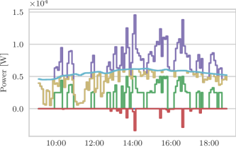
(a)

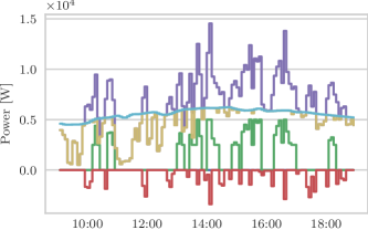
(b)

Figure 1: Exemplary results for the optimized operation. In Fig. 1a the relative prediction error is $0\text{\,}\mathrm{\char 37\relax}\text{/}$ and in Fig. 1b the relative prediction error is $10\text{\,}\mathrm{\char 37\relax}\text{/}$. The goal of the optimization in this case is to use as little energy from the grid as possible (negative feed in, red line).

III Problem Formulation

To standardize the modeling of renewable energy resources (PV, wind), intermittent generation units or energy storage devices with limited capacity, a standardized formulation according to the Power Node framework is used in this paper. The reader is referred to [16] for details. Depending on the device properties and the energy supply and demand the constraints are listed and the decision variables are defined to present the characteristic properties of power nodes. In the case of renewable energy generation plants, it is assumed that production can only be curtailed and that otherwise there is no possibility of influence. Consumers are assumed to be passive loads, i.e. not controllable. The cost function of the problem can be expressed as follows:

$$\underset{P_{g,t}}{\text{min}} \sum_{t\in T,g\in G} P_{g,t}\kappa_{g}$$ (1)

s.t. $$0 =\sum_{g\in G}P_{g,t},\quad t\in T$$

$$\dot{x}_{t} =C^{-1}p_{\text{batt}}$$

$$0 \leq x\leq 1$$

$$\underline{P}_{\text{batt}} \leq P_{\text{batt}}\leq\overline{P}_{\text{batt}}$$

$$0 \leq P_{\text{RES}}\leq\overline{P}_{\text{RES}}$$

$$\underline{P}_{\text{CHP}} \leq P_{\text{CHP}}\leq\overline{P}_{\text{CHP}}\quad\text{if}\;P_{\text{CHP}}>0$$

$$\underline{P}_{\text{grid}} \leq P_{\text{grid}}\leq\overline{P}_{\text{grid}}$$

hereby $P_{g}$ denotes power supply/demand by generator/consumer $g$ in the network, while the $\kappa_{g}$ regards to the price of per kWh supplied/consumed electricity [€ /kWh]. The variable $P_{\text{grid}}$ corresponds to the power delivered from the external grid and $P_{\text{batt}}$ describes the power generated by battery limited by the minimum power $\underline{P}_{\text{batt}}$ and the maximum power $\overline{P}_{\text{batt}}$. The demand of the consumers is denoted with $P_{\text{dem}}$ and the corresponding limit with $\overline{P}_{\text{dem}}$. Moreover, the power supply $P_{\text{RES}}$ is associated with the renewable energy systems (RES) with a maximum output of $\overline{P}_{\text{RES}}$. The combined heat and power unit is represented by $P_{\text{CHP}}$ with a maximum output power $\overline{P}_{\text{CHP}}$ in the related network. The state of charge (SOC) of the battery is designated by $\dot{x}_{t}$ and normalized to $0\leq x\leq 1$ with storage capacity $C$. The optimization is run over the discrete time horizon $T$.

III-A Maximum Ramp Rates

If the production of renewable energy sources changes rapidly due to weather events, these power ramps must be compensated. Therefore, the ability of traditional generation plants and storage facilities to follow these ramps plays a decisive role in system reliability and cost efficiency. In order to avoid fluctuations on the generation side, the physical limitations of the corresponding plants are taken into account in the optimization. In addition power ramp constraints can be applied to network connection points to limit the up and down ramps at this point and to compensate and smooth the power variations. The following equations represent the restrictions for up and down ramps ($R^{U}_{g},R^{D}_{g}$) of the respective unit $g$ [17, 18]:

$$p_{g,t}-p_{g,t-1} \leq R^{U}_{g}\hskip 17.07182pt\forall{g},\forall{t}$$ (2)

$$p_{g,t-1}-p_{g,t} \leq R^{D}_{g}\hskip 17.07182pt\forall{g},\forall{t}$$ (3)

III-B Minimum Up and Down times

Each unit $g$ has limitations regarding its minimum runtime (uptime, $T^{U}_{min,g}$) and downtime ($T^{D}_{min,g}$). For example, a CHP should be operated at the optimal operation point as long as possible and not be switched on or off arbitrarily. According to Rajan and Takriti [19] these restrictions can be formulated as follows:

$$u_{g,t}-u_{g,t-1} =v_{g,t}-w_{g,t}$$ (4)

$$\sum_{\mathclap{i=t-T^{U}_{min,g}+1}}^{t}\;v_{g,i}\quad \leq u_{g,t}$$ (5)

$$\sum_{\mathclap{i=t-T^{D}_{min,g}+1}}^{t}\;w_{g,i}\quad \leq 1-u_{g,t}$$ (6)

Here $v_{g,t}$ and $w_{g,t}$ are binary variables that indicate the start up and shutdown process of the respective system. The binary variable $u_{g,t}$ describes the operating state of the corresponding installation.

IV Uncertainty Modelling

Figure 2: The relative prediction RMSE over the horizon and the model fit.

The problem of investment decisions in the presence of uncertainty was one of the first applications where uncertainty was taken into account within optimization processes. This led researchers to capture uncertainty in modeling energy resource allocation. Thus, there is a transmission from traditional deterministic approaches to stochastic and robust optimization [20] with the aim to answer the demands on system reliability. In this paper a robust optimization approach facilitating a worst case prediction error assumption is implemented.

IV-A Load and Generation Predictions

In the recent years load and generation predictions have been predominantly generated using machine learning techniques [21, 22]. The predictions for this paper are generated with artificial neural networks using various weather models as input data.

In order to generate a worst case optimization scenario for the optimization process, the accuracy of the load and generation prediction has to be estimated. Therefore a model for the prediction accuracy is created by fitting an inverse harris function to the known prediction errors. The prediction errors are calculated based on data coming from a large monitored PV-farm.

In Fig. 2 the relative prediction error depending on the corresponding forecast horizon is shown. These samples can be approximated with the following function:

$$\varepsilon=t/(a+bt^{c})$$ (7)

where $\varepsilon$ denotes the predictin error and $t$ the forecast horizon. The parameters $a$, $b$ and $c$ are fitted to the data in a least squares sense.

Figure 3: Sketch of the simulation scenario with the corresponding units $g$ and the power flows.

V Simulation Scenario

The topology of the virtual power plant used in this simulation study is shown in Fig. 3. The corresponding network model consists of power nodes representing the distribution-energy-resources (DER), the local demand and the external grid. The DERs comprise the CHP and the renewable energy sources such as PV and Wind. Furthermore, a battery serves as a short term energy storage to balance generation and demand. It is assumed that the battery charge power ($P_{\text{batt}}$) and the electrical generation by the CHP ($P_{\text{CHP}}$) can be controlled by the energy management algorithm. The CHP is assumed to have a minimum operating power during operation. Moreover it is assumed that the renewable energy generation can be curtailed ($P_{\text{RES}}$). To capture the seasonal variability of load and generation without increasing the simulation complexity, three sample days are simulated: a summer day, a transitional day between summer and autumn and a winter day. The complete list of constraints for this scenario is shown in Table I.

TABLE I: Simulation Scenario and Constraints.

CHP startup time	15 min.
CHP min. uptime	20 min.
CHP min. downtime	15 min.
$\overline{P}_{\text{CHP}}$	$20\text{\,}\mathrm{kW}\text{/}$
$\underline{P}_{\text{CHP,\, on}}$	$06\text{\,}\mathrm{kW}\text{/}$
$\overline{P}_{\text{RES}}$	$30\text{\,}\mathrm{kW}\text{/}$
$\overline{P}_{\text{demand}}$	$50\text{\,}\mathrm{kW}\text{/}$
$\overline{P}_{\text{grid}}$	$10\text{\,}\mathrm{kW}\text{/}$
$C_{\text{batt}}$	$20\text{\,}\mathrm{kW}\text{ {} }\mathrm{h}\text{/}$
$\overline{P}_{\text{batt}}$	$20\text{\,}\mathrm{kW}\text{/}$
$t_{\text{control}}$	$[0,5,10,15,30,60,90,120,\dots,600]$ min.
$\Delta t_{\text{opt}}$	5 min.

V-1 Startup Times

Each system is subject to start-up and shut-down restrictions. If power generation plants with relatively long start-up times are available in the virtual power plant, it is therefore more important to obtain a good forecast so that the corresponding processes and machines can be started up in time.

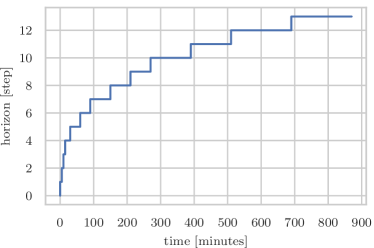
Figure 4: The $\Delta t$ of each timestep increases for larger horizons. This enables to use the accuracy of the short term predictions and to capture the energy balance of the longer horizons in the optimization.

V-2 Horizon and Timesteps

In order to make optimal use of the information from the short term forecast and at the same time take the energy balance of the coming hours into account, a variable increment of $\Delta t$ over a horizon of 15h is used. For the first control points $t_{\text{control}}$ a step size of 5 minutes is chosen, which is then increased to 3 hours (see Fig. 4). This also reduces the dimension of the optimization problem, which speeds up the computation time. The optimization is run every 5 minutes ($\Delta t_{\text{opt}}$).

V-A Cost Assumptions

For the optimization process it is necessary to define the costs for each DER as well as the electricity and the battery costs. These costs are summarized in Table II. For the battery it is assumed that only the capital and the operational costs contribute to the optimization costs (taxes are neglected)[23]. For the electrical generation from the CHP the costs are assumed to be $0.10\text{\,}\text{€}\mathrm{/}{\mathrm{k}\mathrm{W}\mathrm{h}}$ [24].

The electricity price is assumed to be $0.30\text{\,}\text{€}\mathrm{/}{\mathrm{k}\mathrm{W}\mathrm{h}}$ and the feed-in tariff $0.03\text{\,}\text{€}\mathrm{/}{\mathrm{k}\mathrm{W}\mathrm{h}}$. In addition costs for the limitation of renewable generation are applied corresponding to the levelized cost of electricity [25].

TABLE II: Costs used for the optimization model.

$\kappa_{\text{batt}}$	$0.15\text{\,}\text{€}\mathrm{/}{\mathrm{k}\mathrm{W}\mathrm{h}}$
$\kappa_{\text{CHP,\,gen}}$	$0.10\text{\,}\text{€}\mathrm{/}{\mathrm{k}\mathrm{W}\mathrm{h}}$
$\kappa_{\text{CHP,\,start}}$	$0.30\text{\,}\mathrm{\text{€}}\text{/}$ p. start
$\kappa_{\text{grid,\,draw}}$	$0.30\text{\,}\text{€}\mathrm{/}{\mathrm{k}\mathrm{W}\mathrm{h}}$
$\kappa_{\text{grid,\,feedin}}$	$0.03\text{\,}\text{€}\mathrm{/}{\mathrm{k}\mathrm{W}\mathrm{h}}$
$\kappa_{\text{RES,\,curtailment}}$	$0.10\text{\,}\text{€}\mathrm{/}{\mathrm{k}\mathrm{W}\mathrm{h}}$

Figure 5: Comparison of the absolute costs of the different error scenarios with and without battery. The error bars show the $95\text{\,}\mathrm{\char 37\relax}\text{/}$ confidence intervall of the underlying data.

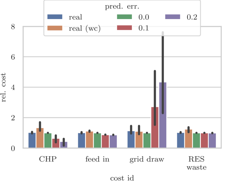
Figure 6: Comparison of the relative costs per device for the case without battery.

VI Results

To show the influence of the prediction error on scheduling applications a simulation based on the before mentioned scenarios is carried out. All results are normalized to the base case: perfect predictions ($\varepsilon_{\text{pred}}=0.0$) and no battery.

In Fig. 5 the overall costs depending on the prediction accuracy for a scenario with and without battery are shown. On the x-axis the prediction error scenarios are listed and on the y-axis the costs relative to a scenario without prediction error nor battery are displayed. The first error scenario shows the costs based on real predictions generated with neural networks. The second item describes a worst case scenario based on real predictions (robust optimization). This is the most conservative scenario which is supposed to ensure a save operation of the plant in presence of prediction errors. The following columns describe synthetic prediction scenarios with a RMSE of $0.0$, $0.1$ and $0.2$ relative to the maximum value of the profile. The error was modeled using the fit described in equation (7) normalized to the maximum power of the corresponding unit.

VI-A Sensitivity on the prediction error

Figure 7: Comparison of the relative costs per device for the case with a battery. All costs are rekative to the reference case except the battery costs: they are normalized to the scenario with perfect prediction and a battery. A enlarged version is provided in Fig 8.

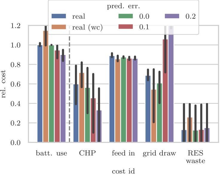
Figure 8: Enlarged version of Fig 7. Comparison of the relative costs per device for the case with battery.

In Fig. 5 it can be observed that the costs increase with a decreasing prediction accuracy. One reason for this is due to the delayed start-up behavior of the CHP unit: The controller must request the required power 15 minutes before the call time so that there is enough time for the co-generation unit to start up. This can also be seen in Fig. 6, where the costs per device for a scenario without a battery are shown. The use of the CHP declines with increasing prediction error. At the same time the amount of energy drawn from the grid increases to compensate the shortage of energy from the CHP. The amount of curtailed renewable generation (RES waste) is about the same for all scenarios.

The same plot is shown in Fig 7 for a scenario with a 20kWh battery. Compared to the scenario without a battery very little RES energy has to be curtailed as the excess can be stored in the battery.

The battery usage itself decreases with an increasing prediction error. As an increased battery usage also raises the operation costs it is only used when it is predicted to be beneficial for the total costs over the optimization horizon. If these predictions overestimate the local generation and underestimate the local demand, the battery usage decreases.

In all cases the use of a battery decreases the overall costs as the battery round trip price per kWh is in this scenario cheaper than buying electricity from the grid. Furthermore, the battery can compensate the effect of prediction errors to some extend: the costs for $\varepsilon_{\text{pred}}=0.1$ are almost the same as for the case with $\varepsilon_{\text{pred}}=0.0$ and the required power supply from the mains can be reduced.

The real predictions perform around $5\text{\,}\mathrm{\char 37\relax}\text{/}$ worse compared to the perfect predictions ($\varepsilon_{\text{pred}}=0.0$). The worst case scenario creates the highest costs but provides also the highest operational safety.

VI-B Robust optimization

For the robust optimization the worst case estimate for the prediction error is used for the optimization. This ensures a failsave operation despite the presence of prediction errors. In Fig. 7 the costs per device relative to the case with perfect predictions are shown. The worst case prediction shows the largest CHP usage and the least grid draw. This is due to the worst case optimization: as the CHP exhibits a deadtime of 15 minutes it will be switched on if the predicted profiles show any sign of a negative energy balance which could exceed the grid limits. This leads also to the larger use of the battery (see Fig. 8), as the all excess of energy is stored in the battery before fed into the grid. Furthermore, the amount of energy supplied by the grid is less than for any other strategy, which shows the robustness of the approach. One further drawback is the increased amount of curtailed renewable energy.

VII Conclusion

The results presented in this paper show the importance of accurate forecasts for smart-grid or micro-grid operations. For the presented scenario without a battery a relative prediction error of $10\text{\,}\mathrm{\char 37\relax}\text{/}$ leads to an $8\text{\,}\mathrm{\char 37\relax}\text{/}$ increase in operational costs and a $20\text{\,}\mathrm{\char 37\relax}\text{/}$ prediction error leads to an increase of about $25\text{\,}\mathrm{\char 37\relax}\text{/}$. If a battery is added to the system a relative prediction error of $10\text{\,}\mathrm{\char 37\relax}\text{/}$ leads approximately to an $2\text{\,}\mathrm{\char 37\relax}\text{/}$ increase in operational costs and a $20\text{\,}\mathrm{\char 37\relax}\text{/}$ error leads to an increase of about $30\text{\,}\mathrm{\char 37\relax}\text{/}$ respectively.

Especially if devices with a start-up time delay are included in the system, an accurate short term power prediction is needed. The effects of the prediction error can be reduced if a battery is used. If a large error margin is required (e.g. for critical facilities running in an environment with tight grid constraints) a robust optimization can be performed. This increases the failure safety of the operation but also increases the costs.

Also for storage operation a high quality forecast is important to use the battery efficiently.

References

- [1] Kerstine Appunn, Felix Bieler and Julian Wettengel “Germany’s energy consumption and power mix in charts”, 2018 URL: https://www.cleanenergywire.org/factsheets/germanys-energy-consumption-and-power-mix-charts#dossier-references
- [2] E. Moreci, G. Ciulla and V. Lo Brano “The Energy System of Sicilian Region, Italy: 2014 situation and evolutionary trends” In 2015 International Conference on Renewable Energy Research and Applications (ICRERA) Palermo, Italy: IEEE, 2015, pp. 1348–1353 DOI: 10.1109/ICRERA.2015.7418628
- [3] Hao Wang and Jianwei Huang “Hybrid renewable energy investment in microgrid” IEEE, 2014, pp. 602–607 DOI: 10.1109/SmartGridComm.2014.7007713
- [4] Mir Hadi Athari and Zhifang Wang “Modeling the uncertainties in renewable generation and smart grid loads for the study of the grid vulnerability” IEEE, 2016, pp. 1–5 DOI: 10.1109/ISGT.2016.7781265
- [5] Kazuki Ogimi et al. “Optimal operation method of wind farm with demand response” In 2012 International Conference on Renewable Energy Research and Applications (ICRERA) Nagasaki, Japan: IEEE, 2012, pp. 1–6 DOI: 10.1109/ICRERA.2012.6477328
- [6] Andrea Scalfati, Diego Iannuzzi, Maurizio Fantauzzi and Mariacristina Roscia “Optimal sizing of distributed energy resources in smart microgrids: A mixed integer linear programming formulation” In 2017 IEEE 6th International Conference on Renewable Energy Research and Applications (ICRERA) San Diego, CA: IEEE, 2017, pp. 568–573 DOI: 10.1109/ICRERA.2017.8191125
- [7] Michele Anatone and Valentina Panone “A comprehensive model for the optimal design and management of Distributed Generation systems” In 2015 International Conference on Renewable Energy Research and Applications (ICRERA) Palermo, Italy: IEEE, 2015, pp. 1451–1456 DOI: 10.1109/ICRERA.2015.7418648
- [8] Xiaohong Guan, A. Svoboda and Chao-An Li “Scheduling hydro power systems with restricted operating zones and discharge ramping constraints” In IEEE Transactions on Power Systems 14.1, 1999, pp. 126–131 DOI: 10.1109/59.744500
- [9] Earl E. Bomberger “A Dynamic Programming Approach to a Lot Size Scheduling Problem” In Management Science 12.11, 1966, pp. 778–784 DOI: 10.1287/mnsc.12.11.778
- [10] S.J. Wang et al. “Short-term generation scheduling with transmission and environmental constraints using an augmented Lagrangian relaxation” In IEEE Transactions on Power Systems 10.3, 1995, pp. 1294–1301 DOI: 10.1109/59.466524
- [11] Xiang Yu and Hui Sun “Unit commitment by enhanced adaptive Lagrangian relaxation with an improved unit substitution heuristic” IEEE, 2016, pp. 5–9 DOI: 10.1109/IMCEC.2016.7867102
- [12] T.O. Ting, M.V.C. Rao and C.K. Loo “A Novel Approach for Unit Commitment Problem via an Effective Hybrid Particle Swarm Optimization” In IEEE Transactions on Power Systems 21.1, 2006, pp. 411–418 DOI: 10.1109/TPWRS.2005.860907
- [13] K.. Dahal, J.. McDonald and G.. Burt “Modern heuristic techniques for scheduling generator maintenance in power systems” In Transactions of the Institute of Measurement and Control 22.2, 2000, pp. 179–194 DOI: 10.1177/014233120002200204
- [14] Steven Diamond and Stephen Boyd “CVXPY: A Python-Embedded Modeling Language for Convex Optimization” In Journal of Machine Learning Research 17.83, 2016, pp. 1–5
- [15] Steven Diamond Akshay Agrawal and Stephen Boyd “A Rewriting System for Convex Optimization Problems” In Journal of Control and Decision 5.1, 2018, pp. 42–60
- [16] Kai Heussen, Stephan Koch, Andreas Ulbig and Goran Andersson “Energy storage in power system operation: The power nodes modeling framework” IEEE, 2010, pp. 1–8 DOI: 10.1109/ISGTEUROPE.2010.5638865
- [17] Morales-Espana, Jesus M. Latorre and Andres Ramos “Tight and Compact MILP Formulation for the Thermal Unit Commitment Problem” In IEEE Transactions on Power Systems 28.4, 2013, pp. 4897–4908 DOI: 10.1109/TPWRS.2013.2251373
- [18] German Morales-Espana, Andres Ramos and Javier Garcia-Gonzalez “An MIP Formulation for Joint Market-Clearing of Energy and Reserves Based on Ramp Scheduling” In IEEE Transactions on Power Systems 29.1, 2014, pp. 476–488 DOI: 10.1109/TPWRS.2013.2259601
- [19] Deepak Rajan and Samer Takriti “Minimum Up/Down polytopes of the Unit Commitment Problem with Start-Up Cost”, 2005 URL: https://domino.research.ibm.com/library/cyberdig.nsf/papers/CDCB02A7C809D89E8525702300502AC0/$File/rc23628.pdf
- [20] Matt Wytock, Nicholas Moehle and Stephen Boyd “Dynamic energy management with scenario-based robust MPC” IEEE, 2017, pp. 2042–2047 DOI: 10.23919/ACC.2017.7963253
- [21] Martin Felder, Anton Kaifel and Alex Graves “Wind power prediction using mixture density recurrent neural networks”, 2010
- [22] Wahiba Yaici et al. “Artificial neural network modelling for performance prediction of solar energy system” In 2015 International Conference on Renewable Energy Research and Applications (ICRERA) Palermo, Italy: IEEE, 2015, pp. 1147–1151 DOI: 10.1109/ICRERA.2015.7418589
- [23] “LAZARD ’s Levelized Cost of Storage Analysis – Version 3.0”, 2017 URL: https://www.lazard.com/media/450338/lazard-levelized-cost-of-storage-version-30.pdf
- [24] Tien Nguyen, Jacob Spendelow and Robert Margolis “Levelized Costs of Electricity from CHP and PV”, 2014 URL: https://www.hydrogen.energy.gov/pdfs/14003_lcoe_from_chp_and_pv.pdf
- [25] Christoph Kost and Thomas Schlegl “Levelized Cost of Electricity- Renewable Energy Technologies”, 2018 URL: https://www.ise.fraunhofer.de/en/publications/studies/cost-of-electricity.html