Multi-level integration for meson propagators

Abstract:

The computation of many correlation functions in lattice QCD is severely hindered by a signal-to-noise problem. Recent developments in the factorization of both the fermion propagator and determinant pave the way for the implementation of multi-level Monte Carlo integration techniques for lattice QCD. In these proceedings we introduce new strategies for the estimation of the factorized contribution to the connected and disconnected diagrams for meson two-point functions. An estimator for the factorized connected diagram is constructed sequentially for a two-level integration scheme. For the disconnected diagram, we introduce an improved estimator by performing a frequency-splitting of traces, applicable with or without multi-level integration. Preliminary results in the quenched theory with a two-level integration scheme are presented.
DESY 18-186

1 Introduction

In the context of lattice Quantum Chromodynamics (QCD), numerical computations of correlation functions suffer from the fact that the signal decreases with the distance exponentially faster that the statistical error [1, 2]. This well-known signal-to-noise ratio problem currently limits the precision of several determinations, such as the hadronic vacuum polarization contribution (HVP) to the muon $g-2$, masses and matrix elements of baryon states, amplitudes of leptonic and semi-leptonic $B$ meson decays and many others.

A possible solution to this problem can be found in the framework of multi-level integration techniques: if the action and the observable can be factorized, independent measurements on different domains can be combined together, so that the noise decreases with the distance exponentially faster with respect to a standard Monte Carlo simulation. In the context of pure-gauge theories, this approach has proved to work extremely well [3, 4, 5, 6, 7, 8], essentially either taming or completely solving the problem.

However, the non-locality of both the determinant and the quark propagator makes an extension to fermionic theories highly non-trivial. In the last few years a conceptual advancement in this direction [9, 10, 11, 12] provided the theoretical framework for an implementation of multi-level techniques in full QCD. In this contribution we focus on recent developments in this line of research for the computation of the observables in a multi-level fashion by introducing novel techniques to calculate both connected and disconnected two-point functions.

For what concerns the connected diagrams, we exploit the possibility of placing random sources on a time-slice in between the source and the sink so to compute the two-point function using a sequential propagator. In this approach the average over the first region can be easily taken, thus paving the way for a two-level simulation with two domains.

In the case of disconnected diagrams, we introduce a new variance-reduction strategy for the computation of disconnected quark loops, which can also be applied to ordinary QCD simulations. Then we investigate the disconnected diagram for the meson two-point function in a two-level simulation, and confirm that a simple factorization scheme [9] is applicable also in the case of the two-point function of the vector current.

These proceedings are structured as follows: in section 2 we analyse the signal-to-noise ratio problem and its possible solution in the form of multi-level simulations, while in section 3 we introduce the factorization of the quark propagator first proposed in [9]. Sections 4 and 5 represent the main contribution of these proceedings, in which we present the latest developments concerning the computation of connected and disconnected diagrams in a multi-level simulation. Finally, in section 6 we draw some conclusions.

2 Signal-to-noise ratios and multi-level integration

A typical example is a meson correlation function at non-zero momentum $\bf p$, which at large enough source-sink separation $\lvert y_{0}-x_{0}\rvert$ is

$$C_{\Gamma}(x_{0},y_{0},{\bf p})\propto\exp\left[-E_{\Gamma}({\bf p})\lvert y_{0}-x_{0}\rvert\right]$$ (1)

while the variance of this object decays with the lightest state with four quark lines, e.g. the two-pion state

$$\sigma^{2}_{\Gamma}(x_{0},y_{0},{\bf p})\propto\exp\left[-2M_{\pi}\lvert y_{0}-x_{0}\rvert\right]$$ (2)

leading to an exponentially vanishing signal-to-noise ratio,

$$\frac{C_{\Gamma}(x_{0},y_{0},{\bf p})}{\sigma_{\Gamma}(x_{0},y_{0},{\bf p})/\sqrt{n}}\propto\sqrt{n}\,\exp\left[-(E_{\Gamma}({\bf p})-M_{\pi})\lvert y_{0}-x_{0}\rvert\right],$$ (3)

where $n$ is the number of gauge configurations.

In a multi-level Monte Carlo simulation the observable is sampled in two (or more) levels: at level-0, $n_{0}$ configurations are generated as in a standard computation; at level-1, for each level-0 configuration $n_{1}$ configurations are generated by updating independently different space-time regions using the factorized action. Eventually, the factorized estimator of the observable, such as a two-point function, for a two-level simulation over $m$ domains can be written as

$$C^{\text{(f)}}_{\Gamma}(x_{0},y_{0},{\bf p})\simeq\frac{1}{n_{0}}\sum_{i=1}^{n_{0}}\left[O_{1}\right]_{n_{1}}\left[O_{2}\right]_{n_{1}}...\left[O_{m}\right]_{n_{1}}$$ (4)

where each term of the type $\left[O_{k}\right]_{n_{1}}$ represents the inner level-1 average over the $k$-th space-time region. Ideally, the standard error of this estimator would then scale like $n_{0}^{-1/2}n_{1}^{-m/2}$, thus enhancing exponentially the signal-to-noise ratio of eq. 3.

3 Factorization of quark propagator

We are interested in the factorization of the quark propagator $Q^{-1}(y,x)$, a non-local functional of the gauge field over the entire lattice. Following [9, 11], we start by introducing in the temporal direction three non-overlapping domains $\Lambda_{i}$ ($i=1,2,3$) that encompass the full lattice; in this particular decomposition the domain $\Lambda_{0}\cup\Lambda_{2}$ is a disconnected one (i.e. $\Lambda_{0}$ and $\Lambda_{2}$ do not touch). In the following we will refer to $\Lambda_{1}$ as the “frozen” region, while to $\Lambda_{0}$ and $\Lambda_{2}$ as the “active” regions.

In this geometrical setup the Hermitian Wilson-Dirac operator can be written in block form as

$$Q=\begin{pmatrix}Q_{\Lambda_{0,0}}&Q_{\Lambda_{0,1}}&0\\ Q_{\Lambda_{1,0}}&Q_{\Lambda_{1,1}}&Q_{\Lambda_{1,2}}\\ 0&Q_{\Lambda_{2,1}}&Q_{\Lambda_{2,2}}\\ \end{pmatrix}.$$ (5)

A possible, simple decomposition is defined by taking the overlapping domains $\Omega_{i}^{*}=\Lambda_{i}\cup\Lambda_{i+1}$, so that in each of them the $Q$ operator becomes

$$Q_{\Omega_{i}^{*}}=\begin{pmatrix}Q_{\Lambda_{i,i}}&Q_{\Lambda_{i,i+1}}\\ Q_{\Lambda_{i+1,i}}&Q_{\Lambda_{i+1,i+1}}\\ \end{pmatrix}.$$ (6)

It was shown in [9, 11] that the exact quark propagator from a source $x\in\Lambda_{0}$ to a sink $y\in\Lambda_{2}$ can be written as

$$Q^{-1}=-Q_{\Omega_{1}^{*}}^{-1}Q_{\Lambda_{1,0}}Q^{-1}$$ (7)

or, equivalently

$$Q^{-1}=-Q_{\Omega_{1}^{*}}^{-1}Q_{\Lambda_{1,0}}\frac{1}{1-\omega}Q_{\Omega_{0}^{*}}^{-1}$$ (8)

where the operator $\omega$ is defined as $\omega=Q_{\Omega_{0}^{*}}^{-1}Q_{\Lambda_{1,2}}Q_{\Omega_{1}^{*}}^{-1}Q_{\Lambda_{1,0}}$. It is crucial to observe that the dependence on the gauge fields of the two overlapping domains is made explicit. By taking the first term of the geometric series of eq. 8, one can write an approximate, fully-factorized version of the propagator as

$$Q^{-1}\simeq-Q_{\Omega_{1}^{*}}^{-1}Q_{\Lambda_{1,0}}Q_{\Omega_{0}^{*}}^{-1}.$$ (9)

On the other hand, in the case of $x,y\in\Lambda_{0}$ one can write the quark propagator as

$$Q^{-1}=Q_{\Omega_{0}^{*}}^{-1}+Q_{\Omega_{0}^{*}}^{-1}Q_{\Lambda_{1,2}}Q_{\Omega_{1}^{*}}^{-1}Q_{\Lambda_{1,0}}\frac{1}{1-\omega}Q_{\Omega_{0}^{*}}^{-1}$$ (10)

which is instrumental for the computation of disconnected diagrams.

4 Connected diagrams

We study the correlation function $C_{\Gamma}$ of two non-diagonal quark densities

$$C_{\Gamma}(y_{0},x_{0})=\frac{a^{6}}{L^{3}}\sum_{\mathbf{x},\mathbf{y}}\langle\overline{d}(y)\Gamma u(y)\,\overline{u}(x)\Gamma d(x)\rangle=-\frac{a^{6}}{L^{3}}\sum_{\mathbf{x},\mathbf{y}}\langle W_{\Gamma}(y,x)\rangle$$ (11)

where $W_{\Gamma}(y,x)$ is the Wick contraction

$$W_{\Gamma}(y,x)=\operatorname{Tr}\left\{Q^{-1}(y,x)\Gamma\left[Q^{-1}(y,x)\right]^{\dagger}\Gamma\right\}.$$ (12)

In this section we present the definition of a new estimator of the meson correlator with stochastic sources: indeed, if we rewrite the quark propagator $Q^{-1}$ as in eq. (7) we obtain

$$W_{\Gamma}(y,x)=\operatorname{Tr}\left\{Q_{\Lambda_{1,0}}\,Q^{-1}(\cdot,x)\,\Gamma\,Q^{-1}(x,\cdot)\,Q_{\Lambda_{0,1}}\,Q_{\Omega_{1}^{*}}^{-1}(\cdot,y)\,\Gamma\,Q_{\Omega_{1}^{*}}^{-1}(y,\cdot)\right\}.$$ (13)

Upon closer inspection of eq. (13), it is clear that the standard choice of positioning the random vectors at the coordinate $x_{0}$, i.e. the time-slice on which the source is located (as in eq. (11)), is not the only one. In fact, one could place them on the interior boundary of the $\Lambda_{0}$ domain, i.e. exactly on the time slice next to the second domain $\Lambda_{1}$, and thus introduce a new estimator for the two-point function.

Furthermore, if we use the approximate quark propagator of eq. (9) we can introduce a fully factorized meson correlation function whose contraction is

$$W^{\text{(f)}}_{\Gamma}(y,x)=\operatorname{Tr}\left\{\left[Q_{\Lambda_{1,0}}\,Q_{\Omega_{0}^{*}}^{-1}(\cdot,x)\,\Gamma\,Q_{\Omega_{0}^{*}}^{-1}(x,\cdot)\,Q_{\Lambda_{0,1}}\right]\left[\,Q_{\Omega_{1}^{*}}^{-1}(\cdot,y)\,\Gamma\,Q_{\Omega_{1}^{*}}^{-1}(y,\cdot)\right]\right\}$$ (14)

where one can easily note that the term $Q_{\Omega_{0}^{*}}^{-1}(\cdot,x)\,\Gamma\,Q_{\Omega_{0}^{*}}^{-1}(x,\cdot)$ involves only fields belonging to $\Omega_{0}^{*}$, while $Q_{\Omega_{1}^{*}}^{-1}(\cdot,y)\,\Gamma\,Q_{\Omega_{1}^{*}}^{-1}(y,\cdot)$ only fields belonging to $\Omega_{1}^{*}$. We stress the fact that the factorized two-point function $C^{\text{(f)}}_{\Gamma}$ obtained from eq. (14) is an approximation: an unbiased estimator for the exact correlator requires the computation of the rest, defined as

$$C^{\text{(r)}}_{\Gamma}(y_{0},x_{0})=C_{\Gamma}(y_{0},x_{0})-C^{\text{(f)}}_{\Gamma}(y_{0},x_{0}).$$ (15)

In practice, we can use the freedom in positioning the noise source to define a new estimator $\tilde{W}^{\text{(f)}}_{\Gamma}$ for the Wick contraction of the factorized two-point function, namely

$$\tilde{W}^{\text{(f)}}_{\Gamma}(y,x)=\frac{1}{N_{\eta}}\sum_{i=1}^{N_{\eta}} \sum_{\begin{subarray}{c}\bm{z},\bm{w},\bm{w^{\prime}}\\ \bm{z^{\prime\prime}},\bm{z^{\prime}}\end{subarray}}\eta_{i}(z)^{\dagger}\,Q_{\Lambda_{0,1}}(z,w)\,Q_{\Omega_{1}^{*}}^{-1}(w,y)\,\Gamma\,Q_{\Omega_{1}^{*}}^{-1}(y,w^{\prime})$$

$$\times Q_{\Lambda_{1,0}}(w^{\prime},z^{\prime\prime})\,Q_{\Omega_{0}^{*}}^{-1}(z^{\prime\prime},x)\,\Gamma\,Q_{\Omega_{0}^{*}}^{-1}(x,z^{\prime})\,\eta_{i}(z^{\prime})$$ (16)

where all the space-time coordinates have been made explicit: $z_{0}=z^{\prime}_{0}=z^{\prime\prime}_{0}$ is the time coordinate of the interior boundary of $\Lambda_{0}$, where the random vectors are located, while $w_{0}=w^{\prime}_{0}$ is the interior boundary of $\Lambda_{1}$. As usual, the random fields $\eta_{i}(x)$ ($i=1,...,N_{\eta}$) are defined such that

$$\langle\eta_{i}(x)\rangle_{\eta} =0,$$ (17)

$$\langle\eta_{i}(x)\eta_{j}(y)^{\dagger}\rangle_{\eta} =\delta_{ij}\delta_{xy}$$ (18)

where spin and colour indices have been suppressed.

The Wick contraction of eq. (4) can be computed in a Monte Carlo multi-level integration scheme by evaluating the meson propagator sequentially. The strategy of the calculation requires that the propagator matrix element (spin and colour indices are suppressed)

$$\phi_{i}(w^{\prime})=Q_{\Lambda_{1,0}}(w^{\prime},\cdot)\,Q_{\Omega_{0}^{*}}^{-1}(\cdot,x)\,\Gamma\,Q_{\Omega_{0}^{*}}^{-1}(x,\cdot)\,\eta_{i}(\cdot)$$ (19)

is computed first for each of the $n_{1}$ level-1 configurations of the $\Omega_{0}^{*}$ domain; the level-1 average $\langle\phi_{i}\rangle_{n_{1}}$ is stored for each noise vector. Then, for each of the level-1 configurations of the $\Omega_{1}^{*}$ region one computes

$$Q_{\Omega_{1}^{*}}^{-1}(y,\cdot)\,Q_{\Lambda_{1,0}}(\cdot,\cdot)\,\eta_{i}(\cdot)\qquad\text{ and }\qquad Q_{\Omega_{1}^{*}}^{-1}(y,\cdot)\,\left[\phi_{i}(\cdot)\right]_{n_{1}}$$ (20)

where $\left[\ldots\right]_{n_{1}}$ indicates the level-1 average previously computed on $\Omega_{0}^{*}$. From these two quantities the correlation function is computed at the sink $y_{0}$ averaging over the $n_{1}$ level-1 configurations.

4.1 Numerical tests for the vector correlator

In order to assess the feasibility of this technique and its effectiveness in dealing with the signal-to-noise ratio problem, a numerical study is performed in the quenched theory. In particular, we compute the factorized vector correlator at zero momentum (averaged over $\gamma_{i}$, $i=1,2,3$) both in a conventional Monte Carlo simulation, to assess the size and the error of the rest of the propagator, and in a two-level simulation, to test the effective gain in the simulation cost.

chain id	$\beta$	$L/a$	$T/a$	$\kappa$	$c_{\mathrm{sw}}$	$m_{\mathrm{PS}}$ (MeV)	$a$ (fm)
D2	$6.2$	32	96	$0.1352$	$1.61375$	$580$	$0.068$

Table 1: Numerical setup of Monte Carlo simulation test in the quenched approximation.

Using the numerical setup reported in tab. 1, $n_{0}=100$ level-0 configurations are generated with in quenched QCD with the Wilson action and periodic boundary conditions in all directions. For the generation of the level-1 configurations, the lattice is divided in the time direction into the two active regions

• $\Lambda_{0}=\{x:x_{0}\in(0,39)a\}$,

• $\Lambda_{2}=\{x:x_{0}\in(48,87)a\}$;

and into the frozen region

• $\Lambda_{1}=\{x:x_{0}\in(40,47)a\}\cup\{x:x_{0}\in(88,95)a\}$,

which is composed of two disconnected domains, each of width $\Delta=8$. For each level-0 configuration and for each active region belonging to $\Omega_{0}^{*}$ and $\Omega_{1}^{*}$, $n_{1}=16$ level-1 configurations were produced while keeping the fields in $\Lambda_{1}$ fixed. The connected two-point function is computed using $N_{\eta}=40$ noise sources placed in the interior boundaries of $\Lambda_{0}$, namely $z_{0}=0$ and $z_{0}=39a$. The factorized contribution, $C^{\text{(f)}}$, is calculated using eq. (4) both with and without multi-level integration. In order to compute the rest, $C^{\text{(r)}}$, the exact two-point function is obtained using the same noise sources for the exact propagator of eq. (7).

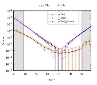
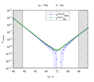
Figure 1: Left: results for the exact vector correlator (red triangles), along with the factorized contribution (blue triangles) and the rest (dark-red triangles). Right: comparison of results for the exact vector correlator calculated with a standard Monte Carlo simulation (SMC, blue triangles), and the factorized contribution computed with a multi-level integration scheme (ML, green dots).

In the left panel of fig. 1 we present results obtained with $x_{0}=24a$ for the exact two-point function, its factorized part, computed in a standard Monte Carlo (SMC), and the rest of the propagator. We first observe the appearance of the signal-to-noise ratio problem at source-sink separations $\lvert y_{0}-x_{0}\rvert$ of around 40 lattice spacings. Furthermore, the size of the rest of the propagator is relatively small, namely about 5% of the value of the exact correlation function. As long as the signal is present, the exact and factorized results agree within error. We remark that these results are obtained with all $n_{0}\times n_{1}$ configurations: since the level-1 configurations share the same frozen regions, the data analysis must be performed by binning the $n_{1}$ configurations. Then, we proceed with the extraction of results within a multi-level integration scheme: from the right panel of fig. 1 it is immediately clear how this approach is able to deal with the signal-to-noise ratio problem, drastically reducing the error while using the same $n_{0}\times n_{1}$ configurations.

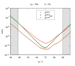
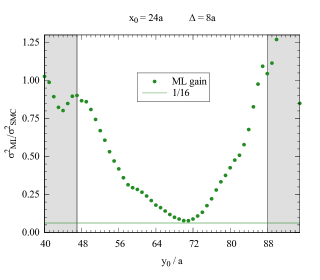
Figure 2: Left: comparison of errors associated to the factorized vector correlator with (green dots) and without (red triangles) multi-level, along with the error associated to the rest (dark-red triangles). Right: ratio between the variance obtained with a multi-level scheme and with a standard Monte Carlo simulation, on the same set of $n_{0}\times n_{1}$ configurations.

The left panel of fig. 2 clearly shows how the error is reduced by making use of the multi-level technique described in section 4. Furthermore, we can observe that, in this numerical setup, the error on the rest of the two-point function is still smaller that the error on the factorized part, even when obtained in a multi-level scheme with $n_{1}=16$. Finally, in order to understand what is the gain in terms of computational cost, one can look at the ratio of the variance obtained with a standard Monte Carlo and with a multi-level technique. The “ideal” scaling one expects would be $1/n_{1}$: in the right panel of fig. 2 we can observe that this ratio depends strongly on the distance from the frozen region, and that indeed it reaches the expected scaling of $1/n_{1}=1/16$ when far away enough from $\Lambda_{1}$.

5 Disconnected diagrams

Quark-line disconnected diagrams arise in any correlation function with fermion bilinears which contain some flavour-singlet component, such as the electromagnetic current, whose matrix elements appear in the computation of hadronic form factors, and the leading hadronic contributions to muon $g-2$. Furthermore, disconnected diagrams are also present in meson spectroscopy in isosinglet channels, and in generalized susceptibilities at finite temperature and density. Several of these observables suffer from the signal-to-noise problems described earlier and it is crucial to test multi-level methods for these correlation functions.

In the following subsection we propose a variance reduction method for the stochastic estimation of disconnected quark loops and test it numerically in a single-level quenched simulation with the same parameters used in sec. 4.1. In subsection 5.2 we investigate the disconnected contribution to the vector two-point function in a two-level simulation using the proposed variance-reduction methods.

5.1 Variance-reduction for disconnected diagrams

The disconnected quark loop is usually computed with a noisy estimator for the trace [13],

$$\operatorname{Tr}\{\Gamma S^{f}(x,x)\} \approx\begin{cases}\mathrm{Im}{T^{f}_{\Gamma}(x,x)}\quad&\textrm{if }\Gamma=\gamma_{\mu},\\ \mathrm{Re}{T^{f}_{\Gamma}(x,x)}\quad&\textrm{if }\Gamma\in\{1,\gamma_{5},\gamma_{\mu}\gamma_{5},\sigma_{\mu\nu}\},\end{cases}$$ (21)

$$T^{f}_{\Gamma}(x,x) =\frac{1}{N_{\eta}}\sum_{n=1}^{N_{\eta}}\eta_{n}^{\dagger}(x)\Gamma\sum_{y}S^{f}(x,y)\eta_{n}(y),$$ (22)

where $S=Q^{-1}\gamma_{5}$ is the $\gamma_{5}$-Hermitian quark propagator, $\Gamma$ is a Dirac matrix, and the independent components of the noise $\eta_{n}(x)$ are drawn from a $\mathrm{U}(1)$ distribution, which has zero mean and finite variance, as per eqs. (17). Although this estimator is unbiased, it converges only with $\mathrm{O}(N_{\eta}^{-1/2})$ to the expectation value, namely that its variance scales inversely proportional to the number of sources. However, in order to test the scaling of the gauge noise in a two-level integration scheme we ought to have a precise estimate of the quark loop.

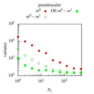
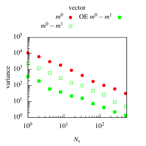
Figure 3: The variance as a function of the number of sources, $N_{\eta}$, in the pseudoscalar (left) and vector (right) channels. The red symbols represent the variance for the light quark mass while the green symbols the difference between the light and a heavier quark mass. The open and filled green symbols are two different estimators for the difference, explained in the text.

As can be seen in fig. 3, the variance of the quark loop summed on a timeslice (red circles) scales inversely to the number of sources. In the pseudoscalar channel (left), the variance begins to saturate to the gauge noise after a few hundred noise sources, while in the vector channel (right) no evidence for the reaching the gauge limit is observed. This compels us to search for an improved estimator, especially for the vector channel, for which the gauge noise has, to the best of our knowledge, never been reached.

An alternative estimator can be constructed for the single-quark loop by performing a frequency-splitting of the trace, inspired by the mass-preconditioning of the forces in the HMC [14], by constructing the telescoping sum

$$\operatorname{Tr}\{\Gamma S^{f_{0}}(x,x)\} =\operatorname{Tr}\{\Gamma(S^{f_{0}}-S^{f_{1}})(x,x)\}+\operatorname{Tr}\{\Gamma(S^{f_{1}}-S^{f_{2}})(x,x)\}+\ldots+\operatorname{Tr}\{\Gamma S^{f_{M}}(x,x)\},$$ (23)

with a hierarchy of bare quark masses $m^{f_{0}}_{0}<m^{f_{1}}_{0}<\ldots<m^{f_{M}}_{0}$. If each of the traces on the right-hand size of the equation is computed separately via

$$\operatorname{Tr}\{\Gamma(S^{f_{i}}-S^{f_{i+1}})(x,x)\} \approx\mathrm{Re}(\mathrm{Im})\left[\frac{1}{N_{\eta}}\sum_{n=1}^{N_{\eta}}\eta_{n}^{\dagger}(x)\Gamma\sum_{y}\{S^{f_{i}}(x,y)-S^{f_{i+1}}(x,y)\}\eta_{n}(y)\right],$$ (24)

then the frequency-splitting estimator effectively splits the sources of the variance from different energy scales. If the dominant contribution is from the UV part, then the noise can be controlled at larger quark masses which requires less computational effort, much like integrating the computationally intensive forces on a larger time-scale in the HMC.

Furthermore, we expect a large correlation between propagators with similar quark masses which means that the estimate eq. (24) will have a reduced variance to the single quark loop [15]. Indeed, the variance of the estimator for the difference is reduced with respect to the variance on a single trace, as can be observed in figure 3 (green open squares), where a second flavour with a large quark mass $m^{1}_{0}$ has been introduced, see tab. 2.

Another variation can be obtained by using an identity for the Wilson-Dirac operator to express the difference of a doublet of propagators with different quark masses as a product

$$S^{f_{i}}(x,y)-S^{f_{i+1}}(x,y) =(m^{f_{i+1}}_{0}-m^{f_{i}}_{0})\sum_{z}S^{f_{i+1}}(x,z)S^{f_{i}}(z,y).$$ (25)

The product on the right-hand side gives a new possibility for an estimator for difference eq. (24) via

$$\operatorname{Tr}\{\Gamma(S^{f_{i}}-S^{f_{i+1}})(x,x)\} \approx(m^{f_{i+1}}_{0}-m^{f_{i}}_{0})\times$$

$$\quad\mathrm{Re}(\mathrm{Im})\left[\frac{1}{N_{\eta}}\sum_{n=1}^{N_{\eta}}\operatorname{Tr}\{\Gamma\sum_{y,z}S^{f_{i+1}}(x,y)\eta_{n}(z)\eta^{\dagger}_{n}(z)S^{f_{i}}(z,x)\}\right].$$ (26)

While this one-end estimator (OE) has the same expectation value as eq. (24), it is clear that they are not equal sample-by-sample, and indeed they have different variances. This can be verified by a short computation of the variance in terms of the correlation functions after integrating out the noise fields. In practice, we observe a further reduction in both the pseudoscalar and vector channels using this estimator, as seen in fig. 3 (green filled squares). Using CLS $N_{\mathrm{f}}=2$ configurations, we have observed a large reduction in the variance when the quark masses are set to the light valence and strange quark masses, and therefore the application of this identity to compute the disconnected contribution to the HVP is very promising [17].

In the following we propose a frequency-splitting estimator (FS) using the one-end estimator with $M=2$ auxiliary masses, with the largest bare subtracted mass on the order of the lattice cutoff scale, see tab. 2. We employ the $k=4$ order hopping parameter expansion to evaluate the term $\operatorname{Tr}\{\Gamma S^{f_{2}}(x,x)\}$ via

$$S^{f}(x,y) =\sum_{n=0}^{k-1}H^{n}(D_{\mathrm{ee}}+D_{\mathrm{oo}})^{-1}+(H^{k}S^{f})(x,y)$$ (27)

where $H=-(D_{\mathrm{oo}}^{-1}D_{\mathrm{oe}}+D_{\mathrm{ee}}^{-1}D_{\mathrm{eo}})$ is the hopping matrix. We use either spatial dilution or hierarchical probing vectors [18] for the first ‘hopping’ terms, and a standard Monte Carlo for the remainder. The advantage of this set-up is that the stochastic noise is completely eliminated in the estimation of the hopping terms after $k^{4}/8$ quadratures, if $k/2$ is a power of two. The use of the hopping expansion in the mass-preconditioned HMC has also recently been explored in ref. [19].

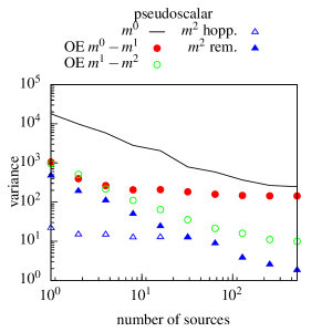
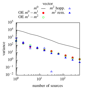
Figure 4: The variance versus the number of sources for each of the contributions to the frequency-splitting (FS) estimator (points) and the standard Monte Carlo (solid line) in the pseudoscalar (left) and vector (right) channels. Note that the hopping terms, which do not require inversions of the Dirac matrix, are computed using hierarchical probing with spin-colour dilution.

The variance of all of the components of this estimator are shown in fig. 4 as a function of the number of noise sources, along with the same for the standard stochastic estimator eq. (24) for the light quark loop (solid line). In the pseudoscalar channel, the variance on the one-end estimator for the light doublet dominates the variance (filled red circles), while in the vector channel, the hopping term is initially dominant (open blue triangles). Note that the hopping terms are estimated exactly at the right-most open triangle with $k^{4}/8=32$ quadratures.

Without any particular fine-tuning, it is a straightforward and cheap procedure to measure the variances on the each component of the FS estimator with just a few sources. In this way the cost can be optimized for a given observable. The inversions used in the estimator of the smallest quark-mass difference can be reused to create the standard estimator and compare the cost of the methods a posteriori. Furthermore, we expect that this estimator should behave well toward the chiral limit, as it effectively performs a separation of the sources of the variance at the IR and UV scales, which appears to dominate in the vector channel. In fact, as the light quark inversions become more expensive, the cost of the exact computation of the hopping terms is amortized, being independent on the quark mass.

5.2 Numerical results in the two-level integration

chain id	$m^{f}_{0}$	$\kappa$	$am_{\mathrm{q}}$
D2	$m^{0}$	0.1352	0.016
	$m^{1}$	0.128	0.224
	$m^{2}$	0.115	0.665

Table 2: The parameters used in the FS stochastic estimator for the light-quark loop. The critical hopping parameter is taken from ref. [20].

Figure 5: Graphical illustration of the unbiased estimator for the disconnected contribution to the meson two-point function in a two-level simulation. The first line is fully factorized,while the following two depend on the whole gauge field and require independent measurements for each combination of level-1 configurations for a multi-level estimator.

In this section, we apply the FS estimator proposed in the previous subsection to the disconnected two-point function in the two-level simulation described in subsection 4.1. We test an unbiased multi-level estimator for the disconnected diagram [9],

$$C_{\Gamma_{d}}(y_{0},x_{0}) =\frac{a^{6}}{L^{3}}\sum_{\bm{y},\bm{x}}\langle\operatorname{Tr}\{\gamma_{5}\Gamma Q^{-1}(y,y)\}\operatorname{Tr}\{\gamma_{5}\Gamma Q^{-1}(x,x)\}\rangle$$ (28)

where $x\in\Omega_{0}^{*}$, $y\in\Omega_{1}^{*}$, which is constructed by decomposing the hermitian propagator, $Q^{-1}$, via the identity

$$\operatorname{Tr}\{\gamma_{5}\Gamma Q^{-1}(x,x)\} =\operatorname{Tr}\{\gamma_{5}\Gamma Q^{-1}_{\Omega^{*}_{i}}(x,x)\}+\operatorname{Tr}\{\gamma_{5}\Gamma(Q^{-1}-Q^{-1}_{\Omega^{*}_{i}})(x,x)\},$$ (29)

in each of the blocks $x\in\Omega_{i}^{*}$ for $i=0,1$. This decomposition results in three contributions to the disconnected diagram,

$$C_{\Gamma_{d}}(y_{0},x_{0}) =\frac{a^{6}}{L^{3}}\sum_{\bm{y},\bm{x}}\langle(W_{\Gamma_{d}}^{(\mathrm{f})}+W_{\Gamma_{d}}^{(\mathrm{r}_{1})}+W_{\Gamma_{d}}^{(\mathrm{r}_{2})})(y,x)\rangle,$$ (30)

which are illustrated graphically in the first, second and third lines of fig. 5. The propagators $Q^{-1}_{\Omega_{i}^{*}}$ are represented by the the small blocks, while the the propagators on the whole lattice, $Q^{-1}$, are represented by the large blocks.

The contribution on the first line of the figure is therefore fully factorized, as the propagators depend only on the gauge field in the level-1 configurations respectively, and requires only $n_{0}\times~{}n_{1}$ measurements for a multi-level estimator. The other contributions depend on the gauge field in the whole lattice, and if no further factorization is introduced, a multi-level estimate would require measurements on each of the $n_{0}\times n_{1}^{2}$ combinations of level-1 configurations. Alternatively, if the variance on these non-factorized pieces is suppressed, then it may be sufficient to estimate these corrections using fewer, e.g. $n_{0}\times n_{1}$, measurements and the factorization strategy within a multi-level scheme will still be effective.

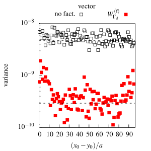
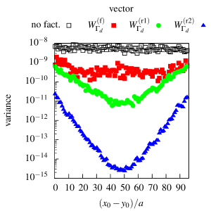
Figure 6: The variance of the vector channel disconnected diagram as a function of the source-sink separation. In the left-hand panel the variance of the non-factorized estimator using $n_{0}\times n_{1}$ configurations is compared with the factorized contribution with two-level integration (red filled squares), showing the expection $1/n_{1}=1/16$ reduction in the variance (dashed lines). In the right-hand panel, the variances of the remaining contributions (green and blue points) computed with $n_{0}\times n_{1}$ configurations is shown to be suppressed with respect to the factorized contribution.

Preliminary results for the variance with and without two-level integration are shown for the vector channel in fig. 6. In the left-hand panel, the variance of the disconnected contribution as a function of the separation $x_{0}-y_{0}$ without factorization using $n_{0}\times n_{1}$ measurements (black open squares) is compared with the variance on the factorized contribution using two-level integration (red filled squares). As expected the variance is constant in time, which gives rise to an exponentially bad signal-to-noise problem. As depicted by the dashed lines, the variance on the factorized contribution is reduced by $n_{1}=16$ using the two-level simulation. In the right-hand panel, the variance on the two remaining contributions are shown with the green and blue points. The variance is sufficiently suppressed on these remaining contributions that they remain subleading. Furthermore, the variances on these contributions appears to be exponentially suppressed with the distance.

These preliminary results indicate that a two-level scheme for the disconnected diagram in the vector channel can be easily implemented and the dominant uncertainity arises from a fully factorizable contribution.

6 Conclusions

In these proceedings we have proposed new estimators for both connected and disconnected contributions to meson two-point functions suitable for multi-level integration, and tested them in a two-level quenched simulation. Such estimators could be applied to tackle the signal-to-noise problem in, for example, singlet pseudoscalar spectroscopy, or the leading-order hadronic vacuum polarization.

For the connected diagram, a stochastic estimator for the factorized contribution is proposed which is computed sequentially in each region of the two-level simulation. As expected, the factorized contribution to the connected two-point function is a good approximation to it, and furthermore the error on the remainder is small. In the two-level simulation we have observed the expected gain over the single-level simulation when the sink is adequately far from the frozen region. The dependence of the gain on the distance from the frozen region is currently under investigation.

In the disconnected sector we have proposed a new stochastic estimator for the quark loop which is applicable with or without multi-level integration. This estimator is similar in spirit to the frequency-splitting of the quark determinant performed in the HMC, where the separation allows the dominant fluctuations to be controlled because they are less computationally intensive. In addition, we have introduced an alternative estimator for the difference of quark loops with different quark masses, which provides a signficant improvement, and could be applied to the disconnected contribution to the HVP. A detailed theoretical description of the variances using the estimators can be found in ref. [17]. Like the connected diagram, we find the variance of the factorized contribution to be dominant, which means that a factorized multi-level strategy is applicable.

The results of these new techniques confirm those presented in the previous Lattice conference [12], which were obtained with open boundary conditions, and extends them to the disconnected diagram in the vector channel. We stress that the magnitude of the correction depends heavily of the quark mass, and therefore the application of these techniques to QCD with light quarks is not straightforward.

Acknowledgements

Simulations have been performed the PC-cluster Marconi at CINECA (CINECA-INFN and CINECA-Bicocca agreements), and on the PC-cluster Wilson at Milano-Bicocca. We thankfully acknowledge the computer resources and technical support provided by these institutions.

References

- [1] G. Parisi “The Strategy for Computing the Hadronic Mass Spectrum” In COMMON TRENDS IN PARTICLE AND CONDENSED MATTER PHYSICS. PROCEEDINGS, WINTER ADVANCED STUDY INSTITUTE, LES HOUCHES, FRANCE, FEBRUARY 23 - MARCH 11, 1983 103, 1984, pp. 203–211 DOI: 10.1016/0370-1573(84)90081-4
- [2] G. Lepage “The Analysis of Algorithms for Lattice Field Theory” In Boulder ASI 1989:97-120, 1989, pp. 97–120
- [3] G. Parisi, R. Petronzio and F. Rapuano “A Measurement of the String Tension Near the Continuum Limit” In Phys. Lett. 128B, 1983, pp. 418–420 DOI: 10.1016/0370-2693(83)90930-9
- [4] Martin Lüscher and Peter Weisz “Locality and exponential error reduction in numerical lattice gauge theory” In JHEP 09, 2001, pp. 010 DOI: 10.1088/1126-6708/2001/09/010
- [5] Harvey B. Meyer “Locality and statistical error reduction on correlation functions” In JHEP 01, 2003, pp. 048 DOI: 10.1088/1126-6708/2003/01/048
- [6] Michele Della Morte and Leonardo Giusti “Exploiting symmetries for exponential error reduction in path integral Monte Carlo” In Comput. Phys. Commun. 180, 2009, pp. 813–818 DOI: 10.1016/j.cpc.2008.10.017
- [7] Michele Della Morte and Leonardo Giusti “Symmetries and exponential error reduction in Yang-Mills theories on the lattice” In Comput. Phys. Commun. 180, 2009, pp. 819–826 DOI: 10.1016/j.cpc.2009.03.009
- [8] Michele Della Morte and Leonardo Giusti “A novel approach for computing glueball masses and matrix elements in Yang-Mills theories on the lattice” In JHEP 05, 2011, pp. 056 DOI: 10.1007/JHEP05(2011)056
- [9] Marco Cè, Leonardo Giusti and Stefan Schaefer “Domain decomposition, multi-level integration and exponential noise reduction in lattice QCD” In Phys. Rev. D93.9, 2016, pp. 094507 DOI: 10.1103/PhysRevD.93.094507
- [10] Marco Cè, Leonardo Giusti and Stefan Schaefer “A local factorization of the fermion determinant in lattice QCD” In Phys. Rev. D95.3, 2017, pp. 034503 DOI: 10.1103/PhysRevD.95.034503
- [11] Leonardo Giusti, Marco Cè and Stefan Schaefer “Multi-boson block factorization of fermions” In Proceedings, 35th International Symposium on Lattice Field Theory (Lattice 2017): Granada, Spain, June 18-24, 2017 175, 2018, pp. 01003 DOI: 10.1051/epjconf/201817501003
- [12] Marco Cè, Leonardo Giusti and Stefan Schaefer “Local multiboson factorization of the quark determinant” In Proceedings, 35th International Symposium on Lattice Field Theory (Lattice 2017): Granada, Spain, June 18-24, 2017 175, 2018, pp. 11005 DOI: 10.1051/epjconf/201817511005
- [13] M.F. Hutchinson “A stochastic estimator of the trace of the influence matrix for laplacian smoothing splines” In Communications in Statistics - Simulation and Computation 19.2 Taylor & Francis, 1990, pp. 433–450 DOI: 10.1080/03610919008812866
- [14] M. Hasenbusch and K. Jansen “Speeding up lattice QCD simulations with clover improved Wilson fermions” In Nucl. Phys. B659, 2003, pp. 299–320 DOI: 10.1016/S0550-3213(03)00227-X
- [15] Harvey B. Meyer and Hartmut Wittig “Lattice QCD and the anomalous magnetic moment of the muon”, 2018 arXiv:1807.09370 [hep-lat]
- [16] Philippe Boucaud “Dynamical Twisted Mass Fermions with Light Quarks: Simulation and Analysis Details” In Comput. Phys. Commun. 179, 2008, pp. 695–715 DOI: 10.1016/j.cpc.2008.06.013
- [17] Leonardo Giusti, Tim Harris, Alessandro Nada and Stefan Schäfer “Improved estimators for disconnected loops” In In preparation, 2018
- [18] Andreas Stathopoulos, Jesse Laeuchli and Kostas Orginos “Hierarchical probing for estimating the trace of the matrix inverse on toroidal lattices”, 2013 arXiv:1302.4018 [hep-lat]
- [19] Martin Hasenbusch “Exploiting the hopping parameter expansion in the hybrid Monte Carlo simulation of lattice QCD with two degenerate flavors of Wilson fermions” In Phys. Rev. D97.11, 2018, pp. 114512 DOI: 10.1103/PhysRevD.97.114512
- [20] Martin Lüscher et al. “Nonperturbative O(a) improvement of lattice QCD” In Nucl. Phys. B491, 1997, pp. 323–343 DOI: 10.1016/S0550-3213(97)00080-1