Computational efficiency of numerical integration methods for the tangent dynamics of many-body Hamiltonian systems in one and two spatial dimensions

Abstract

We investigate the computational performance of various numerical methods for the integration of the equations of motion and the variational equations for some typical classical many-body models of condensed matter physics: the Fermi-Pasta-Ulam-Tsingou (FPUT) chain and the one- and two-dimensional disordered, discrete nonlinear Schrödinger equations (DDNLS). In our analysis we consider methods based on Taylor series expansion, Runge-Kutta discretization and symplectic transformations. The latter have the ability to exactly preserve the symplectic structure of Hamiltonian systems, which results in keeping bounded the error of the system’s computed total energy. We perform extensive numerical simulations for several initial conditions of the studied models and compare the numerical efficiency of the used integrators by testing their ability to accurately reproduce characteristics of the systems’ dynamics and quantify their chaoticity through the computation of the maximum Lyapunov exponent. We also report the expressions of the implemented symplectic schemes and provide the explicit forms of the used differential operators. Among the tested numerical schemes the symplectic integrators $ABA864$ and $SRKN^{a}_{14}$ exhibit the best performance, respectively for moderate and high accuracy levels in the case of the FPUT chain, while for the DDNLS models $s9\mathcal{ABC}6$ and $s11\mathcal{ABC}6$ (moderate accuracy), along with $s17\mathcal{ABC}8$ and $s19\mathcal{ABC}8$ (high accuracy) proved to be the most efficient schemes.

1 Introduction

A huge number of important problems in physics, astronomy, chemistry, etc. are modeled via sets of ordinary differential equations (ODEs) governed by the Hamiltonian formalism. Due to non-integrability, the investigation of the time evolution of these problems, and generally their properties, often rely solely on numerical techniques. As modern research requires numerical simulations to be pushed to their very limit (e.g. large integration times, macroscopic limits), a methodical assessment of the properties of different numerical methods becomes a fundamental issue. Such studies allow to highlight the most suitable scheme for both general purposes and specific tasks, according to criteria of stability, accuracy, simplicity and efficiency.

The beginning of the era of computational physics is considered to be the computer experiment performed in the 1950s by Fermi, Pasta, Ulam and Tsingou (FPUT) [1, 2, 3] to observe energy equipartition due to weak-anharmonic coupling in a set of harmonic oscillators. Indeed, the breaking of integrability in Hamiltonian systems is often performed with the introduction of nonlinear terms in the equations of motion. These additional nonlinear terms describe new physical processes, and led to important questions and significant advancements in condensed matter physics. For instance, the FPUT problem has been used to answer questions related to ergodicity, dynamical thermalization and chaos occurrence (see e.g. [4, 5, 6] and references therein) and led to the observation of solitons [7, 8], and progress in Hamiltonian chaos [9]. The interested reader can find a concise review of numerical results concerning the FPUT system in [10].

Another important example concerns disordered media. In 1958, Anderson [11] theoretically showed the appearance of energy localization in one-dimensional lattices with uncorrelated disorder (a phenomenon which is now referred to as Anderson localization). This phenomenon was later investigated also for two-dimensional lattices [12]. An important question which has attracted wide attention in theory, numerical simulations and experiments is what happens when nonlinearity (which appears naturally in real world problems) is introduced in a disordered system [13, 14, 15, 16, 17, 18, 19, 20, 21, 22, 23, 24, 25, 26, 27, 28, 29, 30].

Two basic Hamiltonian models are at the center of these investigations: the disordered Klein-Gordon (DKG) chain and the disordered, discrete nonlinear Schrödinger equation (DDNLS). In Refs. [22, 23, 24, 25, 26, 28, 29, 30, 31, 32, 33, 34] it was shown that Anderson localization is destroyed by the presence of nonlinearity, resulting to the subdiffusive spreading of energy due to deterministic chaos. Such results rely on the accurate, long time integration of the systems’ equations of motion and variational equations. We note that the variational equations are a set of ODEs describing the time evolution of small deviations from a given trajectory, something which is needed for the computation of chaos indicators like the maximum Lyapunov exponent (mLE) [35, 36, 37]. The numerical integration of these sets of ODEs can be performed by any general purpose integrator. For example Runge-Kutta family schemes are still used [38, 39]. Another category of integrators is the so-called symplectic integrators (SIs), which were particularly designed for Hamiltonian systems (see e.g. [40, 41, 42, 43, 44] and references therein). The main characteristic of SIs is that they conserve the symplectic structure of Hamiltonian systems, so that the numerical approximation they provide corresponds to the exact solution of a system which can be considered as a perturbation of the original one. Consequently the error in the computed value of the Hamiltonian function (usually refereed to as the system’s energy) is kept almost constant over long integration times. This almost constant error can be used as an indicator of the accuracy of the used integration scheme.

SIs have been successfully implemented for the long time integration of multidimensional Hamiltonian systems like the $\alpha$- and $\beta$-FPUT systems and FPUT-like models, the DKG, the DDNLS and systems of coupled rotors (see e.g. [22, 23, 24, 25, 26, 28, 29, 30, 32, 33, 45, 46, 47, 48, 49, 50, 51, 52, 53, 54]). In these studies SIs belonging to the so-called SABA family [55] were mostly used, since the FPUT, the DKG and systems of coupled rotors can be split into two integrable parts (the system’s kinetic and the potential energy), while in some more recent studies [33, 56] the $ABA864$ [57] SI was implemented as it displayed an even better performance. As the DDNLS model is not explicitly decomposed into two integrable parts, the implementation of SABA schemes requires a special treatment involving the application of fast Fourier transforms which are computationally time consuming [29]. In [49, 50] it was shown that for the DDNLS model, the split of the Hamiltonian function into three integrable parts is possible, and this approach proved to be the best choice for the model’s integration with respect to both speed and accuracy. It is worth noting here that the numerical integration of the variational equations by SIs is done by the so-called Tangent Map Method [58, 59, 60].

The intention of this work is to present several efficient (symplectic and non-symplectic) integration techniques for the time evolution of both the equations of motion and the variational equations of multidimensional Hamiltonian systems. In particular, in our study we use these techniques to investigate the chaotic dynamics of the one-dimensional (1D) FPUT system, as well as one- and two-dimensional (2D) DDNLS models. We carry out this task by considering particular initial conditions for both the systems and for the deviation vectors, which we evolve in time requiring a predefined level of energy accuracy. Then, we record the needed CPU time to perform these numerical simulations and highlight those methods that ensure the smallest CPU times for obtaining accurate results. A similar analysis for the 1D and 2D DKG systems was performed in [56].

The paper is organized as follows. In Sec. 2 we introduce the models considered in our study. In Sec. 3 we introduce in detail the symplectic and non-symplectic schemes implemented in our investigations. In Sec. 4 we present our numerical results and report on the efficiency of each studied scheme. In Sec. 5 we review our findings and discuss the outcomes of our study. Finally, in Appendix A we provide the explicit forms of the used tangent map operators. Moreover, we present there the explicit expressions of the tangent map operators for some additional important many-body systems, the so-called $\beta$-FPUT chain, the KG system and the classical XY model (a Josephson junction chain - JJC) in order to facilitate the potential application of SIs for these systems from the interested reader, although we do not present numerical results for these models.

2 Models and Hamiltonian functions

In this work we focus our analysis on the 1D FPUT system and the 1D and 2D DDNLS models. In what follows we briefly present the Hamiltonian functions of these systems.

2.1 The $\alpha$-Fermi-Pasta-Ulam-Tsingou model

The 1D FPUT model [1, 2, 3] was first introduced in 1955 to study the road toward equilibrium of a chain of harmonic oscillators in the presence of weak anharmonic interactions. Since then, this system has been widely used as a toy model for investigating energy equipartition and chaos in nonlinear lattices. In the literature there exist two types of the FPUT model the so-called $\alpha-$ and $\beta-$FPUT systems. In our study we consider the $\alpha-$FPUT model whose Hamiltonian function reads

$$H_{\text{1F}}=\sum_{i=0}^{N}\left[\frac{p_{i}^{2}}{2}+\frac{1}{2}(q_{i+1}-q_{i})^{2}+\frac{\alpha}{3}(q_{i+1}-q_{i})^{3}\right].$$ (2.1)

In Eq.(2.1), $q_{i}$ and $p_{i}$ are respectively the generalized coordinates and momenta of the $i$ lattice site and $\alpha$ is a real positive parameter. In our study we consider fixed boundary conditions $q_{0}=p_{0}=p_{N+1}=q_{N+1}=0$. We also note that this model conserves the value of the total energy $H_{\text{1F}}$.

In contrast to the $\alpha$-FPUT system, the $\beta$-FPUT model is characterized by a quartic nonlinear term [see Eq. (A.26) in Appendix A.4]. The fact that the value of the Hamiltonian function of the $\beta$-FPUT model is bounded from below leads to differences between the two models. For example, phenomena of chopping time which occur in the $\alpha$- model do not appear in the $\beta$-FPUT system [61]. Further discussion of the differences between the $\alpha$- and the $\beta$- models can be found in [62, 63, 64].

2.2 The 1D and 2D disordered discrete nonlinear Schrödinger equations

The DDNLS model describes anharmonic interactions between oscillators in disordered media and has been used to study the propagation of light in optical media or Bose-Einstein condensates through the famous Gross-Pitaevskii equation [52], as well as investigate, at a first approximation, several physical processes (e.g. electron tight binding systems [39]). The Hamiltonian function of the 1D DDNLS model reads

$$H_{1D}=\sum_{i=1}^{N}\left[\frac{\epsilon_{i}}{2}(q_{i}^{2}+p_{i}^{2})+\frac{\beta}{8}(q_{i}^{2}+p_{i}^{2})^{2}-p_{i+1}p_{i}-q_{i+1}q_{i}\right],$$ (2.2)

where $q_{i}$ and $p_{i}$ are respectively the generalized coordinates and momenta of the $i$ lattice site and the onsite energy terms $\epsilon_{i}$ are uncorrelated numbers uniformly distributed in the interval $\left[-\frac{W}{2},\frac{W}{2}\right]$. The real, positive numbers $W$ and $\beta$ denote the disorder and the nonlinearity strength respectively. We also consider here fixed boundary conditions i.e. $q_{0}=p_{0}=p_{N+1}=q_{N+1}=0$.

The two-dimensional version of the DDNLS model was considered in [30, 65]. Its Hamiltonian function is

$$H_{2D}=\sum_{i=1}^{N}\sum_{j=1}^{M}\bigg{\{}\frac{\epsilon_{i,j}}{2}\left[q_{i,j}^{2}+p_{i,j}^{2}\right]+\frac{\beta}{8}\left[q_{i,j}^{2}+p_{i,j}^{2}\right]^{2}-\left[q_{i,j+1}q_{i,j}+q_{i+1,j}q_{i,j}+p_{i,j+1}p_{i,j}+p_{i+1,j}p_{i,j}\right]\bigg{\}},$$ (2.3)

where $q_{i,j}$ and $p_{i,j}$ are respectively the generalized positions and momenta at site $(i,j)$ and $\epsilon_{i,j}$ are the disorder parameters uniformly chosen in the interval $\left[-\frac{W}{2},\frac{W}{2}\right]$. We again consider fixed boundary conditions i.e. $q_{0,j}=p_{0,j}=q_{N+1,j}=p_{N+1,j}=0$ for $1\leq j\leq M$ and $q_{i,0}=p_{i,0}=q_{i,M+1}=p_{i,M+1}=0$ for $1\leq i\leq N$.

Additionally to the energies $H_{1D}$ [Eq. (2.2)] and $H_{2D}$ [Eq. (2.3)] both systems conserve their respective norms $S_{\text{1D}}$ and $S_{\text{2D}}$:

$$S_{\text{1D}}=\frac{1}{2}\sum_{i=1}^{N}\left(q_{i}^{2}+p_{i}^{2}\right)\ ;\qquad\quad S_{\text{2D}}=\frac{1}{2}\sum_{i=1}^{N}\sum_{j=1}^{M}\left(q_{i,j}^{2}+p_{i,j}^{2}\right)\ .$$ (2.4)

3 Numerical integration schemes

The Hamilton equations of motion

$$\frac{d\boldsymbol{q}}{dt}=\frac{\partial H}{\partial\boldsymbol{p}}\ ,\qquad\frac{d\boldsymbol{p}}{dt}=-\frac{\partial H}{\partial\boldsymbol{q}},$$ (3.1)

of the $N$ degree of freedom (dof) Hamiltonian $H=H(\boldsymbol{q},\boldsymbol{p})$, with $\boldsymbol{q}=(q_{1},q_{2},\ldots,q_{N})$ and $\boldsymbol{p}=(p_{1},p_{2},\ldots,p_{N})$ being respectively the system’s generalized positions and momenta, can be expressed in the general setting of first order ODEs as

$$\frac{d\boldsymbol{x}}{dt}=\dot{\boldsymbol{x}}=\boldsymbol{J}_{2N}\cdot\boldsymbol{D}_{H}(\boldsymbol{x}(t)),$$ (3.2)

where $\boldsymbol{x}=\left(\boldsymbol{q},\boldsymbol{p}\right)=(x_{1},x_{2},\ldots,x_{N},x_{N+1},\ldots,x_{2N})=(q_{1},q_{2},\ldots,q_{N},p_{1},p_{2},\ldots,p_{N})$ is a vector representing the position of the system in its phase space and $(\,\dot{}\,)$ denotes differentiation with respect to time $t$. In Eq. (3.2)

$$\boldsymbol{J}_{2N}=\begin{bmatrix}\boldsymbol{O}_{N}&\boldsymbol{I}_{N}\\ -\boldsymbol{I}_{N}&\boldsymbol{O}_{N}\end{bmatrix},$$ (3.3)

is the symplectic matrix with $\boldsymbol{I}_{N}$ and $\boldsymbol{O}_{N}$ being the $N\times N$ identity and the null matrices respectively, and

$$\boldsymbol{D}_{H}=\left[\frac{\partial H}{\partial q_{1}},\ldots,\frac{\partial H}{\partial q_{N}},\frac{\partial H}{\partial p_{1}},\ldots,\frac{\partial H}{\partial p_{N}}\right]^{T},$$ (3.4)

with $(^{T})$ denoting the transpose matrix.

The variational equations (see for example [37, 58]) govern the time evolution of a small perturbation $\boldsymbol{w}(t)$ to the trajectory $\boldsymbol{x}(t)$ with $\boldsymbol{w}(t)=(\delta\boldsymbol{q}(t),\delta\boldsymbol{p}(t))=\left(\delta q_{1}(t),\delta q_{2}(t),\ldots,\delta q_{N}(t),\delta p_{1}(t),\delta p_{2}(t),\ldots,\delta p_{N}(t)\right)$ (which can also be written as $\boldsymbol{w}(t)=\delta\boldsymbol{x}(t)=\left(\delta x_{1}(t),\ldots,\delta x_{N}(t),\delta x_{N+1}(t),\ldots,\delta x_{2N}(t)\right)$) and have the following form

$$\dot{\boldsymbol{w}}(t)=\big{[}\boldsymbol{J}_{2N}\cdot\boldsymbol{D}_{H}^{2}(\boldsymbol{x}(t))\big{]}\cdot\boldsymbol{w}(t),$$ (3.5)

where

$$\left[\boldsymbol{D}_{H}^{2}(\boldsymbol{x}(t))\right]_{i,j}=\frac{\partial^{2}H}{\partial x_{i}\partial x_{j}}\bigg{|}_{\boldsymbol{x}(t)},\,\,\,i,j=1,2,\ldots,N,$$ (3.6)

are the $2N\times 2N$ elements of the Hessian matrix $\boldsymbol{D}_{H}^{2}(\boldsymbol{x}(t))$ of the Hamiltonian function $H$ computed on the phase space trajectory $\boldsymbol{x}(t)$. Eq. (3.5) is linear in $\boldsymbol{w}(t)$, with coefficients depending on the system’s trajectory $\boldsymbol{x}(t)$. Therefore, one has to integrate the variational equations (3.5) along with the equations of motion (3.2), which means to evolve in time the general vector $\boldsymbol{X}(t)=(\boldsymbol{x}(t),\delta\boldsymbol{x}(t))$ by solving the system

$$\dot{\boldsymbol{X}}=(\dot{\boldsymbol{x}}(t),\dot{\delta\boldsymbol{x}}(t))=\boldsymbol{f}(\boldsymbol{X})=\begin{bmatrix}\boldsymbol{J}_{2N}\cdot\boldsymbol{D}_{H}(\boldsymbol{x}(t))\\ \big{[}\boldsymbol{J}_{2N}\cdot\boldsymbol{D}_{H}^{2}(\boldsymbol{x}(t))\big{]}\cdot\delta\boldsymbol{x}(t)\end{bmatrix}.$$ (3.7)

In what follows we will briefly describe several numerical schemes for integrating the set of equations (3.7).

3.1 Non-symplectic integration schemes

Here we present the non-symplectic schemes we will use in this work: the Taylor series method and the Runge-Kutta discretization scheme. These methods are referred to be non-symplectic because they do not preserve the geometrical properties of Hamiltonian equations of motion (e.g. their symplectic structure). The immediate consequence of that is that they do not conserve constants of motion (e.g. the system’s energy).

3.1.1 Taylor series method - $TIDES$

The Taylor series method consists in expanding the solution $\boldsymbol{X}(t)$ at time $t_{0}+\tau$ in a Taylor series of $\boldsymbol{X}(t)$ at $t=t_{0}$

$$\boldsymbol{X}(t_{0}+\tau)=\boldsymbol{X}(t_{0})+\frac{\tau^{1}}{1!}\frac{d\boldsymbol{X}(t_{0})}{dt}+\frac{\tau^{2}}{2!}\frac{d^{2}\boldsymbol{X}(t_{0})}{dt^{2}}+\ldots+\frac{\tau^{n}}{n!}\frac{d^{n}\boldsymbol{X}(t_{0})}{dt^{n}}+\mathcal{O}\left(\frac{\tau^{n+1}}{(n+1)!}\frac{d^{n+1}\boldsymbol{X}(t_{0})}{dt^{n+1}}\right).$$ (3.8)

Once the solution $\boldsymbol{X}$ at time $t_{0}+\tau$ is approximated, $\boldsymbol{X}(t_{0}+\tau)$ is considered as the new initial condition and the procedure is repeated to approximate $\boldsymbol{X}(t_{0}+2\tau)$ and so on so forth. Further information on this integrator can be found in  [66, Sec. I.8]. If we consider in Eq. (3.8) only the first $n+1$ terms we then account the resulting scheme to be of order $n$. In addition, in order to explicitly express this numerical scheme, one has to perform $n-1$ successive differentiations of the field vector $\boldsymbol{f}$. This task becomes very elaborate for complex structured vector fields. One can therefore rely on successive differentiation to automate the whole process (see e.g. [67]). For the simulations reported in this paper we used the software package called $TIDES$ [67, 68] which is freely available [69]. We particularly focused on the implementation of the $TIDES$ package as it has been already used in studies of lattice dynamics [60]. The $TIDES$ package comes as a Mathematica notebook in which the user provides the Hamiltonian function, the potential energy or the set of ODEs themselves. It then produces FORTRAN (or C) codes which can be compiled directly by any available compiler producing the appropriate executable programs. In addition, the $TIDES$ package allows us to choose both the integration time step $\tau$ and the desired ‘one-step’ precision of the integrator $\delta$. In practice, the integration time step is accepted if the estimated local truncation error is smaller than $\delta$.

It is worth noting that there exists an equivalent numerical scheme to the Taylor series method, derived from Lie series [70] (for more details see e.g. the appendix of [71]). Indeed, Eq. (3.7) can be expressed as

$$\frac{d\boldsymbol{X}}{dt}=L_{HZ}\boldsymbol{X},$$ (3.9)

where $L_{HZ}$ is the Lie operator [72] defined as

$$L_{HZ}=\sum_{i=1}^{2N}\left(\frac{dx_{i}}{dt}\frac{\partial}{\partial x_{i}}+\frac{d\delta x_{i}}{dt}\frac{\partial}{\partial\delta x_{i}}\right).$$ (3.10)

The formal solution of Eq. (3.9) reads

$$\boldsymbol{X}(t_{0}+\tau)=e^{\tau L_{HZ}}\boldsymbol{X}(t_{0}),$$ (3.11)

and can be expanded as

$$\boldsymbol{X}(t_{0}+\tau)=L_{HZ}^{0}\boldsymbol{X}(t_{0})+\frac{\tau^{1}}{1!}L_{HZ}^{1}\boldsymbol{X}(t_{0})+\frac{\tau^{2}}{2!}L_{HZ}^{2}\boldsymbol{X}(t_{0})+\ldots+\frac{\tau^{n}}{n!}L_{HZ}^{n}\boldsymbol{X}(t_{0})+\mathcal{O}\left(\frac{\tau^{n+1}}{(n+1)!}L_{HZ}^{n+1}\boldsymbol{X}(t_{0})\right).$$ (3.12)

This corresponds to a Lie series integrator of order $n$. Similarly to the Taylor series method, one has to find the analytical expression of the successive action of the operator $L_{HZ}$ onto the vector $\boldsymbol{X}(t_{0})$. For further details concerning Lie series one can refer to [72, 73]. The equivalence between the Lie and Taylor series approaches can be seen in the following way: for each element $x_{i}$ and $\delta x_{i}$ of the phase space vector $\boldsymbol{X}$ we compute

$$\begin{array}[]{lcll}\displaystyle L_{HZ}^{0}x_{i}&=&\displaystyle Id\cdot x_{i}=x_{i}(t_{0}),&\displaystyle 1\leq i\leq 2N,\\ \displaystyle L_{HZ}^{1}x_{i}&=&\displaystyle\sum_{j=1}^{2N}\frac{dx_{j}}{dt}\frac{\partial x_{i}}{\partial x_{j}}=\frac{dx_{i}}{dt}=f_{i},&\displaystyle 1\leq i\leq 2N,\\ \displaystyle L_{HZ}^{2}x_{i}&=&\displaystyle\sum_{j=1}^{2N}\frac{dx_{j}}{dt}\frac{\partial f_{i}}{\partial x_{j}}=\frac{df_{i}}{dt}=\frac{d^{2}x_{i}}{dt^{2}},&\displaystyle 1\leq i\leq 2N,\\ &&\qquad\qquad\vdots&\\ \displaystyle L_{HZ}^{0}\delta x_{i}&=&\displaystyle Id\cdot\delta x_{i}=\delta x_{i}(t_{0}),&\displaystyle 1\leq i\leq 2N,\\ \displaystyle L_{HZ}^{1}\delta x_{i}&=&\displaystyle\sum_{j=1}^{2N}\frac{d\delta x_{j}}{dt}\frac{\partial\delta x_{i}}{\partial\delta x_{j}}=\frac{d\delta x_{i}}{dt}=f_{2N+i},&\displaystyle 1\leq i\leq 2N,\\ \displaystyle L_{HZ}^{2}\delta x_{i}&=&\displaystyle\sum_{j=1}^{2N}\frac{dx_{j}}{dt}\frac{\partial f_{2N+i}}{\partial x_{j}}+\frac{d\delta x_{j}}{dt}\frac{\partial f_{2N+i}}{\partial\delta x_{j}}=\frac{df_{2N+i}}{dt}=\frac{d^{2}\delta x_{i}}{dt^{2}},&\displaystyle 1\leq i\leq 2N,\\ &&\qquad\qquad\vdots&\end{array}$$

Therefore $L_{HZ}^{0}\boldsymbol{X}=\boldsymbol{X}$, $L_{HZ}^{1}\boldsymbol{X}=\frac{d\boldsymbol{X}}{dt}$, $L_{HZ}^{2}\boldsymbol{X}=\frac{d^{2}\boldsymbol{X}}{dt^{2}}$ etc.

3.1.2 A Runge-Kutta family scheme $-$ $DOP853$

A huge hurdle concerning the applicability of the Taylor and Lie series methods can be the explicit derivation of the differential operators (see [73] and references therein). Over the years other methods have been developed in order to overcome such issues and to efficiently and accurately approximate Eq. (3.8) up to a certain order in $n$. One way to perform this task was through the use of the well-known ‘Runge-Kutta family’ of algorithms (see e.g. [40, 73]) which nowadays is one of the most popular general purpose schemes for numerical computations. This is a sufficient motivation for us to introduce a $s-$stage Runge-Kutta method of the form

$$\boldsymbol{X}(t_{0}+\tau)=\boldsymbol{X}(t_{0})+\tau\sum_{i=1}^{s}b_{i}\boldsymbol{k}_{i},~{}\text{with}~{}\boldsymbol{k}_{i}=\boldsymbol{f}\left(t_{0}+c_{i}\tau,\boldsymbol{X}(t_{0})+\tau\sum_{j=1}^{i-1}a_{i,j}\boldsymbol{k}_{j}\right)~{}\text{and}~{}c_{i}=\sum_{j=1}^{i-1}a_{i,j},$$ (3.13)

where the real coefficients $a_{i,j}$, $b_{i}$ with $i,j=1,\ldots,s$ are appropriately chosen in order to obtain the desired accuracy (see e.g. [66, Sec. II.1]). Eq. (3.13) can be understood in the following way: in order to propagate the phase space vector $\boldsymbol{X}$ from time $t=t_{0}$ to $t=t_{0}+\tau$, we compute $s$ intermediate values $\boldsymbol{X}_{1},\boldsymbol{X}_{2},\ldots,\boldsymbol{X}_{s}$ and $s$ intermediate derivatives $\boldsymbol{k}_{1},\boldsymbol{k}_{2},\ldots,\boldsymbol{k}_{s}$, such that $\boldsymbol{k}_{i}=\boldsymbol{f}(\boldsymbol{\boldsymbol{X}_{i}})$, at times $t_{i}=t_{0}+\tau\sum_{j=1}^{i-1}a_{ij}$. Then each $\boldsymbol{X}_{i}$ is found through a linear combination of the known $\boldsymbol{k}_{i}$ values, which are added to the initial condition $\boldsymbol{X}(t_{0})$.

In this work we use a $12$-stage explicit Runge-Kutta algorithm of order $8$, called $DOP853$ [66, Sec. II.5]. This method is the most precise scheme among the Runge-Kutta algorithms presented in in [66] (see Fig. $4.2$ of [66]). A free access Fortran77 implementation of $DOP853$ is available in [74] (see also the appendix of [66]). As in the case of the $TIDES$ package, apart from the integration time step $\tau$, $DOP853$ also admits a ‘one-step’ precision $\delta$ based on embedded formulas of orders $5$ and $3$ (see [66, Sec. II.10], or [60] and references therein for more details).

3.2 Symplectic integration schemes

Hamiltonian systems are characterized by a symplectic structure (see e.g. [40, Chap. VI] and references therein) and they may also possess integrals of motion, like for example the energy, the angular momentum, etc. SIs are appropriate for the numerical integration of Hamiltonian systems as they keep the computed energy (i.e. the value of the Hamiltonian) of the system almost constant over the integration in time. Let us remark that, in general, SIs do not preserve any additional conserved quantities of the system (for a specific exception see [75]). SIs have already been extensively used in fields such as celestial mechanics [76], molecular dynamics [77], accelerator physics [43], condensed matter physics [22, 29, 33], etc.

Several methods can be used to build SIs [40]. For instance, it has been proved that under certain circumstances the Runge-Kutta algorithm can preserve the symplectic structure (see e.g. [78, 79]). However, the most common way to construct SIs is through the split of the Hamiltonian function into the sum of two or more integrable parts. For example, many Hamiltonian functions are expressed as the sum of the kinetic and potential energy terms, with each one of them corresponding to an integrable system (see Appendices A.1 and A.4). Let us remark that, in general, even if each component of the total Hamiltonian is integrable the corresponding analytical solution might be unknown. Nevertheless, we will not consider such cases in this work. In our study we also want to track the evolution of the deviation vector $\boldsymbol{w}(t)$ by solving Eq. (3.7). Indeed this can be done by using SIs since upon splitting the Hamiltonian into integrable parts we know analytically for each part the exact mapping $\boldsymbol{x}(t)\rightarrow\boldsymbol{x}(t+\tau)$, along with the mapping $\delta\boldsymbol{x}(t)\rightarrow\delta\boldsymbol{x}(t+\tau)$.

Let us outline the whole process by considering a general autonomous Hamiltonian function $H\left(\boldsymbol{q},\boldsymbol{p}\right)$, which can be written as sum of $I$ integrable intermediate Hamiltonian functions $A_{i}$, i.e. $H=\sum_{i=1}^{I}A_{i}$. This decomposition implies that the operator $e^{\tau L_{A_{i}Z}}$ in the formal solution in Eq. (3.11) of each intermediate Hamiltonian function $A_{i}$ is known. A symplectic integration scheme to integrate the Hamilton equations of motion from $t_{0}$ to $t_{0}+\tau$ consists in approximating the action of $e^{\tau L_{HZ}}$ in Eq. (3.11) by a product of the operators $e^{\gamma_{i}\tau L_{A_{i}Z}}$ for a set of properly chosen coefficients $\gamma_{i}$. In our analysis we will call as number of steps of a particular SI the total number of successive application of each individual operator $e^{\tau L_{A_{i}Z}}$. Further details about this class of integrators can be found in  [80, 81, 82] and references therein. In what follows, we consider the most common cases where the Hamiltonian function can be split into two ($I=2$) or three ($I=3$) integrable parts. Let us remark here that, in general, the split $H=\sum_{i=1}^{I}A_{i}$ is not necessarily unique (see Appendix A.1). Studying the efficiency and the stability of different SIs upon different choices of splitting the Hamiltonian is an interesting topic by itself, which, nevertheless, is beyond the scope of our work.

3.2.1 Two part split

Let us consider that the Hamiltonian $H\left(\boldsymbol{q},\boldsymbol{p}\right)$ can be separated into two integrable parts, namely $H=A(\boldsymbol{q},\boldsymbol{p})+B(\boldsymbol{q},\boldsymbol{p})$. Then we can approximate the action of the operator $e^{\tau L_{HZ}}=e^{\tau(L_{AZ}+L_{BZ})}$ by the successive actions of products of the operators $e^{\tau L_{AZ}}$ and $e^{\tau L_{BZ}}$ [80, 81, 82, 83]

$$e^{\tau L_{HZ}}=\prod_{j=1}^{p}e^{c_{j}\tau L_{AZ}}e^{d_{j}\tau L_{BZ}}+\mathcal{O}\left(\tau^{n+1}\right),$$ (3.14)

for appropriate choices of the real coefficients $c_{j},d_{j}$ with $j=1,\dots,p$. Different choices of $p$ and coefficients $c_{j}$, $d_{j}$ lead to schemes of different accuracy. In Eq. (3.14) the integer $n$ is called the order of a symplectic integrator.

The Hamiltonian function of the 1D $\alpha$-FPUT system [Eq. (2.1)] can be split into two integrable parts $H_{\text{1F}}=A\left(\boldsymbol{p}\right)+B\left(\boldsymbol{q}\right)$, with each part possessing $N$ cyclic coordinates. The kinetic part

$$A\left(\boldsymbol{p}\right)=\sum_{i}\frac{p_{i}^{2}}{2},$$ (3.15)

depends only on the generalized momenta, whilst the potential part

$$B\left(\boldsymbol{q}\right)=\sum_{i}\frac{1}{2}(q_{i+1}-q_{i})^{2}+\frac{\alpha}{3}(q_{i+1}-q_{i})^{3},$$ (3.16)

depends only on the generalized positions. This type of split is the most commonly used in the literature, therefore a large number of SIs have been developed for such splits. Below we briefly review the SIs used in our analysis, based mainly on results presented in [56].

Symplectic integrators of order two.

These integrators constitute the most basic schemes we can develop from Eq. (3.14)

$LF$:

The simplest example of Eq. (3.14) is the so-called Störmer-Verlet or leap-frog scheme (e.g. see [40, Sect. I.3.1] and [83]) having $3$ individual steps

$$LF(\tau)=e^{a_{1}\tau L_{AZ}}e^{b_{1}\tau L_{BZ}}e^{a_{1}\tau L_{AZ}},$$ (3.17)

where $a_{1}=\frac{1}{2}$ and $b_{1}=1$.

$SABA_{2}/SBAB_{2}$:

We consider the $SABA_{2}$ and the $SBAB_{2}$ SIs with $5$ individual steps

$$SABA_{2}(\tau)=e^{a_{1}\tau L_{AZ}}e^{b_{1}\tau L_{BZ}}e^{a_{2}\tau L_{AZ}}e^{b_{1}\tau L_{BZ}}e^{a_{1}\tau L_{AZ}},$$ (3.18)

where $a_{1}=\frac{1}{2}-\frac{1}{2\sqrt{3}}$, $a_{2}=\frac{1}{\sqrt{3}}$ and $b_{1}=\frac{1}{2}$, and

$$SBAB_{2}(\tau)=e^{b_{1}\tau L_{BZ}}e^{a_{1}\tau L_{AZ}}e^{b_{2}\tau L_{BZ}}e^{a_{1}\tau L_{AZ}}e^{b_{1}\tau L_{BZ}},$$ (3.19)

with $a_{1}=\frac{1}{2}$, $b_{1}=\frac{1}{6}$ and $b_{2}=\frac{2}{3}$. These schemes were presented in [84], where they were named the (4,2) methods, and also used in [55]. We note that the $SABA_{2}$ and $SBAB_{2}$ SIs (as well as other two part split SI schemes) have been introduced for Hamiltonian systems of the form $H=A+\varepsilon B$, with $\varepsilon$ being a small parameter. Both the $SABA_{2}$ and $SBAB_{2}$ integrators have only positive time steps and are characterized by an accuracy of order $\mathcal{O}(\tau^{4}\varepsilon+\tau^{2}\varepsilon^{2})$ [55]. Although these integrators are particularly efficient for small perturbations ($\varepsilon\ll 1$), they have also shown a very good performance in cases of $\varepsilon=1$ (see e.g. [24]).

$ABA82$:

In addition, we use in our analysis the SI

$$ABA82(\tau)=e^{a_{1}\tau L_{AZ}}e^{b_{1}\tau L_{BZ}}e^{a_{2}\tau L_{AZ}}e^{b_{2}\tau L_{BZ}}e^{a_{3}\tau L_{AZ}}e^{b_{2}\tau L_{BZ}}e^{a_{2}\tau L_{AZ}}e^{b_{1}\tau L_{BZ}}e^{a_{1}\tau L_{AZ}},$$ (3.20)

with $9$ individual steps [84, 85], where the constants $a_{i},b_{i}$ with $i=1,2,3$ can be found in Table 2 of [85]. We note that the $ABA82$ method is called $SABA_{4}$ in [55].

Symplectic integrators of order four.

The order of symmetric SIs can be increased by using a composition technique presented in [80]. According to that approach starting from a symmetric SI $S_{2n}(\tau)$ of order $2n~{}(n\geq 1)$, we can construct a SI $S_{2n+2}(\tau)$ of order $2n+2$ as

$$S_{2n+2}(\tau)=S_{2n}((1+d)\tau)\,S_{2n}(-(1+2d)\tau)\,S_{2n}((1+d)\tau),\quad\text{where}\quad d=\frac{2^{1/(2n+1)}-1}{2-2^{1/(2n+1)}}.$$ (3.21)

$FR4$:

Using the composition given in Eq. (3.21) for the $LF$ SI of Eq. (3.17) we construct a SI which we name $FR4$ [80, 87] having $7$ individual steps

$$FR4(\tau)=e^{a_{1}\tau L_{AZ}}e^{b_{1}\tau L_{BZ}}e^{a_{2}\tau L_{AZ}}e^{b_{2}\tau L_{BZ}}e^{a_{2}\tau L_{AZ}}e^{b_{1}\tau L_{BZ}}e^{a_{1}\tau L_{AZ}},$$ (3.22)

with coefficients $a_{1}=\frac{1}{2(2-2^{1/3})}$, $a_{2}=\frac{1-2^{1/3}}{2(2-2^{1/3})}$, $b_{1}=\frac{1}{2-2^{1/3}}$ and $b_{2}=-\frac{2^{1/3}}{2-2^{1/3}}$.

$SABA_{2}Y4/SBAB_{2}Y4$:

Applying the composition given in Eq. (3.21) to the $SABA_{2}$ [Eq. (3.18)] and the $SBAB_{2}$ [Eq. (3.19)] integrators we obtain the fourth order SIs $SABA_{2}Y4$ and $SBAB_{2}Y4$ having $13$ individual steps. In particular, we get

$$SABA_{2}Y4(\tau)=e^{d_{1}a_{1}\tau L_{AZ}}e^{d_{1}b_{1}\tau L_{BZ}} e^{d_{1}a_{2}\tau L_{AZ}}e^{d_{1}b_{1}\tau L_{BZ}}e^{a_{0}\tau L_{AZ}}e^{d_{0}b_{1}\tau L_{BZ}}e^{d_{0}a_{2}\tau L_{AZ}}e^{d_{0}b_{1}\tau L_{BZ}}$$

$$\times e^{a_{0}\tau L_{AZ}}e^{d_{1}b_{1}\tau L_{BZ}}e^{d_{1}a_{2}\tau L_{AZ}}e^{d_{1}b_{1}\tau L_{BZ}}e^{d_{1}a_{1}\tau L_{AZ}},$$ (3.23)

with coefficients $d_{0}=-\frac{2^{1/3}}{2-2^{1/3}}$, $d_{1}=\frac{1}{2-2^{1/3}}$, $a_{1}=\frac{1}{2}-\frac{1}{2\sqrt{3}}$, $a_{2}=\frac{1}{\sqrt{3}}$, $b_{1}=\frac{1}{2}$, and $a_{0}=d_{1}a_{1}+d_{0}a_{1}$, and

$$SBAB_{2}Y4(\tau)=e^{d_{1}b_{1}\tau L_{BZ}}e^{d_{1}a_{1}\tau L_{AZ}} e^{d_{1}b_{2}\tau L_{BZ}}e^{d_{1}a_{1}\tau L_{AZ}}e^{b_{0}\tau L_{BZ}}e^{d_{0}a_{1}\tau L_{AZ}}e^{d_{0}b_{2}\tau L_{BZ}}e^{d_{0}a_{1}\tau L_{AZ}}$$

$$\times e^{b_{0}\tau L_{BZ}}e^{d_{1}a_{1}\tau L_{AZ}}e^{d_{1}b_{2}\tau L_{BZ}}e^{d_{1}a_{1}\tau L_{AZ}}e^{d_{1}b_{1}\tau L_{BZ}},$$ (3.24)

with coefficients $d_{0}=-\frac{2^{1/3}}{2-2^{1/3}}$, $d_{1}=\frac{1}{2-2^{1/3}}$, $a_{1}=\frac{1}{2}$, $b_{1}=\frac{1}{6}$, $b_{2}=\frac{2}{3}$ and $b_{0}=d_{1}b_{1}+d_{0}b_{1}$.

$ABA82Y4$:

Using the composition given in Eq. (3.21) for the second order scheme $ABA82$ of Eq. (3.20) we obtain an integrator with $25$ individual steps having the form

$$ABA82Y4(\tau)= e^{d_{1}a_{1}\tau L_{AZ}}e^{d_{1}b_{1}\tau L_{BZ}}e^{d_{1}a_{2}\tau L_{AZ}}e^{d_{1}b_{2}\tau L_{BZ}}e^{d_{1}a_{3}\tau L_{AZ}}e^{d_{1}b_{2}\tau L_{BZ}}e^{d_{1}a_{2}\tau L_{AZ}}e^{d_{1}b_{1}\tau L_{BZ}}e^{a_{0}\tau L_{AZ}}$$

$$\times e^{d_{0}b_{1}\tau L_{BZ}}e^{d_{0}a_{2}\tau L_{AZ}}e^{d_{0}b_{2}\tau L_{BZ}}e^{d_{0}a_{3}\tau L_{AZ}}e^{d_{0}b_{2}\tau L_{BZ}}e^{d_{0}a_{2}\tau L_{AZ}}e^{d_{0}b_{1}\tau L_{BZ}}e^{a_{0}\tau L_{AZ}}$$

$$\times e^{d_{1}b_{1}\tau L_{BZ}}e^{d_{1}a_{2}\tau L_{AZ}}e^{d_{1}b_{2}\tau L_{BZ}}e^{d_{1}a_{3}\tau L_{AZ}}e^{d_{1}b_{2}\tau L_{BZ}}e^{d_{1}a_{2}\tau L_{AZ}}e^{d_{1}b_{1}\tau L_{BZ}}e^{d_{1}a_{1}\tau L_{AZ}},$$ (3.25)

where $d_{0}=-\frac{2^{1/3}}{2-2^{1/3}}$, $d_{1}=\frac{1}{2-2^{1/3}}$, while $a_{i},b_{i}$ with $i=1,2,3$ can be found in Table 2 of [85]. Here $a_{0}=d_{1}a_{1}+d_{0}a_{1}$.

$SABA_{2}K/SBAB_{2}K$:

As was explained in [55] the accuracy of the $SABA_{n}$ (and the $SBAB_{n}$) class of SIs can be improved by a corrector term $K=\{B,\{B,A\}\}$, defined by two successive applications of Poisson brackets ($\{\cdot,\cdot\}$), if $K$ corresponds to a solvable Hamiltonian function. In that case, the second order integration schemes can be improved by the addition of two extra operators with negative time steps in the following way

$$SABA_{n}K(\tau)\equiv e^{-\frac{g\tau^{2}}{2}L_{KZ}}SABA_{n}(\tau)e^{-\frac{g\tau^{2}}{2}L_{KZ}},$$ (3.26)

with analogous result holding for the $SBAB_{n}$ scheme. By following this approach for the $SABA_{2}$ and $SBAB_{2}$ SIs [which are of the order $\mathcal{O}(\tau^{4}\varepsilon+\tau^{4}\varepsilon^{2})$] we produce the fourth order SIs $SABA_{2}K$ and $SBAB_{2}K$, with $g=(2-\sqrt{3})/24$ and $g=1/72$ respectively. These new integration schemes are of the order $\mathcal{O}(\tau^{4}\varepsilon+\tau^{4}\varepsilon^{2})$ [55].

$ABA864/ABAH864$:

The fourth order SIs $ABA864$ and $ABAH864$ were proposed in [57, 85]. They have respectively $15$ and $17$ individual steps and have the form

$$ABA864(\tau)=e^{a_{1}\tau L_{AZ}}e^{b_{1}\tau L_{BZ}}e^{a_{2}\tau L_{AZ}}e^{b_{2}\tau L_{BZ}} e^{a_{3}\tau L_{AZ}}e^{b_{3}\tau L_{BZ}}e^{a_{4}\tau L_{AZ}}e^{b_{4}\tau L_{BZ}}e^{a_{4}\tau L_{AZ}}e^{b_{3}\tau L_{BZ}}$$

$$\times e^{a_{3}\tau L_{AZ}}e^{b_{2}\tau L_{BZ}}e^{a_{2}\tau L_{AZ}}e^{b_{1}\tau L_{BZ}}e^{a_{1}\tau L_{AZ}},$$ (3.27)

with coefficients $a_{i},b_{i}~{}i=1,2,3,4$ taken from Table 3 of [57], and

$$ABAH864(\tau)=e^{a_{1}\tau L_{AZ}}e^{b_{1}\tau L_{BZ}}e^{a_{2}\tau L_{AZ}}e^{b_{2}\tau L_{BZ}} e^{a_{3}\tau L_{AZ}}e^{b_{3}\tau L_{BZ}}e^{a_{4}\tau L_{AZ}}e^{b_{4}\tau L_{BZ}}e^{a_{5}\tau L_{AZ}}e^{b_{4}\tau L_{BZ}}e^{a_{4}\tau L_{AZ}}e^{b_{3}\tau L_{BZ}}$$

$$\times e^{a_{3}\tau L_{AZ}}e^{b_{2}\tau L_{BZ}}e^{a_{2}\tau L_{AZ}}e^{b_{1}\tau L_{BZ}}e^{a_{1}\tau L_{AZ}},$$ (3.28)

with coefficients $a_{i},b_{i},~{}i=1,2,\dots,5$ found in Table 4 of [57]. We note that both schemes were designed for near-integrable systems of the form $H=A+\varepsilon B$, with $\varepsilon$ being a small parameter, but the construction of $ABAH864$ was based on the assumption that the integration of the $B$ part cannot be done explicitly, but can be approximated by the action of some second order SI, since $B$ is expressed as the sum of two explicitly integrable parts, i.e. $B=B_{1}+B_{2}$. The $ABA864$ and $ABAH864$ SIs are of order four, but their construction satisfy several other conditions at higher orders, improving in this way their performance.

Symplectic integrators of order six.

Applying the composition technique of Eq. (3.21) to the fourth order SIs $FR4$ [Eq. (3.22)], $SABA_{2}Y4$ [Eq. (3.23)], $SBAB_{2}Y4$ [Eq. (3.24)], $ABA82Y4$ [Eq. (3.25)], $SABA_{2}K$ and $ABA864$ [Eq. (3.27)], we construct the sixth order SIs $FR4Y6$, $SABA_{2}Y4Y6$, $SBAB_{2}Y4Y6$, $ABA82Y4Y6$, $SABA_{2}KY6$ and $ABA864Y6$ with $19$, $37$, $37$, $73$, 19 and $43$ individual steps.

In [80] a composition technique using fewer individual steps than the one obtained by the repeated application of Eq. (3.21) to SIs of order two was proposed, having the form

$$S_{6}(\tau)=S_{2}(w_{3}\tau)S_{2}(w_{2}\tau)S_{2}(w_{1}\tau)S_{2}(w_{0}\tau)S_{2}(w_{1}\tau)S_{2}(w_{2}\tau)S_{2}(w_{3}\tau),$$ (3.29)

whose coefficients $w_{i},~{}i=0,1,2,3$ are given in Table 1 in [80] for the case of the so-called ‘solution A’ of that table. Here $S_{2}$ and $S_{6}$ respectively represent a second and a sixth order symmetric SI. Note that Eq. (3.29) corresponds to the composition scheme $s6odr6$ of [88]. Applying the composition given in Eq. (3.29) to the $SABA_{2}$ [Eq. (3.18)], the $SBAB_{2}$ [Eq. (3.19)] and the $ABA82$ [Eq. (3.20)] SIs we generate the order six schemes $SABA_{2}Y6$, $SBAB_{2}Y6$ and $ABA82Y6$ having $29$, $29$ and $57$ individual steps respectively.

We also consider in our study the composition scheme $s9odr6b$ of [88] which is based on $9$ successive applications of $S_{2}$

$$s9odr6b(\tau)=S_{2}(\delta_{1}\tau)S_{2}(\delta_{2}\tau)S_{2}(\delta_{3}\tau)S_{2}(\delta_{4}\tau)S_{2}(\delta_{5}\tau)S_{2}(\delta_{4}\tau)S_{2}(\delta_{3}\tau)S_{2}(\delta_{2}\tau)S_{2}(\delta_{1}\tau).$$ (3.30)

The values of $\delta_{i},~{}i=1,2,\dots,5$ in Eq. (3.30) can be found in the Appendix of [88]. Furthermore, we also implement the composition method

$$s11odr6(\tau)=S_{2}(\gamma_{1}\tau)S_{2}(\gamma_{2}\tau)S_{2}(\gamma_{3}\tau)S_{2}(\gamma_{4}\tau)S_{2}(\gamma_{5}\tau)S_{2}(\gamma_{6}\tau)S_{2}(\gamma_{5}\tau)S_{2}(\gamma_{4}\tau)S_{2}(\gamma_{3}\tau)S_{2}(\gamma_{2}\tau)S_{2}(\gamma_{1}\tau)$$ (3.31)

of [89], which involves 11 applications of a second order SI $S_{2}$, whose coefficients $\gamma_{i}$, $i=1,2,\dots,6$ are reported in Section 4.2 of [89]. Using the $SABA_{2}$ of Eq. (3.18) as $S_{2}$ in Eqs. (3.30) and (3.31), we respectively build two SIs of order six, namely the $s9SABA_{2}6$ and the $s11SABA_{2}6$ SIs with $37$ and $45$ individual steps. In addition, using the $ABA82$ integrator of Eq. (3.20) as $S_{2}$ in Eqs. (3.30) and (3.31) we construct two other order six SIs namely the $s9ABA82\_6$ and $s11ABA82\_6$ schemes with $73$ and $89$ individual steps respectively.

Runge-Kutta-Nyström methods:

In addition, we consider in our analysis two SIs of order six, belonging in the category of the so-called Runge-Kutta-Nyström (RKN) methods (see e.g. [40, 90, 44, 71] and references therein), which respectively have $21$ and $29$ individual steps

$$SRKN_{11}^{b}(\tau)=e^{b_{1}\tau L_{BZ}}e^{a_{1}\tau L_{AZ}} e^{b_{2}\tau L_{BZ}}e^{a_{2}\tau L_{AZ}}e^{b_{3}\tau L_{BZ}}e^{a_{3}\tau L_{AZ}}e^{b_{4}\tau L_{BZ}}e^{a_{4}\tau L_{AZ}}e^{b_{5}\tau L_{BZ}}e^{a_{5}\tau L_{AZ}}e^{b_{6}\tau L_{BZ}}e^{a_{5}\tau L_{BZ}}$$

$$\times e^{b_{5}\tau L_{AZ}}e^{a_{4}\tau L_{BZ}}e^{b_{4}\tau L_{AZ}}e^{a_{3}\tau L_{BZ}}e^{b_{3}\tau L_{AZ}}e^{a_{2}\tau L_{AZ}}e^{b_{2}\tau L_{AZ}}e^{a_{1}\tau L_{AZ}}e^{b_{1}\tau L_{AZ}},$$ (3.32)

and

$$SRKN_{14}^{a}(\tau)=e^{a_{1}\tau L_{AZ}}e^{b_{1}\tau L_{AZ}}e^{a_{2}\tau L_{AZ}} e^{b_{2}\tau L_{AZ}}\times\ldots\times e^{a_{7}\tau L_{AZ}}e^{b_{7}\tau L_{AZ}}e^{a_{8}\tau L_{AZ}}e^{b_{7}\tau L_{AZ}}e^{a_{7}\tau L_{AZ}}$$

$$\times\ldots\times e^{b_{2}\tau L_{AZ}}e^{a_{2}\tau L_{AZ}}e^{b_{1}\tau L_{AZ}}e^{a_{1}\tau L_{AZ}}.$$ (3.33)

The values of the coefficients appearing in Eqs. (3.32) and (3.33) can be found in Table 3 of [90]. This class of integrators has, for example, been successfully implemented in a recent investigation of the chaotic behavior of the DNA molecule [91].

Symplectic integrators of order eight.

Following [80] we can construct an eighth order SI $S_{8}$, starting from a second order one $S_{2}$, by using the composition

$$S_{8}(\tau)=S_{2}(w_{7}\tau)S_{2}(w_{6}\tau)S_{2}(w_{5}\tau) S_{2}(w_{4}\tau)S_{2}(w_{3}\tau)S_{2}(w_{2}\tau)S_{2}(w_{1}\tau)S_{2}(w_{0}\tau)S_{2}(w_{1}\tau)S_{2}(w_{2}\tau)$$

$$\times S_{2}(w_{3}\tau)S_{4}(w_{4}\tau)S_{2}(w_{5}\tau)S_{2}(w_{6}\tau)S_{2}(w_{7}\tau).$$ (3.34)

In our study we consider two sets of coefficients $w_{i}$, $i=1,\ldots,7$, and in particular the ones corresponding to the so-called ‘solution A’ and ‘solution D’ in Table 2 of [80]. Using in Eq. (3.34) the $SABA_{2}$ [Eq. (3.18)] SI as $S_{2}$ we construct the eighth order SIs $SABA_{2}Y8\_A$ (corresponding to ‘solution A’) and $SABA_{2}Y8\_D$ (corresponding to ‘solution D’) with $61$ individual steps each. In a similar way the use of $ABA82$ [Eq. (3.20)] in Eq. (3.34) generates the SIs $ABA82Y8\_A$ and $ABA82Y8\_D$ with $121$ individual steps each.

In addition, considering the composition scheme $s15odr8$ of [88], having 15 applications of $S_{2}$, we construct the eighth order SI $s15SABA_{2}8$ [$s15ABA82\_8$] having $61$ [$121$] individual steps when $SABA_{2}$ of Eq. (3.18) [$ABA82$ of Eq. (3.20)] is used in the place of $S_{2}$.

Furthermore, implementing the composition technique $s19odr8$ presented in [89], which uses 19 applications of a second order SI $S_{2}$, we construct the SI $s19SABA_{2}8$ [$s19ABA82\_8$] with $77$ [$153$] individual steps, when $SABA_{2}$ of Eq. (3.18) [$ABA82$ of Eq. (3.20)] is used in the place of $S_{2}$.

The SIs of this section will be implemented to numerically integrate the $\alpha$-FPUT model [Eq. (2.1)] since this Hamiltonian system can be split into two integrable parts $A(\boldsymbol{p})$ and $B(\boldsymbol{q})$. In Sec. A.1 of the Appendix the explicit forms of the operators $e^{\tau L_{AZ}}$ and $e^{\tau L_{BZ}}$ are given, along with the operator $e^{\tau L_{KZ}}$ of the corrector term used by the $SABA_{2}K$ and $SBAB_{2}K$ SIs. In addition, in Sec. A.4 of the Appendix the explicit forms of the tangent map method operators of some commonly used lattice systems, whose Hamiltonians can be split in two integrable parts, are also reported.

3.2.2 Three part split

Let us now consider the case of a Hamiltonian function $H\left(\boldsymbol{q},\boldsymbol{p}\right)$ which can be separated into three integrable parts, namely $H\left(\boldsymbol{q},\boldsymbol{p}\right)=\mathcal{A}\left(\boldsymbol{q},\boldsymbol{p}\right)+\mathcal{B}\left(\boldsymbol{q},\boldsymbol{p}\right)+\mathcal{C}\left(\boldsymbol{q},\boldsymbol{p}\right)$. This for example could happen because the Hamiltonian function may not be split into two integrable parts, or to simplify the solution of one of the two components, $A$ or $B$, of the two part split schemes discussed in Sec. 3.2.1. In such cases we approximate the action of the operator $e^{\tau L_{HZ}}$ of Eq. (3.11) by the successive application of operators $e^{\tau L_{\mathcal{A}Z}}$, $e^{\tau L_{\mathcal{B}Z}}$ and $e^{\tau L_{\mathcal{C}Z}}$ i.e.

$$e^{\tau L_{HZ}}=\prod_{j=1}^{p}e^{c_{j}\tau L_{\mathcal{A}Z}}e^{d_{j}\tau L_{\mathcal{B}Z}}e^{e_{j}\tau L_{\mathcal{C}Z}}+\mathcal{O}\left(\tau^{n+1}\right),$$ (3.35)

for appropriate choices of the real coefficients $c_{j}$, $d_{j}$ and $e_{j}$ with $j=1,\dots,p$. As in Eq. (3.14), in Eq. (3.35) the integer $n$ is the order of a symplectic integrator.

As examples of Hamiltonians which can be split in three integrable parts we mention the Hamiltonian function of a free rigid body [92] and the Hamiltonian functions of the 1D [Eq. (2.2)] and 2D [Eq. (2.3)] DDNLS models we consider in this work. For example the 1D DDNLS Hamiltonian of Eq. (2.2) can be split in the following three integrable Hamiltonians: a system of $N$ independent oscillators

$$\mathcal{A}_{1}=\sum_{i=1}^{N}\epsilon_{i}J_{i}+\frac{\beta}{2}J_{i}^{2},$$ (3.36)

where $J_{i}=(q_{i}^{2}+p_{i}^{2})/2$, $i=1,\ldots,N$ are $N$ constants of motion, and the Hamiltonian functions of the $\boldsymbol{q}-$ and $\boldsymbol{p}-$hoppings

$$\mathcal{B}_{1}=-\sum_{i=1}^{N}p_{i}p_{i+1},\qquad\text{and}\qquad\mathcal{C}_{1}=-\sum_{i=1}^{N}q_{i}q_{i+1},$$ (3.37)

with each one of them having $N$ cyclic coordinates. The three part split of the 2D DDNLS of Eq. (2.3) can be found in Sec. A.3 of the Appendix [Eq. (A.17)].

We note that a rather thorough survey on three part split SIs can be found in [49, 50]. We decided to include in our study a smaller number of schemes than the one presented in these works, focusing on the more efficient SIs. We briefly present these integrators below.

Symplectic integrators of order two.

We first present the basic three part split scheme obtained by the application of the Störmer-Verlet/leap-frog method to three-part separable Hamiltonians. This scheme has $5$ individual steps and we call it $\mathcal{ABC}2$ [93]

$$\mathcal{ABC}2(\tau)=e^{a_{1}\tau L_{\mathcal{A}Z}}e^{b_{1}\tau L_{\mathcal{B}Z}}e^{c_{1}\tau L_{\mathcal{C}Z}}e^{b_{1}\tau L_{\mathcal{B}Z}}e^{a_{1}\tau L_{\mathcal{A}Z}},$$ (3.38)

where $a_{1}=\frac{1}{2}$, $b_{1}=\frac{1}{2}$ and $c_{1}=1$.

Symplectic integrators of order four.

In order to built higher order three part split SIs we apply some composition techniques on the basic $\mathcal{ABC}2$ SI of Eq. (3.38).

$\mathcal{ABC}Y4$:

Using the composition given in Eq. (3.21) for $n=1$, we construct

$$\mathcal{ABC}Y4(\tau)=\mathcal{ABC}2(d_{1}\tau)\mathcal{ABC}2(d_{0}\tau)\mathcal{ABC}2(d_{1}\tau),$$ (3.39)

with $d_{0}=\frac{-2^{1/3}}{2-2^{1/3}}$ and $d_{1}=\frac{1}{2-2^{1/3}}$. This integrator has $13$ individual steps, it has been explicitly introduced in [93] and implemented in [50], where it was called $\mathcal{ABC}^{4}_{[Y]}$.

$\mathcal{ABC}S4$:

Implementing a composition scheme which was introduced in [81] and studied in  [88] (where it was named $s5odr4$) we obtain the SI

$$\mathcal{ABC}S4(\tau)=\mathcal{ABC}2(p_{2}\tau)\mathcal{ABC}2(p_{2}\tau)\mathcal{ABC}2((1-4p_{2})\tau)\mathcal{ABC}2(p_{2}\tau)\mathcal{ABC}2(p_{2}\tau),$$ (3.40)

where $p_{2}=\frac{1}{4-4^{1/3}}$ and $1-4p_{2}=\frac{-4^{1/3}}{4-4^{1/3}}$, having $21$ individual steps. This integrator was denoted as $\mathcal{ABC}^{4}_{[S]}$ in  [50].

$SS864S$:

Using the $ABAH864$ integrator of Eq. (3.28) where $B$ is considered to be the sum of functions $\mathcal{B}_{1}$ and $\mathcal{C}_{1}$ of Eq. (3.37), i.e. $B=\mathcal{B}_{1}+\mathcal{C}_{1}$, and its solution is approximated by the second order $SABA_{2}$ SI of Eq. (3.18), we construct a SI with 49 steps, which we call $SS864S$. This integrator has been implemented for the integration of the equations of motion of the 1D DDNLS system [Eq. (2.2)] in [49], where it was called $SS_{864}^{4}$.

Symplectic integrators of order six.

$\mathcal{ABC}Y4Y6/\mathcal{ABC}S4Y6$:

Applying the composition technique of Eq. (3.21) to the fourth order SIs $\mathcal{ABC}Y4$ [Eq. (3.39)] and $\mathcal{ABC}S4$ [Eq. (3.40)], we respectively construct the schemes $\mathcal{ABC}Y4Y6$ and $\mathcal{ABC}S4Y6$ with $37$ and $49$ individual steps.

$\mathcal{ABC}Y6\_A$:

Using the composition given in Eq. (3.29) we build a sixth order SI with $29$ individual steps, considering the integrator $\mathcal{ABC}2$ in the place of $S_{2}$

$$\mathcal{ABC}Y6\_A(\tau)=\mathcal{ABC}2(w_{3}\tau)\mathcal{ABC}2(w_{2}\tau)\mathcal{ABC}2(w_{1}\tau)\mathcal{ABC}2(w_{0}\tau)\mathcal{ABC}2(w_{1}\tau)\mathcal{ABC}2(w_{2}\tau)\mathcal{ABC}2(w_{3}\tau).$$ (3.41)

In particular, we consider in this construction the coefficients $w_{i}$, $i=0,1,2,3$, corresponding to the ‘solution A’ of Table 1 in [80]. Note that this SI has already been implemented in [49, 50], where it was denoted as $\mathcal{ABC}^{6}_{[Y]}$.

$s9\mathcal{ABC}6$:

Implementing the composition given in Eq. (3.30), with $\mathcal{ABC}2$ in the place of $S_{2}$, we get

$$s9\mathcal{ABC}6(\tau)=\mathcal{ABC}2(\delta_{1}\tau) \mathcal{ABC}2(\delta_{2}\tau)\mathcal{ABC}2(\delta_{1}\tau)\mathcal{ABC}2(\delta_{4}\tau)$$

$$\times\mathcal{ABC}2(\delta_{5}\tau)\mathcal{ABC}2(\delta_{4}\tau)\mathcal{ABC}2(\delta_{3}\tau)\mathcal{ABC}2(\delta_{2}\tau)\mathcal{ABC}2(\delta_{1}\tau),$$ (3.42)

which was referred to as $\mathcal{ABC}^{6}_{[KL]}$ in [49, 50].

$s11\mathcal{ABC}6$:

From the composition given in Eq. (3.31) we create the SI scheme

$$s11\mathcal{ABC}6(\tau)=\mathcal{ABC}2(\gamma_{1}\tau) \mathcal{ABC}2(\gamma_{2}\tau)\times\dots\times\mathcal{ABC}2(\gamma_{5}\tau)\mathcal{ABC}2(\gamma_{6}\tau)\mathcal{ABC}2(\gamma_{5}\tau)$$

$$\times\dots\times\mathcal{ABC}2(\gamma_{2}\tau)\mathcal{ABC}2(\gamma_{1}\tau),$$ (3.43)

which has 45 individual steps. This integrator was referred to as $\mathcal{ABC}^{6}_{[SS]}$ in [49, 50].

Symplectic integrators of order eight.

$\mathcal{ABC}Y8\_A/\mathcal{ABC}Y8\_D$:

Based on the composition given in Eq. (3.34) we construct the SI

$$\mathcal{ABC}Y8(\tau)=\mathcal{ABC}2(w_{7}\tau)\mathcal{ABC}2(w_{6}\tau) \times\dots\times\mathcal{ABC}2(w_{1}\tau)\mathcal{ABC}2(w_{0}\tau)\mathcal{ABC}2(w_{1}\tau)$$

$$\times\dots\times\mathcal{ABC}2(w_{6}\tau)\mathcal{ABC}2(w_{7}\tau),$$ (3.44)

setting $\mathcal{ABC}2$ in the place of $S_{2}$. This SI has $61$ individual steps. Considering the ‘solution A’ of Table 2 in [80] for the coefficients $w_{i}$, $0\leq i\leq 7$, we obtain the $\mathcal{ABC}Y8\_A$ SI, while the use of ‘solution D’ of the same table leads to the construction of the SI $\mathcal{ABC}Y8\_D$.

$s17\mathcal{ABC}8$:

Consider the composition method $s17odr8b$ of [88] we build the SI (referred to as $\mathcal{ABC}^{8}_{[KL]}$ in [49, 50]) $s17\mathcal{ABC}8$ having $69$ individual steps

$$s17\mathcal{ABC}8(\tau)=\mathcal{ABC}2(\delta_{1}\tau)\mathcal{ABC}2(\delta_{2}\tau) \times\dots\times\mathcal{ABC}2(\delta_{8}\tau)\mathcal{ABC}2(\delta_{9}\tau)\mathcal{ABC}2(\delta_{8}\tau)$$

$$\times\dots\times\mathcal{ABC}2(\delta_{2}\tau)\mathcal{ABC}2(\delta_{1}\tau).$$ (3.45)

$s19\mathcal{ABC}8$:

Finally, we also implement the composition $s19odr8b$ reported in [89, Eq. (13)] and construct the SI

$$s19\mathcal{ABC}8(\tau)=\mathcal{ABC}2(\gamma_{1}\tau)\mathcal{ABC}2(\gamma_{2}\tau) \times\dots\times\mathcal{ABC}2(\gamma_{8}\tau)\mathcal{ABC}2(\gamma_{9}\tau)\mathcal{ABC}2(\gamma_{8}\tau)$$

$$\times\dots\times\mathcal{ABC}2(\gamma_{2}\tau)\mathcal{ABC}2(\gamma_{1}\tau),$$ (3.46)

which has $72$ individual steps. We note that this scheme corresponds to the SI $\mathcal{ABC}^{8}_{[SS]}$ considered in [49, 50].

The explicit forms of the operators related to the three part split of the DDNLS Hamiltonians [Eqs. (2.2) and (2.3)] are given in Secs. A.2 and A.3 of the Appendix.

4 Numerical results

We test the efficiency of the integrators presented in Sec. 3 by using them to follow the dynamical evolution of the $\alpha$-FPUT model [Eq. (2.1)], the 1D DDNLS system [Eq. (2.2)] and the 2D DDNLS Hamiltonian [Eq. (2.3)]. For each model, given an initial condition $\boldsymbol{X}(t_{0})=\left(\boldsymbol{x}(t_{0}),\delta\boldsymbol{x}(t_{0})\right)$ we compute the trajectory $\{\boldsymbol{x}(t_{n})\}_{n\in\mathbb{N}}$ with $\boldsymbol{x}(t)=\left(q_{1}(t),q_{2}(t),\ldots,q_{N}(t),p_{1}(t),p_{2}(t),\ldots,p_{N}(t)\right)$ and check the integrators’ efficiency through their ability to correctly reproduce certain observables of the dynamics. We also follow the evolution of a small initial perturbation to that trajectory $\boldsymbol{w}(t_{0})=\delta\boldsymbol{x}(t_{0})=\left(\delta q_{1}(t_{0}),\delta q_{2}(t_{0}),\ldots,\delta q_{N}(t_{0}),\delta p_{1}(t_{0}),\delta p_{2}(t_{0}),\ldots,\delta p_{N}(t_{0})\right)$ and use it to compute the time evolution of the finite time mLE [35, 36, 37]

$$X_{1}(t)=\frac{1}{t}\ln\left[\frac{\|\boldsymbol{w}(t_{0}+\tau)\|}{\|\boldsymbol{w}(t_{0})\|}\right],$$ (4.1)

in order to characterize the regular or chaotic nature of the trajectory through the estimation of the most commonly used chaos indicator, the mLE $\chi$, which is defined as $\chi=\lim_{t\rightarrow+\infty}X_{1}(t)$. In Eq. (4.1) $\|\cdot\|$ is the usual Euclidian norm, while $\boldsymbol{w}(t_{0})$ and $\boldsymbol{w}(t_{0}+\tau)$ are respectively the deviation vectors at $t=t_{0}$ and $t_{0}+\tau>t_{0}$. In the case of regular trajectories $X_{1}(t)$ tends to zero following the power law [37, 94]

$$X_{1}(t)\propto t^{-1},$$ (4.2)

whilst it takes positive values for chaotic ones.

4.1 The $\alpha$-Fermi-Pasta-Ulam-Tsingou model

We present here results on the computational efficiency of the symplectic and non-symplectic schemes of Sec. 3 for the case of the $\alpha$-FPUT chain [Eq. (2.1)]. As this system can be split into two integrable parts we will use for its study the two part split SIs of Sec. 3.2.1. In our investigation we consider a lattice of $N=2^{10}$ sites with $\alpha=0.25$ and integrate up to the final time $t_{f}=10^{6}$ two sets of initial conditions:

• Case $\text{I}_{\text{F}}$: We excite all lattice sites by attributing to their position and momentum coordinates a randomly chosen value from a uniform distribution in the interval $[-1,1]$. These values are rescaled to achieve a particular energy density, namely $H_{1F}/N=0.1$.

• Case $\text{II}_{\text{F}}$: Same as in case $\text{I}_{\text{F}}$, but for $H_{1F}/N=0.05$.

We consider these two initial conditions in an attempt to investigate the potential dependence of the performance of the tested integrators on initial conditions [73, Sec. 8.3]. Since we have chosen non-localized initial conditions, we also use an initial normalized deviation vector $\boldsymbol{w}(t)$ whose components are randomly selected from a uniform distribution in the interval $[-1,1]$.

To evaluate the performance of each integrator we investigate how accurately it follows the considered trajectories by checking the numerical constancy of the energy integral of motion, i.e. the value of $H_{\text{1F}}$ [Eq. (2.1)]. This is done by registering the time evolution of the relative energy error

$$E_{r}(t)=\left|\frac{H_{\text{1F}}(t)-H_{\text{1F}}(0)}{H_{\text{1F}}(0)}\right|,$$ (4.3)

at each time step. In our analysis we consider two energy error thresholds $E_{r}\approx 10^{-5}$ and $E_{r}\approx 10^{-9}$. The former, $E_{r}\approx 10^{-5}$, is typically considered to be a good accuracy in many studies in the field of lattice dynamics, like for example in investigations of the DKG and the DDNLS models, as well as in systems of coupled rotors (see for example [24, 25, 26, 28, 29, 30]). In some cases, e.g. for very small values of conserved quantities, one may desire more accurate computations. Then $E_{r}\approx 10^{-9}$ is a more appropriate accuracy level. In addition, in order to check whether the variational equations are properly evolved, we compute the finite time mLE $X_{1}(t)$ [Eq. (4.1)].

In Fig. 1 we show the time evolution of the relative energy error $E_{r}(t)$ [panels (a) and (d)], the finite time mLE $X_{1}(t)$ [panels (b) and (e)], and the required CPU time $T_{C}$ [panels (c) and (f)], for cases $\text{I}_{\text{F}}$ and $\text{II}_{\text{F}}$ respectively, when the following four integrators were used: the fourth order SI $ABA864$ (blue curves), the sixth order SI $SABA_{2}Y6$ (red curves), the $DOP853$ scheme (green curves) and the $TIDES$ package (brown curves). These results are indicative of our analysis as in our study we considered in total 37 different integrators (see Tables 1 and 2). In Fig. 1 the integration time steps $\tau$ of the SIs (reported in Tables 1 and 2) were appropriately chosen in order to achieve $E_{r}\approx 10^{-9}$, while for the $DOP853$ algorithm and the $TIDES$ package $E_{r}(t)$ eventually grows in time as a power law [Figs. 1(a) and (d)]. Nevertheless, all schemes succeed in capturing correctly the chaotic nature of the dynamics as they do not present any noticeable difference in the computation of the finite time mLE $X_{1}$ in Figs. 1(b) and (e). For both sets of initial conditions $X_{1}$ eventually saturates to a constant positive value indicating that both trajectories are chaotic. The CPU time $T_{C}$ needed for the integration of the equations of motion and the variational equations are reported in Figs. 1(c) and (f). From these plots we see that the SIs need less computational time to perform the simulations than the $DOP853$ and $TIDES$ schemes.

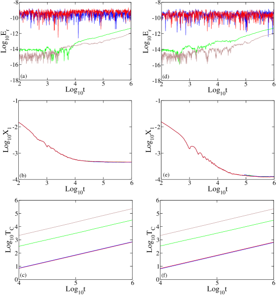
Figure 1: Results for the integration of the equations of motion and the variational equations of the $\alpha$-FPUT Hamiltonian [Eq. (2.1)] for cases (see text for details) $\text{I}_{\text{F}}$ [panels (a), (b) and (c)] and $\text{II}_{\text{F}}$ [panels (d), (e) and (f)] by the SIs $ABA864$ (blue curves) and $SABA_{2}Y6$ (red curves), and the non-symplectic schemes $DOP853$ (green curves) and $TIDES$ (brown curves): the time evolution of, (a) and (d) the relative energy error $E_{r}(t)$ [Eq. (4.3)], (b) and (e) the finite time mLE $X_{1}(t)$ [Eq. (4.1)], (c) and (f) the required CPU time $T_{C}$. All curves in panels (b) and (e), as well as the blue and red curves in panels (c) and (f) overlap.

Table 1: Information on the performance of the numerical schemes used for the integration of the equations of motion and the variational equations of the $\alpha$-FPUT system [Eq. (2.1)] up to the final time $t_{f}=10^{6}$ for case $\text{I}_{\text{F}}$ (see text for details). The order $n$ and the number of steps of each SI, along with the integration time step $\tau$ used to reach a relative energy error $E_{r}\approx 10^{-5}$ and $E_{r}\approx 10^{-9}$, as well as the required CPU time $T_{C}$ in seconds are reported. $\delta$ is the one-step precision of the non-symplectic schemes. Results are presented in increasing $T_{C}$ values. See [95] for practical information on the simulations.

$E_{r}\approx 10^{-5}$					$E_{r}\approx 10^{-9}$
Integrator	$n$	Steps	$\tau$	$T_{C}$	Integrator	$n$	Steps	$\tau$	$T_{C}$
$ABA864$	4	15	$0.6$	88	$SRKN_{14}^{a}$	6	29	$0.45$	160
$ABAH864$	4	17	$0.55$	115	$SRKN_{11}^{b}$	6	23	$0.35$	177
$SABA_{2}Y6$	6	29	$0.575$	167	$s11SABA_{2}6$	6	45	$0.3$	536
$ABA864Y6$	6	43	$0.625$	202	$s19SABA_{2}8$	8	77	$0.45$	594
$s9SABA_{2}6$	6	37	$0.575$	205	$s9ABA82\_6$	6	73	$0.35$	607
$FR4$	4	7	$0.14$	228	$s15SABA_{2}8$	8	61	$0.35$	611
$SBAB_{2}Y6$	6	29	$0.5$	233	$SABA_{2}Y6$	6	29	$0.14$	683
$SABA_{2}K$	4	9	$0.3$	234	$ABA864$	4	15	$0.08$	717
$ABA82Y4$	4	25	$0.375$	240	$s19ABA82\_8$	8	153	$0.65$	773
$s11SABA_{2}6$	6	45	$0.65$	247	$s9SABA_{2}6$	6	37	$0.16$	779
$SABA_{2}Y4$	4	13	$0.18$	265	$ABA864Y6$	6	43	$0.16$	791
$ABA82$	2	5	$0.125$	278	$s15ABA82\_8$	8	121	$0.475$	838
$ABA82Y6$	6	57	$0.675$	283	$ABA82Y6$	6	57	$0.2$	841
$s15SABA_{2}8$	8	61	$0.65$	339	$s11ABA82\_6$	6	89	$0.275$	941
$SABA_{2}$	2	5	$0.07$	347	$SBAB_{2}Y6$	6	29	$0.12$	965
$s19SABA_{2}8$	8	77	$0.775$	356	$ABAH864$	4	17	$0.055$	1013
$SBAB_{2}Y4$	4	13	$0.18$	358	$SABA_{2}Y8\_D$	8	61	$0.175$	1223
$FR4Y6$	6	19	$0.21$	366	$ABA82Y8\_D$	8	121	$0.25$	1575
$s9ABA82\_6$	6	73	$0.575$	369	$SABA_{2}Y4Y6$	6	37	$0.07$	1701
$s11ABA82\_6$	6	89	$0.675$	382	$FR4Y6$	6	19	$0.45$	1787
$SBAB_{2}$	2	5	$0.07$	387	$ABA82Y4Y6$	6	73	$0.125$	1932
$SABA_{2}Y4Y6$	6	37	$0.3$	394	$ABA82Y4$	4	25	$0.0375$	2156
$ABA82Y4Y6$	6	73	$0.525$	405	$SBAB_{2}Y4Y6$	6	37	$0.065$	2239
$SABA_{2}Y8\_D$	8	61	$0.525$	408	$SABA_{2}K$	4	9	$0.03$	2344
$SBAB_{2}K$	4	9	$0.2$	416	$SABA_{2}KY6$	6	$19$	$0.09$	2465
$s19ABA82\_8$	8	153	$1.15$	439	$FR4$	4	7	$0.01$	2597
$SABA_{2}KY6$	6	$19$	0.4	535	$SABA_{2}Y4$	4	13	$0.018$	2654
$SBAB_{2}Y4Y6$	6	37	$0.275$	553	$SBAB_{2}Y4$	4	13	$0.018$	3156
$s15ABA82\_8$	8	121	$0.775$	618	$SABA_{2}Y8\_A$	8	61	$0.06$	3570
$ABA82Y8\_D$	8	121	$0.6$	656	$SBAB_{2}K$	4	9	$0.02$	4167
$SABA_{2}Y8\_A$	8	61	$0.225$	1090	$ABA82Y8\_A$	8	121	$0.07$	5624
$LF$	2	3	$0.018$	1198	$ABA82$	2	5	$0.00125$	27796
$ABA82Y8\_A$	8	121	$0.225$	1749	$DOP853$	8	$\delta=10^{-16}$	0.05	31409
					$SABA_{2}$	2	5	$0.0007$	34595
					$SBAB_{2}$	2	5	$0.0007$	39004
					$LF$	2	3	$0.0002$	95096
					$TIDES$	-	$\delta=10^{-16}$	0.05	$232785$

Table 2: Similar to Table 1 but for case $\text{II}_{\text{F}}$ (see text for details) of the $\alpha$-FPUT system of Eq. (2.1). See [95] for practical information on the simulations

. $E_{r}\approx 10^{-5}$ $E_{r}\approx 10^{-9}$ Integrator $n$ Steps $\tau$ $T_{C}$ Integrator $n$ Steps $\tau$ $T_{C}$ $ABA864$ 4 15 $0.6$ 77 $SRKN_{14}^{a}$ 6 29 $0.475$ 156 $ABAH864$ 4 17 $0.55$ 101 $SRKN_{11}^{b}$ 6 23 $0.35$ 179 $SABA_{2}Y6$ 6 29 $0.575$ 183 $s11SABA_{2}6$ 6 45 $0.3$ 480 $ABA864Y6$ 6 43 $0.625$ 195 $s19SABA_{2}8$ 8 77 $0.45$ 596 $s9SABA_{2}6$ 6 37 $0.575$ 214 $s9ABA82\_6$ 6 73 $0.35$ 611 $ABA82Y4$ 4 25 $0.375$ 224 $ABA864$ 4 15 $0.08$ 613 $s11SABA_{2}6$ 6 45 $0.65$ 227 $s15SABA_{2}8$ 8 61 $0.35$ 618 $FR4$ 4 7 $0.14$ 231 $SABA_{2}Y6$ 6 29 $0.14$ 676 $SABA_{2}K$ 4 9 $0.3$ 241 $s19ABA82\_8$ 8 153 $0.65$ 760 $SBAB_{2}Y6$ 6 29 $0.5$ 255 $ABA864Y6$ 6 43 $0.16$ 811 $SABA_{2}Y4$ 4 13 $0.18$ 270 $s15ABA82\_8$ 8 121 $0.475$ 828 $ABA82$ 2 5 $0.125$ 280 $s9SABA_{2}6$ 6 37 $0.16$ 838 $ABA82Y6$ 6 57 $0.675$ 285 $ABA82Y6$ 6 57 $0.2$ 937 $SBAB_{2}Y4$ 4 13 $0.18$ 316 $SBAB_{2}Y6$ 6 29 $0.12$ 964 $s15SABA_{2}8$ 8 61 $0.65$ 329 $ABAH864$ 4 17 $0.055$ 1023 $s19SABA_{2}8$ 8 77 $0.775$ 336 $s11ABA82\_6$ 6 89 $0.275$ 1062 $FR4Y6$ 6 19 $0.21$ 337 $SABA_{2}Y8\_D$ 8 61 $0.175$ 1230 $SBAB_{2}K$ 4 9 $0.2$ 366 $FR4Y6$ 6 19 $0.45$ 1577 $s9ABA82\_6$ 6 73 $0.575$ 373 $ABA82Y8\_D$ 8 121 $0.25$ 1613 $SABA_{2}$ 2 5 $0.07$ 392 $ABA82Y4Y6$ 6 73 $0.125$ 1702 $SBAB_{2}$ 2 5 $0.07$ 393 $ABA82Y4$ 4 25 $0.0375$ 2113 $ABA82Y4Y6$ 6 73 $0.525$ 398 $SABA_{2}Y4Y6$ 6 37 $0.07$ 2159 $SABA_{2}Y8\_D$ 8 61 $0.525$ 407 $SBAB_{2}Y4Y6$ 6 37 $0.065$ 2310 $s11ABA82\_6$ 6 89 $0.675$ 415 $SABA_{2}KY6$ 6 19 $0.09$ 2380 $s19ABA82\_8$ 8 153 $1.15$ 431 $FR4$ 4 7 $0.01$ 2615 $SABA_{2}Y4Y6$ 6 37 $0.3$ 444 $SABA_{2}K$ 4 9 $0.03$ 2651 $SBAB_{2}Y4Y6$ 6 37 $0.275$ 533 $SABA_{2}Y4$ 4 13 $0.018$ 3016 $SABA_{2}KY6$ 6 19 0.4 540 $SBAB_{2}Y4$ 4 13 $0.018$ 3585 $s15ABA82\_8$ 8 121 $0.775$ 598 $SABA_{2}Y8\_A$ 8 61 $0.06$ 3647 $ABA82Y8\_D$ 8 121 $0.6$ 629 $SBAB_{2}K$ 4 9 $0.02$ 3663 $SABA_{2}Y8\_A$ 8 61 $0.225$ 952 $ABA82Y8\_A$ 8 121 $0.07$ 5691 $LF$ 2 3 $0.018$ 1059 $ABA82$ 2 5 $0.00125$ 31576 $ABA82Y8\_A$ 8 121 $0.225$ 1787 $DOP853$ 8 $\delta=10^{-16}$ 0.05 31709 $SABA_{2}$ 2 5 $0.0007$ 39333 $SBAB_{2}$ 2 5 $0.0007$ 45690 $LF$ 2 3 $0.0002$ 106653 $TIDES$ - $\delta=10^{-16}$ 0.05 $225565$

In Table 1 (Table 2) we present information on the performance of all considered integration schemes for the initial condition of case $\text{I}_{\text{F}}$ (case $\text{II}_{\text{F}}$). From the results of these tables we see that the performance and ranking (according to $T_{C}$) of the integrators do not practically depend on the considered initial condition. It is worth noting that although the non-symplectic schemes manage to achieve better accuracies than the symplectic ones, as their $E_{r}$ values are smaller [Figs. 1(a) and (d)], their implementation is not recommended for the long time evolution of the Hamiltonian system, because they require more CPU time and eventually their $E_{r}$ values will increase above the bounded $E_{r}$ values obtained by the symplectic schemes.

From the results of Tables 1 and 2 we see that the best performing integrators are the fourth order SIs $ABA864$ and $ABAH864$ for $E_{r}\approx 10^{-5}$, and the sixth order SIs $SRKN_{14}^{a}$ and $SRKN_{11}^{b}$ for $E_{r}\approx 10^{-9}$. We note that the best SI for $E_{r}\approx 10^{-5}$, the $ABA864$ scheme, shows a quite good behavior also for $E_{r}\approx 10^{-9}$, making this integrator a valuable numerical tool for dynamical studies of multidimensional Hamiltonian systems. We remark that the eighth order SIs we implemented to achieve the moderate accuracy level $E_{r}\approx 10^{-5}$ exhibited an unstable behavior failing to keep their $E_{r}$ values bounded. A similar behavior was also observed for the two RKN schemes $SRKN_{14}^{a}$, $SRKN_{11}^{b}$ when they were used to obtain $E_{r}\approx 10^{-5}$. Thus, the higher order SIs are best suited for more accurate computations. It is also worth mentioning here that the ranking presented in Tables 1 and 2 is indicative of the performance of the various SIs in the sense that small changes in the implementation (e.g. a change in the last digit of the used $\tau$ value) of integrators with similar behaviors (i.e. similar $T_{C}$ values) could interchange their ranking positions without any noticeable difference in the produced results.

4.2 The 1D disordered discrete nonlinear Schrödinger equation system

We investigate the performance of various integrators of Sec. 3 for the 1D DDNLS system [Eq. (2.2)] by considering a lattice of $N=2^{10}$ sites and integrating two sets of initial conditions (for the same reason we did that for the $\alpha$-FPUT system) up to the final time $t_{f}=10^{6}$. We note that, as was already mentioned in Sec. 3.2.2, this model can be split into three integrable parts, so we will implement the SIs presented in that section. In particular, we consider the following two cases of initial conditions:

• Case $\text{I}_{\text{1D}}$: We initially excite $21$ central sites by attributing to each one of them the same constant norm $s_{j}=(q_{j}^{2}+p_{j}^{2})/2=1$, $1\leq i\leq N$, for $W=3.5$ and $\beta=0.62$. This choice sets the total norm $S_{\text{1D}}=21$. The random disorder parameters $\epsilon_{i}$, $1\leq i\leq N$, are chosen so that the total energy is $H_{1D}\approx 0.0212$.

• Case $\text{II}_{\text{1D}}$: Similar set of initial conditions as in case $\text{I}_{\text{1D}}$ but for $W=3$, $\beta=0.03$. The random disorder parameters $\epsilon_{i}$, $1\leq i\leq N$, are chosen such that $H_{\text{1D}}\approx 3.4444$.

We note that cases $\text{I}_{\text{1D}}$ and $\text{II}_{\text{1D}}$ have been studied in [33] and respectively correspond to the so-called ‘strong chaos’ and ‘weak chaos’ dynamical regimes of this model. As initial normalized deviation vector we use a vector having non-zero coordinates only at the central site of the lattice, while its remaining elements are set to zero.

To evaluate the performance of each implemented integrator we check if the obtained trajectory correctly captures the statistical behavior of the normalized norm density distribution $\zeta_{j}=s_{j}/S_{\text{1D}}$, $1\leq j\leq N$, by computing the distribution’s second moment

$$m_{2}=\sum_{j=1}^{N}\left(j-\overline{j}\right)^{2}\zeta_{j},$$ (4.4)

where $\overline{j}=\sum_{j=1}^{N}j\zeta_{j}$ is the position of the center of the distribution [22, 24, 26, 29, 33, 49, 50]. We also check how accurately the values of the system’s two conserved quantities, i.e. its total energy $H_{\text{1D}}$ [Eq. (2.2)] and norm $S_{\text{1D}}$ [Eq. (2.4)], are kept constant throughout the integration by evaluating the relative energy error $E_{r}(t)$ [similarly to Eq. (4.3)] and the relative norm error

$$S_{r}(t)=\left|\frac{S_{\text{1D}}(t)-S_{\text{1D}}(0)}{S_{\text{1D}}(0)}\right|.$$ (4.5)

In addition, we compute the finite time mLE $X_{1}(t)$ [Eq. (4.1)] in order to characterize the system’s chaoticity and check the proper integration of the variational equations.

We consider several three part split SIs, which we divide into two groups: (i) those integrators with order $n\leq 6$, which we implement in order to achieve an accuracy of $E_{r}\approx 10^{-5}$, and (ii) SIs of order eight used for $E_{r}\approx 10^{-9}$. In addition, the two best performing integrators of the first group are also included in the second group. We do not use higher order SIs for obtaining the accuracy level of $E_{r}\approx 10^{-5}$ because, as was shown in [49] and also discussed in Sec. 4.1, usually this task requires large integration time steps, which typically make the integrators unstable. Moreover, increasing the order $n$ of SIs beyond eight does not improve significantly the performance of the symplectic schemes for high precision ($E_{r}\approx 10^{-9}$) simulations [49]. Therefore we do not consider such integrators in our study.

In Fig. 2 we show the time evolution of the relative energy error $E_{r}(t)$ [panel (a)], the relative norm error $S_{r}(t)$ [panel (b)], the second moment $m_{2}(t)$ [panel (d)], as well as the norm density distribution $\zeta_{j}$ at time $t_{f}\approx 10^{6}$ [panel (c)] for case $\text{I}_{\text{1D}}$ (we note that analogous results were also obtained for case $\text{II}_{\text{1D}}$, although we do not report them here). These results are obtained by the implementation of the the second order SI $\mathcal{ABC}2$ (red curves), the fourth order SI $\mathcal{ABC}Y4$ (blue curves), and the non-symplectic schemes $DOP853$ (green curves) and $TIDES$ (brown curves). The results of Fig. 2 are indicative of the results obtained by the integrators listed in Table 3. The integration time step $\tau$ of the SIs was selected so that the relative energy error is kept at $E_{r}\approx 10^{-5}$ [Fig 2(a)]. From the results of Fig. 2(b) we see that the SIs do not keep $S_{r}$ constant. Nevertheless, our results show that we lose no more than two orders of precision (in the worst case of the $\mathcal{ABC}2$ scheme) during the whole integration. On the other hand, both the relative energy [$E_{r}(t)$] and norm [$S_{r}(t)$] errors of the $TIDES$ and $DOP853$ integrators increase in time, with the $TIDES$ scheme behaving better than the $DOP853$ one. Figs. 2(c) and (d) show that all integrators correctly reproduce the dynamics of the system, as all of them practically produce the same norm density distribution at $t_{f}=10^{6}$ [Fig. 2(c)] and the same evolution of the $m_{2}(t)$ [Fig. 2(d)]. We note that $m_{2}$ increases by following a power law $m_{2}\propto t^{\alpha}$ with $\alpha=1/2$, as was expected for the strong chaos dynamical regime (see for example [33] and references therein).

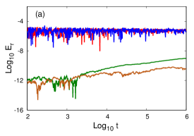
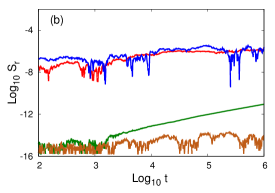
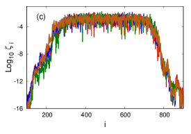
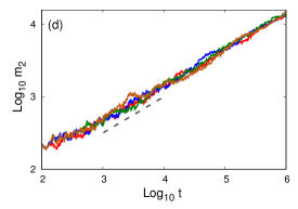
Figure 2: Results for the integration of case $\text{I}_{\text{1D}}$ (see text for details) of the 1D DDNLS model [Eq. (2.2)] by the second order SI $\mathcal{ABC}2$ for $\tau=0.0002$ (red curves), the fourth order SI $\mathcal{ABC}Y4$ for $\tau=0.0125$ (blue curves) and the non-symplectic schemes $DOP853$ (green curves) and $TIDES$ (brown curves): time evolution of (a) the relative energy error $E_{r}(t)$, (b) the relative norm error $S_{r}(t)$ and (d) the second moment $m_{2}(t)$. In (c) the norm density distribution at time $t_{f}=10^{6}$ is shown. The dashed line in (d) guides the eye for slope $1/2$.

Table 3: Data similar to the ones presented in Tables 1 and 2 but for the performance of the numerical schemes used for the integration of the equations of motion and the variational equations of the 1D DDNLS model [Eq. (2.2)] up to the final time $t_{f}=10^{6}$ for case $\text{I}_{\text{1D}}$ (see text for details). See [96] for practical information on the simulations.

$E_{r}\approx 10^{-5}$					$E_{r}\approx 10^{-9}$
Integrator	$n$	Steps	$\tau$	$T_{\text{C}}$	Integrator	$n$	Steps	$\tau$	$T_{\text{C}}$
$s11\mathcal{ABC}6$	$6$	$45$	$0.115$	$3395$	$s19\mathcal{ABC}8$	$8$	$77$	$0.09$	$7242$
$s9\mathcal{ABC}6$	$6$	$37$	$0.095$	$3425$	$s17\mathcal{ABC}8$	$8$	$69$	$0.08$	$7301$
$\mathcal{ABC}Y6\_A$	$6$	$29$	$0.07$	$3720$	$s11\mathcal{ABC}6$	$6$	$45$	$0.025$	$15692$
$SS864S$	$4$	$17$	$0.05$	$6432$	$s9\mathcal{ABC}6$	$6$	$37$	$0.02$	$16098$
$\mathcal{ABC}Y4$	$4$	$13$	$0.0125$	$10317$	$DOP853$	$8$	$\delta=10^{-16}$	$0.05$	$18408$
$\mathcal{ABC}S4Y6$	$6$	$49$	$0.015$	$35417$	$\mathcal{ABC}Y8\_D$	$8$	$61$	$0.002$	$258891$
$\mathcal{ABC}Y4Y6$	$6$	$37$	$0.008$	$40109$	$TIDES$	$-$	$\delta=10^{-16}$	$0.05$	$419958$
$\mathcal{ABC}S4$	$4$	$21$	$0.00085$	$267911$
$\mathcal{ABC}2$	$2$	$5$	$0.0002$	$320581$

In Fig. 3 we show the evolution of the finite time mLE $X_{1}$ [panels (a) and (c)] and the required CPU time $T_{C}$ [panels (b) and (d)] for the integration of the Hamilton equations of motion and the variational equations for cases $\text{I}_{\text{1D}}$ [panels (a) and (b)] and $\text{II}_{\text{1D}}$ [panels (c) and (d)] obtained by using the same integrators of Fig. 2. Again the results obtained by these integrators are practically the same for both sets of initial conditions, reproducing the tendency of the finite time mLE to asymptotically decrease according to the power law $X_{1}(t)\propto t^{\alpha_{L}}$ with $\alpha_{L}\approx-0.3$ (case $\text{I}_{1D}$) and $\alpha_{L}\approx-0.25$ (case $\text{II}_{1D}$), in accordance to the results of [32, 33].

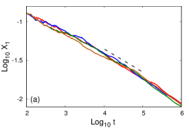
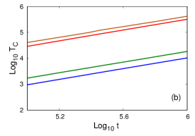
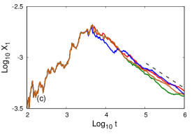
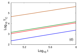
Figure 3: Results obtained by the integration of the variational equations of the 1D DDNLS Hamiltonian [Eq. (2.2)] for the initial conditions described in cases (see text for details) $\text{I}_{\text{1D}}$ [panels (a) and (b)] and $\text{II}_{\text{1D}}$ [panels (c) and (d)]: time evolution of, (a) and (c) the finite time mLE $X_{1}(t)$ [Eq. (4.1)], and (b) and (d) the required CPU time $T_{C}$ in seconds. The dashed lines in (a) and (c) guide the eye for slopes $-0.3$ and $-0.25$ respectively. The integrators and the curve colors are the ones used in Fig. 2.

We now check the efficiency of the used symplectic and non-symplectic methods by comparing the CPU time $T_{C}$ they require to carry out the simulations. These results are reported in Table 3 for case $\text{I}_{\text{1D}}$ and in Table 4 for case $\text{II}_{\text{1D}}$. These tables show that the comparative performance of the integrators does not depend on the chosen initial condition, as the ranking of the schemes is practically the same in both tables. As in the case of the $\alpha$-FPUT model, the $DOP853$ and $TIDES$ integrators required, in general, more CPU time than the SIs, although they produced more accurate results (smaller $E_{r}$ and $S_{r}$ values) at least up to $t_{f}=10^{6}$, with $TIDES$ being more precise. The integrators exhibiting the best performance for $E_{r}\approx 10^{-5}$ are the sixth order SIs $s11\mathcal{ABC}6$ and $s9\mathcal{ABC}6$, while for $E_{r}\approx 10^{-9}$ we have the eighth order SIs $s19\mathcal{ABC}8$ and $s17\mathcal{ABC}8$, with the $s11\mathcal{ABC}6$ scheme performing quite well also in this case.

Table 4: Similar to Table 3 but for case $\text{II}_{\text{1D}}$ (see text for details) of the 1D DDNLS model [Eq. (2.2)]. See [96] for practical information on the simulations.

$E_{r}\approx 10^{-5}$					$E_{r}\approx 10^{-9}$
Integrator	$n$	Steps	$\tau$	$T_{\text{C}}$	Integrator	$n$	Steps	$\tau$	$T_{\text{C}}$
$s11\mathcal{ABC}6$	$6$	$45$	$0.4$	$1132$	$s19\mathcal{ABC}8$	$8$	$77$	$0.3$	$2184$
$s9\mathcal{ABC}6$	$6$	$37$	$0.285$	$1147$	$s17\mathcal{ABC}8$	$8$	$69$	$0.225$	$2632$
$\mathcal{ABC}Y6\_A$	$6$	$29$	$0.2$	$1308$	$s11\mathcal{ABC}6$	$6$	$45$	$0.1$	$4137$
$SS864S$	$4$	$17$	$0.265$	$1365$	$s9\mathcal{ABC}6$	$6$	$37$	$0.075$	$4462$
$\mathcal{ABC}Y4$	$4$	$13$	$0.055$	$2354$	$\mathcal{ABC}Y8\_D$	$8$	$61$	$0.065$	$8528$
$\mathcal{ABC}S4Y6$	$6$	$49$	$0.105$	$4965$	$DOP853$	$8$	$\delta=10^{-16}$	$0.05$	$14998$
$\mathcal{ABC}Y4Y6$	$6$	$37$	$0.04$	$8091$	$TIDES$	$-$	$\delta=10^{-16}$	$0.05$	$420050$
$\mathcal{ABC}S4$	$4$	$21$	$0.02$	$9774$
$\mathcal{ABC}2$	$2$	$5$	$0.0055$	$11700$

4.3 The 2D disordered discrete nonlinear Schrödinger equation system

We now investigate the performance of the integrators used in Sec. 4.2 for the computationally much more difficult case of the 2D DDNLS lattice of Eq. (2.3), as its Hamiltonian function can also be split into three integrable parts. In order to test the performance of the various schemes we consider a lattice with $N\times M=200\times 200$ sites, resulting to a system of $4\times 40\,000=160\,000$ ODEs (equations of motion and variational equations). The numerical integration of this huge number of ODEs is a very demanding computational task. For this reason we integrate this model only up to a final time $t_{f}=10^{5}$, instead of the $t_{f}=10^{6}$ used for the $\alpha$-FPUT and the 1D DDNLS systems. It is worth noting that due to the computational difficulty of the problem very few numerical results for the 2D DDNLS system exist in the literature (e.g. [39, 65]). We consider again two sets of initial conditions:

• Case $\text{I}_{\text{2D}}$: We initially excite $7\times 7$ central sites attributing to each one of them the same norm $s_{i,j}=(q_{i,j}^{2}+p_{i,j}^{2})/2=1/6$ so that the total norm is $S_{\text{2D}}=49/6$, for $W=15$ and $\beta=6$. The disorder parameters $\epsilon_{i,j}$, $1\leq i\leq N$, $1\leq j\leq M$, are chosen so that the initial total energy is $H_{\text{2D}}\approx 1.96$.

• Case $\text{II}_{\text{2D}}$: We initially excite a single central site of the lattice with a total norm $S_{\text{2D}}=1$, i.e. $\zeta_{100,100}=1$, for $W=16$, $\beta=1.25$ and $H_{\text{2D}}=0.625$.

The initial normalized deviation vector considered in our simulations has random non-zero values only at the $7\times 7$ initially excited sites for case $\text{I}_{\text{2D}}$, and only at site $i=100$, $j=100$ for case $\text{II}_{\text{2D}}$. In both cases, all others elements of the vectors are initially set to zero. Both considered cases belong to a Gibbsian regime where the thermalization processes are well defined by Gibbs ensembles [52, 97]. Therefore, we expect a subdiffusive spreading of the initial excitations to take place for both cases, although their initial conditions are significantly different.

As was done in the case of the 1D DDNLS system (Sec. 4.2), in order to evaluate the performance of the used integrators we follow the time evolution of the normalized norm density distribution $\zeta_{i,j}=s_{i,j}/S_{\text{2D}}$, $1\leq i\leq N$, $1\leq j\leq M$ and compute the related second moment $m_{2}$ and participation number $P$

$$m_{2}=\sum_{i=1}^{N}\sum_{j=1}^{M}\left\|(i,j)^{T}-(\overline{i},\overline{j})^{T}\right\|^{2}\zeta_{i,j},\qquad\displaystyle P=\frac{1}{\sum_{i=1}^{N}\sum_{j=1}^{M}\zeta_{i,j}^{2}},$$ (4.6)

where $(\overline{i},\overline{j})^{T}=\sum_{i,j}(i,j)^{T}\zeta_{i,j}$ is the mean position of the norm density distribution. We also evaluate the relative energy [$E_{r}(t)$] and norm [$S_{r}(t)$] errors and compute the finite time mLE $X_{1}(t)$.

In Fig. 4 we present results obtained for case $\text{I}_{\text{2D}}$ by the four best performing SIs (see Table 5), the $s11\mathcal{ABC}6$ (red curves), $s9\mathcal{ABC}6$ (blue curves), $\mathcal{ABC}Y6\_A$ (green curves) and $\mathcal{ABC}Y4$ (brown curves) schemes, along with the $DOP853$ integrator (grey curves). The integration time steps $\tau$ of the SIs were adjusted in order to obtain an accuracy of $E_{r}\approx 10^{-5}$ [Fig. 4(a)], while results for the conservation of the second integral of motion, i.e. the system’s total norm, are shown in Fig. 4(b). We see that for all SIs the $S_{r}$ values increase slowly, remaining always below $S_{r}\approx 10^{-4}$, which indicates a good conservation of the system’s norm. As in the case of the 1D DDNLS system, the $E_{r}$ and $S_{r}$ values obtained by the $DOP853$ integrator increase, although the choice of $\delta=10^{-16}$ again ensures high precision computations.

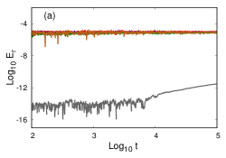
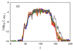
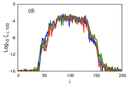
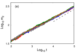
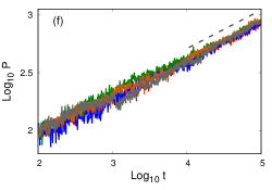
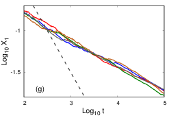
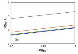
Figure 4: Results for the integration of case $\text{I}_{2D}$ (see text for details) of the 2D DDNLS Hamiltonian [Eq. (2.3)] by the fourth order SI $\mathcal{ABC}Y4$ for $\tau=0.025$, the sixth order SIs $s11\mathcal{ABC}6$ for $\tau=0.125$, $s9\mathcal{ABC}6$ for $\tau=0.105$ and $\mathcal{ABC}Y6\_A$ for $\tau=0.08$, along with the non-symplectic scheme $DOP853$ for $\tau=0.05$ [brown, red, blue, green and grey curves respectively]. Time evolution of (a) $E_{r}(t)$, (b) $S_{r}(t)$, (e) $m_{2}(t)$, (f) $P(t)$, (g) $X_{1}(t)$ and (f) $T_{C}(t)$. In (c) and (d) we plot the norm density distributions along the lines $i=100$ and $j=100$ respectively, at time $t_{f}=10^{5}$. The dashed line in panels (e) and (f) guides the eye for slope $1/3$, while in panel (g) denotes slope -1.

Table 5: Similar to Table 3 but for case $\text{I}_{\text{2D}}$ of the 2D DDNLS model [Eq. (2.3)]. See [96] practical information details on the simulations.

$E_{r}\approx 10^{-5}$					$E_{r}\approx 10^{-9}$
Integrator	$n$	Steps	$\tau$	$T_{\text{C}}$	Integrator	$n$	Steps	$\tau$	$T_{\text{C}}$
$s9\mathcal{ABC}6$	$6$	$45$	$0.105$	$13914$	$s17\mathcal{ABC}8$	$8$	$77$	$0.075$	$36528$
$s11\mathcal{ABC}6$	$6$	$37$	$0.125$	$14000$	$s19\mathcal{ABC}8$	$8$	$69$	$0.08$	$38270$
$\mathcal{ABC}Y6\_A$	$6$	$29$	$0.08$	$15344$	$s9\mathcal{ABC}6$	$6$	$45$	$0.0235$	$65287$
$\mathcal{ABC}Y4$	$4$	$13$	$0.025$	$23030$	$s11\mathcal{ABC}6$	$6$	$37$	$0.0275$	$67314$
$SS864S$	$4$	$17$	$0.085$	$23887$	$\mathcal{ABC}Y8\_D$	$8$	$61$	$0.008$	$140506$
$\mathcal{ABC}S4Y6$	$6$	$49$	$0.03$	$77424$	$DOP853$	$8$	$\delta=10^{-16}$	$0.05$	$218704$
$\mathcal{ABC}Y4Y6$	$6$	$37$	$0.0165$	$87902$
$\mathcal{ABC}S4$	$4$	$21$	$0.0065$	$132713$
$\mathcal{ABC}2$	$2$	$5$	$0.005$	$157694$

The norm density distributions at the final integration time $t_{f}=10^{5}$ along the axis $i=100$ [Fig. 4(c)] and $j=100$ [Fig. 4(d)] obtained by the various integrators practically overlap indicating the ability of all numerical schemes to correctly capture the system’s dynamics, as well as the fact that the initial excitations expand along all directions of the 2D lattice. From Fig. 4(e) [Fig. 4(f)] we see that $m_{2}(t)$ [$P(t)$] is increasing according to the power law $m_{2}=t^{1/3}$ [$P=t^{1/3}$] as expected from the analysis presented in [30], indicating that the 2D lattice is being thermalized. The results of Figs. 4(e) and (f) provide additional numerical evidences that all numerical methods reproduce correctly the dynamics. This is also seen by the similar behavior of the finite time mLE curves in Fig. 4(g). From the results of this figure we see that $X_{1}$ exhibits a tendency to decrease following a completely different decay from the $X_{1}\propto t^{-1}$ power law observed for regular motion. This behavior was also observed for the 2D DKG model [56], as well as for the 1D DKG and DDNLS systems in [32, 33] where a power law $X_{1}(t)\propto t^{\alpha_{L}}$ with $\alpha_{L}\approx-0.25$ and $\alpha_{L}\approx-0.3$ for, respectively, the weak and strong chaos dynamical regimes was established. Further investigations of the behavior of the finite mLE in 2D disordered systems are required in order to determine a potentially global behavior of $X_{1}$, since here and in [56] only some isolated cases were discussed. Such studies will require the statistical analysis of results obtained for many different disorder realizations, parameter sets and initial conditions. Thus, the utilization of efficient and accurate numerical integrators, like the ones presented in this study, will be of utmost importance for the realization of this goal.

From Tables 5 and 6, where the CPU times $T_{C}$ required by the tested integrators are reported, we see that, as in the case of the 1D DDNLS model, the SIs $s11\mathcal{ABC}6$ and $s9\mathcal{ABC}6$ have the best performance for $E_{r}\approx 10^{-5}$ and the SIs $s19\mathcal{ABC}8$ and $s17\mathcal{ABC}8$ for $E_{r}\approx 10^{-9}$.

Table 6: Similar to Table 3 but for case $\text{II}_{\text{2D}}$ of the 2D DDNLS model [Eq. (2.3)]. See [96] for practical information on the simulations.

$E_{r}\approx 10^{-5}$					$E_{r}\approx 10^{-9}$
Integrator	$n$	Steps	$\tau$	$T_{\text{C}}$	Integrator	$n$	Steps	$\tau$	$T_{\text{C}}$
$s11\mathcal{ABC}6$	$6$	$45$	$0.1515$	$11443$	$s19\mathcal{ABC}8$	$8$	$77$	$0.135$	$20952$
$s9\mathcal{ABC}6$	$6$	$37$	$0.11$	$13408$	$s17\mathcal{ABC}8$	$8$	$69$	$0.0875$	$28966$
$\mathcal{ABC}Y6\_A$	$6$	$29$	$0.0775$	$14607$	$s11\mathcal{ABC}6$	$6$	$45$	$0.0335$	$50301$
$SS864S$	$4$	$17$	$0.0915$	$15564$	$s9\mathcal{ABC}6$	$6$	$37$	$0.024$	$58187$
$\mathcal{ABC}Y4$	$4$	$13$	$0.0215$	$25898$	$\mathcal{ABC}Y8\_D$	$8$	$61$	$0.009$	$150045$
$\mathcal{ABC}S4Y6$	$6$	$49$	$0.035$	$64423$	$DOP853$	$8$	$\delta=10^{-16}$	$0.05$	$166145$
$\mathcal{ABC}Y4Y6$	$6$	$37$	$0.01375$	$102580$
$\mathcal{ABC}S4$	$4$	$21$	$0.005$	$185615$
$\mathcal{ABC}2$	$2$	$5$	$0.00155$	$198534$

5 Conclusions

In this work we carried out a methodical and detailed analysis of the performance of several symplectic and non-symplectic integrators, which were used to integrate the equations of motion and the variational equations of some important many-body classical Hamiltonian systems in one and two spatial dimensions: the $\alpha$-FPUT chain, as well as the 1D and 2D DDNLS models. In the case of the $\alpha$-FPUT system we used two part split SIs, while for the integration of the DDNLS models we implemented several three part split SIs. In order to evaluate the efficiency of all these integrators we evolved in time different sets of initial conditions and evaluated quantities related to (a) the dynamical evolution of the studied systems (e.g. the second moment of norm density distributions for the DDNLS models), (b) the quantification of the systems’ chaotic behavior (i.e. the finite time mLE), and (c) the accurate computation of the systems’ integrals of motion (relative energy and norm errors), along with the CPU times needed to perform the simulations.

For the $\alpha$-FPUT system several two part split SIs showed very good performances, among which we mention the $ABA864$ and $ABAH864$ SIs of order four to be the best schemes for moderate energy accuracies ($E_{r}\approx 10^{-5}$), while the $SRKN^{a}_{14}$ and $SRKN^{b}_{11}$ SIs of order six were the best integration schemes for higher accuracies ($E_{r}\approx 10^{-9}$). In particular, the $ABA864$ scheme appears to be an efficient, general choice as it showed a quite good behavior also for $E_{r}\approx 10^{-9}$. Concerning the 1D and the 2D DDNLS models our simulations showed that the SIs $s9\mathcal{ABC}6$ and $s11\mathcal{ABC}6$ (order six), along with the SIs $s17\mathcal{ABC}8$ and $s19\mathcal{ABC}8$ (order eight) are the best integrators for moderate ($E_{r}\approx 10^{-5}$) and high ($E_{r}\approx 10^{-9}$) accuracy levels respectively.

The $DOP853$ and $TIDES$ non-symplectic integrators required, in general, much longer CPU times to carry out the simulations, although they produced more accurate results (i.e smaller $E_{r}$ and $S_{r}$ values) than the symplectic schemes. Apart from the drawback of the high CPU times, the fact that $E_{r}$ (and $S_{r}$) values exhibit a constant increase in time signifies that such schemes should not be preferred over SIs when very long time simulations are needed.

It is worth noting that two part split SIs of order six and higher often do now not produce reliable results for relative low energy accuracies like $E_{r}\approx 10^{-5}$ for the $\alpha$-FPUT system (similar behaviors were reported in [56] for the DKG model). This happens because the required integration time step $\tau$ needed to keep the relative energy error at $E_{r}\approx 10^{-5}$ is typically large, resulting to an unstable behavior of the integrator i.e. the produced $E_{r}$ values do not remain bounded. Thus, SIs of order $n\geq 6$ are more suitable for calculations that require higher accuracies (e.g. $E_{r}\approx 10^{-9}$ or lower).

We note that we presented here a detailed comparison of the performance of several two and three part split SIs for the integration of the variational equations through the tangent map method and consequently for the computation of a chaos indicator (the mLE), generalizing, and completing in some sense, some sporadic previous investigation of the subject [56, 58, 59, 60], which were only focused on two part split SIs.

We hope that the clear description of the construction of several two and three part split SIs in Sec. 3, along with the explicit presentation in the Appendix of the related differential operators for many commonly used classical, many-body Hamiltonians will be useful to researchers working on lattice dynamics. The numerical techniques presented here can be used for the computation of several chaos indicators, apart from the mLE (e.g. the SALI and the GALI methods [98]) and for the dynamical study of various lattice models, like for example of arrays of Josephson junctions in regimes of weak non-integrability [53], granular chains [99] and DNA models [91], to name a few.

Appendix

Appendix A Explicit forms of tangent map method operators

We present here the exact expressions of the operators needed by the various SIs we implemented in our study to simultaneously solve the Hamilton equations of motion and the variational equations, or in order words to solve the system of Eq. (3.7)

$$\dot{\boldsymbol{X}}=(\dot{\boldsymbol{x}}(t),\dot{\delta\boldsymbol{x}}(t))=\boldsymbol{f}(\boldsymbol{X})=\begin{bmatrix}\boldsymbol{J}_{2N}\cdot\boldsymbol{D}_{H}(\boldsymbol{x}(t))\\ \big{[}\boldsymbol{J}_{2N}\cdot\boldsymbol{D}_{H}^{2}(\boldsymbol{x}(t))\big{]}\cdot\delta\boldsymbol{x}(t)\end{bmatrix}.$$ (A.1)

A.1 The $\alpha$-Fermi-Pasta-Ulam-Tsingou model

The Hamiltonian of the $\alpha$-FPUT chain [Eq. (2.1)] can be split into two integrable parts as

$$A\left(\boldsymbol{p}\right)=\sum_{i=0}^{N}\ \frac{p_{i}^{2}}{2},\qquad B\left(\boldsymbol{q}\right)=\sum_{i=0}^{N}\ \frac{1}{2}(q_{i+1}-q_{i})^{2}+\frac{\alpha}{3}(q_{i+1}-q_{i})^{3}.$$ (A.2)

As we have already stated, the split into two integrable parts is not necessarily unique. In this particular case another possible choice of integrable splits for the $\alpha$-FPUT chain is to group together the quadratic terms of the Hamiltonian [i.e. $A({\bf p},{\bf q})=\sum_{i=0}^{N}\ \frac{p_{i}^{2}}{2}+\frac{1}{2}(q_{i+1}-q_{i})^{2}$] and keep separately the nonlinear terms [i.e. $B({\bf q})=\sum_{i=0}^{N}\ \frac{\alpha}{3}(q_{i+1}-q_{i})^{3}$]. The set of equations of motion and variational equations for the Hamiltonian function $A\left(\boldsymbol{p}\right)$ is

$$\frac{d\boldsymbol{X}}{dt}=L_{AZ}\boldsymbol{X}\colon\begin{cases}\dot{q}_{i}&=p_{i}\\ \dot{p}_{i}&=0\\ \dot{\delta q}_{i}&=\delta p_{i}\\ \dot{\delta p}_{i}&=0\end{cases},\qquad\text{for}\qquad 1\leq i\leq N,$$ (A.3)

and the corresponding operator $e^{\tau L_{AZ}}$, which propagates the values of $q_{i}$, $p_{i}$, $\delta q_{i}$ and $\delta p_{i}$ for $\tau$ time units in the future, obtaining $q_{i}^{\prime}$, $p_{i}^{\prime}$, $\delta q_{i}^{\prime}$ and $\delta p_{i}^{\prime}$, takes the form

$$e^{\tau L_{AZ}}\colon\begin{cases}q_{i}^{\prime}&=q_{i}+\tau p_{i}\\ p_{i}^{\prime}&=p_{i}\\ \delta q_{i}^{\prime}&=\delta q_{i}+\tau\delta p_{i}\\ \delta p_{i}^{\prime}&=\delta p_{i}\end{cases},\qquad\text{for}\qquad 1\leq i\leq N.$$ (A.4)

In a similar way for the $B\left(\boldsymbol{q}\right)$ Hamiltonian of Eq. (A.2) we get

$$\frac{d\boldsymbol{X}}{dt}=L_{BZ}\boldsymbol{X}\colon\begin{cases}\dot{q}_{i}&=0\\ \dot{p}_{i}&=(q_{i+1}+q_{i-1}-2q_{i})+\alpha\big{[}(q_{i+1}-q_{i})^{2}-(q_{i}-q_{i-1})^{2}\big{]}\\ \dot{\delta q}_{i}&=0\\ \dot{\delta p}_{i}&=[2\alpha(q_{i-1}-q_{i+1})-2]\delta q_{i}+[1+2\alpha(q_{i+1}-q_{i})]\delta q_{i+1}+[1+2\alpha(q_{i}-q_{i-1})]\delta q_{i-1}\end{cases},$$ (A.5)

and

$$e^{\tau L_{BZ}}\colon\begin{cases}q_{i}^{\prime}&=q_{i}\\ p_{i}^{\prime}&=p_{i}+\tau\big{\{}(q_{i+1}+q_{i-1}-2q_{i})+\alpha\big{[}(q_{i+1}-q_{i})^{2}-(q_{i}-q_{i-1})^{2}\big{]}\big{\}}\\ \delta q_{i}^{\prime}&=\delta q_{i}\\ \delta p_{i}^{\prime}&=\delta p_{i}+\tau\big{\{}[2\alpha(q_{i-1}-q_{i+1})-2]\delta q_{i}+[1+2\alpha(q_{i+1}-q_{i})]\delta q_{i+1}+[1+2\alpha(q_{i}-q_{i-1})]\delta q_{i-1}\big{\}}\end{cases}.$$ (A.6)

According to Eq. (3.26) the accuracy of the $SABA_{n}$ and $SBAB_{n}$ integrators can be improved by using a corrector Hamiltonian $K$ [55]. In the case of a separable Hamiltonian $H(\boldsymbol{q},\boldsymbol{p})=A(\boldsymbol{p})+B(\boldsymbol{q})$ with $A\left(\boldsymbol{p}\right)=\sum_{i=1}^{N}p_{i}^{2}/2$, the corrector $K$ becomes

$$K(\boldsymbol{q})=\{B\{B,A\}\}=\sum_{i=1}^{N}\ \left(\frac{\partial B}{\partial q_{i}}\right)^{2}.$$ (A.7)

For the $\alpha$-FPUT chain, the corrector Hamiltonian $K$ is

$$\begin{split}K(\boldsymbol{q})&=\sum_{i=1}^{N}\Big{[}\big{(}2q_{i}-q_{i+1}-q_{i-1}\big{)}\big{(}1+\alpha(q_{i+1}-q_{i-1})\big{)}\Big{]}^{2}\ .\\ \end{split}$$ (A.8)

As the equations of motion and variational equations associated to the corrector Hamiltonian $K$ are cumbersome, we report here only the form of the operator $e^{\tau L_{KZ}}$

$$e^{\tau L_{KZ}}\colon\begin{cases}q_{i}^{\prime}&=q_{i}\\ p_{i}^{\prime}&=p_{i}+2\tau\Big{\{}2\big{(}q_{i+1}+q_{i-1}-2q_{i}\big{)}\big{[}1+\alpha\big{(}q_{i+1}-q_{i-1}\big{)}\big{]}^{2}\\ &-\big{(}q_{i+2}+q_{i}-2q_{i+1}\big{)}\big{[}1+\alpha\big{(}q_{i+2}-q_{i}\big{)}\big{]}\big{[}1-2\alpha\big{(}q_{i}-q_{i+1}\big{)}\big{]}\\ &-\big{(}q_{i-2}+q_{i}-2q_{i-1}\big{)}\big{[}1+\alpha\big{(}q_{i}-q_{i-2}\big{)}\big{]}\big{[}1-2\alpha\big{(}q_{i-1}-q_{i}\big{)}\big{]}\Big{\}}\\ \delta q_{i}^{\prime}&=\delta q_{i}\\ \delta p_{i}^{\prime}&=\delta p_{i}+\tau\big{\{}\gamma_{i}\delta q_{i}+\gamma_{i+1}\delta q_{i+1}+\gamma_{i+2}\delta q_{i+2}+\gamma_{i-1}\delta q_{i-1}+\gamma_{i-2}\delta q_{i-2}\big{\}}\end{cases},$$ (A.9)

where

$$\begin{split}\gamma_{i}&=-2\Big{\{}4\big{[}1+\alpha\big{(}q_{i+1}-q_{i-1}\big{)}\big{]}^{2}\\ &\qquad\quad+\big{[}1+\alpha\big{(}q_{i+2}-q_{i}\big{)}\big{]}\big{[}1-2\alpha\big{(}q_{i}-q_{i+1}\big{)}\big{]}\\ &\qquad\quad+\big{[}1+\alpha\big{(}q_{i}-q_{i-2}\big{)}\big{]}\big{[}1-2\alpha\big{(}q_{i-1}-q_{i}\big{)}\big{]}\\ &\qquad\quad+\alpha\big{(}2q_{i+1}-q_{i+2}-q_{i}\big{)}\big{[}3-4\alpha q_{i}+2\alpha q_{i+1}+2\alpha q_{i+2}\big{]}\\ &\qquad\quad-\alpha\big{(}2q_{i-1}-q_{i-2}-q_{i}\big{)}\big{[}3+4\alpha q_{i}-2\alpha q_{i-1}-2\alpha q_{i-2}\big{]}\Big{\}}\\ \gamma_{i+1}&=4\Big{\{}\big{[}1+\alpha\big{(}q_{i+1}-q_{i-1}\big{)}\big{]}\big{[}1-\alpha\big{(}4q_{i}-3q_{i+1}-q_{i-1}\big{)}\big{]}\\ &\qquad\quad+\big{[}1+\alpha\big{(}q_{i+2}-q_{i}\big{)}\big{]}\Big{[}1+\alpha\big{(}4q_{i+1}-3q_{i}-q_{i+2}\big{)}\Big{]}\Big{\}}\\ \gamma_{i-1}&=4\Big{\{}\big{[}1+\alpha\big{(}q_{i+1}-q_{i-1}\big{)}\big{]}\big{[}1+\alpha\big{(}4q_{i}-3q_{i-1}-q_{i+1}\big{)}\big{]}\\ &\qquad\quad+\big{[}1+\alpha\big{(}q_{i}-q_{i-2}\big{)}\big{]}\Big{[}1-\alpha\big{(}4q_{i-1}-3q_{i}-q_{i-2}\big{)}\Big{]}\Big{\}}\\ \gamma_{i+2}&=2\big{[}1-2\alpha\big{(}q_{i}-q_{i+1}\big{)}\big{]}\big{[}2\alpha\big{(}q_{i+1}-q_{i+2}\big{)}-1\big{]}\\ \gamma_{i-2}&=2\big{[}1-2\alpha\big{(}q_{i-1}-q_{i}\big{)}\big{]}\big{[}2\alpha\big{(}q_{i-2}-q_{i-1}\big{)}-1\big{]}\end{split}.$$ (A.10)

We did not specify the range of index $i$ in Eqs. (A.5), (A.6) and (A.9) intentionally, because it depends on the type of the used boundary conditions. In particular, the expression of Eqs. (A.5), (A.6) and (A.9) are accurate for the case of periodic boundary conditions, i.e. $q_{0}=q_{N}$, $p_{0}=p_{N}$, $\delta q_{0}=\delta q_{N}$, $\delta p_{0}=\delta p_{N}$, $q_{N+1}=q_{1}$, $p_{N+1}=p_{1}$, $\delta q_{N+1}=\delta q_{1}$, $\delta p_{N+1}=\delta p_{1}$. In the case of fixed boundary conditions we considered in our numerical simulations, some adjustments have to be done for the $i=1$ and $i=N$ equations, like the ones reported in the Appendix of [56] where the operators for the 1D and 2D DKG models were reported (with the exception of the corrector term).

For completeness sake in Sec. A.4 we provide the explicit expression of the $e^{\tau L_{BZ}}$ and $e^{\tau L_{KZ}}$ operators for some commonly used Hamiltonians, which can be split into two integrable parts, one of which is the usual kinetic energy $A\left(\boldsymbol{p}\right)=\sum_{i=1}^{N}p_{i}^{2}/2$.

A.2 The 1D disordered discrete nonlinear Schrödinger equation

Here we focus on the 1D DDNLS system, whose Hamiltonian [Eq. (2.2)] can be split into three integrable parts as

$$\begin{split}\mathcal{A}_{1}=\sum_{i=1}^{N}\frac{\epsilon_{i}}{2}(q_{i}^{2}+p_{i}^{2})+\frac{\beta}{8}(q_{i}^{2}+p_{i}^{2})^{2},\qquad\mathcal{B}_{1}=-\sum_{i=1}^{N}p_{i+1}p_{i}\ ,\qquad\mathcal{C}_{1}=-\sum_{i=1}^{N}q_{i+1}q_{i}\end{split}.$$ (A.11)

The set of equations of motion and variational equations associated with the Hamiltonian function $\mathcal{A}_{1}$ is

$$\frac{d\boldsymbol{X}}{dt}=L_{\mathcal{A}_{1}Z}\boldsymbol{X}\colon\begin{cases}\dot{q}_{i}&=p_{i}\theta_{i}\\ \dot{p}_{i}&=-q_{i}\theta_{i},\\ \dot{\delta q}_{i}&=\left[\theta_{i}+\beta p_{i}^{2}\right]\delta p_{i}+\beta q_{i}p_{i}\delta q_{i}\\ \dot{\delta p}_{i}&=-\left[\theta_{i}+\beta q_{i}^{2}\right]\delta q_{i}-\beta q_{i}p_{i}\delta p_{i}\end{cases},\qquad\text{for}\qquad 1\leq i\leq N$$ (A.12)

with $\theta_{i}=\epsilon_{i}+\beta(q_{i}^{2}+p_{i}^{2})/2$ for $i=1,2,\ldots,N$ being constants of the motion. The corresponding operator $e^{\tau L_{\mathcal{A}_{1}Z}}$ takes the form

$$e^{\tau L_{\mathcal{A}_{1}Z}}\colon\begin{cases}q_{i}^{\prime}&=q_{i}\cos(\tau\alpha_{i})+p_{i}\sin(\tau\alpha_{i})\\ p_{i}^{\prime}&=p_{i}\cos(\tau\alpha_{i})-q_{i}\sin(\tau\alpha_{i})\\ \delta q_{i}^{\prime}&=\frac{q_{i}\cos(\tau\alpha_{i})+p_{i}\sin(\tau\alpha_{i})}{2J_{i}}\delta J_{i}+\left(p_{i}\cos(\tau\alpha_{i})-q_{i}\sin(\tau\alpha_{i})\right)\left(\beta\delta J_{i}\tau+\delta\theta_{i}\right)\\ \delta p_{i}^{\prime}&=\frac{p_{i}\cos(\tau\alpha_{i})-q_{i}\sin(\tau\alpha_{i})}{2J_{i}}\delta J_{i}-\left(q_{i}\cos(\tau\alpha_{i})+p_{i}\sin(\tau\alpha_{i})\right)\left(\beta\delta J_{i}\tau+\delta\theta_{i}\right)\end{cases},\quad\text{for}\quad 1\leq i\leq N$$ (A.13)

with $J_{i}\neq 0$ and

$$\begin{split}J_{i}=\frac{1}{2}(q_{i}^{2}+p_{i}^{2})\ ,\qquad\alpha_{i}=\epsilon_{i}+\beta J_{i}\ ,\qquad\delta J_{i}=q_{i}\delta q_{i}+p_{i}\delta p_{i}\ ,\qquad\delta\theta_{i}=\frac{p_{i}}{2J_{i}}\delta q_{i}-\frac{q_{i}}{2J_{i}}\delta p_{i}\end{split}.$$ (A.14)

We note that in the special case of $J_{i}=0$ we have $q_{i}=p_{i}=0$. Then the system of Eq. (A.12) takes the simple form $\dot{q_{i}}=0$, $\dot{p_{i}}=0$, $\dot{\delta q}_{i}=\epsilon_{i}\delta p_{i}$, $\dot{\delta p}_{i}=-\epsilon_{i}\delta q_{i}$, leading to $q_{i}^{\prime}=q_{i}$, $p_{i}^{\prime}=p_{i}$, $\delta q_{i}^{\prime}=\delta q_{i}\cos(\epsilon_{i}\tau)+\delta p_{i}\sin(\epsilon_{i}\tau)$, $\delta p_{i}^{\prime}=\delta p_{i}\cos(\epsilon_{i}\tau)-\delta q_{i}\sin(\epsilon_{i}\tau)$.

The set of equations of motion and variational equations associated to the intermediate Hamiltonian functions $\mathcal{B}_{1}$ and $\mathcal{C}_{1}$ are respectively

$$\begin{split}\frac{d\boldsymbol{X}}{dt}=L_{\mathcal{B}_{1}Z}\boldsymbol{X}:\left\{\begin{array}[]{rl}\dot{q}_{i}&=-p_{i-1}-p_{i+1}\\ \dot{p}_{i}&=0\\ \dot{\delta q}_{i}&=-\delta p_{i-1}-\delta p_{i+1}\\ \dot{\delta p}_{i}&=0\end{array}\right.,\quad\text{and}\quad\frac{d\boldsymbol{X}}{dt}=L_{\mathcal{C}_{1}Z}\boldsymbol{X}:\left\{\begin{array}[]{rl}\dot{q_{i}}&=0\\ \dot{p_{i}}&=q_{i-1}+q_{i+1}\\ \dot{\delta q_{i}}&=0\\ \dot{\delta p_{i}}&=\delta q_{i-1}+\delta q_{i+1}\end{array}\right..\end{split}$$ (A.15)

These yield to the operators $e^{L_{\mathcal{B}_{1}Z}}$ and $e^{L_{\mathcal{C}_{1}Z}}$ given by

$$\begin{split}e^{\tau L_{\mathcal{B}_{1}Z}}\colon\left\{\begin{array}[]{rl}q_{i}^{\prime}&=q_{i}-\tau(p_{i-1}+p_{i+1})\\ p_{i}^{\prime}&=p_{i}\\ \delta q_{i}^{\prime}&=\delta q_{i}-\tau(\delta p_{i-1}+\delta p_{i+1})\\ \delta p_{i}^{\prime}&=\delta p_{i}\end{array}\right.\qquad\qquad e^{\tau L_{\mathcal{C}_{1}Z}}\colon\left\{\begin{array}[]{rl}q_{i}^{\prime}&=q_{i}\\ p_{i}^{\prime}&=p_{i}+\tau(q_{i-1}+q_{i+1})\\ \delta q_{i}^{\prime}&=\delta q_{i}\\ \delta p_{i}^{\prime}&=\delta p_{i}+\tau(\delta q_{i-1}+\delta q_{i+1})\\ \end{array}\right..\end{split}$$ (A.16)

As in the case of the $\alpha$-FPUT model, Eqs. (A.15) and (A.16) correspond to the case of periodic boundary conditions and adjustments similar to the ones presented in the Appendix of [56] for the 1D DKG model, should be implemented when fixed boundary conditions are imposed.

A.3 The 2D disordered discrete Nonlinear Schrödinger equation

The Hamiltonian $H_{\text{2D}}$ of Eq. (2.3) can be split into three integrable parts $\mathcal{A}_{2}$, $\mathcal{B}_{2}$ and $\mathcal{C}_{2}$ as

$$\begin{split}\mathcal{A}_{2}=\sum_{i=1}^{N}\sum_{j=1}^{M}\frac{\epsilon_{i,j}}{2}\left[q_{i,j}^{2}+p_{i,j}^{2}\right]+\frac{\beta}{8}\left[q_{i,j}^{2}+p_{i,j}^{2}\right]^{2},\qquad\quad\mathcal{B}_{2}&=\sum_{i=1}^{N}\sum_{j=1}^{M}-p_{i,j+1}p_{i,j}-p_{i+1,j}p_{i,j},\\ \mathcal{C}_{2}&=\sum_{i=1}^{N}\sum_{j=1}^{M}-q_{i,j+1}q_{i,j}-q_{i+1,j}q_{i,j}.\end{split}$$ (A.17)

The equations of motion and the variational equations associated with the $\mathcal{A}_{2}$ Hamiltonian are

$$\begin{split}\frac{d\boldsymbol{X}}{dt}=L_{\mathcal{A}_{2}Z}\boldsymbol{X}&:\left\{\begin{array}[]{rl}\dot{q}_{i,j}&=p_{i,j}\theta_{i,j}\\ \dot{p}_{i,j}&=-q_{i,j}\theta_{i,j},\\ \dot{\delta q}_{i,j}&=\left[\theta_{i,j}+\beta p_{i,j}^{2}\right]\delta p_{i,j}+\beta q_{i,j}p_{i,j}\delta q_{i,j}\\ \dot{\delta p}_{i,j}&=-\left[\theta_{i,j}+\beta q_{i,j}^{2}\right]\delta q_{i,j}-\beta q_{i,j}p_{i,j}\delta p_{i,j}\end{array}\right.,\\ \end{split}$$ (A.18)

for $1\leq i\leq N$, $1\leq j\leq M$, with $\theta_{i,j}=\epsilon_{i,j}+\beta(q_{i,j}^{2}+p_{i,j}^{2})/2$ being constants of motion for the Hamiltonian $\mathcal{A}_{2}$. Then, the operator $e^{\tau L_{\mathcal{A}_{2}Z}}$ is

$$\begin{split}e^{\tau L_{\mathcal{A}_{2}Z}}:\left\{\begin{array}[]{rl}q_{i,j}^{\prime}&=q_{i,j}\cos(\tau\alpha_{i,j})+p_{i,j}\sin(\tau\alpha_{i,j})\\ p_{i,j}^{\prime}&=p_{i,j}\cos(\tau\alpha_{i,j})-q_{i,j}\sin(\tau\alpha_{i,j})\\ \delta q_{i,j}^{\prime}&=\frac{q_{i,j}\cos(\tau\alpha_{i,j})+p_{i,j}\sin(\tau\alpha_{i,j})}{2J_{i,j}}\delta J_{i,j}+\left(p_{i,j}\cos(\tau\alpha_{i,j})-q_{i,j}\sin(\tau\alpha_{i,j})\right)\left(\beta\delta J_{i,j}\tau+\delta\theta_{i,j}\right)\\ \delta p_{i,j}^{\prime}&=\frac{p_{i,j}\cos(\tau\alpha_{i,j})-q_{i,j}\sin(\tau\alpha_{i,j})}{2J_{i,j}}\delta J_{i,j}-\left(q_{i,j}\cos(\tau\alpha_{i,j})+p_{i,j}\sin(\tau\alpha_{i,j})\right)\left(\beta\delta J_{i,j}\tau+\delta\theta_{i,j}\right)\end{array}\right.\end{split}$$ (A.19)

with $J_{i,j}\neq 0$ and

$$\begin{split}&\qquad\quad J_{i,j}=\frac{1}{2}(q_{i,j}^{2}+p_{i,j}^{2})\ ,\qquad\alpha_{i,j}=\epsilon_{i,j}+\beta J_{i,j}\ ,\\ &\delta J_{i,j}=q_{i,j}\delta q_{i,j}+p_{i,j}\delta p_{i,j}\ ,\qquad\delta\theta_{i,j}=\frac{p_{i,j}}{2J_{i,j}}\delta q_{i,j}-\frac{q_{i,j}}{2J_{i,j}}\delta p_{i,j}\end{split}.$$ (A.20)

Again, in the special case of $J_{i,j}=0$, the system of Eq. (A.18) takes the form $\dot{q_{i,j}}=0$, $\dot{p_{i,j}}=0$, $\dot{\delta q}_{i,j}=\epsilon_{i,j}\delta p_{i,j}$, $\dot{\delta p}_{i,j}=-\epsilon_{i,j}\delta q_{i,j}$, leading to $q_{i,j}^{\prime}=q_{i,j}$, $p_{i,j}^{\prime}=p_{i,j}$, $\delta q_{i,j}^{\prime}=\delta q_{i,j}\cos(\epsilon_{i,j}\tau)+\delta p_{i,j}\sin(\epsilon_{i,j}\tau)$, $\delta p_{i,j}^{\prime}=\delta p_{i,j}\cos(\epsilon_{i,j}\tau)-\delta q_{i,j}\sin(\epsilon_{i,j}\tau)$.

The equations of motion and the variational equations for Hamiltonians $\mathcal{B}_{2}$ and $\mathcal{C}_{2}$ are

$$\begin{split}\frac{d\boldsymbol{X}}{dt}=L_{\mathcal{B}_{2}Z}\boldsymbol{X}&:\left\{\begin{array}[]{rl}\dot{q}_{i,j}&=-p_{i-1,j}-p_{i,j-1}-p_{i,j+1}-p_{i+1,j}\\ \dot{p}_{i,j}&=0\\ \dot{\delta q}_{i,j}&=-\delta p_{i-1,j}-\delta p_{i,j-1}-\delta p_{i,j+1}-\delta p_{i+1,j}\\ \dot{\delta p}_{i,j}&=0\end{array}\right.\end{split},$$ (A.21)

and

$$\begin{split}\frac{d\boldsymbol{X}}{dt}=L_{\mathcal{C}_{2}Z}\boldsymbol{X}&:\left\{\begin{array}[]{rl}\dot{p}_{i,j}&=q_{i-1,j}+q_{i,j-1}+q_{i,j+1}+q_{i+1,j}\\ \dot{q}_{i,j}&=0\\ \dot{\delta p}_{i,j}&=\delta q_{i-1,j}+\delta q_{i,j-1}+\delta q_{i,j+1}+\delta q_{i+1,j}\\ \dot{\delta q}_{i,j}&=0\\ \end{array}\right.\end{split},$$ (A.22)

while the corresponding operators $e^{L_{\mathcal{B}_{2}Z}}$ and $e^{L_{\mathcal{C}_{2}Z}}$ are respectively

$$\begin{split}e^{\tau L_{\mathcal{B}_{2}Z}}&:\left\{\begin{array}[]{rl}q_{i,j}^{\prime}&=q_{i,j}-\tau\left(p_{i-1,j}+p_{i,j-1}+p_{i,j+1}+p_{i+1,j}\right)\\ p_{i,j}^{\prime}&=p_{i,j}\\ \delta q_{i,j}^{\prime}&=\delta q_{i,j}-\tau\left(\delta p_{i-1,j}+\delta p_{i,j-1}+\delta p_{i,j+1}+\delta p_{i+1,j}\right)\\ \delta p_{i,j}^{\prime}&=\delta p_{i,j}\\ \end{array}\right.\\ \end{split},$$ (A.23)

and

$$\begin{split}e^{\tau L_{\mathcal{C}_{2}Z}}&:\left\{\begin{array}[]{rl}q_{i,j}^{\prime}&=q_{i,j}\\ p_{i,j}^{\prime}&=p_{i,j}+\tau\left(q_{i-1,j}+q_{i,j-1}+q_{i,j+1}+q_{i+1,j}\right)\\ \delta q_{i,j}^{\prime}&=\delta q_{i,j}\\ \delta p_{i,j}^{\prime}&=\delta p_{i,j}+\tau\left(\delta q_{i-1,j}+\delta q_{i,j-1}+\delta q_{i,j+1}+\delta q_{i+1,j}\right)\end{array}\right..\end{split}$$ (A.24)

Here again Eqs. (A.21), (A.22), (A.23) and (A.24) correspond to the case of periodic boundary conditions. For fixed boundary conditions adjustments similar to the ones report in the Appendix of [56] for the 2D DKG lattice should be performed.

A.4 Other Hamiltonian models which can be split into two integrable parts

We present here the exact expressions of the tangent map operators needed in symplectic integration schemes which can be used to numerically integrate some important models in the field of classical many-body systems: the $\beta$-FPUT chain, the KG model, and the classical XY model (a JJC system) [53, 100, 101, 102]. Similarly to the $\alpha$-FPUT chain of Eq. (2.1), the Hamiltonians $H(\boldsymbol{q},\boldsymbol{p})$ of each of these systems can be split as

$$H(\boldsymbol{q},\boldsymbol{p})=A(\boldsymbol{p})+B(\boldsymbol{q})=\sum_{i=1}^{N}\frac{p_{i}^{2}}{2}+B\left(\boldsymbol{q}\right)$$ (A.25)

with appropriately defined potential terms $B\left(\boldsymbol{q}\right)$:

$$\text{$\beta$-FPUT:}\ \qquad B_{\beta}\left(\boldsymbol{q}\right) =\sum_{i=0}^{N}\frac{1}{2}(q_{i+1}-q_{i})^{2}+\frac{\beta}{4}(q_{i+1}-q_{i})^{4},$$ (A.26)

$$\text{KG:}\ \qquad B_{K}\left(\boldsymbol{q}\right) =\sum_{i=1}^{N}\frac{q_{i}^{2}}{2}+\frac{q_{i}^{4}}{4}+\frac{k}{2}(q_{i+1}-q_{i})^{2},$$ (A.27)

$$\text{JJC:}\ \qquad B_{R}\left(\boldsymbol{q}\right) =\sum_{i=1}^{N}E_{J}\left[1-\cos(q_{i+1}-q_{i})\right],$$ (A.28)

where $\beta$, $k$ and $E_{J}$ are real coefficients. Obviously for all these systems the operator $e^{\tau L_{AZ}}$ of the kinetic energy part is the same as for the $\alpha$-FPUT chain in Eq.(A.4). Thus, we report below only the expressions of the operators $e^{\tau L_{BZ}}$ and $e^{\tau L_{KZ}}$ when periodic boundary conditions are imposed.

1. The $\beta$-Fermi-Pasta-Ulam-Tsingou chain
   The operator $e^{\tau L_{BZ}}$ of the $\beta$-FPUT chain of Eq. (A.26) is

   $$\begin{split}e^{\tau L_{BZ}}:\left\{\begin{array}[]{rl}q_{i}^{\prime}&=q_{i}\\ p_{i}^{\prime}&=\big{\{}q_{i-1}+q_{i+1}-2q_{i}+\beta\big{[}(q_{i+1}-q_{i})^{3}-(q_{i}-q_{i-1})^{3}\big{]}\big{\}}\tau+p_{i}\\ \delta q_{i}^{\prime}&=\delta q_{i}\\ \delta p_{i}^{\prime}&=\big{\{}\big{[}-3\beta\big{[}(q_{i}-q_{i-1})^{2}+(q_{i+1}-q_{i})^{2}\big{]}-2\big{]}\delta q_{i}\\ &\qquad\quad+\big{[}1+3\beta(q_{i+1}-q_{i})^{2}\big{]}\delta q_{i+1}+\big{[}1+3\beta(q_{i}-q_{i-1})^{2}\big{]}\delta q_{i-1}\big{\}}\tau+\delta p_{i}\end{array}\right.\end{split}.$$ (A.29)

   The corrector Hamiltonian $K$ of Eq.(A.7) becomes

   $$\begin{split}K(\boldsymbol{q})&=\sum_{i=1}^{N}\Big{\{}2q_{i}-q_{i-1}-q_{i+1}+\beta\big{[}(q_{i}-q_{i-1})^{3}-(q_{i+1}-q_{i})^{3}\big{]}\Big{\}}^{2},\ \\ \end{split}$$ (A.30)

   while the corresponding operator is

   $$\begin{split}e^{\tau L_{KZ}}:\left\{\begin{array}[]{rl}q_{i}^{\prime}&=q_{i}\\ p_{i}^{\prime}&=2\Big{\{}\Big{[}q_{i-1}+q_{i+1}-2q_{i}+\beta\big{[}(q_{i+1}-q_{i})^{3}-(q_{i}-q_{i-1})^{3}\big{]}\Big{]}\Big{[}2+3\beta\big{[}(q_{i}-q_{i-1})^{2}+(q_{i+1}-q_{i})^{2}\big{]}\Big{]}\\ &-\Big{[}q_{i}+q_{i+2}-2q_{i+1}+\beta\big{[}(q_{i+2}-q_{i+1})^{3}-(q_{i+1}-q_{i})^{3}\big{]}\Big{]}\Big{[}1+3\beta(q_{i+1}-q_{i})^{2}\Big{]}\\ &-\Big{[}q_{i}+q_{i-2}-2q_{i-1}+\beta\big{[}(q_{i}-q_{i-1})^{3}-(q_{i-1}-q_{i-2})^{3}\big{]}\Big{]}\Big{[}1+3\beta(q_{i}-q_{i-1})^{2}\Big{]}\Big{\}}\tau+p_{i}\\ \delta q_{i}&=\delta q_{i}\\ \delta p_{i}&=\big{\{}\gamma_{i}\delta q_{i}+\gamma_{i+1}\delta q_{i+1}+\gamma_{i+2}\delta q_{i+2}+\gamma_{i-1}\delta q_{i-1}+\gamma_{i-2}\delta q_{i-2}\big{\}}\tau+\delta p_{i}\end{array}\right.\end{split},$$ (A.31)

   with

   $$\begin{split}\gamma_{i}&=-2\Big{\{}\Big{[}2+3\beta\big{[}(q_{i}-q_{i-1})^{2}+(q_{i+1}-q_{i})^{2}\big{]}\Big{]}^{2}+\Big{[}1+3\beta(q_{i+1}-q_{i})^{2}\Big{]}^{2}+\Big{[}1+3\beta(q_{i}-q_{i-1})^{2}\Big{]}^{2}\\ &\qquad\qquad\quad+6\beta\big{(}2q_{i}-q_{i-1}-q_{i+1}\big{)}\Big{[}2q_{i}-q_{i-1}-q_{i+1}+\beta\big{[}(q_{i}-q_{i-1})^{3}-(q_{i+1}-q_{i})^{3}\big{]}\Big{]}\\ &\qquad\qquad\quad-6\beta(q_{i}-q_{i+1})\Big{[}2q_{i+1}-q_{i}-q_{i+2}+\beta\big{[}(q_{i+1}-q_{i})^{3}-(q_{i+2}-q_{i+1})^{3}\big{]}\Big{]}\\ &\qquad\qquad\quad-6\beta(q_{i}-q_{i-1})\Big{[}2q_{i-1}-q_{i}-q_{i-2}+\beta\big{[}(q_{i-1}-q_{i-2})^{3}-(q_{i}-q_{i-1})^{3}\big{]}\Big{]}\Big{\}}\\ \gamma_{i+1}&=2\Big{\{}\Big{[}1+3\beta(q_{i+1}-q_{i})^{2}\Big{]}\Big{[}4+3\beta\big{[}(q_{i}-q_{i-1})^{2}+2(q_{i+1}-q_{i})^{2}+(q_{i+2}-q_{i+1})^{2}\big{]}\Big{]}\\ &\qquad\qquad\quad-6\beta(q_{i+1}-q_{i})\Big{[}3q_{i}-q_{i-1}-3q_{i+1}+q_{i+2}+\beta\big{[}(q_{i}-q_{i-1})^{3}-2(q_{i+1}-q_{i})^{3}+(q_{i+2}-q_{i+1})^{3}\big{]}\Big{]}\Big{\}}\\ \gamma_{i-1}&=2\Big{\{}\Big{[}1+3\beta(q_{i}-q_{i-1})^{2}\Big{]}\Big{[}4+3\beta\big{[}(q_{i+1}-q_{i})^{2}+2(q_{i}-q_{i-1})^{2}+(q_{i-1}-q_{i-2})^{2}\big{]}\\ &\qquad\qquad\quad-6\beta(q_{i-1}-q_{i})\Big{[}3q_{i}-3q_{i-1}-q_{i+1}+q_{i-2}+\beta\big{[}(q_{i}-q_{i+1})^{3}-2(q_{i-1}-q_{i})^{3}+(q_{i-2}-q_{i-1})^{3}\big{]}\Big{\}}\\ \gamma_{i+2}&=-2\Big{[}1+3\beta(q_{i+2}-q_{i+1})^{2}\Big{]}\Big{[}1+3\beta(q_{i+1}-q_{i})^{2}\Big{]}\\ \gamma_{i-2}&=-2\Big{[}1+3\beta(q_{i-1}-q_{i-2})^{2}\Big{]}\Big{[}1+3\beta(q_{i}-q_{i-1})^{2}\Big{]}\end{split}.$$ (A.32)

2. The 1D Klein-Gordon chain model
   The operator $e^{\tau L_{BZ}}$ of the Klein-Gordon chain [Eq. (A.27)] is

   $$\begin{split}e^{\tau L_{BZ}}:\left\{\begin{array}[]{rl}q_{i}^{\prime}&=q_{i}\\ p_{i}^{\prime}&=\big{\{}-q_{i}(1+q_{i}^{2})+k(q_{i+1}+q_{i-1}-2q_{i})\big{\}}\tau+p_{i}\\ \delta q_{i}^{\prime}&=\delta q_{i}\\ \delta p_{i}^{\prime}&=\big{\{}-[1+3q_{i}^{2}+2k]\delta q_{i}+k\delta q_{i+1}+k\delta q_{i-1}\big{\}}\tau+\delta p_{i}\end{array}\right.\end{split}.$$ (A.33)

   The corresponding corrector Hamiltonian $K$ [Eq.(A.7)] is written as

   $$K(\boldsymbol{q})=\sum_{i=1}^{N}\left[q_{i}(1+q_{i}^{2})+k(2q_{i}-q_{i+1}-q_{i-1})\right]^{2}\ ,$$ (A.34)

   while $e^{\tau L_{KZ}}$ takes the form

   $$\begin{split}e^{\tau L_{KZ}}:\left\{\begin{array}[]{rl}q_{i}^{\prime}&=q_{i}\\ p_{i}^{\prime}&=2\Big{\{}\big{[}-q_{i}(1+q_{i}^{2})+k(q_{i+1}+q_{i-1}-2q_{i})\big{]}\big{[}1+3q_{i}^{2}+2k\big{]}\\ &\quad+k\big{[}q_{i-1}(1+q_{i-1}^{2})-k(q_{i}+q_{i-2}-2q_{i-1})\big{]}\\ &\quad+k\big{[}q_{i+1}(1+q_{i+1}^{2})-k(q_{i+2}+q_{i}-2q_{i+1})\big{]}\Big{\}}\tau+p_{i}\\ \delta q_{i}^{\prime}&=\delta q_{i}\\ \delta p_{i}^{\prime}&=\big{\{}\gamma_{i}\delta q_{i}+\gamma_{i+1}\delta q_{i+1}+\gamma_{i+2}\delta q_{i+2}+\gamma_{i-1}\delta q_{i-1}+\gamma_{i-2}\delta q_{i-2}\big{\}}\tau+\delta p_{i}\end{array}\right.\end{split},$$ (A.35)

   with

   $$\begin{split}\gamma_{i}&=-2\Big{\{}\big{[}1+3q_{i}^{2}+2k\big{]}^{2}+6q_{i}\big{[}q_{i}(1+q_{i}^{2})+k(2q_{i}-q_{i+1}-q_{i-1})\big{]}+2k^{2}\Big{\}}\\ \gamma_{i+1}&=2k\big{[}2+4k+3q_{i}^{2}+3q_{i+1}^{2}\big{]}\\ \gamma_{i-1}&=2k\big{[}2+4k+3q_{i}^{2}+3q_{i-1}^{2}\big{]}\\ \gamma_{i+2}&=-2k^{2}\\ \gamma_{i-2}&=-2k^{2}\end{split}.$$ (A.36)

3. The XY model of a Josephson junctions array
   The operator $e^{\tau L_{BZ}}$ for the potential of Eq. (A.28) is

   $$\begin{split}e^{\tau L_{BZ}}:\left\{\begin{array}[]{rl}q_{i}^{\prime}&=q_{i}\\ p_{i}^{\prime}&=E_{J}\big{[}\sin(q_{i+1}-q_{i})+\sin(q_{i-1}-q_{i})\big{]}\tau+p_{i}\\ \delta q_{i}^{\prime}&=\delta q_{i}\\ \delta p_{i}^{\prime}&=\big{\{}-E_{J}\big{[}\cos(q_{i+1}-q_{i})+\cos(q_{i}-q_{i-1})\big{]}\delta q_{i}\\ &\qquad E_{J}\big{[}\cos(q_{i+1}-q_{i})\big{]}\delta q_{i+1}+E_{J}\big{[}\cos(q_{i}-q_{i-1})\big{]}\delta q_{i-1}\big{\}}\tau+\delta p_{i}\end{array}\right.\end{split}.$$ (A.37)

   In this case the corrector Hamiltonian $K$ of Eq.(A.7) becomes

   $$K(\boldsymbol{q})=\sum_{i=1}^{N}E_{J}^{2}\left[\sin(q_{i+1}-q_{i})+\sin(q_{i-1}-q_{i})\right]^{2},$$ (A.38)

   and the operator $e^{\tau L_{KZ}}$ is given by the following set of equations

   $$\begin{split}e^{\tau L_{KZ}}:\left\{\begin{array}[]{rl}q_{i}^{\prime}&=q_{i}\\ p_{i}^{\prime}&=E_{J}^{2}\Big{\{}2\big{[}\sin(q_{i+1}-q_{i})+\sin(q_{i-1}-q_{i})\big{]}\cdot\big{[}\cos(q_{i+1}-q_{i})+\cos(q_{i-1}-q_{i})\big{]}\\ &-2\big{[}\sin(q_{i+2}-q_{i+1})+\sin(q_{i}-q_{i+1})\big{]}\cdot\cos(q_{i}-q_{i+1})\\ &-2\big{[}\sin(q_{i}-q_{i-1})+\sin(q_{i-2}-q_{i-1})\big{]}\cdot\cos(q_{i}-q_{i-1})\Big{\}}\tau+p_{i}\\ \delta q_{i}^{\prime}&=\delta q_{i}\\ \delta p_{i}^{\prime}&=\big{\{}\gamma_{i}\delta q_{i}+\gamma_{i+1}\delta q_{i+1}+\gamma_{i+2}\delta q_{i+2}+\gamma_{i-1}\delta q_{i-1}+\gamma_{i-2}\delta q_{i-2}\big{\}}\tau+\delta p_{i}\end{array}\right.\end{split}$$ (A.39)

   with

   $$\begin{split}\gamma_{i}&=E_{J}^{2}\Big{\{}-4\cos(2(q_{i+1}-q_{i}))-4\cos(q_{i-1}-2q_{i}+q_{i+1})-4\cos(2(q_{i-1}-q_{i}))\\ &\qquad+2\sin(q_{i+2}-q_{i+1})\sin(q_{i}-q_{i+1})+2\sin(q_{i-2}-q_{i-1})\sin(q_{i}-q_{i-1})\Big{\}}\\ \gamma_{i+1}&=E_{J}^{2}\Big{\{}2\cos(q_{i-1}-2q_{i}+q_{i+1})+4\cos(2(q_{i+1}-q_{i}))+2\cos(q_{i+2}-2q_{i+1}+q_{i})\Big{\}}\\ \gamma_{i-1}&=E_{J}^{2}\Big{\{}2\cos(q_{i-1}-2q_{i}+q_{i+1})+4\cos(2(q_{i}-q_{i-1}))+2\cos(q_{i-2}-2q_{i-1}+q_{i})\Big{\}}\\ \gamma_{i+2}&=E_{J}^{2}2\cos(q_{i+2}-q_{i+1})\cos(q_{i}-q_{i+1})\\ \gamma_{i-2}&=E_{J}^{2}2\cos(q_{i-2}-q_{i-1})\cos(q_{i}-q_{i-1})\end{split}.$$ (A.40)

Conflict of interest

All authors declare no conflict of interest in this paper.

References

- 1 E. Fermi, P. Pasta, S. Ulam and M. Tsingou (1955) Studies of the nonlinear problems, Los Alamos Report LA-1940.
- 2 J. Ford (1992) The Fermi-Pasta-Ulam problem: paradox turns discovery, Physics Reports 213, 271.
- 3 D. K. Campbell, P. Rosenau and G. M. Zaslavsky (2005) Introduction: The Fermi–Pasta–Ulam problem: the first fifty years, Chaos: An Interdisciplinary Journal of Nonlinear Science 15, 015101.
- 4 S. Lepri, R. Livi and A. Politi (2003) Universality of anomalous one-dimensional heat conductivity, Physical Review E 68, 067102.
- 5 S. Lepri, R. Livi and A. Politi (2005) Studies of thermal conductivity in Fermi–Pasta–Ulam-like lattices, Chaos: An Interdisciplinary Journal of Nonlinear Science 15, 015118.
- 6 C. Antonopoulos, T. Bountis and Ch. Skokos (2006) Chaotic dynamics of N-degree of freedom Hamiltonian systems, International Journal of Bifurcation and Chaos 16, 1777.
- 7 N. J. Zabusky and M. D. Kruskal (1965) Interaction of “solitons” in a collisionless plasma and the recurrence of initial states, Physical Review Letters 15, 240.
- 8 N. J. Zabusky and G. S. Deem (1967) Dynamics of nonlinear lattices I. Localized optical excitations, acoustic radiation, and strong nonlinear behavior, Journal of Computational Physics 2, 126.
- 9 F. M. Izrailev and B. V. Chirikov (1966) Statistical properties of a nonlinear string, Soviet Physics Doklady 11, 30.
- 10 S. Paleari and T. Penati (2007) Numerical methods and results in the FPU problem. Lecture Notes in Physics 728, 239.
- 11 P. W. Anderson (1958) Absence of diffusion in certain random lattices, Physical Review 109, 1492.
- 12 E. Abraham, P. W. Anderson, D. C. Licciardello and T. V. Ramakrishnan (1979) Scaling theory of localization: Absence of quantum diffusion in two dimensions, Physical Review Letters 42, 673.
- 13 D. L. Shepelyansky (1993) Delocalization of quantum chaos by weak nonlinearity, Physical Review Letters 70, 1787.
- 14 M. I. Molina (1998) Transport of localized and extended excitations in a nonlinear Anderson model, Physical Review B 58, 12547.
- 15 D. Clément, A. F. Varon, M. Hugbart, J. A. Retter, P. Bouyer, L. Sanchez-Palencia, D. M. Gangardt, G. V. Shlyapnikov and A. Aspect (2005) Suppression of transport of an interacting elongated Bose-Einstein condensate in a random potential, Physical Review Letters 95, 170409.
- 16 C. Fort, L. Fallani, V. Guarrera, J. E. Lye, M. Modugno, D. S. Wiersma and M. Inguscio (2005) Effect of optical disorder and single defects on the expansion of a Bose-Einstein condensate in a one-dimensional waveguide, Physical Review Letters 95, 170410.
- 17 T. Schwartz, G. Bartal, S. Fishman and M. Segev (2007) Transport and Anderson localization in disordered two-dimensional photonic lattices, Nature 446, 52.
- 18 Y. Lahini, A. Avidan, F. Pozzi, M. Sorel, R. Morandotti, D. N. Christodoulides and Y. Silberberg (2008) Anderson localization and nonlinearity in one-dimensional disordered photonic lattices, Physical Review Letters 100, 013906.
- 19 J. Billy, V. Josse, Z. Zuo, A. Bernard, B. Hambrecht, P. Lugan, D. Clément, L. Sanchez-Palencia, P. Bouyer and A. Aspect (2008) Direct observation of Anderson localization of matter waves in a controlled disorder, Nature 453, 891.
- 20 J. G. Roati, C. D’Errico, L. Fallani, M. Fattori, C. Fort, M. Zaccanti, G. Modugno, M. Modugno, and M. Inguscio (2008) Anderson localization of a non-interacting Bose–Einstein condensate, Nature 453, 895.
- 21 L. Fallani, C. Fort and M. Inguscio (2008) Bose–Einstein condensates in disordered potentials, Advances In Atomic, Molecular, and Optical Physics 56, 119.
- 22 S. Flach, D. O. Krimer and Ch. Skokos (2009) Universal spreading of wave packets in disordered nonlinear systems, Physical Review Letters 102, 024101.
- 23 R. A. Vicencio and S. Flach (2009) Control of wave packet spreading in nonlinear finite disordered lattices, Physical Review E 79, 016217.
- 24 Ch. Skokos, D. O. Krimer, S. Komineas and S. Flach (2009) Delocalization of wave packets in disordered nonlinear chains, Physical Review E 79, 056211.
- 25 Ch. Skokos and S. Flach (2010) Spreading of wave packets in disordered systems with tunable nonlinearity, Physical Review E 82, 016208.
- 26 T. V. Laptyeva, J. D. Bodyfelt, D. O. Krimer, Ch. Skokos and S. Flach (2010) The crossover from strong to weak chaos for nonlinear waves in disordered systems, Europhysics Letters 91, 30001.
- 27 G. Modugno (2010) Anderson localization in Bose–Einstein condensates, Reports on Progress in Physics 73, 102401.
- 28 J. D. Bodyfelt, T. V. Laptyeva, G. Gligoric, D. O. Krimer, Ch. Skokos and S. Flach (2011) Wave interactions in localizing media - a coin with many faces, International Journal of Bifurcation and Chaos 21, 2107.
- 29 J. D. Bodyfelt, T. V. Laptyeva, Ch. Skokos, D. O. Krimer and S. Flach (2011) Nonlinear waves in disordered chains: Probing the limits of chaos and spreading, Physical Review E 84, 016205.
- 30 T. V. Laptyeva, J. D. Bodyfelt and S. Flach (2012) Subdiffusion of nonlinear waves in two-dimensional disordered lattices, Europhysics Letters 98, 60002.
- 31 A. S. Pikovsky and D. L. Shepelyansky (2008) Destruction of Anderson localization by a weak nonlinearity, Physical Review Letters 100, 094101.
- 32 Ch. Skokos, I. Gkolias and S. Flach (2013) Nonequilibrium chaos of disordered nonlinear waves, Physical Review Letters 111, 064101.
- 33 B. Senyangue, B. Many Manda and Ch. Skokos (2018) Characteristics of chaos evolution in one-dimensional disordered nonlinear lattices, Physical Review E 98, 052229.
- 34 Y. Kati, X. Yu and S. Flach (2019) Density resolved wave packet spreading in disordered Gross-Pitaevskii lattices, in preparation.
- 35 G. Benettin, L. Galgani, A. Giorgilli and J.-M. Strelcyn (1980) Lyapunov characteristic exponents for smooth dynamical systems and for Hamiltonian systems; a method for computing all of them. Part 2: Numerical application, Meccanica 15, 21.
- 36 G. Benettin, L. Galgani, A. Giorgilli and J.-M. Strelcyn (1980) Lyapunov characteristic exponents for smooth dynamical systems and for Hamiltonian systems; a method for computing all of them. Part 1: Theory, Meccanica 15, 9.
- 37 Ch. Skokos (2010) The Lyapunov characteristic exponents and their computation, Lecture Notes in Physics 790, 63.
- 38 M. Mulansky, K. Ahnert, A. Pikovsky and D. L. Shepelyansky (2009) Dynamical thermalization of disordered nonlinear lattices, Physical Review E 80, 056212.
- 39 M. O. Sales, W. S. Dias, A. R. Neto, M. L. Lyra and F. A. B. F. de Moura (2018) Sub-diffusive spreading and anomalous localization in a 2D Anderson model with off-diagonal nonlinearity, Solid State Communications 270, 6.
- 40 E. Hairer, C. Lubich and G. Wanner (2002) Geometric numerical integration. Structure-preservings algorithms for ordinary differential equations, Springer Series in Computational Mathematics Vol. 31.
- 41 R. I. McLachlan and G. R. W. Quispel (2002) Splitting methods, Acta Numerica 11, 341.
- 42 R. I. McLachlan and G. R. W. Quispel (2006) Geometric integrators for ODEs, Journal of Physics A: Mathematical and General 39, 5251.
- 43 E. Forest (2006) Geometric integration for particle accelerators, Journal of Physics A: Mathematical and General 39, 5321.
- 44 S. Blanes, F. Casas and A. Murua (2008) Splitting and composition methods in the numerical integration of differential equations, Boletin de la Sociedad Espanola de Matematica Aplicada 45, 89.
- 45 G. Benettin and A. Ponno (2011) On the numerical integration of FPU-like systems, Physica D 240, 568.
- 46 Ch. Antonopoulos, T. Bountis, Ch. Skokos and L. Drossos (2014) Complex statistics and diffusion in nonlinear disordered particle chains, Chaos: An Interdisciplinary Journal of Nonlinear Science 24, 024405.
- 47 Ch. Antonopoulos, Ch. Skokos, T. Bountis and S. Flach (2017) Analyzing chaos in higher order disordered quartic-sextic Klein-Gordon lattices using q-statistics, Chaos, Solitons & Fractals 104, 129.
- 48 O. Tieleman, Ch. Skokos and A. Lazarides (2014) Chaoticity without thermalisation in disordered lattices, Europhysics Letters 105, 20001.
- 49 Ch. Skokos, E. Gerlach, J. D. Bodyfelt, G. Papamikos and S. Eggl (2014) High order three part split symplectic integrators: Efficient techniques for the long time simulation of the disordered discrete non linear Schrödinger equation, Physics Letters A 378, 1809 .
- 50 E. Gerlach, J. Meichsner and C. Skokos (2016) On the symplectic integration of the discrete nonlinear Schrödinger equation with disorder, The European Physical Journal Special Topics 225, 1103.
- 51 C. Danieli, D. K. Campbell and S. Flach (2017) Intermittent many-body dynamics at equilibrium, Physical Review E 95, 060202.
- 52 M. Thudiyangal, Y. Kati, C. Danieli and S. Flach (2018) Weakly nonergodic dynamics in the Gross-Pitaevskii lattice, Physical Review Letters 120, 184101.
- 53 M. Thudiyangal, C. Danieli, Y. Kati and S. Flach (2019) Dynamical glass phase and ergodization times in Josephson junction chains, Physical Review Letters 122 054102.
- 54 C. Danieli, M. Thudiyangal, Y. Kati, D. K. Campbell and S. Flach (2018) Dynamical glass in weakly non-integrable many-body systems, arXiv:1811.10832.
- 55 J. Laskar and P. Robutel (2001) High order symplectic integrators for perturbed Hamiltonian systems, Celestial Mechanics and Dynamical Astronomy 80, 39.
- 56 B. Senyange and Ch. Skokos (2018) Computational efficiency of symplectic integration schemes: application to multidimensional disordered Klein–Gordon lattices, The European Physical Journal Special Topics 227, 625.
- 57 S. Blanes, F. Casas, A. Farrés, J. Laskar, J. Makazaga and A. Murua (2013) New families of symplectic splitting methods for numerical integration in dynamical astronomy, Applied Numerical Mathematics 68, 58.
- 58 Ch. Skokos and E. Gerlach (2010) Numerical integration of variational equations, Physical Review E 82, 036704.
- 59 E. Gerlach and Ch. Skokos (2011) Comparing the efficiency of numerical techniques for the integration of variational equations: Dynamical systems, differential equations and applications, Discrete & Continuous Dynamical Systems-Supp. 2011 (dedicated to the 8th AIMS’ Conference), eds. W. Feng, Z. Feng, M. Grasselli, A. Ibragimov, X. Lu, S. Siegmund & J. Voirt, AIMS, 475.
- 60 E. Gerlach, S. Eggl and Ch. Skokos (2012) Efficient integration of the variational equations of multidimensional Hamiltonian systems: Application to the Fermi–Pasta–Ulam lattice, International Journal of Bifurcation and Chaos 22, 1250216.
- 61 A. Carati and A. Ponno (2018) Chopping time of the FPU -model, Journal of Statistical Physics 170, 883.
- 62 S. Flach, M. V. Ivanchenko and O. I. Kanakov (2005) q-Breathers and the Fermi-Pasta-Ulam problem, Physical Review Letter 95, 064102.
- 63 S. Flach, M. V. Ivanchenko, O. I. Kanakov, and K. G. Mishagin (2008) Periodic orbits, localization in normal mode space, and the Fermi-Pasta-Ulam problem, American Journal of Physics 76, 453.
- 64 S. Flach and A. Ponno (2008) The Fermi-Pasta-Ulam problem: periodic orbits, normal forms and resonance overlap criteria, Physica D 237, 908.
- 65 I. Garcia-Mata and D. L. Shepelyansky (2009) Delocalization induced by nonlinearity in systems with disorder, Physical Review E 79, 026205.
- 66 E. Hairer, S. P. Nørsett and G. Wanner (1993) Solving ordinary differential equations. Nonstiff problems, 2nd edition, Springer Series in Computational Mathematics Vol. 14.
- 67 R. Barrio (2005) Performance of the Taylor series method for ODEs/DAEs, Applied Mathematics and Computation 163, 525.
- 68 A. Abad, R. Barrio, F. Blesa and M. Rodríguez (2012) Algorithm 924: TIDES, a Taylor series integrator for differential equations, ACM Transactions on Mathematical Software 39, 5.
- 69 Freely available from: https://sourceforge.net/projects/tidesodes/.
- 70 W. Gröbner (1967) Die Lie-reihen und ihre Anwendungen, Deutscher Verlag der Wissenschaften, 1967-VI.
- 71 S. Blanes and F. Casas (2016) A concise introduction to geometric numerical integration, Monographs and Research Notes in Mathematics, Chapman and Hall/CRC.
- 72 A. Hanslmeier and R. Dvorak (1984) Numerical integration with Lie series, Astronomy and Astrophysics 132, 203.
- 73 S. Eggl and R. Dvorak (2010) An introduction to common numerical integration codes used in dynamical astronomy, Lecture Notes in Physics 790, 431.
- 74 Freely available from: http://www.unige.ch/~hairer/software.html.
- 75 J. Boreux, T. Carletti and C. Hubaux (2010) High order explicit symplectic integrators for the Discrete Non Linear Schrödinger equation, Report naXys 09, arXiv:1012.3242.
- 76 J. Laskar (2003) Chaos in the solar system, Annales Henri Poincaré 4, 693.
- 77 B. Leimkuhler and S. Reich (2004) Simulating Hamiltonian dynamics, Cambridge University Press Vol. 14.
- 78 F. M. Lasagni (1988) Canonical Runge-Kutta methods, Zeitschrift für Angewandte Mathematik und Physik 39, 952.
- 79 J. M. Sanz-Serna (1988) Runge-Kutta schemes for Hamiltonian systems, BIT Numerical Mathematics 28, 877.
- 80 H. Yoshida (1990) Construction of higher order symplectic integrator, Physics Letters A 150, 262.
- 81 M. Suzuki (1990) Fractal decomposition of exponential operators with applications to many-body theories and Monte Carlo simulations, Physics Letters A 146, 319.
- 82 H. Yoshida (1993) Recent progress in the theory and application of symplectic integrators, Celestial Mechanics and Dynamical Astronomy 56, 27.
- 83 R. D. Ruth (1983) A canonical integration technique, IEEE Transactions on Nuclear Science 30, 2669.
- 84 R. I. McLachlan (1995) Composition methods in the presence of small parameters, BIT Numerical Mathematics 35, 258.
- 85 A. Farrés, J. Laskar, S. Blanes, F. Casas, J. Makazaga and A. Murua (2013) High precision symplectic integrators for the solar system, Celestial Mechanics and Dynamical Astronomy 116, 141.
- 86 A. Iserles and G. R. W. Quispel (2018) Why geometric numerical integration?, in ‘Discrete Mechanics, Geometric Integration and Lie-Butcher Series’, eds. K. Ebrahimi-Fard and M. Barbero Liñán, Springer Proceedings in Mathematics & Statistics 267, 1, Springer.
- 87 E. Forest and R. D. Ruth (1990) Fourth-order symplectic integration, Physica D: Nonlinear Phenomena 43, 105.
- 88 W. Kahan and R.-C. Li (1997) Composition constants for raising the orders of unconventional schemes for ordinary differential equations, Mathematics of Computation of the American Mathematical Society 66, 1089.
- 89 M. Sofroniou and G. Spaletta (2005) Derivation of symmetric composition constants for symmetric integrators, Optimization Methods and Software 20, 597.
- 90 S. Blanes and P. C. Moan (2001) Practical symplectic partitioned Runge–Kutta and Runge–Kutta–Nyström methods, Journal of Computational and Applied Mathematics 142, 313.
- 91 M. Hillebrand, G. Kalosakas, A. Schwellnus and Ch. Skokos (2019) Heterogeneity and chaos in the Peyrard-Bishop-Dauxois DNA model, Physical Review E 99, 022213.
- 92 J. Laskar and T. Vaillant (2019) Dedicated symplectic integrators for rotation motions, Celestial Mechanics and Dynamical Astronomy 131, 15.
- 93 P. V. Koseleff (1996) Exhaustive search of symplectic integrators using computer algebra, Integration Algorithms and Classical Mechanics, Fields Inst. Commun 10, 103.
- 94 G. Benettin, L. Galgani, A. Giorgilli and J.-M. Strelcyn (1976) Kolmogorov entropy and numerical experiments, Physical Review A 14, 2338.
- 95 All simulations were performed on the IBS-PCS cluster, which uses Intel(R) Xeon(R) E5-2620 v3 processors. All codes were written in Fortran90 language and were compiled by using the gfortran compiler (https://gcc.gnu.org/) with O3 optimization flag. No advanced vectorization mode has been implemented.
- 96 All simulations were performed on a workstation using 3.00 GHz Intel Xeon E5-2623 processors. All codes were written in Fortran90 language and were compiled by using the gfortran compiler (https://gcc.gnu.org/) with O3 optimization flag. No advanced vectorization mode has been implemented.
- 97 K. Rasmussen, T. Cretegny, P. G. Kevrekidis and N. Grønbech-Jensen (2000) Statistical mechanics of a discrete nonlinear system, Physical Review Letters 84, 3740.
- 98 Ch. Skokos and T. Manos (2016) The Smaller (SALI) and the Generalized (GALI) alignment indices: Efficient methods of chaos detection, Lecture Notes in Physics 915, 129.
- 99 V. Achilleos, G. Theocharis and Ch. Skokos (2016) Energy transport in one-dimensional disordered granular solids, Physical Review E 93, 022903.
- 100 R. Livi, M. Pettini, S. Ruffo, and A. Vulpiani (1987) Chaotic behavior in nonlinear Hamiltonian systems and equilibrium statistical mechanics, Journal of Statistical Physics 48, 539.
- 101 P. Binder, D. Abraimov, A. V. Ustinov, S. Flach, and Y. Zolotaryuk (2000) Observation of breathers in Josephson ladders, Physical Review Letter 84, 745.
- 102 J. A. Blackburn, M. Cirillo, and N. Grønbech-Jensen (2016) A survey of classical and quantum interpretations of experiments on Josephson junctions at very low temperatures, Physics Reports 611, 1.