Random Spiking and Systematic Evaluation of Defenses Against Adversarial Examples

Abstract.

Image classifiers often suffer from adversarial examples, which are generated by strategically adding a small amount of noise to input images to trick classifiers into misclassification. Over the years, many defense mechanisms have been proposed, and different researchers have made seemingly contradictory claims on their effectiveness. We present an analysis of possible adversarial models, and propose an evaluation framework for comparing different defense mechanisms. As part of the framework, we introduce a more powerful and realistic adversary strategy. Furthermore, we propose a new defense mechanism called Random Spiking (RS), which generalizes dropout and introduces random noises in the training process in a controlled manner. Evaluations under our proposed framework suggest RS delivers better protection against adversarial examples than many existing schemes.

1. Introduction

Modern society increasingly relies on software systems trained by machine learning (ML) techniques. Many such techniques, however, were designed under the implicit assumption that both the training and test data follow the same static (although possibly unknown) distribution. In the presence of intelligent and resourceful adversaries, this assumption no longer holds. Such an adversary can deliberately manipulate a test instance, and cause the trained models to behave unexpectedly. For example, it is found that existing image classifiers based on Deep Neural Networks are highly vulnerable to adversarial examples (Szegedy et al., 2014; Goodfellow et al., 2015). Often times, by modifying an image in a way that is barely noticeable by humans, the classifier will confidently classify it as something else. This phenomenon also exists for classifiers that do not use neural networks, and has been called “optical illusions for machines”. Understanding why adversarial examples work and how to defend against them is becoming increasingly important, as machine learning techniques are used ubiquitously, for example, in transformative technologies such as autonomous cars, unmanned aerial vehicles, and so on.

Many approaches have been proposed to help defend against adversarial examples. Goodfellow et al. (Szegedy et al., 2014) proposed adversarial training, in which one trains a neural network using both the original training dataset and the newly generated adversarial examples. In region-based classification (Cao and Gong, 2017), one aggregates predictions on multiple perturbed versions of an input instance to make the final prediction. Some approaches attempt to train additional neural network models to identify and reject adversarial examples (Meng and Chen, 2017; Xu et al., 2018).

We point out that since the adversary can choose instances and shift the test distribution after a model is trained, adversary examples exist so long as ML models differ from human perception on some instances. (These instances can be used as adversarial examples.) Thus adversarial examples are unlikely to be completely eliminated. What we can do is to reduce the number of such instances by training ML models that better match human perceptions, and by making it more difficult for the attacker to find adversarial examples.

While the research community has seen a proliferation in proposals of defense mechanisms, conducting a thorough evaluation and a fair head-to-head comparison of different mechanisms remains challenging. In Section 3, we analyze possible adversarial models, and propose to conduct evaluation in a variety of models, including both white-box and translucent-box attacks. In translucent-box attacks, the adversary is assumed to know the defense mechanism, model architecture, and distribution of training data, but not the precise parameters of the target model. With this knowledge, the adversary can train one or more surrogate models, and to generate adversarial examples leveraging such surrogate models.

While other research efforts have attempted to generate adversarial examples based on surrogate models and then assess transferability, existing application of this method does not fully exploit the potential of surrogate models. As a result, one can overestimate the effectiveness of defenses. We propose two improvements. First, one can train many surrogate models under the same configuration, and then generate adversarial examples that can simultaneously fool multiple surrogate models at the same time. Second, one can reserve some surrogate models as “validation models”. These validation models are not used when generating adversarial examples; however, generated adversarial examples are first run against them, and only those examples that are able to fool a certain percentage of the validation models are used in evaluation against the target model. This models a more determined and resourceful attacker who is willing to spend more resources to find more effective adversarial examples to deploy, a scenario that is certainly realistic. Our experimental results demonstrate that these more sophisticated adversary strategies lead to significantly higher transferability rates.

Furthermore, in Section 4, we propose a new defense mechanism called Random Spiking, where random noises are added to one or more hidden layers during training. Random Spiking generalizes the idea of dropout (Srivastava et al., 2014), where hidden units are randomly dropped during training. In Random Spiking, the outputs of some randomly chosen units are replaced by a random noise during training.

In Section 5, we present extensive evaluations of several existing defense mechanisms and Random Spiking (RS) under both white-box and translucent-box attacks, and empirically show that RS, especially when combined with adversarial training, improve the resiliency against adversarial examples.

In summary, we make three contributions. (1) The proposed evaluation methodology, especially the more powerful and realistic adversary strategy of attacking multiple surrogates in parallel and using validation models to filter. (2) The idea of Random Spiking, which is demonstrated to offer additional resistance to adversarial examples. (3) We provide a thorough evaluation of several defense mechanisms against adversarial examples, improving our understanding of them.

2. Background

We consider neural networks that are used as $m$-class classifiers, where the output of a network is computed using the softmax function. Given such a neural network used for classification, let $\mathbf{z}(x)$ denote the vector output of the final layer before the softmax activation, and $C(x)$ denote the classifier defined by the neural network. Then,

$C(x)=\underset{i}{\arg\max}\Big{(}\exp(\mathbf{z}(x)_{i})\Big{/}\big{(}\sum_{j=1}^{n}\exp(\mathbf{z}(x)_{j})\big{)}\Big{)}.$

Oftentimes, $\exp(\mathbf{z}(x)_{i})\big{/}\big{(}\sum_{j=1}^{n}\exp(\mathbf{z}(x)_{j}\big{)}$ is interpreted as the probability that the input $x$ belongs to the $i$-th category, and the classifier chooses the class with the highest probability. Under this interpretation, the output $\mathbf{z}(x)$ is related to log of odds ratios, and is thus called the logits output.

2.1. Adversarial Examples

Given a dataset $D$ of instances, each of the form $(x,y)$, where $x$ gives the features of the instance, and $y$ the label, and a classifier $C(\cdot)$ trained using a subset of $D$, we say that an instance $x^{\prime}$ is an adversarial example if and only if there exists an instance $(x,y)\in D$ such that $x^{\prime}$ is close to $x$, $C(x)=y$, and $C(x^{\prime})\neq y$.

Note that in the above we did not define what “$x^{\prime}$ is close to $x$” means. Intuitively, when $x$ represents an image, by closeness we mean human perceptual similarity. However, we are unaware of any mathematical distance metric that accurately measures human perceptual similarity. In the literature $L_{p}$ norms are often used as the distance metric for closeness. $L_{p}$ is defined as

$L_{p}(x,x^{\prime})=\|x-x^{\prime}\|_{p}=\Big{(}\sum_{i=1}^{n}|{x}_{i}-{x^{\prime}}_{i}|^{p}\Big{)}^{1/p}.$

The commonly used $L_{p}$ metrics include: $L_{0}$, the number of changed pixels (Papernot et al., 2016a); $L_{1}$, the sum of absolute values of the changes in all pixels (Chen et al., 2018); $L_{2}$, the Euclidean norm (Carlini and Wagner, 2017b; Moosavi-Dezfooli et al., 2016; Szegedy et al., 2014; Carlini and Wagner, 2017c); and $L_{\infty}$, the maximum absolute change (Goodfellow et al., 2015). In this paper, we use $L_{2}$, which reflects both the number of changed pixels and the magnitude of their change. We call $L_{2}(x,x^{\prime})$ the distortion of the adversarial example $x^{\prime}$.

When generating an adversarial example against a classifier $C(\cdot)$, one typically starts from an existing instance $(x,y)$ and generates $x^{\prime}$. In an untargeted attack, one generates $x^{\prime}$ such that $C(x^{\prime})\neq y$. In a targeted attack, one has a desired target label $t\neq y$ and generates $x^{\prime}$ such that $C(x^{\prime})=t$.

Goodfellow et al. (Goodfellow et al., 2015) proposed the fast gradient sign (FGS) attack, which generates adversarial examples based on the gradient sign of the loss value according to the input image. A more effective attack is proposed by Carlini and Wagner (Carlini and Wagner, 2017b), which we call the C&W attack. Given a neural network with logits output $\mathbf{z}$, an input $x$, and a target class label $t$, the C&W attack tries to solve the following optimization problem:

(1) $$\underset{x^{\prime}}{\arg\min}\left(\|x-x^{\prime}\|_{p}+c\cdot l(x^{\prime})\right)\vspace{-0.3em}$$

where the loss function $l$ is defined as

$$l(x^{\prime})=\max\left(\max\left\{\mathbf{z}(x^{\prime})_{i}:i\neq t\right\}-\mathbf{z}(x^{\prime})_{t},-K\right).$$

Here, $K$ is called the confidence value, and is a positive number that one can choose. Intuitively, we desire $\mathbf{z}(x^{\prime})_{t}$ to be higher than any $\mathbf{z}(x^{\prime})_{i}$ where $i\neq t$ so that the neural network predicts label $t$ on input $x^{\prime}$. Furthermore, we prefer the gap in the logit of the class $t$ and the highest of any class other than $t$ to be as large as possible (until the gap is $K$, at which point we consider the gap to be sufficiently large). In general, choosing a large value $K$ would result in adversarial examples that have a higher distortion, but will be classified to the desired label with higher confidence. The parameter $c>0$ in Eq. (1) is a regularization constant to adjust the relative importance of minimizing the distortion versus minimizing the loss function $l$. In the attack, $c$ is initially set to a small initial value, and then dynamically adjusted based on the progress made by the iterative optimization process.

The C&W attack uses the Adam algorithm (Kingma and Ba, 2015) to solve the optimization problem in Eq. (1). Adam performs iterative gradient-based optimization, based on adaptive estimates of lower-order moments. Compared to other attacks, such as FGS, the C&W attack is more time-consuming. However, it is able to find more effective adversarial examples.

2.2. Existing Defenses

Many approaches have been proposed to help defend against adversarial examples. Here we give an overview of some of them.

Adversarial Training. Goodfellow et al. (Goodfellow et al., 2015) proposed to train a neural network using both the training dataset and newly generated adversarial examples. In (Goodfellow et al., 2015), it is shown that models that have gone through adversarial training provide some resistance against adversarial examples generated by the FGS method.

Defensive Distillation. Distillation training was originally proposed by Hinton et al. (Hinton et al., 2014) for the purpose of distilling knowledge out of a large model (one with many parameters) to train a more compact model (one with fewer parameters). Given a model whose knowledge one wants to distill, one applies the model to each instance in the training dataset and generates a probability vector, which is used as the new label for the instance. This is called the soft label, because, instead of a single class, the label includes probabilities for different classes. A new model is trained using instances with soft labels. The intuition is that the probabilities, even those that are not the largest in a vector, encode valuable knowledge. To make this knowledge more pronounced, the probability vector is generated after dividing the logits output with a temperature constant $T>1$. This has the effect of making the smaller probabilities larger and more pronounced. The new model is trained with the same temperature. However, when deploying the model for prediction, temperature is set to $1$.

Defensive Distillation (Papernot et al., 2016b) is motivated by the original distillation training proposed by Hinton et al. (Hinton et al., 2014). The main difference between the two training methods is that defensive distillation uses the same network architecture for both initial network and distilled network. This is because the goal of using Distillation here is not to train a model that has a smaller size, but to train a more robust model.

Dropout. Dropout (Srivastava et al., 2014) was introduced to improve generalization accuracy through the introduction of randomness in training. The term “dropout” refers to dropping out units, i.e., temporarily removing the units along with all its incoming and outgoing connections. In the simplest case, during each training epoch, each unit is retained with a fixed probability $p$ independent of other units, where $p$ can be chosen using a validation set or can simply be set to 0.5, which was suggested by the authors of (Srivastava et al., 2014).

There are several intuitions why Dropout is effective in reducing generalization errors. One is that after applying Dropout, the model is always trained with a subset of the units in the neural network. This prevents units from co-adapting too much. That is, a unit cannot depend on the existence of another unit, and needs to learn to do something useful on its own. Another intuition is that training with Dropout approximates simultaneous training of an exponential number of “thinned” networks. In the original proposal, dropout is applied in training, but not in testing. During testing, without applying Dropout, the prediction approximates an averaging output of all these thinned networks. In Monte Carlo dropout (Gal and Ghahramani, 2016), dropout is also applied in testing. The NN is run multiple times, and the resulting prediction probabilities are averaged for making prediction. This more directly approximates the behavior of using the NN as an ensemble of models.

Since Dropout introduces randomness in the training process, two models that are trained with Dropout are likely to be less similar than two models that are trained without using Dropout. Defensive Dropout (Wang et al., 2018) explicitly uses dropout for defense against adversarial examples. It applies dropout in testing, but runs the network just once. In addition, it tunes the dropout rate used in testing by iteratively generating adversarial examples and choosing a drop rate to both maximize the testing accuracy and minimize the attack success rate.

Region-based Classification. Cao and Gong (Cao and Gong, 2017) proposed region-based classification to defend against adversarial examples. Given an input, region-based classification first generates $m$ perturbed inputs by adding bounded random noises to the original input, then computes a prediction for each perturbed input, and finally use voting to make the final prediction. This method slows down prediction by a factor of $m$. In (Cao and Gong, 2017), $m=10,000$ was used for MNIST and $m=1,000$ was used for CIFAR. Evaluation in (Cao and Gong, 2017) shows that this can withstand adversarial examples generated by the C&W attack under low confidence value $K$. However, if one slightly increases the confidence value $K$ when generating the adversarial examples, this defense is no longer effective.

MagNet. Meng and Chen (Meng and Chen, 2017) proposed an approach that is called MagNet. MagNet combines two ideas to defend against adversarial examples. First, one trains detectors that attempt to detect and reject adversarial examples. Each detector uses an autoencoder, which is trained to minimize the $L_{2}$ distance between input image and output. A threshold is then selected using validation dataset. The detector rejects any image such that the $L_{2}$ distance between it and the encoded image is above the threshold. Multiple detectors can be used. Second, for each image that passes the detectors, a reformer (another autoencoder) is applied to the image, and the output (reformed image) is sent to the classifier for classification.

The evaluation of MagNet in (Meng and Chen, 2017) considers only adversarial examples generated without knowledge of the MagNet defence. Since one can combine all involved neural networks into a single one, one can still apply the C&W attack on the composite network. In (Carlini and Wagner, 2017c), an effective attack is carried out against MagNet by adding to the optimization objective a term describing the goal of evading the detectors.

3. Evaluation Methodology

We discuss several important factors for evaluation, and introduce the translucent-box model to supplement white-box evaluation.

3.1. Adversary Knowledge

Adversary model plays an important role in any security evaluations. One important part of the adversary model is the assumption on adversary’s knowledge.

Knowledge of Model (white-box). The adversary has full knowledge of the target model to be attacked, including the model architecture, defense mechanism, and all the parameters, including those used in the defense mechanisms. We call such an attack a white-box attack.

Complete Knowledge of Process (translucent-box). The adversary does not know the exact parameters of the target model, but knows the training process, including model architecture, defense mechanism, training algorithm, and distribution of the training dataset. With this knowledge, the adversary can use the same training process that is used to generate the target model to train one or more surrogate models. Depending on the degree of randomness involved in the training process, the surrogate models may be similar or quite different from the target model, and adversarial examples generated by attacking the surrogate model(s) may or may not work very well. The property of whether an adversarial example generated by attacking one or more surrogate models can also work against another target model is known as transferability. We call such an attack a translucent-box attack.

Technically, it is possible for a white-box adversary to know less than a translucent-box adversary in some aspects. For example, a white-box adversary may not know the distribution of the training data. However, for the purpose of generating adversarial examples, knowing all details of the target model (white-box) is strictly more powerful than knowing the training process (translucent-box).

Oracle access only (black-box). Some researchers have considered adversary models where an adversary uses only oracle accesses to the target model. That is, the adversary may be able to query the target model with instances and receive the output. This is also called “decision-based adversarial attack” (Brendel et al., 2018; Chen and Jordan, 2019). We call such an attack a black-box attack.

Some researchers also use black-box attack to refer to what we call translucent-box attacks. We choose to distinguish translucent-box attacks from black-box attacks for two reasons. First, an adversary will have some knowledge about the target model under attack, e.g., the neural network architecture and the training algorithm. Thus the box is not really “black”. Second, the two kinds of attacks are very different. One relies on training surrogate models, and the other relies on issuing a large number of oracle queries.

Other researchers use “black-box attack” to refer to the situation that the adversary carries out the attack without specifically targeting the defense mechanism. We argue that such an evaluation has limited values in understanding the security benefits of a defense mechanism, as it is a clear deviation from the Kerckhoffs’s principle.

Our Choice of Adversary Model. We argue that defense mechanisms should be evaluated under both white-box and translucent-box attacks. While developing attacks that can generate adversarial examples using only oracle access is interesting, for a defense mechanism to be effective, one must assume that the adversary cannot break it even if it has the knowledge of the defense mechanism.

Evaluation under white-box attack can be carried out by measuring the level of distortion needed to attack a model. Effective defense against white-box attacks is the ultimate objective. Until defense in the white-box model is achieved, effective defense against translucent-box attacks is valuable and help the research community make progress. Translucent-box is a realistic assumption especially in an academic setting, as published papers generally include descriptions of the architecture, training process, defense mechanisms and the exact dataset used in their experiments. Robustness and security evaluations under this assumption is also consistent with the Kerckhoffs’s principle.

We also note that there are two possible flavors of attacks. Focusing on image classifiers, the goal of an untargeted attack is to generate adversarial examples such that the classifier would give any output labels different from what human perception would classify. A targeted attack would additionally require the working adversarial examples to induce the classifier into giving specific output labels of the attacker’s choosing. In this paper, we consider only targeted attacks when evaluating defense mechanisms, as it models an adversary with a more specific objective.

3.2. Adversary Strategy

Even after the assumption about the adversary’s knowledge is made, there are still possibilities regarding what strategy the adversary takes. For example, when evaluating a defense mechanism under the translucent-box assumption, a standard method is to train $m$ models, and, for each model, generate $n$ adversarial examples. Then for each of the $m$ model, treat it as the target model, and feed the $(m-1)n$ adversarial examples generated on other models to it, and report the percentage of success among the $m(m-1)n$ trials.

Such an evaluation method is assessing the success probability of the following naive adversary strategy: The adversary trains one surrogate model, generates an adversarial example that works against the surrogate model, and then deploy that adversarial example. We call this a one-surrogate attack. A real adversary, however, can use a more effective strategy. It can try to generate adversarial examples that can fool multiple surrogate models at the same time. After generating them, it can first test whether the adversarial examples can fool surrogate models that are not used in the generation. We call this a multi-surrogate attack.

For any defense mechanism that is more effective against adversarial examples under the translucent-box attack than under the white-box model, the additional effectiveness must be due to the randomness in the training process. When that is the case, the above adversary strategy would have much higher success rate than the naive adversary strategy. Evaluation should be done against this adversary strategy.

We thus propose the following procedure for evaluating a defense mechanism in the translucent-box setting. One first trains $t+v$ surrogate models. Then a set of $t$ models are randomly selected, and adversarial examples are generated that can simultaneously attack all $t$ of them; that is, the optimization objective of the attack includes all $t$ models. For the remaining $v$ models, we use leave-one-out validation. That is, for each model, we use $v-1$ model as validation models, and select only adversarial examples that can fool a certain fraction of the validation models. Only for the examples that pass this validation stage, do we record whether it successfully transfer to the target model or not. We call such an attack a multi-surrogate with validation attack. The percentage of the successful transfer is used for evaluation. In our experiments, we use $t=v=8$, and an example is selected when it can successfully attack at least 5 out of 7 validation models.

3.3. Parameters and Data Interpretation

Training a defense mechanism often requires multiple parameters as inputs. For example, a defense mechanism may be tuned to be more vigilant against adversarial examples, at the cost of reduced classification accuracy. When comparing defense mechanisms, one should choose parameters in a way that the classification accuracy on test dataset is similar.

At the same time, when using the C&W attack to generate adversarial examples, an important parameter is the confidence value $K$. A defense mechanism may be able to resist adversarial examples generated under a low $K$ value, but may prove much less effective against those generated under a higher value $K$ (see, e.g., (Cao and Gong, 2017)). Using the same $K$ value for different defenses, however, may not be sufficient for providing a level playing field for comparison. The $K$ value represents an input to the algorithm, and what really matters is the quality of the adversarial examples. We propose to run the C&W attack against a defense mechanism under multiple $K$ values, and group the resulting adversarial examples based on their distortion. We can then compare how well a defense mechanism performs against adversarial examples with similar amount of distortion. That is, we group adversarial examples based on the $L_{2}$ distance and compute the average transferability for each group.

4. Proposed Defense

From a statistical point of view, the problem with adversarial examples is that of classification under covariate shifts (Shimodaira, 2000). A covariate shift happens when the training and test observations follow different distributions. In the case of adversarial examples, this is clearly the case, as new adversarial examples are generated and added to the test distribution. If the test distribution with adversarial examples can be known, a simple and optimal way for dealing with covariate shifts is training the model with samples from the test distribution, rather than using the original training data (Shimodaira, 2000; Sugiyama et al., 2017, 2008; Heckman, 1977), assuming that we have access to enough such examples. Training with adversarial examples can be viewed as a robust optimization procedure (Madry et al., 2018) approximating this approach.

Unfortunately, training with adversarial examples does not fully solve the defense problem. Adversaries can adapt the test distribution (a new covariate shift) to make the new classifier perform poorly again on test data. That is, given a model trained with adversarial examples, the adversary can find additional adversarial examples and use them. In this minimax game, where the adversary is looking for a covariate shift and the defender is training with the latest covariate shift, the odds are stacked against the defender, who is always one step behind the attacker (Tsipras et al., 2019; Zhang et al., 2019).

Fundamentally, to win this game, the defender needs to mimic human perception. That is, as long as there are instances (real or fabricated) where humans and ML models classify differently, these can be over represented in the test data by the adversary’s covariate shift. Models that either underfit or overfit both make mistakes by definition, and these mistakes can be used in the adversary’s covariate shift. Only a model with no training or generalization errors under all covariate shifts is not vulnerable to attacks.

4.1. Motivation of Our Approach

While it is impossible to completely eliminate classification errors, several things can be done to help defend against adversarial examples by making them harder to find.

One approach is to reduce the number of instances that the ML models disagree with human perception. Training with adversarial examples help in this regard. Using more robust model architecture and training procedure can also help. When giving an image to train the model, intuitively we want to say that “all instances that look similar to this instance from a human’s perspective should also have the same label”. Unfortunately, finding which images humans will consider to be “similar to this instace” and thus should be of the same class is not a well-defined procedure. Today, the best we can hope for is that for some mathematical distance measure (such as $L_{2}$ distance) and with a smaller enough threshold, humans will consider the images to be similar. If we substitute “look similar to … from a human’s perspective” with “within a certain $L_{2}$ distance”, this is a precise statement. This suggests that one training instance should be interpreted as a set of instances (e.g., those within a certain $L_{2}$ distance of the given one) all have the same given label. Our proposed defense is to some extent motivated by this intuition.

Another way is to make it more difficult for adversaries to discover adversarial examples, even if they exist. One approach is to use an ensemble model, wherein multiple models are trained and applied to an instance and the results are aggregated in some fashion. For an adversarial example to work, it must be able to fool a majority of the models in the ensemble.

If we consider defense in the translucent box adversary model, another approach is to increase the degree of randomness in the training process, so that adversarial examples generated on the surrogate models do not transfer well.

Our proposed new defense against adversarial examples are motivated by these ideas, which are recapped below. First, each training instance should be viewed as representatives of instances within a certain $L_{2}$ distance. Second, we want to increase the degree of randomness in the training process. Third, we want to approximate the usage of an ensemble of models for decision.

4.2. Random Spiking

As discussed in Section 2.2, dropout has been proposed as a way to defend against adversarial examples. Dropout can be interpreted as a way of regularizing a neural network by adding noise to its hidden units. The idea of adding noise to the states of units has also been used in the context of Denoising Autoencoders (DAEs) by Vincent et al. (Vincent et al., 2008, 2010), where noise is added to the input units of an autoencoder and the network is trained to reconstruct the noise-free input. Dropout changes the behavior of the hidden units. Furthermore, instead of adding random noises, in Dropout, values are set to zero.

Our proposed approach generalizes both Dropout and Denoising Autoencoders. Instead of training with removed units or injecting random noises into the input units, we inject random activations into some hidden units near the input level. We call this method Random Spiking. Similar to dropout, there are two approaches at inference time. The first is to use random spiking only in training, and does not use it at inference time. The second is to use a Monte Carlo decision procedure. That is, at decision time, one runs the NN multiple times with random spiking, and aggregate the result into one decision.

The motivations for random spiking are many-fold. First, we are simulating the interpretation that each training instance should be treated as a set of instances, each with some small changes. Injecting random perturbations at a level near the input simulates the effect of training with a set of instances. Second, adversarial examples make only small perturbations on benign images that do not significantly affect human perception. These perturbations inject noises that will be amplified through multiple layers and change the prediction of the networks. Random Spiking trains the network to be more robust to such noises. Third, if one needs to increase the degree of randomness in the training process beyond Dropout, using random noises instead of setting activations to zero is a natural approach. Fourth, when we use the Monte Carlo decision procedure, we are approximating the behavior of a model ensemble.

More specifically, random spiking adds a filtering layer in between two layers of nodes in a DNN. The effect of the filtering layer may change the output values of units in the earlier layer, affecting the values going into the later layer. With probability $p$, a unit’s value is kept unchanged. With probability $1-p$, a unit’s value is set to a randomly sampled noise. If a unit has its output value thus randomly perturbed, in back-propagation we do not propagate backward through this unit, since any gradient computed is related to the random noise, and not the actual behavior of this unit. For layers after the Random Spiking filtering layer, back-propagation update would occur normally.

We use the Random Spiking filtering layer just once, after the first convolutional layer (and before any max pooling layer if one is used). This is justified by the design intuition. We also experimented with adding the Random Spiking filtering layer later in the NN, and test accuracy drops. There are two explanations for that. First, since units chosen to have random noises stop back-propagation, having them later in the network has more impact on training. Second, when random noises are injected early in the network, there are more layers after it, and there is sufficient capacity in the model to deal with such noises without too much accuracy cost. When random noises are injected late, fewer layers exist to deal with their effect, and the network lacks the capacity to do so.

Generating Random Noises. To implement Random Spiking, we have to decide how to sample the noises that are to be used to replace the unit outputs. Sampling from a distribution with a fixed range is problematic because the impact of noise depends on the distribution of other values in the same layer. If a random perturbation is too small compared to other values in the same layer, then its randomization effect is too small. If, on the other hand, the magnitude of the noise is significantly larger than the other values, it overwhelms the network. In our approach, we compute the minimum and maximum value among all values in the layers to be filtered, and sample a value uniformly at random in that range. Since training NN is often done using mini-batches, the minimum and maximum values are computed from the whole batch.

Monte Carlo Random Spiking as a Model Ensemble. For testing, we can use the Monte Carlo decision procedure of running the network multiple times and use the average. This has attractive theoretical guarantees, at the cost of overhead for decision time, since the NN needs to be computed multiple times for one instance. We now show that the Monte Carlo Random Spiking approximates a model ensemble. Let $(x,y)$ be a training example, where $x$ is an image and $y$ is the image’s one-hot encoded label. Consider a RS neural network with softmax output $\hat{y}(x,\boldsymbol{b},\boldsymbol{\epsilon},\boldsymbol{W})$, neuron weights $\boldsymbol{W}$, and spike parameters $\boldsymbol{b}$ and $\boldsymbol{\epsilon}$, where bit vector $\boldsymbol{b}_{i}=1$ indicates that the $i$-th hidden neuron of the RS layer gives out a noise output $\boldsymbol{\epsilon}_{i}\in\mathbb{R}$ sampled with density $f(\epsilon)$, otherwise $\boldsymbol{b}_{i}=0$ and the output of the RS layer is a copy of its $i$-th input from the previous layer (i.e., the original value of the neuron). By construction, $\boldsymbol{b}_{i}=1$ with probability $1-p$ independent of other RS neurons. Let $L(y,\hat{y})$ be a convex loss function over $\hat{y}$, such as the cross-entropy loss, the negative log-likelihood, or the square error loss. Then, the following proposition holds:

Proposition 1.

Consider the ensemble RS model

(2) $$\overline{\hat{y}}(x,\boldsymbol{W})\equiv\sum_{\forall\boldsymbol{b}}\int_{\boldsymbol{\epsilon}}\hat{y}(x,\boldsymbol{b},\boldsymbol{\epsilon},\boldsymbol{W})p(\boldsymbol{b})f(\boldsymbol{\epsilon})d\boldsymbol{\epsilon},$$

where $f$ is a density function, $p(\boldsymbol{b})$ is the probability that bit vector $\boldsymbol{b}$ is sampled, and $\hat{y}$ is a RS neural network with one spike layer. Then, by stochastically optimizing the original RS neural network $\hat{y}$ by sampling bit vectors and noises, we are performing the minimization

$$\boldsymbol{W}^{\star}=\arg\!\min_{\boldsymbol{W}}L(y,\overline{\hat{y}}(x,\boldsymbol{W}))$$

through a variational approximation model using an upper bound of the loss $L(y,\overline{\hat{y}}(x,\boldsymbol{W}))$. A proof of Prop. 1 is presented in Appendix A.2.

Definition 2 (MC Avg. Inference).

At inference time, we use Monte Carlo sampling to estimate the RS ensemble

$$\overline{\hat{y}}(x,\boldsymbol{W})=\sum_{\forall\boldsymbol{b}}\int_{\boldsymbol{\epsilon}}\hat{y}(x,\boldsymbol{b},\boldsymbol{\epsilon},\boldsymbol{W})p(\boldsymbol{b})f(\boldsymbol{\epsilon})d\boldsymbol{\epsilon,}\vspace{-0.3em}$$

where $f$ is a density function, $p(\boldsymbol{b})$ is the probability that bit vector $\boldsymbol{b}$ is sampled.

Adaptive Attack against Random Spiking. Since Random Spiking introduces randomness during training, an adaptive attacker knowing that Random Spiking has been deployed but is unaware of the exact parameters of the target model can train multiple surrogate models, and try to generate adversarial examples that can simultaneously cause all these models to misbehave. That is, the multi-surrogate with validation is a natural adaptive attack against Random Spiking, and any other defense mechanisms that rely on randomness during training. In this attack, one uses probabilities from all surrogate models to generate the adversarial example. This is similar to the Expectation over Transformation (EOT) (Athalye et al., 2018b) approach for generating adversarial examples.

5. Experimental Evaluation

Table 1. Overview of datasets

Dataset	Image size	Training Instances	Test Instances	Color space
MNIST	$28\times 28$	60,000	10,000	8-bits Gray-scale
Fashion-MNIST	$28\times 28$	60,000	10,000	8-bits Gray-scale
CIFAR-10	$32\times 32$	50,000	10,000	24-bits True-Color

We present experimental results comparing the various defense mechanisms using our proposed approach.

5.1. Dataset and Model Training

For our experiments, we use the following 3 datasets: MNIST (LeCun et al., 1998), Fashion-MNIST (Xiao et al., 2017), and CIFAR-10 (Krizhevsky, 2009). Table 1 gives an overview of their characteristics.

We consider $9$ schemes equipped with different defense mechanisms, all of which share the the same network architectures and training parameters. For MNIST, we follow the architecture given in the C&W paper (Carlini and Wagner, 2017b). Fashion-MNIST was not studied in the literature in an adversarial setting, and the model architectures used for CIFAR-10 in previous papers delivered a fairly low accuracy. Thus for Fashion-MNIST and CIFAR-10, we use the state-of-the-art WRN-28-10 instantiation of the wide residual networks (Zagoruyko and Komodakis, 2016). We are able to achieve state-of-the-art test accuracy using these architectures. Some of these mechanisms have adjustable parameters, and we choose values for these parameters so that the resulting models have a comparable level of accuracy on the testing data. As the result, all $9$ schemes result in small accuracy drop.

Table 2 gives the test errors, and Tables 6 and 7 in the Appendix give details of the model architecture, and training parameters. When a scheme uses either Dropout or Random Spiking, we consider 3 possible decision procedures at test time. By “Single pred.”, we mean dropout and random spiking are not used at test time. By “Voting”, we mean running the network with Dropout and/or Random Spiking 10 times, and use majority voting for decision (with ties decided in favor of the label with smaller index). By “MC Avg.”, we mean using Definition 2 by running the network with Dropout and/or Random Spiking 10 times, and averaging the 10 probability vectors. For each scheme, we train $16$ models (with different initial parameter values) on each dataset, and report the mean and standard deviation of their test accuracy. We observe that using Voting or MC Avg, one can typically achieve a slight reduction in test error.

5.1.1. Adversarial training

Two defense mechanisms require training with adversarial examples, which are generated by applying the C&W $L_{2}$ targeted attack on a target model, using randomly sampled training instances and target class labels.

5.1.2. Upper Bounds on Perturbation.

For each dataset, we generated thousands of adversarial examples with varying confidence values for each training scheme, and have them sorted according to the added amount of perturbation, measured in $L_{2}$. We have observed that from instances that have high amount of perturbation one can visually observe the intention of adversarial example. We thus chose a cut-off upper bound on $L_{2}$ distance. The chosen $L_{2}$ cut-off bounds are included in Table 3, and used as upper limits in many of our later experiments. With the bounds on $L_{2}$ fixed, we then empirically determine an upper bound for the confidence value to be used in the C&W-$L_{2}$ attacks for generating adversarial examples for training purposes. To diversify the set of generated adversarial examples, we sample several different confidence values within the bound, which are also reported in Table 3.

Table 2. Test errors (mean$\pm$std).

					MNIST	Fashion-MNIST	CIFAR-10
Standard	Single pred.	$0.77\pm 0.05\%$	$4.94\pm 0.19\%$	$4.38\pm 0.21\%$
Dropout	MC Avg.	$0.67\pm 0.07\%$	$4.75\pm 0.09\%$	$4.46\pm 0.25\%$
Distillation	MC Avg.	$0.78\pm 0.05\%$	$4.81\pm 0.18\%$	$4.33\pm 0.27\%$
RS-1	MC Avg.	$0.88\pm 0.09\%$	$5.34\pm 0.10\%$	$5.59\pm 0.22\%$
RS-1-Dropout	MC Avg.	$0.71\pm 0.07\%$	$5.32\pm 0.17\%$	$5.81\pm 0.27\%$
RS-1-Adv	MC Avg.	$0.98\pm 0.11\%$	$5.49\pm 0.16\%$	$6.20\pm 0.40\%$
Magnet	Det. Thrs.	$0.001$	$0.004$	$0.004$
2-5[1.5pt/2pt]	MC Avg.	$0.87\pm 0.06\%$	$5.36\pm 0.17\%$	$5.52\pm 0.24\%$
Dropout-Adv	MC Avg.	$0.69\pm 0.07\%$	$4.76\pm 0.11\%$	$4.71\pm 0.19\%$
RC	$L_{2}$ noise	$0.4$	$0.02$	$0.02$
2-5[1.5pt/2pt]	Voting	$0.77\pm 0.11\%$	$5.39\pm 0.23\%$	$5.72\pm 0.46\%$

Table 3. Parameters used for generating adversarial examples. The values for $K$ reported here were chosen so that the generated examples would fit a predetermined $L_{2}$ cut-off.

Dataset	$L_{2}$ cut-off	Working confidence values $(K)$	Examples for each $K$ $(n)$
MNIST	3.0	$\{0,5,10,15\}$	3000
Fashion-MNIST	1.0	$\{0,20,40,60\}$	3000
CIFAR-10	1.0	$\{0,20,40,60,80,100\}$	2000

Appendix A.1 provides additional details on training for each defense scheme.

Table 4. C&W targeted Adv Examples $L2$ (mean$\pm$std) when attacking a single model.

	MNIST	Fashion-MNIST	CIFAR-10
Standard	$2.12\pm 0.69$	$0.12\pm 0.08$	$0.17\pm 0.08$
Dropout	$1.80\pm 0.52$	$0.14\pm 0.07$	$0.17\pm 0.08$
Distillation	$2.02\pm 0.63$	$0.13\pm 0.07$	$0.17\pm 0.07$
RS-1	$2.06\pm 0.76$	$0.31\pm 0.16$	$0.32\pm 0.14$
RS-1-Dropout	$1.79\pm 0.86$	$0.36\pm 0.21$	$0.32\pm 0.15$
RS-1-Adv	$2.36\pm 0.80$	$0.56\pm 0.30$	$0.39\pm 0.18$
Magnet	$2.22\pm 0.65$	$0.28\pm 0.15$	$0.29\pm 0.21$
Dropout-Adv	$2.44\pm 0.66$	$0.33\pm 0.15$	$0.18\pm 0.07$

Table 5. C&W Adv Examples $L2$ (mean$\pm$std) with Multi 8 attack strategy.

	MNIST	Fashion-MNIST	CIFAR-10
Standard	$2.50\pm 0.77$	$0.22\pm 0.15$	$0.25\pm 0.10$
Dropout	$2.29\pm 0.65$	$0.25\pm 0.13$	$0.26\pm 0.10$
Distillation	$2.37\pm 0.71$	$0.24\pm 0.14$	$0.33\pm 0.13$
RS-1	$2.77\pm 0.82$	$0.54\pm 0.25$	$0.49\pm 0.18$
RS-1-Dropout	$2.77\pm 0.93$	$0.61\pm 0.30$	$0.51\pm 0.18$
RS-1-Adv	$3.18\pm 0.88$	$1.04\pm 0.44$	$0.64\pm 0.23$
Magnet	$2.68\pm 0.75$	$0.54\pm 0.25$	$0.47\pm 0.24$
Dropout-Adv	$2.93\pm 0.70$	$0.57\pm 0.23$	$0.29\pm 0.10$

5.2. White-box Evaluation

We first evaluate the effectiveness of the defense mechanisms under white-box attacks. We apply the C&W white-box attack with confidence 0 to generate targeted adversarial examples, and measure the $L_{2}$. distance of the generated adversarial examples. We consider both single-model attack, where the adversarial example targets a single model, and multi-8 attack, where the adversarial example aims at attacking 8 similarly trained model at the same time. This can be considered as a form of ensemble white-box attack (Liu et al., 2017).

Tables 4 and 5 present the average $L_{2}$ distances of the generated examples for those generated adversarial examples. RS-1-Adv results in models that are more difficult to attack, requires on average the highest perturbations (measured in $L_{2}$ distance) among all evaluated defenses. Comparing to other methods, adversarial examples generated by RS-1 and RS-1-Dropout have either higher or comparable amount of distortion. These again suggest RS offers additional protection against adversarial examples.

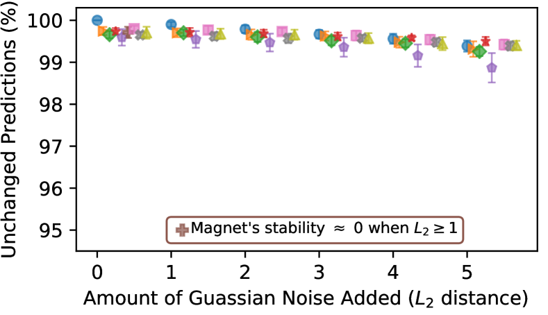
(a) Prediction Stability (MNIST)

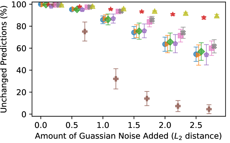
(b) Prediction Stability (Fashion-MNIST)

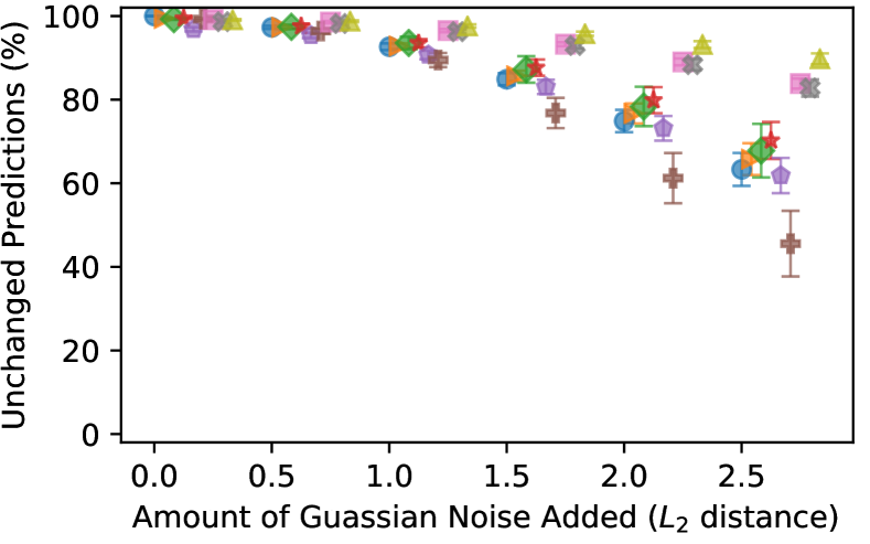
(c) Prediction Stability (CIFAR-10)

Figure 1. Evaluating model stability with Gaussian Noise

(d) Prediction Stability (MNIST)

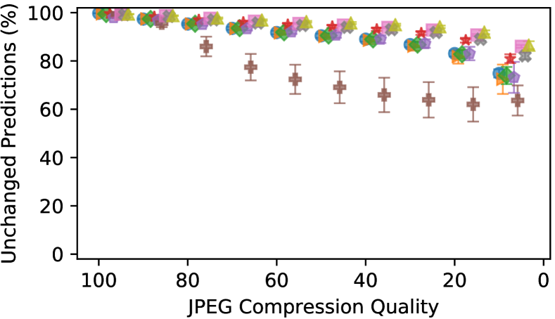
(e) Prediction Stability (Fashion-MNIST)

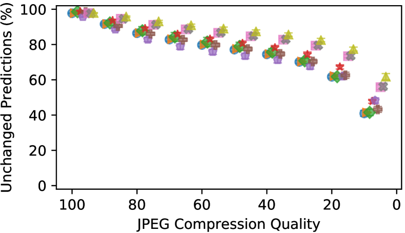
(f) Prediction Stability (CIFAR-10)

Figure 2. Evaluating model stability with JPEG compression

5.3. Model Stability

Given a benign image and its variants with added noise, a more robust model should intuitively be able to tolerate a higher level of noise without changing its prediction results. We refer to this property as model stability. Here we evaluate whether models from a defense mechanism can correct label instances that are perturbed. This serves several purposes. First, in (Gilmer et al., 2019), it is suggested that vulnerability to adversarial examples and low performance on randomly corrupted images, such as images with additive Gaussian noise, are two manifestations of the same underlying phenomenon. Hence it is suggested that adversary defenses should consider robustness under such perturbations, as robustness under such perturbations are also indications of resistance against adversary attacks. Second, evaluating stability is identified in (Carlini et al., 2019; Athalye et al., 2018a) as a way to check whether a defense relies on obfuscated gradients to achieve its defense. For such a defense, random perturbation may discover adversarial examples when optimized search based on gradients fail. Third, some defense mechanisms (such as Magnet) rely on detecting whether an instance belongs to the same distribution as the training set, and consider an instance to be an adversarial example if it does. However, when an input instance goes through some transformation that has little impact on human visual detection (such as JPEG compression), it will be considered as an adversarial example by the defense. This will impact accuracy of deployed systems, as the encountered instances may not always follow the training distribution.

5.3.1. Stability with Added Gaussian Noise

We measure how many predictions would change if a certain amount of Gaussian noise is introduced to a set of benign images. For a given dataset and a model, we use the first $1,000$ images from the test dataset. We first make a prediction on those selected images and store the results as reference predictions. Then, for each selected image and chosen $L_{2}$ distance, we sample Gaussian noise, scale it to the desired $L_{2}$ value, and add the noise to the image. Pixel values are clipped if necessary, to make sure the new noisy variant is a valid image. We repeat this process 20 times (noise sampled independently per iteration).

Fig. 2 shows the effect of Gaussian noise on prediction stability for each training method (averaged over the 16 models trained in Sec. 5.1). Model stability inevitably drops for each scheme as the amount of Gaussian noise as measured by $L_{2}$ increases. However, different schemes behave differently when $L_{2}$ increases.

For MNIST, most schemes have stability above 99%, even when $L_{2}$ is as large as 5. However, Magnet has stability approaching 0 when the $L_{2}$ distance is greater than 1, because majority of those instances are rejected by Magnet.

For Fashion-MNIST, we see more interesting differences among the schemes. The two approaches that have highest stability are the two with adversarial training. When $L_{2}=2.5$, RS-1-ADV has stability 87.4%, and ADV has stability 86%. Other schemes have stability around 60%; among them, RS-1 and RSD-1 have slightly higher stability than others.

For CIFAR-10, we see that RS-1-ADV, RSD-1, and RS-1 have the highest stability as the amount of noise increases. When $L_{2}=2.5$, they have stability 87.9%, 81.7%, 83%, respectively. The other schemes have stability 70% or lower.

Furthermore, on all datasets, RS-1-ADV, RSD-1, and RS-1 give consistent results. Recall that we trained 16 models for each scheme, Fig. 2 also plots the standard deviation of the stability result of the 16 models. RS-1-ADV, RSD-1, and RS-1 have very low standard deviation, which in turn also suggest more consistent behavior when facing perturbed images.

5.3.2. Stability with JPEG compression

Given a set of benign images, we measure how many predictions would change if JPEG compression is applied to images. For a given test dataset and a model, we compare the prediction on the benign test dataset (reference predictions) with the prediction on JPEG compressed test dataset with a fixed chosen JPEG compression quality (JCQ). For the sake of time efficiency, for this particular set of experiments, we reduced the number of iterations used by RC to one-tenth of its original algorithm.

Fig. 2 shows the effect of JPEG compression on prediction stability for each training method (averaged over the 16 models trained). Model stability decreases for each scheme as the JCQ (ranges $10-100$) decreases.

For MNIST, most schemes achieve stability over 99, even if the JCQ is 10. Magnet is the outlier, which has a stability of around 50 when the JCQ is 70, and has a stability of less than 20 when the JCQ is less than or equal to 40, because of the high rejection rate of MagNet. We believe that both of these results are related to the fact that MNIST images have black backgrounds that span most of the image. Noises introduced by JPEG compression result mostly in perturbations in the background that are ignored by most NN models. Since Magnet uses autoencoders to detect deviations from the input distributions, these noises trigger detection. Since Magnet aims at detecting perturbed images, this should not be considered as a weakness of Magnet.

For Fashion-MNIST, we see that RS-1-ADV, RSD-1, and RS-1 outperform other schemes on the stability as the JCQ decreases. When JCQ $=10$, they have stability 85.2%, 80.9%, 84.4%, respectively. The other schemes have stability 80% or lower; The closest to the RS-class among other schemes is ADV.

For CIFAR-10, we see that RS-1-ADV, RSD-1, and RS-1 have the highest stability as the JCQ decreases. When JCQ $=10$, they have stability 60.9%, 55.6%, 55.4%, respectively. The other schemes have stability 50% or lower; the highest among the other schemes is RC.

MNIST

Fashion-MNIST

CIFAR-10

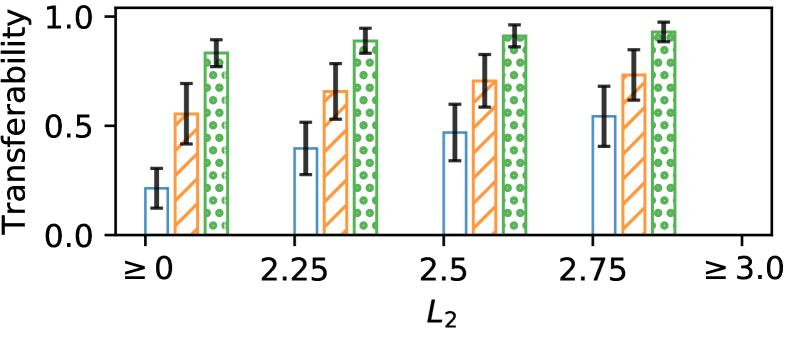
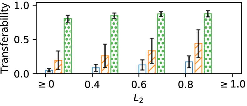
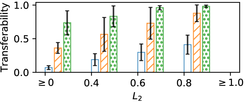
Figure 3. Transferability of adversarial examples found by the 3 attack strategies

5.4. Evaluating Attack Strategies

Here we empirically show that our proposed attack strategy, as presented in Sec. 3.2, can indeed generate adversarial examples that are more transferable. In attacks like the C&W attack, a higher confidence value will typically lead to more transferable examples, but the amount of perturbation would usually increase as well, sometimes making the example noticeably different under human perception.

Intuitively, a better attack strategy should give more transferable adversarial examples using less amount of distortion. Hence we use Distortion vs Transferability to compare $3$ possible attack strategies. Similar to previous experiments, we measure the amount of distortion using $L_{2}$ distance. In Fig. 3 we present the effectiveness of each attack strategy, averaged across the 9 schemes.

The first strategy we evaluated is a standard C&W attack which generates adversarial examples using only one surrogate model, dubbed ‘Single’. Recall that for each training/defense method, we have $16$ models that are surrogates of each other (Sec. 5.1). For each surrogate model, we randomly select half of the original dataset as the training dataset, since the adversary may not have full knowledge of the training dataset under the transfer attack setting. For the Single strategy, we apply the C&W attack on $4$ of the models independently to generate a pool of adversarial examples. The transferability of those examples are then measured and averaged on the remaining $12$ target models. Regardless of the training methods and defense mechanisms in place, adversarial examples generated using the Single strategy often have limited transferability, especially when the allowed amount of distortion ($L_{2}$ distance) is small.

The second attack strategy that we evaluate is to generate adversarial examples using multiple surrogate models. For this, we use $8$ of the $16$ surrogate models for generating attack examples. The C&W attack can be adapted to handle this case with a slightly different loss function. In our experiments, we use the sum of the loss functions of the $8$ surrogate models as the new loss function. We also use slightly lower confidence values than in Sec. 5.1.1 ($\{0,10,20,30\}$ for Fashion-MNIST, $\{0,20,40,60\}$ CIFAR-10). The transferability of the generated adversarial examples are then measured and averaged on the remaining $8$ models as the target. We refer to this as ‘Multi 8’. As shown in Fig. 3, given the same limit on the amount of distortion ($L_{2}$ distance), a significantly higher percentage of examples generated using the Multi 8 strategy are transferable than those found using the Single strategy.

Additionally, we evaluate a third attack strategy that is based on Multi 8. As discussed in Sec. 3.2, given enough surrogate models, one can further use some of them for validating adversarial examples. For those adversarial examples generated by the Multi 8 strategy, we keep them only if they can be transferred to at least $5$ of the $7$ validation models, hence we refer to this strategy Multi 8 & Passing 5/7 Validation. The remaining model is used as the attack target, and we measure the transferability of examples that passed the 5/7 Validation. For this attack strategy, the measurements shown in Fig. 3 is the average of $8$ rotations between target model and validation models. Comparing to Multi 8 and Single, adversarial examples that passed the 5/7 Validation are significantly more likely to transfer to the target model, even when the amount of perturbation is small.

This shows that simple strategies like Single are indeed not realizing the full potential of a resourceful attacker, and our proposed attack strategy of using multiple models for the generation and validation of adversarial examples is indeed superior. In the reset of this section, we will be using the most effective attack strategy of Multi 8 & Passing 5/7 Validation.

5.5. Translucent-box Evaluation

Here we evaluate the effectiveness of different schemes based on the transferability of adversarial examples generated using the Multi 8 & Passing 5/7 Validation attack strategy.

The results of our translucent-box evaluation are shown in Fig. 4(c). Adversarial examples are grouped into buckets based on their $L_{2}$ distance. For each bucket, we use grayscale to indicate the average validation passing rate for each scheme. Passing rate from 0% to 100% are mapped to pixel value from 0 to 255 in a linear scale. There are four rows, each correspond to adversarial examples with a certain $L_{2}$ range. Each column illustrates to what extent a target defense scheme resist adversarial examples generated from attacking different methods.

Examining the columns for Standard and Dropout, we can see that Standard and Dropout are in general most vulnerable. Distillation and RC are almost equally vulnerable. Magnet can often resist adversarial examples generated by targeting other defenses, but are vulnerable to ones generated specifically targeting it.

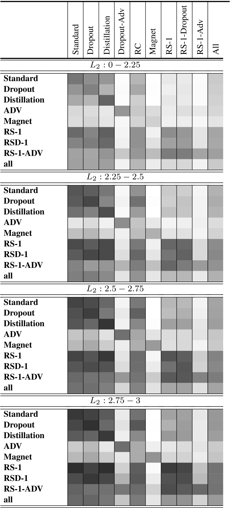
(a) MNIST

(b) Fashion-MNIST

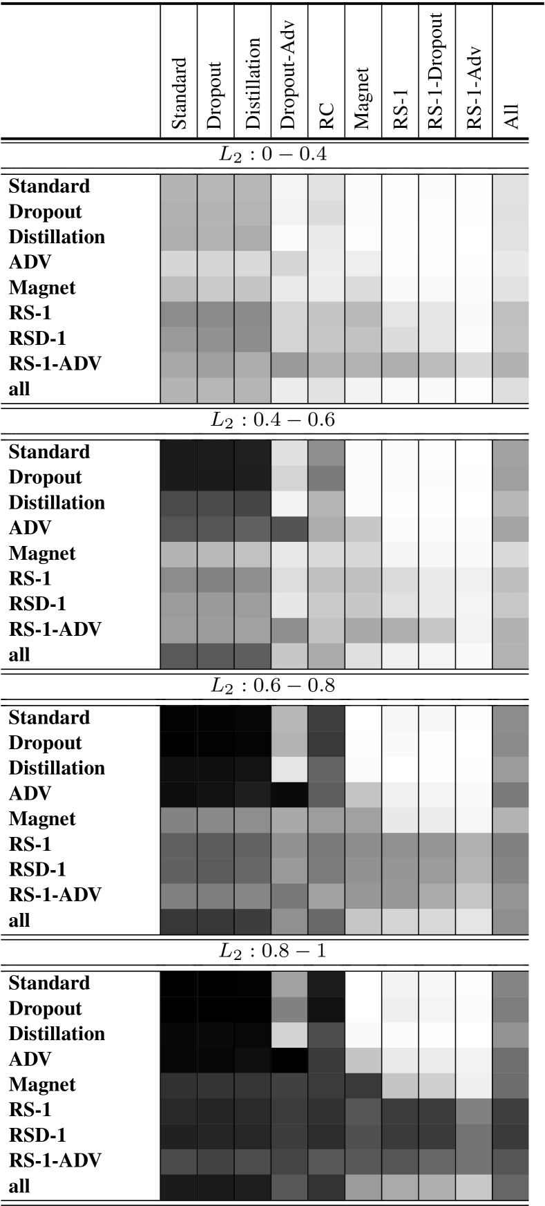
(c) CIFAR-10

Figure 4. Average passing rate of 5/7 validation

This heat map shows the resilience of each scheme against the adversarial examples generated from all schemes, under a fixed allowance of $L_{2}$. Each column illustrates to what extent a target defense scheme resists adversarial examples generated from attacking different methods.

Overall, across the three datasets, RS-1-Adv performs the best, and is significantly better than Dropout-Adv. This suggests that Random Spiking offers additional protection against adversarial examples. RS-1 and RS-1-Dropout also perform consistently well across the three datasets. RC performs noticeably well on MNIST and Fashion-MNIST, likely because the images were all in 8-bit grayscale, and its advantages diminish on CIFAR-10 which contains images of 24-bit color.

6. Related Work

Other attack algorithms. There are other attack algorithms such as JSMA (Papernot et al., 2016a), FGS (Goodfellow et al., 2015), PGD(Madry et al., 2018), and DeepFool (Moosavi-Dezfooli et al., 2016). The general consensus seems to be that the C&W attack is the current state-of-the-art (Carlini and Wagner, 2017b, a; Chen et al., 2018). Though our evaluation results are based on the C&W attack, our evaluation framework is not tied to a particular attack and can use other algorithms.

Other defense mechanisms. Some other defense mechanisms have been proposed (Papernot et al., 2016b; Meng and Chen, 2017; Cao and Gong, 2017; Xu et al., 2018; Xie et al., 2018, 2019) in the literature. For example, Xu et al.. proposed to use feature squeezing techniques such as color bit depths reduction and pixel spatial smoothing to detect adversarial examples (Xu et al., 2018). Xie et al.. proposed to use Feature Denoising (Xie et al., 2019) to improve the robustness of the Neural Network Model. Due to limit in time and space, we selected representative methods from each broad class (e.g., MagNet for the detection approach). We leave comparison with other mechanisms as future work.

Beyond images. Other research efforts have explored possible attacks against neural network models specialized for other purposes, for example, speech to text (Carlini and Wagner, 2018). We focus on images, although the evaluation methodology and the idea of random spiking should be applicable to these other domains.

Alternative similarity metrics. Some researchers have argued that $L_{p}$ norms insufficiently capture human perception, and have proposed alternative similarity metrics like SSIM (Sharif et al., 2018). It is however, not immediately clear how to adapt such metrics in the C&W attack. We leave further investigations on the impacts of alternative similarity metrics on adversarial examples for future work.

7. Conclusion

In this paper, we present a careful analysis of possible adversarial models for studying the phenomenon of adversarial examples. We propose an evaluation methodology that can better illustrate the strengths and limitations of different mechanisms. As part of the method, we introduce a more powerful and meaningful adversary strategy. We also introduce Random Spiking, a randomized technique that generalizes dropout. We have conducted extensive evaluation of Random Spiking and several other defense mechanisms, and demonstrate that Random Spiking, especially when combined with adversarial training, offers better protection against adversarial examples when compared with other existing defenses.

Appendix A Appendix

A.1. More Information on Training

Model architecture and training parameters are in Tables 6 and  7. For MNIST, we use the same as in MagNet (Meng and Chen, 2017; Carlini and Wagner, 2017b)). For Fashion-MNIST and CIFAR-10, they are identical to the WRN (Zagoruyko and Komodakis, 2016). Test errors of the nine schemes are in Table 2. For each scheme and dataset, we train 16 models and report the mean and standard deviation. Additional information is provided below.

Table 6. Mode Architectures. We use WRN-28-10 for Fashion-MNIST and CIFAR-10 ($k=10,N=4$).

MNIST			Fashion-MNIST		CIFAR-10
		Group	Output Size	Kernel, Feature	Output Size	Kernel, Feature
Conv.ReLU	$3\times 3\times 32$	Conv1	$28\times 28$	$[3\times 3,16]$	$32\times 32$	$[3\times 3,16]$
Conv.ReLU	$3\times 3\times 32$	Conv2	$28\times 28$	$\begin{bmatrix}3\times 3,16\times k\\ 3\times 3,16\times k\end{bmatrix}\times N$	$32\times 32$	$\begin{bmatrix}3\times 3,16\times k\\ 3\times 3,16\times k\end{bmatrix}\times N$
Max Pooling	$2\times 2$
Conv.ReLU	$3\times 3\times 64$
Conv.ReLU	$3\times 3\times 64$	Conv3	$14\times 14$	$\begin{bmatrix}3\times 3,32\times k\\ 3\times 3,32\times k\end{bmatrix}\times N$	$16\times 16$	$\begin{bmatrix}3\times 3,32\times k\\ 3\times 3,32\times k\end{bmatrix}\times N$
Max Pooling	$2\times 2$
Dense.ReLU	$200$
Dense.ReLU	$200$	Conv4	$7\times 7$	$\begin{bmatrix}3\times 3,64\times k\\ 3\times 3,64\times k\end{bmatrix}\times N$	$8\times 8$	$\begin{bmatrix}3\times 3,64\times k\\ 3\times 3,64\times k\end{bmatrix}\times N$
Softmax	$10$	Softmax	$10$		$10$

Table 7. Training Parameters.

Parameters	MNIST	Fashion-MNIST & CIFAR-10
Optimization Method	SGD	SGD
Learning Rate	0.01	0.1 initial, multiply by 0.2 at 60, 120 and 160 epochs
Momentum	0.9	0.9
Batch Size	128	128
Epochs	50	200
Dropout (Optional)	0.5	0.1
Data Augmentation	-	Fashion-MNIST: Shifting + Horizontal Flip CIFAR-10: Shifting + Rotation + Horizontal Flip + Zooming + Shear

Magnet. We use the trained Dropout model as the prediction model, and train the Magnet defensive models (reformers and detectors) (Meng and Chen, 2017) based on the publicly released Magnet implementation. Identical to the settings presented in the original Magnet paper (Meng and Chen, 2017), for MNIST, we use Reformer I, Detector I/$L_{2}$ and Detector II/$L_{1}$, with detection threshold set to $0.001$. Since Fashion-MNIST was not studied in (Meng and Chen, 2017), we use the same model architecture as CIFAR-10 presented in the original Magnet paper (Meng and Chen, 2017). For Fashion-MNIST and CIFAR-10, we use Reformer II, Detector II/$L_{1}$, Detector II/$T10$ and Detector II/$T40$, and with a detection threshold (rate of false positive) of $0.004$, which results in test error rates comparable to those of the other schemes.

Random Spiking with standard model (RS-1). A Random Spiking (RS) layer is added after the first convolution layer in the standard architecture. We choose $p=0.8$, so that $20\%$ of all neuron outputs are randomly spiked.

Random Spiking with Dropout (RS-1-Dropout). We add the RS layer to the Dropout scheme. All other parameters are identical to what we used for RS-1. We also use RSD-1 as a shorthand to refer to this scheme.

Distillation. We use the same network architecture and parameters as we did for the training of Dropout models. Identical to the configuration used in (Carlini and Wagner, 2017b), we train with temperature $T=100$ and test with $T=1$ for all three datasets.

Region-based Classification (RC). We use the Dropout models for RC. For each test example, we generate $t$ additional examples, where for each pixel, a noise was randomly chosen from $(-r,r)$ and added to it. Prediction is then made with majority voting on the $t$ input examples. Identical to the original RC paper (Cao and Gong, 2017), we use $t=10,000$ for MNIST and $t=1,000$ for CIFAR-10. We also use $t=1,000$ for Fashion-MNIST. We choose values for $r$ ($r=0.4$ for MNIST, and $r=0.02$ for Fashion-MNIST and CIFAR-10) so that the test errors would be comparable to the other mechanisms.

Adversarial Dropout (Dropout-Adv). To use adversarial training with Dropout, we leverage the trained Dropout model from before as the target model for generating adversarial examples. We generated $12,000$ adversarial examples for each Dropout model by perturbing training instances. To ensure that the adversarial examples indeed should be classified under the original label, we sort the adversarial examples according to their $L_{2}$ distances in ascending order, and add only the first $10,000$ examples into the training dataset. These examples have $L_{2}$ distances lower than the cutoff mentioned earlier. We then apply the Dropout training procedure as described before on the new training dataset.

Adversarial Random Spiking (RS-1-Adv). For this adversarial training method, we use RS-1 as the target model. The training parameters and procedure are largely identical to what were described for Dropout-Adv above.

A.2. Proof of Proposition 1

Proof sketch.

The Monte Carlo sampling used in the RS neural network optimization gives an unbiased estimate of the gradient

$$\sum_{\forall\boldsymbol{b}}\int_{\boldsymbol{\epsilon}}\frac{\partial}{\partial\boldsymbol{W}}L\left(y,\hat{y}(x,\boldsymbol{b},\boldsymbol{\epsilon},\boldsymbol{W})\right)p(\boldsymbol{b})f(\boldsymbol{\epsilon})d\boldsymbol{\epsilon}$$

$$=\frac{\partial}{\partial\boldsymbol{W}}\sum_{\forall\boldsymbol{b}}\int_{\boldsymbol{\epsilon}}L\left(y,\hat{y}(x,\boldsymbol{b},\boldsymbol{\epsilon},\boldsymbol{W})\right)p(\boldsymbol{b})f(\boldsymbol{\epsilon})d\boldsymbol{\epsilon},$$

with the above equality given by the linearity of the expectation and integral operators. That is, the RS neural network optimization is a Robbins-Monro stochastic optimization (Bottou, 2010) that minimizes

$$\boldsymbol{W}^{\prime}=\arg\!\min_{\boldsymbol{W}}\sum_{\forall\boldsymbol{b}}\int_{\boldsymbol{\epsilon}}L(y,\overline{\hat{y}}(x,\boldsymbol{W}))p(\boldsymbol{b})f(\boldsymbol{\epsilon})d\boldsymbol{\epsilon}.$$

$L$ is convex on $\hat{y}$, then by Jensen’s inequality

$$\sum_{\forall\boldsymbol{b}}\int_{\boldsymbol{\epsilon}}L\left(y,\hat{y}(x,\boldsymbol{b},\boldsymbol{\epsilon},\boldsymbol{W})\right)p(\boldsymbol{b})f(\boldsymbol{\epsilon})d\boldsymbol{\epsilon}\geq$$

$$\quad L\left(y,\sum_{\forall\boldsymbol{b}}\int_{\boldsymbol{\epsilon}}\hat{y}(x,\boldsymbol{b},\boldsymbol{\epsilon},\boldsymbol{W})p(\boldsymbol{b})f(\boldsymbol{\epsilon})d\boldsymbol{\epsilon}\right)\equiv L\left(y,\overline{\hat{y}}(x,\boldsymbol{W})\right).$$

Thus, the RS neural network minimizes an upper bound of the loss of the ensemble RS model $\overline{\hat{y}}(x,\boldsymbol{W})$, yielding a proper variational inference procedure (Blei et al., 2017). ∎

References

- (1)
- Athalye et al. (2018a) Anish Athalye, Nicholas Carlini, and David Wagner. 2018a. Obfuscated Gradients Give a False Sense of Security: Circumventing Defenses to Adversarial Examples. In ICML, Vol. 80. PMLR, Stockholmsmässan, Stockholm Sweden, 274–283.
- Athalye et al. (2018b) Anish Athalye, Logan Engstrom, Andrew Ilyas, and Kevin Kwok. 2018b. Synthesizing Robust Adversarial Examples. In ICML, Vol. 80. PMLR, 284–293.
- Blei et al. (2017) David M Blei, Alp Kucukelbir, and Jon D McAuliffe. 2017. Variational inference: A review for statisticians. J. Amer. Statist. Assoc. 112, 518 (2017), 859–877.
- Bottou (2010) Léon Bottou. 2010. Large-scale machine learning with stochastic gradient descent. In Proceedings of COMPSTAT’2010. Springer, 177–186.
- Brendel et al. (2018) Wieland Brendel, Jonas Rauber, and Matthias Bethge. 2018. Decision-Based Adversarial Attacks: Reliable Attacks Against Black-Box Machine Learning Models. In ICLR.
- Cao and Gong (2017) Xiaoyu Cao and Neil Zhenqiang Gong. 2017. Mitigating evasion attacks to deep neural networks via region-based classification. In ACSAC. ACM, 278–287.
- Carlini et al. (2019) Nicholas Carlini, Anish Athalye, Nicolas Papernot, Wieland Brendel, Jonas Rauber, Dimitris Tsipras, Ian J. Goodfellow, Aleksander Madry, and Alexey Kurakin. 2019. On Evaluating Adversarial Robustness. CoRR (2019). arXiv:1902.06705
- Carlini and Wagner (2017a) Nicholas Carlini and David Wagner. 2017a. Adversarial Examples Are Not Easily Detected: Bypassing Ten Detection Methods. In Proceedings of the 10th Workshop on Artificial Intelligence and Security. ACM, 3–14.
- Carlini and Wagner (2017b) Nicholas Carlini and David Wagner. 2017b. Towards evaluating the robustness of neural networks. In 2017 IEEE S&P. IEEE, 39–57.
- Carlini and Wagner (2018) Nicholas Carlini and David Wagner. 2018. Audio Adversarial Examples: Targeted Attacks on Speech-to-Text. Deep Learning and Security Workshop, Article arXiv:1801.01944 (2018), arXiv:1801.01944 pages. arXiv:cs.LG/1801.01944
- Carlini and Wagner (2017c) Nicholas Carlini and David A. Wagner. 2017c. MagNet and “Efficient Defenses Against Adversarial Attacks” are Not Robust to Adversarial Examples. CoRR abs/1711.08478 (2017). arXiv:1711.08478 http://arxiv.org/abs/1711.08478
- Chen and Jordan (2019) Jianbo Chen and Michael I. Jordan. 2019. Boundary Attack++: Query-Efficient Decision-Based Adversarial Attack. (2019). arXiv:1904.02144
- Chen et al. (2018) Pin-Yu Chen, Yash Sharma, Huan Zhang, Jinfeng Yi, and Cho-Jui Hsieh. 2018. EAD: Elastic-Net Attacks to Deep Neural Networks via Adversarial Examples. AAAI Conference on Artificial Intelligence (2018).
- Gal and Ghahramani (2016) Yarin Gal and Zoubin Ghahramani. 2016. Dropout as a Bayesian Approximation: Representing Model Uncertainty in Deep Learning. ICML 48, 1050–1059.
- Gilmer et al. (2019) Justin Gilmer, Nicolas Ford, Nicholas Carlini, and Ekin Cubuk. 2019. Adversarial Examples Are a Natural Consequence of Test Error in Noise. In ICML, Vol. 97. 2280–2289.
- Goodfellow et al. (2015) Ian Goodfellow, Jonathon Shlens, and Christian Szegedy. 2015. Explaining and Harnessing Adversarial Examples. In ICLR.
- Heckman (1977) James J Heckman. 1977. Sample selection bias as a specification error (with an application to the estimation of labor supply functions). (1977).
- Hinton et al. (2014) G. Hinton, O. Vinyals, and J. Dean. 2014. Distilling the Knowledge in a Neural Network. NIPS 2014 Deep Learning and Representation Learning Workshop (2014).
- Kingma and Ba (2015) D. P. Kingma and J. Ba. 2015. Adam: A Method for Stochastic Optimization. In International Conference on Learning Representations.
- Krizhevsky (2009) Alex Krizhevsky. 2009. Learning multiple layers of features from tiny images. Technical Report.
- LeCun et al. (1998) Yann LeCun, Corinna Cortes, and Christopher JC Burges. 1998. The MNIST database of handwritten digits. (1998). http://yann.lecun.com/exdb/mnist/
- Liu et al. (2017) Yanpei Liu, Xinyun Chen, Chang Liu, and Dawn Song. 2017. Delving into Transferable Adversarial Examples and Black-box Attacks. In ICLR.
- Madry et al. (2018) Aleksander Madry, Aleksandar Makelov, Ludwig Schmidt, Dimitris Tsipras, and Adrian Vladu. 2018. Towards deep learning models resistant to adversarial attacks. In ICLR.
- Meng and Chen (2017) Dongyu Meng and Hao Chen. 2017. Magnet: a two-pronged defense against adversarial examples. In CCS. ACM, 135–147.
- Moosavi-Dezfooli et al. (2016) Seyed-Mohsen Moosavi-Dezfooli, Alhussein Fawzi, and Pascal Frossard. 2016. Deepfool: a simple and accurate method to fool deep neural networks. In CVPR. 2574–2582.
- Papernot et al. (2016a) Nicolas Papernot, Patrick McDaniel, Somesh Jha, Matt Fredrikson, Z Berkay Celik, and Ananthram Swami. 2016a. The limitations of deep learning in adversarial settings. In 2016 EuroS&P. IEEE, 372–387.
- Papernot et al. (2016b) Nicolas Papernot, Patrick D. McDaniel, Xi Wu, Somesh Jha, and Ananthram Swami. 2016b. Distillation as a Defense to Adversarial Perturbations Against Deep Neural Networks. In 2016 IEEE S&P. 582–597.
- Sharif et al. (2018) Mahmood Sharif, Lujo Bauer, and Michael K. Reiter. 2018. On the Suitability of L-norms for Creating and Preventing Adversarial Examples. IEEE CVPRW.
- Shimodaira (2000) Hidetoshi Shimodaira. 2000. Improving predictive inference under covariate shift by weighting the log-likelihood function. Journal of statistical planning and inference 90, 2 (2000), 227–244.
- Srivastava et al. (2014) Nitish Srivastava, Geoffrey Hinton, Alex Krizhevsky, Ilya Sutskever, and Ruslan Salakhutdinov. 2014. Dropout: a simple way to prevent neural networks from overfitting. The Journal of Machine Learning Research 15, 1 (2014), 1929–1958.
- Sugiyama et al. (2017) Masashi Sugiyama, Neil D Lawrence, Anton Schwaighofer, et al. 2017. Dataset shift in machine learning. The MIT Press.
- Sugiyama et al. (2008) Masashi Sugiyama, Shinichi Nakajima, Hisashi Kashima, Paul V Buenau, and Motoaki Kawanabe. 2008. Direct importance estimation with model selection and its application to covariate shift adaptation. In Advances in neural information processing systems. 1433–1440.
- Szegedy et al. (2014) Christian Szegedy, Wojciech Zaremba, Ilya Sutskever, Joan Bruna, Dumitru Erhan, Ian Goodfellow, and Rob Fergus. 2014. Intriguing properties of neural networks. In International Conference on Learning Representations.
- Tsipras et al. (2019) Dimitris Tsipras, Shibani Santurkar, Logan Engstrom, Alexander Turner, and Aleksander Madry. 2019. Robustness may be at odds with accuracy. In ICLR.
- Vincent et al. (2008) Pascal Vincent, Hugo Larochelle, Yoshua Bengio, and Pierre-Antoine Manzagol. 2008. Extracting and Composing Robust Features with Denoising Autoencoders. In ICML. ACM, 1096–1103.
- Vincent et al. (2010) Pascal Vincent, Hugo Larochelle, Isabelle Lajoie, Yoshua Bengio, and Pierre-Antoine Manzagol. 2010. Stacked Denoising Autoencoders: Learning Useful Representations in a Deep Network with a Local Denoising Criterion. In ICML, Vol. 11. 3371–3408.
- Wang et al. (2018) Siyue Wang, Xiao Wang, Pu Zhao, Wujie Wen, David Kaeli, Peter Chin, and Xue Lin. 2018. Defensive Dropout for Hardening Deep Neural Networks Under Adversarial Attacks. In ICCAD. ACM, Article 71, 8 pages.
- Xiao et al. (2017) Han Xiao, Kashif Rasul, and Roland Vollgraf. 2017. Fashion-MNIST: a Novel Image Dataset for Benchmarking Machine Learning Algorithms. CoRR abs/1708.07747 (2017). arXiv:1708.07747
- Xie et al. (2018) Cihang Xie, Jianyu Wang, Zhishuai Zhang, Zhou Ren, and Alan L. Yuille. 2018. Mitigating adversarial effects through randomization. ICLR (2018).
- Xie et al. (2019) Cihang Xie, Yuxin Wu, Laurens van der Maaten, Alan L. Yuille, and Kaiming He. 2019. Feature Denoising for Improving Adversarial Robustness. In CVPR.
- Xu et al. (2018) Weilin Xu, David Evans, and Yanjun Qi. 2018. Feature Squeezing: Detecting Adversarial Examples in Deep Neural Networks. NDSS.
- Zagoruyko and Komodakis (2016) Sergey Zagoruyko and Nikos Komodakis. 2016. Wide Residual Networks. In BMVC.
- Zhang et al. (2019) Hongyang Zhang, Yaodong Yu, Jiantao Jiao, Eric P. Xing, Laurent El Ghaoui, and Michael I. Jordan. 2019. Theoretically Principled Trade-off between Robustness and Accuracy. In ICML. 7472–7482.