Moment Matching for Multi-Source Domain Adaptation

Abstract

Conventional unsupervised domain adaptation (UDA) assumes that training data are sampled from a single domain. This neglects the more practical scenario where training data are collected from multiple sources, requiring multi-source domain adaptation. We make three major contributions towards addressing this problem. First, we collect and annotate by far the largest UDA dataset, called DomainNet, which contains six domains and about 0.6 million images distributed among 345 categories, addressing the gap in data availability for multi-source UDA research. Second, we propose a new deep learning approach, Moment Matching for Multi-Source Domain Adaptation (M³SDA), which aims to transfer knowledge learned from multiple labeled source domains to an unlabeled target domain by dynamically aligning moments of their feature distributions. Third, we provide new theoretical insights specifically for moment matching approaches in both single and multiple source domain adaptation. Extensive experiments are conducted to demonstrate the power of our new dataset in benchmarking state-of-the-art multi-source domain adaptation methods, as well as the advantage of our proposed model. Dataset and Code are available at http://ai.bu.edu/M3SDA/

1 Introduction

Generalizing models learned on one visual domain to novel domains has been a major obstacle in the quest for universal object recognition. The performance of the learned models degrades significantly when testing on novel domains due to the presence of domain shift [36].

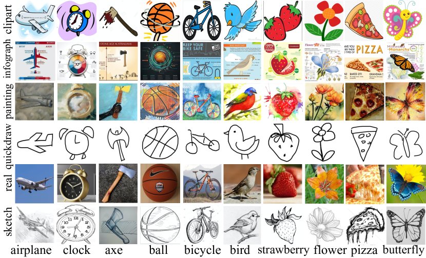
Figure 1: We address Multi-Source Domain Adaptation where source images come from multiple domains. We collect a large scale dataset, DomainNet, with six domains, 345 categories, and $\sim$0.6 million images and propose a model (M³SDA) to transfer knowledge from multiple source domains to an unlabeled target domain.

Recently, transfer learning and domain adaptation methods have been proposed to mitigate the domain gap. For example, several UDA methods [27, 41, 25] incorporate Maximum Mean Discrepancy loss into a neural network to diminish the domain discrepancy; other models introduce different learning schema to align the source and target domains, including aligning second order correlation [39, 32], moment matching [47], adversarial domain confusion [40, 8, 38] and GAN-based alignment [50, 15, 23]. However, most of current UDA methods assume that source samples are collected from a single domain. This assumption neglects the more practical scenarios where labeled images are typically collected from multiple domains. For example, the training images can be taken under different weather or lighting conditions, share different visual cues, and even have different modalities (as shown in Figure 1).

In this paper, we consider multi-source domain adaptation (MSDA), a more difficult but practical problem of knowledge transfer from multiple distinct domains to one unlabeled target domain. The main challenges in the research of MSDA are that: (1) the source data has multiple domains, which hampers the effectiveness of mainstream single UDA method; (2) source domains also possess domain shift with each other; (3) the lack of large-scale multi-domain dataset hinders the development of MSDA models.

In the context of MSDA, some theoretical analysis [1, 28, 4, 49, 14] has been proposed for multi-source domain adaptation (MSDA). Ben-David et al [1] pioneer this direction by introducing an $\mathcal{H}\Delta\mathcal{H}$-divergence between the weighted combination of source domains and target domain. More applied works [6, 45] use an adversarial discriminator to align the multi-source domains with the target domain. However, these works focus only on aligning the source domains with the target, neglecting the domain shift between the source domains. Moreover, $\mathcal{H}\Delta\mathcal{H}$-divergence based analysis does not directly correspond to moment matching approaches.

Dataset	Year	Images	Classes	Domains	Description
Digit-Five	-	$\sim$100,000	10	5	digit
Office [37]	2010	4,110	31	3	office
Office-Caltech [11]	2012	2,533	10	4	office
CAD-Pascal [33]	2015	12,000	20	6	animal,vehicle
Office-Home [43]	2017	15,500	65	4	office, home
PACS [21]	2017	9,991	7	4	animal, stuff
Open MIC [17]	2018	16,156	-	-	museum
Syn2Real [35]	2018	280,157	12	3	animal,vehicle
DomainNet (Ours)	-	569,010	345	6	see Appendix

Table 1: A collection of most notable datasets to evaluate domain adaptation methods. Specifically, “Digit-Five” dataset indicates five most popular digit datasets (MNIST [19], MNIST-M [8], Synthetic Digits [8], SVHN, and USPS) which are widely used to evaluate domain adaptation models. Our dataset is challenging as it contains more images, categories, and domains than other datasets. (see Table 10, Table 11, and Table 12 in Appendix for detailed categories.)

In terms of data, research has been hampered due to the lack of large-scale domain adaptation datasets, as state-of-the-art datasets contain only a few images or have a limited number of classes. Many domain adaptation models exhibit saturation when evaluated on these datasets. For example, many methods achieve $\sim$90 accuracy on the popular Office [37] dataset; Self-Ensembling [7] reports $\sim$99% accuracy on the “Digit-Five” dataset and $\sim$92% accuracy on Syn2Real [35] dataset.

In this paper, we first collect and label a new multi-domain dataset called DomainNet, aiming to overcome benchmark saturation. Our dataset consists of six distinct domains, 345 categories and $\sim$0.6 million images. A comparison of DomainNet and several existing datasets is shown in Table 1, and example images are illustrated in Figure 1. We evaluate several state-of-the-art single domain adaptation methods on our dataset, leading to surprising findings (see Section 5). We also extensively evaluate our model on existing datasets and on DomainNet and show that it outperforms the existing single- and multi-source approaches.

Secondly, we propose a novel approach called M³SDA to tackle MSDA task by aligning the source domains with the target domain, and aligning the source domains with each other simultaneously. We dispose multiple complex adversarial training procedures presented in [45], but directly align the moments of their deep feature distributions, leading to a more robust and effective MSDA model. To our best knowledge, we are the first to empirically demonstrate that aligning the source domains is beneficial for MSDA tasks.

Finally, we extend existing theoretical analysis [1, 14, 49] to the case of moment-based divergence between source and target domains, which provides new theoretical insight specifically for moment matching approaches in domain adaptation, including our approach and many others.

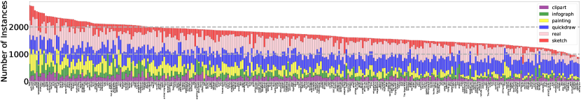
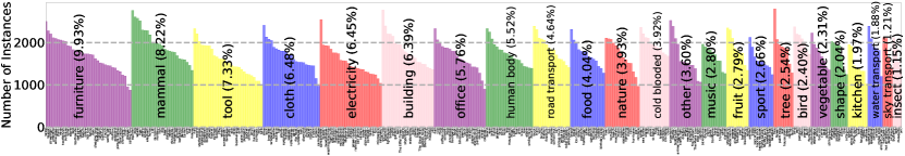
Figure 2: Statistics for our DomainNet dataset. The two plots show object classes sorted by the total number of instances. The top figure shows the percentages each domain takes in the dataset. The bottom figure shows the number of instances grouped by 24 different divisions. Detailed numbers are shown in Table 10, Table 11 and Table 12 in Appendix. (Zoom in to see the exact class names!)

2 Related Work

Domain Adaptation Datasets Several notable datasets that can be utilized to evaluate domain adaptation approaches are summarized in Table 1. The Office dataset [37] is a popular benchmark for office environment objects. It contains 31 categories captured in three domains: office environment images taken with a high quality camera (DSLR), office environment images taken with a low quality camera (Webcam), and images from an online merchandising website (Amazon). The office dataset and its extension, Office-Caltech10 [11], have been used in numerous domain adaptation papers [25, 40, 27, 39, 45], and the adaptation performance has reached $\sim$90% accuracy. More recent benchmarks [43, 17, 34] are proposed to evaluate the effectiveness of domain adaptation models. However, these datasets are small-scale and limited by their specific environments, such as office, home, and museum. Our dataset contains about 600k images, distributed in 345 categories and 6 distinct domains. We capture various object divisions, ranging from furniture, cloth, electronic to mammal, building, etc.

Single-source UDA Over the past decades, various single-source UDA methods have been proposed. These methods can be taxonomically divided into three categories. The first category is the discrepancy-based DA approach, which utilizes different metric learning schemas to diminish the domain shift between source and target domains. Inspired by the kernel two-sample test [12], Maximum Mean Discrepancy (MMD) is applied to reduce distribution shift in various methods [27, 41, 9, 44]. Other commonly used methods include correlation alignment [39, 32], Kullback-Leibler (KL) divergence [51], and $\mathcal{H}$ divergence [1]. The second category is the adversarial-based approach [24, 40]. A domain discriminator is leveraged to encourage the domain confusion by an adversarial objective. Among these approaches, generative adversarial networks are widely used to learn domain-invariant features as well to generate fake source or target data. Other frameworks utilize only adversarial loss to bridge two domains. The third category is reconstruction-based, which assumes the data reconstruction helps the DA models to learn domain-invariant features. The reconstruction is obtained via an encoder-decoder [3, 10] or a GAN discriminator, such as dual-GAN [46], cycle-GAN [50], disco-GAN [16], and CyCADA [15]. Though these methods make progress on UDA, few of them consider the practical scenario where training data are collected from multiple sources. Our paper proposes a model to tackle multi-source domain adaptation, which is a more general and challenging scenario.

Multi-Source Domain Adaptation Compared with single source UDA, multi-source domain adaptation assumes that training data from multiple sources are available. Originated from the early theoretical analysis [1, 28, 4], MSDA has many practical applications [45, 6]. Ben-David et al [1] introduce an $\mathcal{H}\Delta\mathcal{H}$-divergence between the weighted combination of source domains and target domain. Crammer et al [4] establish a general bound on the expected loss of the model by minimizing the empirical loss on the nearest k sources. Mansour et al [28] claim that the target hypothesis can be represented by a weighted combination of source hypotheses. In the more applied works, Deep Cocktail Network (DCTN) [45] proposes a k-way domain discriminator and category classifier for digit classification and real-world object recognition. Hoffman et al [14] propose normalized solutions with theoretical guarantees for cross-entropy loss, aiming to provide a solution for the MSDA problem with very practical benefits. Duan et al [6] propose Domain Selection Machine for event recognition in consumer videos by leveraging a large number of loosely labeled web images from different sources. Different from these methods, our model directly matches all the distributions by matching the moments. Moreover, we provide a concrete proof of why matching the moments of multiple distributions works for multi-source domain adaptation.

Moment Matching The moments of distributions have been studied by the machine learning community for a long time. In order to diminish the domain discrepancy between two domains, different moment matching schemes have been proposed. For example, MMD matches the first moments of two distributions. Sun et al [39] propose an approach that matches the second moments. Zhang et al [48] propose to align infinte-dimensional covariance matrices in RKHS. Zellinger et al [47] introduce a moment matching regularizer to match high moments. As the generative adversarial network (GAN) becomes popular, many GAN-based moment matching approaches have been proposed. McGAN  [29] utilizes a GAN to match the mean and covariance of feature distributions. GMMN [22] and MMD GAN [20] are proposed for aligning distribution moments with generative neural networks. Compared to these methods, our work focuses on matching distribution moments for multiple domains and more importantly, we demonstrate that this is crucial for multi-source domain adaptation.

3 The DomainNet dataset

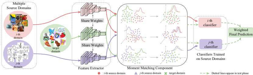
Figure 3: The framework of Moment Matching for Multi-source Domain Adaptation (M³SDA). Our model consists of three components: i) feature extractor, ii) moment matching component, and iii) classifiers. Our model takes multi-source annotated training data as input and transfers the learned knowledge to classify the unlabeled target samples. Without loss of generality, we show the i-th domain and j-th domain as an example. The feature extractor maps the source domains into a common feature space. The moment matching component attempts to match the i-th and j-th domains with the target domain, as well as matching the i-th domain with the j-th domain. The final predictions of target samples are based on the weighted outputs of the i-th and j-th classifiers. (Best viewed in color!)

It is well-known that deep models require massive amounts of training data. Unfortunately, existing datasets for visual domain adaptation are either small-scale or limited in the number of categories. We collect by far the largest domain adaptation dataset to date, DomainNet . The DomainNet contains six domains, with each domain containing 345 categories of common objects, as listed in Table 10, Table 11, and Table 12 (see Appendix). The domains include Clipart (clp, see Appendix, Figure 9): collection of clipart images; Infograph (inf, see Figure 10): infographic images with specific object; Painting (pnt, see Figure 11): artistic depictions of objects in the form of paintings; Quickdraw (qdr, see Figure 12): drawings of the worldwide players of game “Quick Draw!”; Real (rel, see Figure 13): photos and real world images; and Sketch (skt, see Figure 14): sketches of specific objects.

The images from clipart, infograph, painting, real, and sketch domains are collected by searching a category name combined with a domain name (e.g. “aeroplane painting”) in different image search engines. One of the main challenges is that the downloaded data contain a large portion of outliers. To clean the dataset, we hire 20 annotators to manually filter out the outliers. This process took around 2,500 hours (more than 2 weeks) in total. To control the annotation quality, we assign two annotators to each image, and only take the images agreed by both annotators. After the filtering process, we keep 423.5k images from the 1.2 million images crawled from the web. The dataset has an average of around 150 images per category for clipart and infograph domain, around 220 per category for painting and sketch domain, and around 510 for real domain. A statistical overview of the dataset is shown in Figure 2.

The quickdraw domain is downloaded directly from https://quickdraw.withgoogle.com/. The raw data are presented as a series of discrete points with temporal information. We use the B-spline [5] algorithm to connect all the points in each strike to get a complete drawing. We choose 500 images for each category to form the quickdraw domain, which contains 172.5k images in total.

4 Moment Matching for Multi-Source DA

Given ${\mathcal{D}}_{S}=\{{\mathcal{D}}_{1},{\mathcal{D}}_{2},...,{\mathcal{D}}_{N}\}$ the collection of labeled source domains and ${\mathcal{D}}_{T}$ the unlabeled target domain, where all domains are defined by bounded rational measures on input space ${\mathcal{X}}$, the multi-source domain adaptation problem aims to find a hypothesis in the given hypothesis space ${\mathcal{H}}$, which minimizes the testing target error on ${\mathcal{D}}_{T}$.

Definition 1.

Assume ${\mathbf{X}}_{1}$, ${\mathbf{X}}_{2}$ $,...,$ ${\mathbf{X}}_{N}$, ${\mathbf{X}}_{T}$ are collections of i.i.d. samples from ${\mathcal{D}}_{1},{\mathcal{D}}_{2},...,{\mathcal{D}}_{N},{\mathcal{D}}_{T}$ respectively, then the Moment Distance between ${\mathcal{D}}_{S}$ and ${\mathcal{D}}_{T}$ is defined as

$$MD^{2}({\mathcal{D}}_{S},{\mathcal{D}}_{T})=\sum_{k=1}^{2}\Bigg{(}\frac{1}{N}\sum_{i=1}^{N}\|\mathbb{E}({\mathbf{X}}_{i}^{k})-\mathbb{E}({\mathbf{X}}_{T}^{k})\|_{2}$$

$$+\binom{N}{2}^{-1}\sum_{i=1}^{N-1}\sum_{j=i+1}^{N}\|\mathbb{E}({\mathbf{X}}_{i}^{k})-\mathbb{E}({\mathbf{X}}_{j}^{k})\|_{2}\Bigg{)}.$$ (1)

M³SDA We propose a moment-matching model for MSDA based on deep neural networks. As shown in Figure 3, our model comprises of a feature extractor $G$, a moment-matching component, and a set of $N$ classifiers ${\mathcal{C}}=\{C_{1},C_{2},...,C_{N}\}$. The feature extractor $G$ maps ${\mathcal{D}}_{S}$, ${\mathcal{D}}_{T}$ to a common latent feature space. The moment matching component minimizes the moment-related distance defined in Equation 1. The $N$ classifiers are trained on the annotated source domains with cross-entropy loss. The overall objective function is:

$$\min_{G,{\mathcal{C}}}\sum_{i=1}^{N}{\mathcal{L}}_{{\mathcal{D}}_{i}}+\lambda\min_{G}MD^{2}({\mathcal{D}}_{S},{\mathcal{D}}_{T}),$$ (2)

where ${\mathcal{L}}_{{\mathcal{D}}_{i}}$ is the softmax cross entropy loss for the classifier $C_{i}$ on domain ${\mathcal{D}}_{i}$, and $\lambda$ is the trade-off parameter.

M³SDA assumes that $p(y|x)$ will be aligned automatically when aligning $p(x)$, which might not hold in practice. To mitigate this limitation, we further propose M³SDA-$\beta$.

M³SDA-$\beta$ In order to align $p(y|x)$ and $p(x)$ at the same time, we follow the training paradigm proposed by [38]. In particular, we leverage two classifiers per domain to form $N$ pairs of classifiers ${\mathcal{C}}\textprime=\big{\{}(C_{1},C_{1}\textprime),(C_{2},C_{2}\textprime),...,(C_{N},C_{N}\textprime)\big{\}}$. The training procedure includes three steps. i). We train $G$ and ${\mathcal{C}}\textprime$ to classify the multi-source samples correctly. The objective is similar to Equation 2. ii). We then train the classifier pairs for a fixed $G$. The goal is to make the discrepancy of each pair of classifiers as large as possible on the target domain. For example, the outputs of $C_{1}$ and $C_{1}\textprime$ should possess a large discrepancy. Following [38], we define the discrepancy of two classifiers as the L1-distance between the outputs of the two classifiers. The objective is:

$$\min_{{\mathcal{C}}\textprime}\sum_{i=1}^{N}{\mathcal{L}}_{{\mathcal{D}}_{i}}-\sum_{i}^{N}|P_{C_{i}}(D_{T})-P_{C_{i}\textprime}(D_{T})|,$$ (3)

where $P_{C_{i}}(D_{T})$, $P_{C_{i}\textprime}(D_{T})$ denote the outputs of $C_{i}$, $C_{i}\textprime$ respectively on the target domain. iii). Finally, we fix ${\mathcal{C}}\textprime$ and train $G$ to minimize the discrepancy of each classifier pair on the target domain. The objective function is as follows:

$$\min_{G}\sum_{i}^{N}|P_{C_{i}}(D_{T})-P_{C_{i}\textprime}(D_{T})|,$$ (4)

These three training steps are performed periodically until the whole network converges.

Ensemble Schema In the testing phase, testing data from the target domain are forwarded through the feature generator and the $N$ classifiers. We propose two schemas to combine the outputs of the classifiers:

• average the outputs of the classifiers, marked as M³SDA^∗

• Derive a weight vector ${\mathcal{W}}=(w_{1},\ldots,w_{N-1})$ ($\sum_{i=1}^{N-1}w_{i}=1$, assuming $N$-th domain is the target). The final prediction is the weighted average of the outputs.

To this end, how to derive the weight vector becomes a critical problem. The main philosophy of the weight vector is to make it represent the intrinsic closeness between the target domain and source domains. In our setting, the weighted vector is derived by the source-only accuracy between the $i$-th domain and the $N$-th domain, i.e. $w_{i}=acc_{i}/\sum_{j=1}^{N-1}acc_{j}$.

4.1 Theoretical Insight

Following [1], we introduce a rigorous model of multi-source domain adaptation for binary classification. A domain ${\mathcal{D}}=(\mu,f)$ is defined by a probability measure (distribution) $\mu$ on the input space ${\mathcal{X}}$ and a labeling function $f:{\mathcal{X}}\to\{0,1\}$. A hypothesis is a function $h:{\mathcal{X}}\to\{0,1\}$. The probability that $h$ disagrees with the domain labeling function $f$ under the domain distribution $\mu$ is defined as:

$$\epsilon_{{\mathcal{D}}}(h)=\epsilon_{{\mathcal{D}}}(h,f)=\mathbb{E}_{\mu}\big{[}|h({\bm{x}})-f({\bm{x}})|\big{]}.$$ (5)

For a source domain ${\mathcal{D}}_{S}$ and a target domain ${\mathcal{D}}_{T}$, we refer to the source error and the target error of a hypothesis $h$ as $\epsilon_{S}(h)=\epsilon_{{\mathcal{D}}_{S}}(h)$ and $\epsilon_{T}(h)=\epsilon_{{\mathcal{D}}_{T}}(h)$ respectively. When the expectation in Equation 5 is computed with respect to an empirical distribution, we denote the corresponding empirical error by $\hat{\epsilon}_{{\mathcal{D}}}(h)$, such as $\hat{\epsilon}_{S}(h)$ and $\hat{\epsilon}_{T}(h)$. In particular, we examine algorithms that minimize convex combinations of source errors, i.e., given a weight vector ${\bm{\alpha}}=(\alpha_{1},\ldots,\alpha_{N})$ with $\sum_{j=1}^{N}\alpha_{j}=1$, we define the ${\bm{\alpha}}$-weighted source error of a hypothesis $h$ as $\epsilon_{{\bm{\alpha}}}(h)=\sum_{j=1}^{N}\alpha_{j}\epsilon_{j}(h),$ where $\epsilon_{j}(h)$ is the shorthand of $\epsilon_{{\mathcal{D}}_{j}}(h)$. The empirical ${\bm{\alpha}}$-weighted source error can be defined analogously and denoted by $\hat{\epsilon}_{{\bm{\alpha}}}(h)$.

Previous theoretical bounds [1, 14, 49] on the target error are based on the $\mathcal{H}\Delta\mathcal{H}$-divergence between the source and target domains. While providing theoretical insights for general multi-source domain adaptation, these $\mathcal{H}\Delta\mathcal{H}$-divergence based bounds do not directly motivate moment-based approaches. In order to provide a specific insight for moment-based approaches, we introduce the $k$-th order cross-moment divergence between domains, denoted by $d_{CM^{k}}(\cdot,\cdot)$, and extend the analysis in [1] to derive the following moment-based bound for multi-source domain adaptation. See Appendix for the definition of the cross-moment divergence and the proof of the theorem.

Standards	Models	mt,up,sv,sy $\rightarrow$ mm	mm,up,sv,sy $\rightarrow$ mt	mm,mt,sv,sy $\rightarrow$ up	mm,mt,up,sy $\rightarrow$ sv	mm,mt,up,sv $\rightarrow$ sy	Avg
Source Combine	Source Only	63.70$\pm$0.83	92.30$\pm$0.91	90.71$\pm$0.54	71.51$\pm$0.75	83.44$\pm$0.79	80.33$\pm$0.76
	DAN [25]	67.87$\pm$0.75	97.50$\pm$ 0.62	93.49$\pm$0.85	67.80$\pm$0.84	86.93$\pm$0.93	82.72$\pm$ 0.79
	DANN [8]	70.81$\pm$0.94	97.90$\pm$0.83	93.47$\pm$0.79	68.50$\pm$0.85	87.37$\pm$0.68	83.61$\pm$0.82
Multi- Source	Source Only	63.37$\pm$0.74	90.50$\pm$0.83	88.71$\pm$0.89	63.54$\pm$0.93	82.44$\pm$0.65	77.71$\pm$0.81
	DAN [25]	63.78$\pm$0.71	96.31$\pm$0.54	94.24$\pm$0.87	62.45$\pm$0.72	85.43$\pm$0.77	80.44$\pm$0.72
	CORAL [39]	62.53$\pm$0.69	97.21$\pm$0.83	93.45$\pm$0.82	64.40$\pm$0.72	82.77$\pm$0.69	80.07$\pm$0.75
	DANN [8]	71.30$\pm$0.56	97.60$\pm$0.75	92.33$\pm$0.85	63.48$\pm$0.79	85.34$\pm$0.84	82.01$\pm$0.76
	JAN [27]	65.88$\pm$0.68	97.21$\pm$0.73	95.42$\pm$0.77	75.27$\pm$0.71	86.55$\pm$0.64	84.07$\pm$0.71
	ADDA [40]	71.57$\pm$ 0.52	97.89$\pm$0.84	92.83$\pm$0.74	75.48$\pm$0.48	86.45$\pm$0.62	84.84$\pm$0.64
	DCTN [45]	70.53$\pm$1.24	96.23$\pm$0.82	92.81$\pm$0.27	77.61$\pm$0.41	86.77$\pm$0.78	84.79$\pm$0.72
	MEDA [44]	71.31$\pm$0.75	96.47$\pm$0.78	97.01$\pm$0.82	78.45$\pm$0.77	84.62$\pm$0.79	85.60$\pm$ 0.78
	MCD [38]	72.50$\pm$0.67	96.21$\pm$0.81	95.33$\pm$0.74	78.89$\pm$0.78	87.47$\pm$0.65	86.10$\pm$0.73
	M3SDA (ours)	69.76$\pm$0.86	98.58$\pm$0.47	95.23$\pm$0.79	78.56$\pm$0.95	87.56$\pm$0.53	86.13$\pm$0.64
	M3SDA-$\beta$ (ours)	72.82$\pm$1.13	98.43$\pm$0.68	96.14$\pm$0.81	81.32$\pm$0.86	89.58$\pm$0.56	87.65$\pm$ 0.75

Table 2: Digits Classification Results. mt, up, sv, sy, mm are abbreviations for MNIST, USPS, SVHN, Synthetic Digits, MNIST-M, respectively. Our model M³SDA and M³SDA-$\beta$ achieve 86.13% and 87.65% accuracy, outperforming other baselines by a large margin.

Theorem 1.

Let ${\mathcal{H}}$ be a hypothesis space of $VC$ dimension $d.$ Let $m$ be the size of labeled samples from all sources $\{{\mathcal{D}}_{1},{\mathcal{D}}_{2},...,{\mathcal{D}}_{N}\}$, $S_{j}$ be the labeled sample set of size $\beta_{j}m$ ($\sum_{j}\beta_{j}=1$) drawn from $\mu_{j}$ and labeled by the groundtruth labeling function $f_{j}.$ If $\hat{h}\in{\mathcal{H}}$ is the empirical minimizer of $\hat{\epsilon}_{{\bm{\alpha}}}(h)$ for a fixed weight vector ${\bm{\alpha}}$ and $h^{*}_{T}=\min_{h\in{\mathcal{H}}}\epsilon_{T}(h)$ is the target error minimizer, then for any $\delta\in(0,1)$ and any $\epsilon>0$, there exist $N$ integers $\{n^{j}_{\epsilon}\}_{j=1}^{N}$ and $N$ constants $\{a_{n^{j}_{\epsilon}}\}_{j=1}^{N}$, such that with probability at least $1-\delta,$

$$\begin{split}\epsilon_{T}(\hat{h})\leq&\ \epsilon_{T}(h^{*}_{T})+\eta_{{\bm{\alpha}},{\bm{\beta}},m,\delta}+\epsilon\\ &+\sum_{j=1}^{N}\alpha_{j}\bigg{(}2\lambda_{j}+a_{n^{j}_{\epsilon}}\sum_{k=1}^{n^{j}_{\epsilon}}d_{CM^{k}}\big{(}{\mathcal{D}}_{j},{\mathcal{D}}_{T}\big{)}\bigg{)},\end{split}$$ (6)

where $\eta_{{\bm{\alpha}},{\bm{\beta}},m,\delta}=4\sqrt{\Big{(}\sum_{j=1}^{N}\frac{\alpha_{j}^{2}}{\beta_{j}}\Big{)}\Big{(}\frac{2d(\log(\frac{2m}{d})+1)+2\log(\frac{4}{\delta})}{m}\Big{)}}$ and $\lambda_{j}=\min_{h\in{\mathcal{H}}}\{\epsilon_{T}(h)+\epsilon_{j}(h)\}.$

Theorem 1 shows that the upper bound on the target error of the learned hypothesis depends on the pairwise moment divergence $d_{CM^{k}}\big{(}{\mathcal{D}}_{S},{\mathcal{D}}_{T}\big{)}$ between the target domain and each source domain. This provides a direct motivation for moment matching approaches beyond ours. In particular, it motivates our multi-source domain adaptation approach to align the moments between each target-source pair. Moreover, it is obvious that the last term of the bound, $\sum_{k}d_{CM^{k}}\big{(}{\mathcal{D}}_{j},{\mathcal{D}}_{T}\big{)}$, is lower bounded by the pairwise divergences between source domains. To see this, consider the toy example consisting of two sources ${\mathcal{D}}_{1},{\mathcal{D}}_{2}$, and a target ${\mathcal{D}}_{T},$ since $d_{CM^{k}}(\cdot,\cdot)$ is a metric, triangle inequality implies the following lower bound:

$$d_{CM^{k}}\big{(}{\mathcal{D}}_{1},{\mathcal{D}}_{T}\big{)}+d_{CM^{k}}\big{(}{\mathcal{D}}_{2},{\mathcal{D}}_{T}\big{)}\geq d_{CM^{k}}\big{(}{\mathcal{D}}_{1},{\mathcal{D}}_{2}\big{)}.$$

This motivates our algorithm to also align the moments between each pair of source domains. Intuitively, it is not possible to perfectly align the target domain with every source domain, if the source domains are not aligned themselves. Further discussions of Theorem 1 and its relationship with our algorithm are provided in the Appendix.

5 Experiments

We perform an extensive evaluation on the following tasks: digit classification (MNIST, SVHN, USPS, MNIST-M, Sythetic Digits), and image recognition (Office-Caltech10, DomainNet dataset). In total, we conduct 714 experiments. The experiments are run on a GPU-cluster with 24 GPUs and the total running time is more than 21,440 GPU-hours. Due to space limitations, we only report major results; more implementation details are provided in the supplementary material. Throughout the experiments, we set the trade-off parameter $\lambda$ in Equation  2 as 0.5. In terms of the parameter sensitivity, we have observed that the performance variation is not significant if $\lambda$ is between 0.1$\sim$1. All of our experiments are implemented in the PyTorch platform.

AlexNet	clp	inf	pnt	qdr	rel	skt	Avg.	DAN	clp	inf	pnt	qdr	rel	skt	Avg.	JAN	clp	inf	pnt	qdr	rel	skt	Avg.	DANN	clp	inf	pnt	qdr	rel	skt	Avg.
clp	65.5	8.2	21.4	10.5	36.1	10.8	17.4	clp	N/A	9.1	23.4	16.2	37.9	29.7	23.2	clp	N/A	7.8	24.5	14.3	38.1	25.7	22.1	clp	N/A	9.1	23.2	13.7	37.6	28.6	22.4
inf	32.9	27.7	23.8	2.2	26.4	13.7	19.8	inf	17.2	N/A	15.6	4.4	24.8	13.5	15.1	inf	17.6	N/A	18.7	8.7	28.1	15.3	17.7	inf	17.9	N/A	16.4	2.1	27.8	13.3	15.5
pnt	28.1	7.5	57.6	2.6	41.6	20.8	20.1	pnt	29.9	8.9	N/A	7.9	42.1	26.1	23.0	pnt	27.5	8.2	N/A	7.1	43.1	23.9	22.0	pnt	29.1	8.6	N/A	5.1	41.5	24.7	21.8
qdr	13.4	1.2	2.5	68.0	5.5	7.1	5.9	qdr	14.2	1.6	4.4	N/A	8.5	10.1	7.8	qdr	17.8	2.2	7.4	N/A	8.1	10.9	9.3	qdr	16.8	1.8	4.8	N/A	9.3	10.2	8.6
rel	36.9	10.2	33.9	4.9	72.8	23.1	21.8	rel	37.4	11.5	33.3	10.1	N/A	26.4	23.7	rel	33.5	9.1	32.5	7.5	N/A	21.9	20.9	rel	36.5	11.4	33.9	5.9	N/A	24.5	22.4
skt	35.5	7.1	21.9	11.8	30.8	56.3	21.4	skt	39.1	8.8	28.2	13.9	36.2	N/A	25.2	skt	35.3	8.2	27.7	13.3	36.8	N/A	24.3	skt	37.9	8.2	26.3	12.2	35.3	N/A	24.0
Avg.	29.4	6.8	20.7	6.4	28.1	15.1	17.8	Avg.	27.6	8.0	21.0	10.5	29.9	21.2	19.7	Avg.	26.3	7.1	22.2	10.2	30.8	19.5	19.4	Avg.	27.6	7.8	20.9	7.8	30.3	20.3	19.1
RTN	clp	inf	pnt	qdr	rel	skt	Avg.	ADDA	clp	inf	pnt	qdr	rel	skt	Avg.	MCD	clp	inf	pnt	qdr	rel	skt	Avg.	SE	clp	inf	pnt	qdr	rel	skt	Avg.
clp	N/A	8.1	21.1	13.1	36.1	26.5	21.0	clp	N/A	11.2	24.1	3.2	41.9	30.7	22.2	clp	N/A	14.2	26.1	1.6	45.0	33.8	24.1	clp	N/A	9.7	12.2	2.2	33.4	23.1	16.1
inf	15.6	N/A	15.3	3.4	25.1	12.8	14.4	inf	19.1	N/A	16.4	3.2	26.9	14.6	16.0	inf	23.6	N/A	21.2	1.5	36.7	18.0	20.2	inf	10.3	N/A	9.6	1.2	13.1	6.9	8.2
pnt	26.8	8.1	N/A	5.2	40.6	22.6	20.7	pnt	31.2	9.5	N/A	8.4	39.1	25.4	22.7	pnt	34.4	14.8	N/A	1.9	50.5	28.4	26.0	pnt	17.1	9.4	N/A	2.1	28.4	15.9	14.6
qdr	15.1	1.8	4.5	N/A	8.5	8.9	7.8	qdr	15.7	2.6	5.4	N/A	9.9	11.9	9.1	qdr	15.0	3.0	7.0	N/A	11.5	10.2	9.3	qdr	13.6	3.9	11.6	N/A	16.4	11.5	11.4
rel	35.3	10.7	31.7	7.5	N/A	22.9	21.6	rel	39.5	14.5	29.1	12.1	N/A	25.7	24.2	rel	42.6	19.6	42.6	2.2	N/A	29.3	27.2	rel	31.7	12.9	19.9	3.7	N/A	26.3	18.9
skt	34.1	7.4	23.3	12.6	32.1	N/A	21.9	skt	35.3	8.9	25.2	14.9	37.6	N/A	25.4	skt	41.2	13.7	27.6	3.8	34.8	N/A	24.2	skt	18.7	7.8	12.2	7.7	28.9	N/A	15.1
Avg.	25.4	7.2	19.2	8.4	28.4	18.7	17.9	Avg.	28.2	9.3	20.1	8.4	31.1	21.7	19.8	Avg.	31.4	13.1	24.9	2.2	35.7	23.9	21.9	Avg.	18.3	8.7	13.1	3.4	24.1	16.7	14.1

Table 3: Single-source baselines on the DomainNet dataset. Several single-source adaptation baselines are evaluated on the DomainNet dataset, including AlexNet [18], DAN [25], JAN [27], DANN [8], RTN [26], ADDA [40], MCD [38], SE [7]. In each sub-table, the column-wise domains are selected as the source domain and the row-wise domains are selected as the target domain. The green numbers represent the average performance of each column or row. The red numbers denote the average accuracy for all the 30 (source, target) combinations.

Standards	Models	A,C,D $\rightarrow$W	A,C,W $\rightarrow$D	A,D,W $\rightarrow$C	C,D,W $\rightarrow$A	Avg
Source Combine	Source only	99.0	98.3	87.8	86.1	92.8
	DAN [25]	99.3	98.2	89.7	94.8	95.5
Multi-Source	Source only	99.1	98.2	85.4	88.7	92.9
	DAN [25]	99.5	99.1	89.2	91.6	94.8
	DCTN [45]	99.4	99.0	90.2	92.7	95.3
	JAN [27]	99.4	99.4	91.2	91.8	95.5
	MEDA [44]	99.3	99.2	91.4	92.9	95.7
	MCD [38]	99.5	99.1	91.5	92.1	95.6
	M3SDA (ours)	99.4	99.2	91.5	94.1	96.1
	M3SDA-$\beta$ (ours)	99.5	99.2	92.2	94.5	96.4

Table 4: Results on Office-Caltech10 dataset. A,C,W and D represent Amazon, Caltech, Webcam and DSLR, respectively. All the experiments are based on ResNet-101 pre-trained on ImageNet.

5.1 Experiments on Digit Recognition

Five digit datasets are sampled from five different sources, namely MNIST [19], Synthetic Digits [8], MNIST-M [8], SVHN, and USPS. Following DCTN [45], we sample 25000 images from training subset and 9000 from testing subset in MNIST, MINST-M, SVHN, and Synthetic Digits. USPS dataset contains only 9298 images in total, so we take the entire dataset as a domain. In all of our experiments, we take turns to set one domain as the target domain and the rest as the source domains.

We take four state-of-the-art discrepancy-based approaches: Deep Adaptation Network [25] (DAN), Joint Adaptation Network (JAN), Manifold Embedded Distribution Alignment (MEDA), and Correlation Alignment [39] (CORAL), and four adversarial-based approaches: Domain Adversarial Neural Network [8] (DANN), Adversarial Discriminative Domain Adaptation [40] (ADDA), Maximum Classifier Discrepancy (MCD) and Deep Cocktail Network [45] (DCTN) as our baselines. In the source combine setting, all the source domains are combined to a single domain, and the baseline experiments are conducted in a traditional single domain adaptation manner.

The results are shown in Table 2. Our model M³SDA achieves an 86.13% average accuracy, and M³SDA-$\beta$ boosts the performance to 87.65%, outperforming other baselines by a large margin. One interesting observation is that the results on MNIST-M dataset is lower. This phenomenon is probably due to the presence of negative transfer [31]. For a fair comparison, all the experiments are based on the same network architecture. For each experiment, we run the same setting for five times and report the mean and standard deviation. (See Appendix for detailed experiment settings and analyses.)

5.2 Experiments on Office-Caltech10

The Office-Caltech10 [11] dataset is extended from the standard Office31 [37] dataset. It consists of the same 10 object categories from 4 different domains: Amazon, Caltech, DSLR, and Webcam.

The experimental results on Office-Caltech10 dataset are shown in Table 5. Our model M³SDA gets a 96.1% average accuracy on this dataset, and M³SDA-$\beta$ further boosts the performance to 96.4%. All the experiments are based on ResNet-101 pre-trained on ImageNet. As far as we know, our models achieve the best performance among all the results ever reported on this dataset. We have also tried AlexNet, but it did not work as well as ResNet-101.

5.3 Experiments on DomainNet

Single-Source Adaptation To demonstrate the intrinsic difficulty of DomainNet, we evaluate multiple state-of-the-art algorithms for single-source adaptation: Deep Alignment Network (DAN) [25], Joint Adaptation Network (JAN) [27], Domain Adversarial Neural Network (DANN) [8], Residual Transfer Network (RTN) [26], Adversarial Deep Domain Adaptation (ADDA) [40], Maximum Classifier Discrepancy (MCD) [38], and Self-Ensembling (SE) [7]. As the DomainNet dataset contains 6 domains, experiments for 30 different (sources, target) combinations are performed for each baseline. For each domain, we follow a 70%/30% split scheme to participate our dataset into training and testing trunk. The detailed statistics can be viewed in Table 8 (see Appendix). All other experimental settings (neural network, learning rate, stepsize, etc.) are kept the same as in the original papers. Specifically, DAN, JAN, DANN, and RTN are based on AlexNet [18], ADDA and MCD are based on ResNet-101 [13], and SE is based on ResNet-152 [13]. Table 3 shows all the source-only and experimental results. (Source-only results for ResNet-101 and ResNet-152 are in Appendix, Table 7). The results show that our dataset is challenging, especially for the infograph and quickdraw domain. We argue that the difficulty is mainly introduced by the large number of categories in our dataset.

Figure 4: Accuracy vs. Number of categories. This plot shows the painting$\rightarrow$real scenario. More plots with similar trend can be accessed in Figure  5 (see Appendix).

Standards	Models	inf,pnt,qdr, rel,skt$\rightarrow$clp	clp,pnt,qdr, rel,skt$\rightarrow$inf	clp,inf,qdr, rel,skt$\rightarrow$pnt	clp,inf,pnt, rel,skt$\rightarrow$qdr	clp,inf,pnt, qdr,skt $\rightarrow$rel	clp,inf,pnt, qdr,rel $\rightarrow$skt	Avg
Single Best	Source Only	39.6$\pm$0.58	8.2$\pm$0.75	33.9 $\pm$ 0.62	11.8 $\pm$ 0.69	41.6 $\pm$ 0.84	23.1$\pm$0.72	26.4 $\pm$ 0.70
	DAN [25]	39.1$\pm$0.51	11.4$\pm$0.81	33.3$\pm$0.62	16.2$\pm$0.38	42.1$\pm$0.73	29.7$\pm$0.93	28.6$\pm$0.63
	RTN [26]	35.3$\pm$0.73	10.7$\pm$0.61	31.7$\pm$0.82	13.1$\pm$0.68	40.6$\pm$0.55	26.5$\pm$0.78	26.3$\pm$0.70
	JAN [27]	35.3$\pm$0.71	9.1$\pm$0.63	32.5$\pm$0.65	14.3$\pm$0.62	43.1$\pm$0.78	25.7$\pm$0.61	26.7$\pm$0.67
	DANN [8]	37.9$\pm$0.69	11.4$\pm$0.91	33.9$\pm$0.60	13.7$\pm$0.56	41.5$\pm$0.67	28.6$\pm$0.63	27.8$\pm$0.68
	ADDA [40]	39.5$\pm$0.81	14.5$\pm$0.69	29.1$\pm$0.78	14.9$\pm$0.54	41.9$\pm$0.82	30.7$\pm$0.68	28.4$\pm$0.72
	SE [7]	31.7$\pm$0.70	12.9$\pm$0.58	19.9$\pm$0.75	7.7$\pm$0.44	33.4$\pm$0.56	26.3$\pm$0.50	22.0$\pm$0.66
	MCD [38]	42.6$\pm$0.32	19.6$\pm$0.76	42.6$\pm$0.98	3.8$\pm$0.64	50.5$\pm$0.43	33.8$\pm$0.89	32.2$\pm$0.66
Source Combine	Source Only	47.6$\pm$0.52	13.0$\pm$0.41	38.1$\pm$0.45	13.3$\pm$0.39	51.9$\pm$0.85	33.7$\pm$0.54	32.9$\pm$0.54
	DAN [25]	45.4$\pm$0.49	12.8$\pm$0.86	36.2$\pm$0.58	15.3$\pm$0.37	48.6$\pm$0.72	34.0$\pm$0.54	32.1$\pm$0.59
	RTN [26]	44.2$\pm$0.57	12.6$\pm$0.73	35.3$\pm$0.59	14.6$\pm$0.76	48.4$\pm$0.67	31.7$\pm$0.73	31.1$\pm$0.68
	JAN [27]	40.9$\pm$0.43	11.1$\pm$0.61	35.4$\pm$0.50	12.1$\pm$0.67	45.8$\pm$0.59	32.3$\pm$0.63	29.6$\pm$0.57
	DANN [8]	45.5$\pm$0.59	13.1$\pm$0.72	37.0$\pm$0.69	13.2$\pm$0.77	48.9$\pm$0.65	31.8$\pm$0.62	32.6$\pm$0.68
	ADDA [40]	47.5$\pm$0.76	11.4$\pm$0.67	36.7$\pm$0.53	14.7$\pm$0.50	49.1$\pm$0.82	33.5$\pm$0.49	32.2$\pm$0.63
	SE [7]	24.7$\pm$0.32	3.9$\pm$0.47	12.7$\pm$0.35	7.1$\pm$0.46	22.8$\pm$0.51	9.1$\pm$0.49	16.1$\pm$0.43
	MCD [38]	54.3$\pm$0.64	22.1$\pm$0.70	45.7$\pm$0.63	7.6$\pm$0.49	58.4$\pm$0.65	43.5$\pm$0.57	38.5$\pm$0.61
Multi- Source	DCTN [45]	48.6$\pm$0.73	23.5$\pm$0.59	48.8$\pm$0.63	7.2$\pm$0.46	53.5$\pm$0.56	47.3$\pm$0.47	38.2$\pm$0.57
	M3SDA∗ (ours)	57.0$\pm$0.79	22.1$\pm$0.68	50.5$\pm$0.45	4.4$\pm$ 0.21	62.0$\pm$0.45	48.5$\pm$0.56	40.8$\pm$ 0.52
	M3SDA (ours)	57.2$\pm$0.98	24.2$\pm$1.21	51.6$\pm$0.44	5.2$\pm$0.45	61.6$\pm$0.89	49.6$\pm$0.56	41.5$\pm$0.74
	M3SDA-$\beta$ (ours)	58.6$\pm$0.53	26.0$\pm$ 0.89	52.3$\pm$0.55	6.3$\pm$0.58	62.7$\pm$0.51	49.5$\pm$0.76	42.6$\pm$0.64
Oracle Results	AlexNet	65.5$\pm$0.56	27.7$\pm$0.34	57.6$\pm$0.49	68.0$\pm$0.55	72.8$\pm$0.67	56.3$\pm$0.59	58.0$\pm$0.53
	ResNet101	69.3$\pm$0.37	34.5$\pm$0.42	66.3$\pm$0.67	66.8$\pm$0.51	80.1$\pm$0.59	60.7$\pm$0.48	63.0$\pm$0.51
	ResNet152	71.0$\pm$0.63	36.1$\pm$0.61	68.1 $\pm$ 0.49	69.1$\pm$0.52	81.3$\pm$0.49	65.2$\pm$0.57	65.1$\pm$0.55

Table 5: Multi-source domain adaptation results on the DomainNet  dataset. Our model M³SDA and M³SDA-$\beta$ achieves 41.5% and 42.6% accuracy, significantly outperforming all other baselines. M³SDA^∗ indicates the normal average of all the classifiers. When the target domain is quickdraw, the multi-source methods perform worse than single-source and source only baselines, which indicates negative transfer [31] occurs in this case. (clp: clipart, inf: infograph, pnt: painting, qdr: quickdraw, rel: real, skt: sketch.)

Multi-Source Domain Adaptation DomainNet contains six domains. Inspired by Xu et al [45], we introduce two MSDA standards: (1) single best, reporting the single best-performing source transfer result on the test set, and (2) source combine, combining the source domains to a single domain and performing traditional single-source adaptation. The first standard evaluates whether MSDA can improve the best single source UDA results; the second testify whether MSDA is necessary to exploit.

Baselines For both single best and source combine experiment setting, we take the following state-of-the-art methods as our baselines: Deep Alignment Network (DAN) [25], Joint Adaptation Network (JAN) [27], Domain Adversarial Neural Network (DANN) [8], Residual Transfer Network (RTN) [26], Adversarial Deep Domain Adaptation (ADDA) [40], Maximum Classifier Discrepancy (MCD) [38], and Self-Ensembling (SE) [7]. For multi-source domain adaptation, we take Deep Cocktail Network (DCTN) [45] as our baseline.

Results The experimental results of multi-source domain adaptation are shown in Table 5.3. We report the results of the two different weighting schemas and all the baseline results in Table 5.3. Our model M³SDA achieves an average accuracy of 41.5%, and M³SDA-$\beta$ boosts the performance to 42.6%. The results demonstrate that our models designed for MSDA outperform the single best UDA results, the source combine results, and the multi-source baseline. From the experimental results, we make three interesting observations. (1)The performance of M³SDA^∗ is 40.8%. After applying the weight vector ${\mathcal{W}}$,  M³SDAimproves the mean accuracy by 0.7 percent. (2) In clp,inf,pnt,rel,skt$\rightarrow$qdr setting, the performances of our models are worse than source-only baseline, which indicates that negative transfer [31] occurs. (3) In the source combine setting, the performances of DAN [25], RTN [26], JAN [27], DANN [8] are lower than the source only baseline, indicating the negative transfer happens when the training data are from multiple source domains.

Effect of Category Number To show how the number of categories affects the performance of state-of-the-art domain adaptation methods, we choose the painting$\rightarrow$real setting in DomainNet and gradually increase the number of category from 20 to 345. The results are in Figure 4. An interesting observation is that when the number of categories is small (which is exactly the case in most domain adaptation benchmarks), all methods tend to perform well. However, their performances drop at different rates when the number of categories increases. For example, SE [7] performs the best when there is a limit number of categories, but worst when the number of categories is larger than 150.

6 Conclusion

In this paper, we have collected, annotated and evaluated by far the largest domain adaptation dataset named DomainNet. The dataset is challenging due to the presence of notable domain gaps and a large number of categories. We hope it will be beneficial to evaluate future single- and multi-source UDA methods.

We have also proposed M³SDA to align multiple source domains with the target domain. We derive a meaningful error bound for our method under the framework of cross-moment divergence. Further, we incorporate the moment matching component into deep neural network and train the model in an end-to-end fashion. Extensive experiments on multi-source domain adaptation benchmarks demonstrate that our model outperforms all the multi-source baselines as well as the best single-source domain adaptation method.

7 Acknowledgements

We thank Ruiqi Gao, Yizhe Zhu, Saito Kuniaki, Ben Usman, Ping Hu for their useful discussions and suggestions. We thank anonymous annotators for their hard work to label the data. This work was partially supported by NSF and Honda Research Institute. The authors also acknowledge support from CIFAR AI Chairs Program.

8 Appendix

The appendix is organized as follows: Section A shows the ablation study for source-source alignment. Section B introduces the formal definition of the cross-moment divergence; Section C gives the proof of Theorem 1 and further discussions; Section D provides the details of experiments on “Digit-Five” dataset; Section E shows feature visualization with t-SNE plot; Section F shows how the number of categories will affect the performance of the state-of-the-art models; Section G and Section H introduce the ResNet baselines and Train/Test split of our DomainNet dataset, respectively; Section I and Section J show the image samples and the detailed statistics of our DomainNet dataset; Section K shows a toy experiment to demonstrate the importance of aligning the source domains; Section L shows the time consumption of our method, compared to baseline.

A Ablation Study

To show how much performance gain we can get through source-source alignment (S-S) and source-target (S-T) alignment, we perform ablation study based on our model. From Table 6, we observe the key factor to the performance boost is matching the moments of source distributions to the target distribution. Matching source domains with each other further boosts the performance. The experimental results empirically demonstrate that aligning source domains is essential for MSDA.

Schema	digit-five	Office-Caltech10	DomainNet
S-S only	81.5 (+4.1)	94.5 (+1.6)	34.4 (+1.5)
S-T only	85.8 (+8.1)	96.2 (+3.3)	39.7 (+6.8)
M3SDA-$\beta$	87.7 (+10)	96.4 (+3.5)	42.6 (+9.7)

Table 6: S-S only: only matching source domains with each other; S-T only: only matching source with target; “+”: performance gain from baseline.

B Cross-moment Divergence

Definition 2 (cross-moment divergence).

Given a compact domain ${\mathcal{X}}\subset\mathbb{R}^{n}$ and two probability measures $\mu,\mu^{\prime}$ on ${\mathcal{X}}$, the $k$-th order cross-moment divergence between $\mu$ and $\mu^{\prime}$ is

$$\begin{split}&\ d_{CM^{k}}(\mu,\mu^{\prime})\\ =&\sum_{{\mathbf{i}}\in\Delta_{k}}\Bigg{|}\int_{{\mathcal{X}}}\prod_{j=1}^{n}(x_{j})^{i_{j}}d\mu({\bm{x}})-\int_{{\mathcal{X}}}\prod_{j=1}^{n}(x_{j})^{i_{j}}d\mu^{\prime}({\bm{x}})\Bigg{|},\end{split}$$

where $\Delta_{k}=\{(i_{1},i_{2},\ldots,i_{n})\in\mathbb{N}^{n}_{0}|\sum_{j=1}^{n}i_{j}=k\}$.

As seen in the rest of the paper, for two domains $D=(\mu,f)$ and $D^{\prime}=(\mu^{\prime},f^{\prime})$, we use $d_{CM^{k}}(D,D^{\prime})$ to denote $d_{CM^{k}}(\mu,\mu^{\prime})$ for readability concerns.

C Proof of Theorem 1

Theorem 2 (Weierstrass Approximation Theorem).

Let $f:{\mathcal{C}}\rightarrow\mathbb{R}$ be continuous, where ${\mathcal{C}}$ is a compact subset of $\mathbb{R}^{n}$. There exists a sequence of real polynomials ${(P_{m}({\bm{x}}))}_{m\in\mathbb{N}}$, such that

$$\sup_{{\bm{x}}\in{\mathcal{C}}}|f({\bm{x}})-P_{m}({\bm{x}})|\rightarrow 0,\quad as\>m\rightarrow\infty.$$

Note that for ${\bm{x}}\in\mathbb{R}^{n}$, a multivariate polynomial $P_{m}:\mathbb{R}^{n}\to\mathbb{R}$ is of the form

$$P_{m}({\bm{x}})=\sum_{k=1}^{m}\sum_{{\mathbf{i}}\in\Delta_{k}}a_{{\mathbf{i}}}\prod\limits_{j=1}^{n}(x_{j})^{i_{j}},$$

where $\Delta_{k}=\{(i_{1},i_{2},\ldots,i_{n})\in\mathbb{N}_{0}^{n}\big{|}\sum_{j=1}^{n}i_{j}=k\}.$

Lemma 3.

For any hypothesis $h,h^{\prime}\in{\mathcal{H}}$, for any $\epsilon>0$, there exist an integer $n_{\epsilon}$ and a constant $a_{n_{\epsilon}}$, such that

$$|\epsilon_{S}(h,h^{\prime})-\epsilon_{T}(h,h^{\prime})|\leq\frac{1}{2}a_{n_{\epsilon}}\sum_{k=1}^{n_{\epsilon}}d_{CM^{k}}\big{(}{\mathcal{D}}_{S},{\mathcal{D}}_{T}\big{)}+\epsilon.$$

Proof.

$$\ |\epsilon_{S}(h,h^{\prime})-\epsilon_{T}(h,h^{\prime})|\leq\sup_{h,h^{\prime}\in{\mathcal{H}}}\big{|}\epsilon_{S}(h,h^{\prime})-\epsilon_{T}(h,h^{\prime})\big{|}$$

$$= \sup_{h,h^{\prime}\in{\mathcal{H}}}\big{|}{\mathbf{P}}_{{\bm{x}}\sim D_{S}}[h({\bm{x}})\neq h^{\prime}({\bm{x}})]-{\mathbf{P}}_{{\bm{x}}\sim D_{T}}[h({\bm{x}})\neq h^{\prime}({\bm{x}})]\big{|}$$

$$= \sup_{h,h^{\prime}\in{\mathcal{H}}}\left|\int_{{\mathcal{X}}}\bm{1}_{h({\bm{x}})\neq h^{\prime}({\bm{x}})}d\mu_{S}-\int_{{\mathcal{X}}}\bm{1}_{h({\bm{x}})\neq h^{\prime}({\bm{x}})}d\mu_{T}\right|,$$ (7)

where ${\mathcal{X}}$ is a compact subset of $\mathbb{R}^{n}$. For any fixed $h,h^{\prime}$, the indicator function $\bm{1}_{h({\bm{x}})\neq h^{\prime}({\bm{x}})}({\bm{x}})$ is a Lebesgue integrable function ($L^{1}$ function) on ${\mathcal{X}}$. It is known that the space of continuous functions with compact support, denoted by ${\mathcal{C}}_{c}({\mathcal{X}})$, is dense in $L^{1}({\mathcal{X}})$, i.e., any $L^{1}$ function on ${\mathcal{X}}$ can be approximated arbitrarily well by functions in ${\mathcal{C}}_{c}({\mathcal{X}})$. As a result, for any $\frac{\epsilon}{2}>0$, there exists $f\in{\mathcal{C}}_{c}({\mathcal{X}})$, such that,

$$\sup_{h,h^{\prime}\in{\mathcal{H}}}\left|\int_{{\mathcal{X}}}\bm{1}_{h({\bm{x}})\neq h^{\prime}({\bm{x}})}d\mu_{S}-\int_{{\mathcal{X}}}\bm{1}_{h({\bm{x}})\neq h^{\prime}({\bm{x}})}d\mu_{T}\right|$$

$$\leq \ \left|\int_{{\mathcal{X}}}f({\bm{x}})d\mu_{S}-\int_{{\mathcal{X}}}f({\bm{x}})d\mu_{T}\right|+\frac{\epsilon}{2}.$$ (8)

Using Theorem 2, for any $\frac{\epsilon}{2}$, there exists a polynomial $P_{n_{\epsilon}}({\bm{x}})=\sum\limits_{k=1}^{n_{\epsilon}}\sum\limits_{{\mathbf{i}}\in\Delta_{k}}\alpha_{{\mathbf{i}}}\prod\limits_{j=1}^{n}(x_{j})^{i_{j}}$, such that

$$\ \left|\int_{{\mathcal{X}}}f({\bm{x}})d\mu_{S}-\int_{{\mathcal{X}}}f({\bm{x}})d\mu_{T}\right|$$

$$\leq \ \left|\int_{{\mathcal{X}}}P_{n_{\epsilon}}({\bm{x}})d\mu_{S}-\int_{{\mathcal{X}}}P_{n_{\epsilon}}({\bm{x}})d\mu_{T}\right|+\frac{\epsilon}{2}$$

$$\leq \ \sum_{k=1}^{n_{\epsilon}}\bigg{|}\sum\limits_{{\mathbf{i}}\in\Delta_{k}}a_{{\mathbf{i}}}\int_{{\mathcal{X}}}\prod\limits_{j=1}^{n}(x_{j})^{i_{j}}d\mu_{S}$$

$$\ -\sum\limits_{{\mathbf{i}}\in\Delta_{k}}a_{{\mathbf{i}}}\int_{{\mathcal{X}}}\prod\limits_{j=1}^{n}(x_{j})^{i_{j}}d\mu_{T}\bigg{|}+\frac{\epsilon}{2}$$

$$\leq \ \sum_{k=1}^{n_{\epsilon}}\sum\limits_{{\mathbf{i}}\in\Delta_{k}}\Bigg{(}|a_{{\mathbf{i}}}|\bigg{|}\int_{{\mathcal{X}}}\prod\limits_{j=1}^{n}(x_{j})^{i_{j}}d\mu_{S}$$

$$\ -\int_{{\mathcal{X}}}\prod\limits_{j=1}^{n}(x_{j})^{i_{j}}d\mu_{T}\bigg{|}\Bigg{)}+\frac{\epsilon}{2}$$

$$\leq \ \sum_{k=1}^{n_{\epsilon}}\Bigg{(}a_{\Delta_{k}}\sum\limits_{{\mathbf{i}}\in\Delta_{k}}\bigg{|}\int_{{\mathcal{X}}}\prod\limits_{j=1}^{n}(x_{j})^{i_{j}}d\mu_{S}$$

$$\ -\int_{{\mathcal{X}}}\prod\limits_{j=1}^{n}(x_{j})^{i_{j}}d\mu_{T}\bigg{|}\Bigg{)}+\frac{\epsilon}{2}$$

$$= \ \sum_{k=1}^{n_{\epsilon}}a_{\Delta_{k}}d_{CM^{k}}\big{(}{\mathcal{D}}_{S},{\mathcal{D}}_{T}\big{)}+\frac{\epsilon}{2}$$

$$\leq \ \frac{1}{2}a_{n_{\epsilon}}\sum_{k=1}^{n_{\epsilon}}d_{CM^{k}}\big{(}{\mathcal{D}}_{S},{\mathcal{D}}_{T}\big{)}+\frac{\epsilon}{2},$$ (9)

where $a_{\Delta_{k}}=\max\limits_{{\mathbf{i}}\in\Delta_{k}}|a_{{\mathbf{i}}}|$ and $a_{n_{\epsilon}}=2\max\limits_{1\leq k\leq n_{\epsilon}}a_{\Delta_{k}}.$ Combining Equation C, C, C, we prove the lemma. ∎

Note that the constants $a_{\Delta_{k}}$ can actually be meaningfully bounded when applying the Weierstrass Approximation Theorem. According to [30], a sequence of positive numbers $\{M_{k}\}$ can be constructed, such that, for any $\epsilon>0$, there exists a polynomial $P_{n_{\epsilon}}$ such that $\left|P_{n_{\epsilon}}({\bm{x}})-f({\bm{x}})\right|<\epsilon$ and $\left|a_{\Delta_{k}}\right|<\epsilon M_{k},\forall k=1,\ldots,n_{\epsilon}$.

Lemma 4 (Lemma 6, [1]).

For each ${\mathcal{D}}_{j}\in\{{\mathcal{D}}_{1},\ldots,{\mathcal{D}}_{N}\}$, let $S_{j}$ be a labeled sample set of size $\beta_{j}m$ drawn from $\mu_{j}$ and labeled by the groundtruth labeling function $f_{j}$. For any fixed weight vector ${\bm{\alpha}}$, let $\hat{\epsilon}_{{\bm{\alpha}}}(h)$ be the empirical ${\bm{\alpha}}$-weighted error of some fixed hypothesis $h$ on these sample sets, and let $\epsilon_{{\bm{\alpha}}}(h)$ be the true ${\bm{\alpha}}$-weighted error, then

$${\mathbf{P}}\big{[}|\hat{\epsilon}_{{\bm{\alpha}}}(h)-\epsilon_{\alpha}(h)|\geq\epsilon\big{]}\leq 2\exp\Bigg{(}\frac{-2m\epsilon^{2}}{\sum_{j=1}^{N}\frac{\alpha^{2}_{j}}{\beta_{j}}}\Bigg{)}.$$

Lemma 4 is a slight modification of the Hoeffding’s inequality for the empirical ${\bm{\alpha}}$-weighted source error, which will be useful in proving the uniform convergence bound for hypothesis space of finite VC dimension. Now we are ready to prove Theorem 1. See 1

Proof.

Let $h^{*}_{j}=\operatorname*{arg\,min}\limits_{h\in{\mathcal{H}}}\{\epsilon_{T}(h)+\epsilon_{j}(h)\}$. Then for any $\epsilon>0$, there exists $N$ integers $\{n^{j}_{\epsilon}\}_{j=1}^{N}$ and $N$ constant $\{a_{n^{j}_{\epsilon}}\}_{j=1}^{N}$, such that

$$\ |\epsilon_{{\bm{\alpha}}}(h)-\epsilon_{T}(h)|$$

$$\leq \ \bigg{|}\sum_{j=1}^{N}\alpha_{j}\epsilon_{j}(h)-\epsilon_{T}(h)\bigg{|}\leq\sum_{j=1}^{N}\alpha_{j}|\epsilon_{j}(h)-\epsilon_{T}(h)|$$

$$\leq \ \sum_{j=1}^{N}\alpha_{j}\bigg{(}|\epsilon_{j}(h)-\epsilon_{j}(h,h^{*}_{j})|+|\epsilon_{j}(h,h^{*}_{j})-\epsilon_{T}(h,h^{*}_{j})|$$

$$\ +|\epsilon_{T}(h,h^{*}_{j})-\epsilon_{T}(h)|\bigg{)}$$

$$\leq \ \sum_{j=1}^{N}\alpha_{j}\big{(}\epsilon_{j}(h^{*}_{j})+|\epsilon_{j}(h,h^{*}_{j})-\epsilon_{T}(h,h^{*}_{j})|+\epsilon_{T}(h^{*}_{j})\big{)}$$

$$\leq \ \sum_{j=1}^{N}\alpha_{j}\bigg{(}\lambda_{j}+\frac{1}{2}a^{j}_{n_{\epsilon}}\sum_{k=1}^{n^{j}_{\epsilon}}d_{CM^{k}}\big{(}{\mathcal{D}}_{j},{\mathcal{D}}_{T}\big{)}\bigg{)}+\frac{\epsilon}{2}.$$ (10)

The third inequality follows from the triangle inequality of classification error [2, 4]. The last inequality follows from the definition of $\lambda_{j}$ and Lemma 3. Now using both Equation C and Lemma 4, we have for any $\delta\in(0,1)$ and any $\epsilon>0$, with probability $1-\delta$,

$$\epsilon_{T}(\hat{h})\leq \ \epsilon_{{\bm{\alpha}}}(\hat{h})+\frac{\epsilon}{2}$$

$$+\sum\limits_{j=1}^{N}\alpha_{j}\bigg{(}\lambda_{j}+\frac{1}{2}a^{j}_{n_{\epsilon}}\sum_{k=1}^{n^{j}_{\epsilon}}d_{CM^{k}}\big{(}{\mathcal{D}}_{j},{\mathcal{D}}_{T}\big{)}\bigg{)}$$

$$\leq \ \hat{\epsilon}_{{\bm{\alpha}}}(\hat{h})+\frac{1}{2}\eta_{{\bm{\alpha}},{\bm{\beta}},m,\delta}+\frac{\epsilon}{2}$$

$$+\sum\limits_{j=1}^{N}\alpha_{j}\bigg{(}\lambda_{j}+\frac{1}{2}a^{j}_{n_{\epsilon}}\sum_{k=1}^{n^{j}_{\epsilon}}d_{CM^{k}}\big{(}{\mathcal{D}}_{j},{\mathcal{D}}_{T}\big{)}\bigg{)}$$

$$\leq \ \hat{\epsilon}_{{\bm{\alpha}}}(h^{*}_{T})+\frac{1}{2}\eta_{{\bm{\alpha}},{\bm{\beta}},m,\delta}+\frac{\epsilon}{2}$$

$$+\sum\limits_{j=1}^{N}\alpha_{j}\bigg{(}\lambda_{j}+\frac{1}{2}a^{j}_{n_{\epsilon}}\sum_{k=1}^{n^{j}_{\epsilon}}d_{CM^{k}}\big{(}{\mathcal{D}}_{j},{\mathcal{D}}_{T}\big{)}\bigg{)}$$

$$\leq \ \epsilon_{{\bm{\alpha}}}(h^{*}_{T})+\eta_{{\bm{\alpha}},{\bm{\beta}},m,\delta}+\frac{\epsilon}{2}$$

$$+\sum\limits_{j=1}^{N}\alpha_{j}\bigg{(}\lambda_{j}+\frac{1}{2}a^{j}_{n_{\epsilon}}\sum_{k=1}^{n^{j}_{\epsilon}}d_{CM^{k}}\big{(}{\mathcal{D}}_{j},{\mathcal{D}}_{T}\big{)}\bigg{)}$$

$$\leq \ \epsilon_{T}(h^{*}_{T})+\eta_{{\bm{\alpha}},{\bm{\beta}},m,\delta}+\epsilon$$

$$+\sum\limits_{j=1}^{N}\alpha_{j}\bigg{(}2\lambda_{j}+a^{j}_{n_{\epsilon}}\sum_{k=1}^{n^{j}_{\epsilon}}d_{CM^{k}}\big{(}{\mathcal{D}}_{j},{\mathcal{D}}_{T}\big{)}\bigg{)}.$$

The first and the last inequalities follow from Equation C, the second and the fourth inequalities follow from applying Lemma 4 (instead of standard Hoeffding’s inequality) in the standard proof of uniform convergence for empirical risk minimizers [42]. The third inequality follows from the definition of $\hat{h}$. ∎

To better understand the bounds in Theorem 1, the second term of the bound is the VC-dimension based generalization error, which is the upper bound of the difference between the empirical error $\hat{\epsilon}_{{\bm{\alpha}}}$ and the true expected error $\epsilon_{{\bm{\alpha}}}$. The last term (a summation), as shown in Equation C, characterizes the upper bound of the difference between the ${\bm{\alpha}}$-weighted error $\epsilon_{{\bm{\alpha}}}$ and the target error $\epsilon_{T}$. The constants $\{a_{n^{j}_{\epsilon}}\}_{j=1}^{N}$ in this term can be meaningfully bounded, as explained at the end of the proof of Lemma 3.

Note that the bound explicitly depends on cross-moment divergence terms $d_{CM^{k}}\big{(}{\mathcal{D}}_{j},{\mathcal{D}}_{T}\big{)}$, and thus sheds new light on the theoretical motivation of moment matching approaches, including our proposed approach and many existing approaches for both single and multiple source domain adaptation. To the best of our knowledge, this is the first target error bound in the literature of domain adaptation that explicitly incorporates a moment-based divergence between the source(s) and the target domains.

ResNet101	clp	inf	pnt	qdr	rel	skt	Avg.	ResNet152	clp	inf	pnt	qdr	rel	skt	Avg.
clp	N/A	19.3	37.5	11.1	52.2	41.0	32.2	clp	N/A	19.8	37.9	12.2	52.3	44.8	33.4
inf	30.2	N/A	31.2	3.6	44.0	27.9	27.4	inf	31.3	N/A	31.1	4.7	45.5	29.6	28.4
pnt	39.6	18.7	N/A	4.9	54.5	36.3	30.8	pnt	42.0	19.5	N/A	7.4	55.0	37.7	32.3
qdr	7.0	0.9	1.4	N/A	4.1	8.3	4.3	qdr	12.2	1.8	2.9	N/A	6.3	9.4	6.5
rel	48.4	22.2	49.4	6.4	N/A	38.8	33.0	rel	50.5	24.4	49.0	6.2	N/A	39.9	34.0
skt	46.9	15.4	37.0	10.9	47.0	N/A	31.4	skt	51.0	18.2	39.7	12.5	47.4	N/A	33.8
Avg.	34.4	15.3	31.3	7.4	40.4	30.5	26.5	Avg.	37.4	16.7	32.1	8.6	41.3	32.3	28.1

Table 7: Single-source ResNet101 and ResNet152 [13] baselines on the DomainNet dataset. We provide ResNet baselines for Table 3. In each sub-table, the column-wise domains are selected as the source domain and the row-wise domains are selected as the target domain. The green numbers represent the average performance of each column or row. The red numbers denote the average accuracy for all the 30 (source, target) combinations. (clp: clipart, inf: infograph, pnt: painting, qdr: quickdraw, rel: real, skt: sketch.)

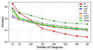
(a) painting$\rightarrow$real

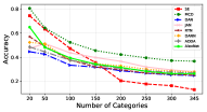
(b) infograph$\rightarrow$real

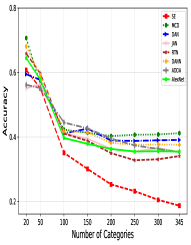
(c) sketch$\rightarrow$clipart

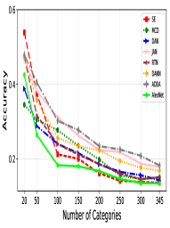
(d) quickdraw$\rightarrow$clipart

Figure 5: Accuracy vs. Number of Catogries. We plot how the performances of different models will change when the number of categories increases. We select four UDA settings, i.e., painting$\rightarrow$real, infograph$\rightarrow$real, sketch$\rightarrow$clipart, quickdraw$\rightarrow$clipart. The figure shows the performance of all models drop significantly with the increase of category number.

(a) DAN Features on SVHN

(b) M³SDA-$\beta$ Features on SVHN

(c) DAN Features on Caltech

(d) M³SDA-$\beta$ Features on Caltech

Figure 6: Feature visualization: t-SNE plot of DAN features and M³SDA-$\beta$ features on SVHN in mm,mt,up,sy$\rightarrow$sv setting; t-SNE of DAN features and M³SDA-$\beta$ features on Caltech in A,D,W$\rightarrow$C setting. We use different markers and different colors to denote different categories. (Best viewed in color.)

D Details of Digit Experiments

Network Architecture In our digital experiments (Table 2), our feature extractor is composed of three conv layers and two fc layers. We present the conv layers as (input, output, kernel, stride, padding) and fc layers as (input, output). The three conv layers are: conv1 (3, 64, 5, 1, 2), conv2 (64, 64, 5, 1, 2), conv3 (64, 128, 5, 1, 2). The two fc layers are: fc1 (8192, 3072), fc2 (3072, 2048). The architecture of the feature generator is: (conv1, bn1, relu1, pool1)-(conv2, bn2, relu2, pool2)-(conv3, bn3, relu3)-(fc1, bn4, relu4, dropout)-(fc2, bn5, relu5). The classifier is a single fc layer, i.e. fc3 (2048, 10).

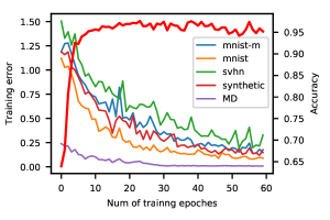
Figure 7: Analysis: training error of each classifier, Moment Discrepancy (MD, defined in Equation 1), and accuracy (red bold line) w.r.t. training epochs in mm,mt,sv,sy$\rightarrow$up setting. The bold red line shows how the accuracy changes w.r.t. training epochs.

Convergence Analysis As our framework involves multiple classifiers and the model is trained with multiple losses, we visualize the learning procedure of mm,mt,sv,sy$\rightarrow$up setting in Figure 7. The figure shows the training errors of multiple classifiers are decreasing, despite some frequent deviations. The MD (Moment Discrepancy) loss decreases in a steady way, demonstrating that the MD loss and the cross-entropy loss gradually converge.

E Feature visualization

To demonstrate the transfer ability of our model, we visualize the DAN [25] features and M³SDA-$\beta$ features with t-SNE embedding in two tasks: mm,mt,up,sy$\rightarrow$sv and A,D,W$\rightarrow$C. The results are shown in Figure 6. We make two important observations: i) Comparing Figure 6(a) with Figure 6(b), we find that M³SDA-$\beta$ is capable of learning more discriminative features; ii) From Figure 6(c) and Figure 6(d), we find that the clusters of M³SDA-$\beta$ features are more compact than those of DAN, which suggests that the features learned by M³SDA-$\beta$ attain more desirable discriminative property. These observations imply the superiority of our model over DAN in multi-source domain adaptation.

F Effect of Category Number

In this section, we show more results to clarify how the number of categories affects the performances of the state-of-the-art models. We choose the following four settings, i.e., painting$\rightarrow$real (Figure 5(a)), infograph$\rightarrow$real (Figure 5(b)), sketch$\rightarrow$clipart (Figure 5(c)), quickdraw$\rightarrow$clipart (Figure 5(d)), and gradually increase the number of categories from 20 to 345. From the four figures, we make the following interesting observations:

• All the models perform well when the number of categories is small. However, their performances drop rapidly when the number of categories increases.

• Self-Ensembling [7] model has a good performance when the number of categories is small, but it is not suitable to large scale domain adaptation.

G ResNet baselines

We report ResNet [13] source only baselines in Table 7. The MCD [38] and the SE [7] methods (In Table 3) are based on ResNet101 and ResNet152, respectively. We have observed these two methods both perform worse than their source only baselines, which indicates negative transfer [31] phenomenon occurs in these two scenarios. Exploring why negative transfer happens is beyond the scope of this literature. One preliminary guess is due to the large number of categories.

H Train/Test Split

We show the detailed number of images we used in our experiments in Table 8. For each domain, we follow a 70%/30% schema to split the dataset to training and testing trunk. The “Per-Class” row shows the average number of images that each category contains.

	clp	inf	pnt	qdr	rel	skt	Total
Train	34,019	37,087	52,867	120,750	122,563	49,115	416,401
Test	14,818	16,114	22,892	51,750	52,764	21,271	179,609
Total	48,837	53,201	75,759	172,500	175,327	70,386	596,010
Per-Class	141	154	219	500	508	204	1,728

Table 8: Train/Test split. We split DomainNet with a 70%/30% ratio. The “Per-Class” row shows the average number of images that each category contains.

I Image Samples

We sample the images for each domain and show them in Figure 9 (clipart), Figure 10 (infograph), Figure 11 (painting), Figure 12 (quickdraw), Figure 13 (real), and Figure 14 (sketch).

(a) Original

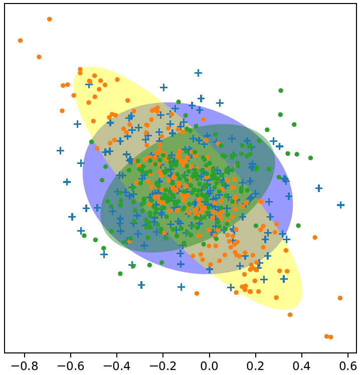
(b) No Within-Source Matching

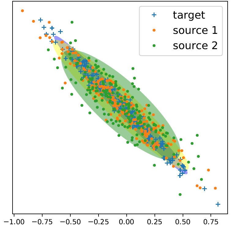
(c) Our model

Figure 8: Yellow and green points are sampled from two source domains. Blue points are sampled from target domain.

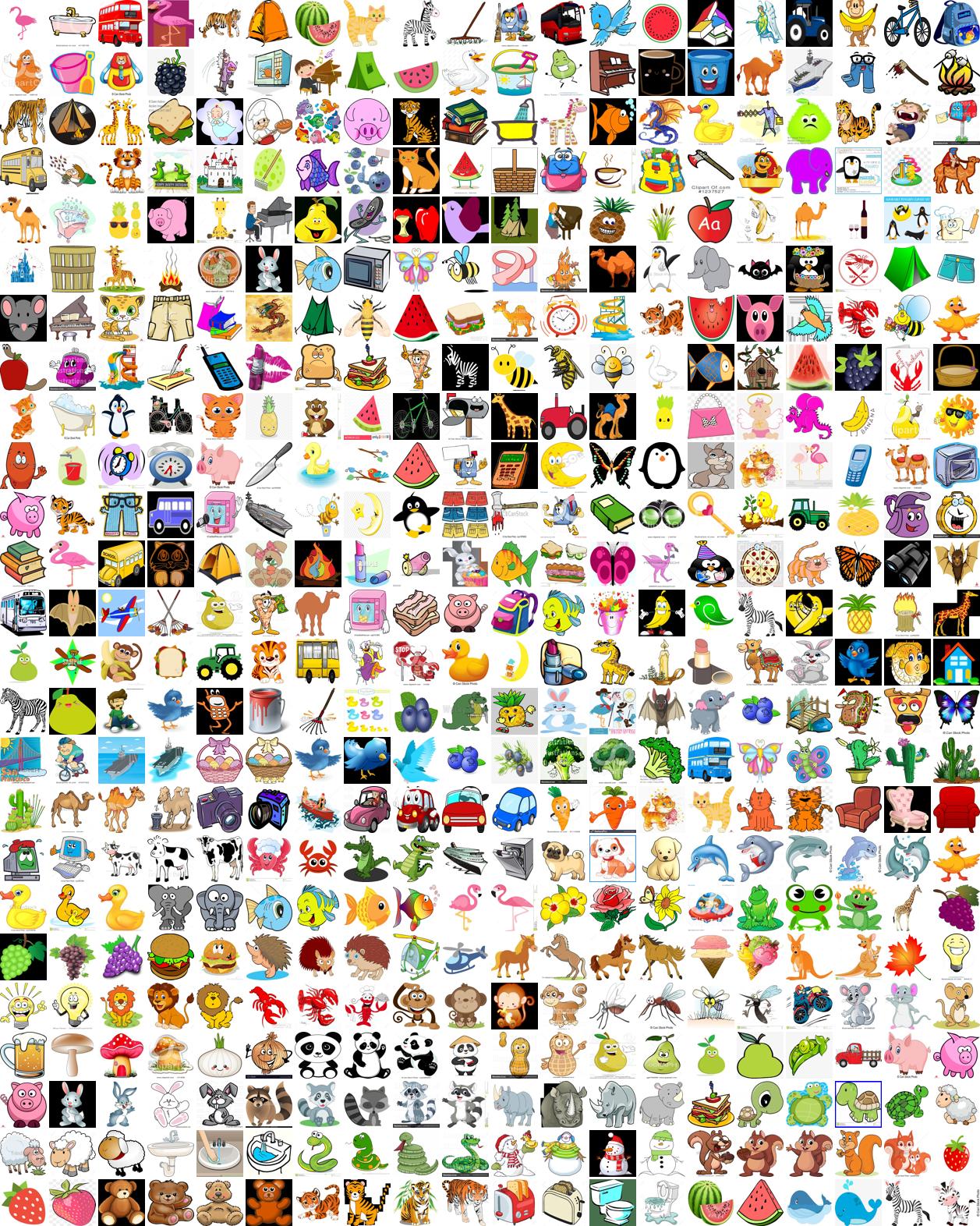
Figure 9: Images sampled from clipart domain of the DomainNet dataset.

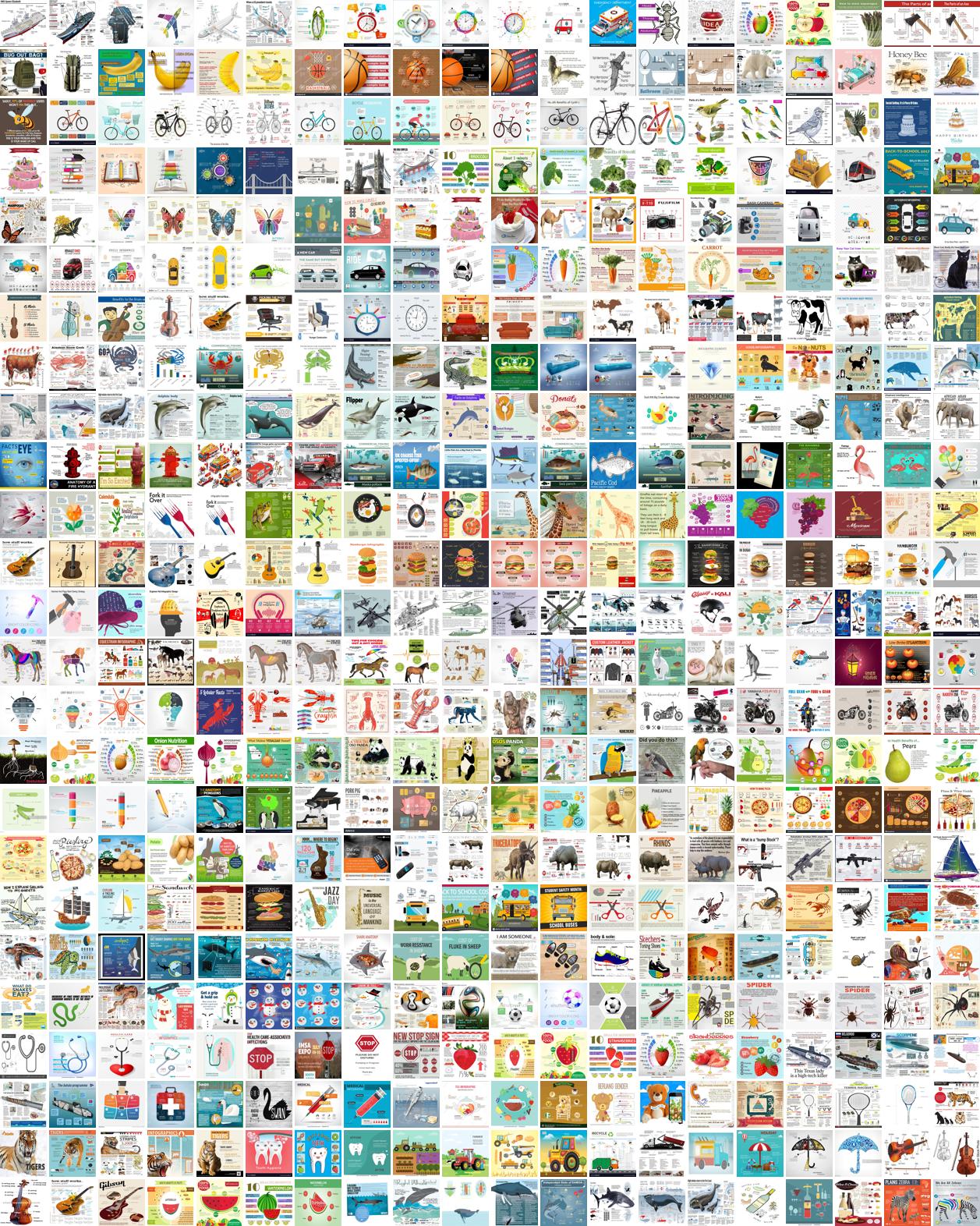
Figure 10: Images sampled from infograph domain of the DomainNet dataset.

Figure 11: Images sampled from painting domain of the DomainNet dataset.

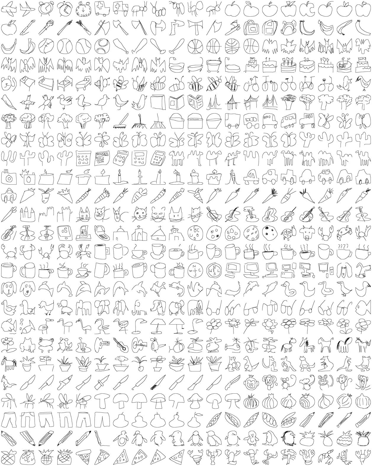
Figure 12: Images sampled from quickdraw domain of the DomainNet dataset.

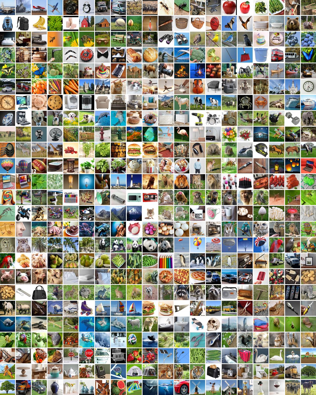
Figure 13: Images sampled from real domain of the DomainNet dataset.

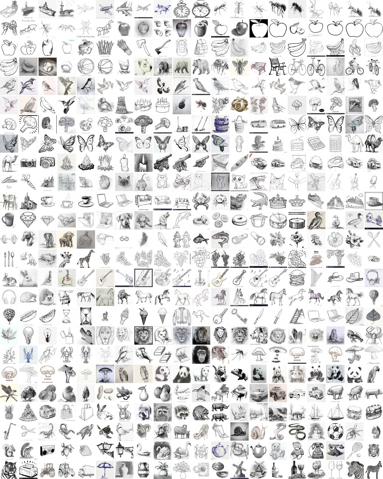
Figure 14: Images sampled from sketch domain of the DomainNet dataset.

J Dataset Statistics

Table 10, Table 11, and Table 12 show the detailed statistics of our DomainNet dataset. Our dataset contains 6 distinct domains, 345 categories and $\sim$0.6 million images. The categories are from 24 divisions, which are: Furniture, Mammal, Tool, Cloth, Electricity, Building, Office, Human Body, Road Transportation, Food, Nature, Cold Blooded, Music, Fruit, Sport, Tree, Bird, Vegetable, Shape, Kitchen, Water Transportation, Sky Transportation, Insect, Others.

K Toy Experiment

In multi-source domain adaptation, the source domains are not i.i.d and as a result, are not automatically aligned with each other. Intuitively, it is not possible to perfectly align the target domain with every source domain, if the source domains are not aligned themselves. More specifically, as explained in the paragraph following Theorem  1, the last term of our target error bound is lower bounded by pairwise divergences between source domains. This motivates our algorithm to also align the moments between each pair of source domains.

Empirically, let’s consider a toy experiment setting in which we have two source domains (denoted by yellow and green) and one target domain (denoted by blue), as shown in Figure 8. In the experiments, we utilize a 2-layer fully connected neural network as the backbone. We can observe the source domains and target domain are better aligned when matching source domain distributions using our model is applied.

L Time Consumption

We show the training and testing time consumption in Figure 9. The experiments are run in PyTorch with a NVIDIA TITAN X GPU on CentOS 7 server. The server has 8 Intel CORE i7 processors. We benchmark all the models with a minibatch size of 16 and an image size of 224 x 224. The CUDA version is 8.0 with CuDNN 5.15.

Models	Training (ms)	Testing (ms)
ResNet101	200.87	60.84
M3SDA	267.58	61.20

Table 9: Time consumption of our model and the baseline.

Furniture
class	clp	inf	pnt	qdr	rel	skt	total	class	clp	inf	pnt	qdr	rel	skt	total	class	clp	inf	pnt	qdr	rel	skt	total
bathtub	100	135	45	500	517	210	1507	bed	197	180	46	500	724	188	1835	bench	71	47	167	500	662	290	1737
ceiling fan	35	63	38	500	217	25	878	chair	94	148	53	500	320	96	1211	chandelier	223	29	57	500	393	34	1236
couch	232	61	26	500	601	60	1480	door	81	49	347	500	371	361	1709	dresser	41	23	141	500	234	13	952
fence	165	99	49	500	770	140	1723	fireplace	138	98	15	500	700	123	1574	floor lamp	180	100	10	500	246	278	1314
hot tub	144	86	197	500	757	49	1733	ladder	74	96	418	500	442	244	1774	lantern	179	58	218	500	526	40	1521
mailbox	18	45	101	500	595	151	1410	picture frame	88	60	372	500	207	115	1342	pillow	151	170	144	500	656	115	1736
postcard	91	37	88	500	636	49	1401	see saw	299	28	166	500	273	519	1785	sink	133	32	94	500	231	464	1454
sleeping bag	96	14	17	500	406	591	1624	stairs	386	282	27	500	353	525	2073	stove	256	255	16	500	614	269	1910
streetlight	326	113	537	500	463	268	2207	suitcase	377	224	187	500	432	309	2029	swing set	143	35	129	500	556	96	1459
table	297	736	104	500	563	300	2500	teapot	222	209	391	500	631	327	2280	toilet	175	519	31	500	583	118	1926
toothbrush	159	556	11	500	582	235	2043	toothpaste	105	468	31	500	511	198	1813	umbrella	145	511	299	500	362	297	2114
vase	161	319	262	500	632	187	2061	wine glass	220	628	168	500	338	245	2099
Mammal
bat	35	99	306	500	361	160	1461	bear	124	81	379	500	585	178	1847	camel	154	31	289	500	493	130	1597
cat	43	172	344	500	796	130	1985	cow	188	134	156	500	541	17	1536	dog	70	225	721	500	782	311	2609
dolphin	84	165	401	500	581	85	1816	elephant	115	188	425	500	789	266	2283	giraffe	134	172	105	500	594	186	1691
hedgehog	138	48	248	500	727	109	1770	horse	201	216	521	500	645	103	2186	kangaroo	106	60	214	500	613	122	1615
lion	46	64	505	500	516	330	1961	monkey	123	85	405	500	699	166	1978	mouse	74	50	445	500	147	127	1343
panda	87	86	264	500	587	79	1603	pig	93	203	326	500	577	227	1926	rabbit	105	135	269	500	695	94	1798
raccoon	187	24	249	500	676	348	1984	rhinoceros	102	91	220	500	684	183	1780	sheep	114	70	334	500	796	475	2289
squirrel	221	180	779	500	693	389	2762	tiger	315	285	422	500	607	386	2515	whale	343	432	357	500	671	272	2575
zebra	235	306	298	500	683	278	2300
Tool
anvil	122	23	152	500	332	91	1220	axe	48	92	219	500	382	219	1460	bandage	47	322	197	500	399	56	1521
basket	78	219	417	500	444	192	1850	boomerang	92	45	41	500	628	120	1426	bottlecap	118	26	538	500	606	139	1927
broom	171	35	84	500	639	234	1663	bucket	142	56	61	500	335	162	1256	compass	191	36	78	500	272	14	1091
drill	136	44	21	500	573	144	1418	dumbbell	387	86	189	500	581	190	1933	hammer	147	70	46	500	347	71	1181
key	59	68	97	500	229	137	1090	nail	41	256	838	500	674	23	2332	paint can	60	42	172	500	560	34	1368
passport	26	120	34	500	535	97	1312	pliers	38	65	293	500	453	163	1512	rake	119	66	58	500	594	93	1430
rifle	83	149	240	500	520	122	1614	saw	76	34	150	500	118	110	988	screwdriver	205	34	73	500	417	373	1602
shovel	214	17	112	500	450	630	1923	skateboard	263	50	152	500	557	419	1941	stethoscope	343	107	346	500	496	237	2029
stitches	206	285	17	500	207	34	1249	sword	139	124	470	500	591	384	2208	syringe	128	240	10	500	589	222	1689
wheel	133	385	19	500	410	166	1613
Cloth
belt	137	95	17	500	661	125	1535	bowtie	146	95	292	500	533	327	1893	bracelet	293	123	150	500	715	300	2081
camouflage	181	27	72	500	124	69	973	crown	208	17	81	500	170	176	1152	diamond	207	109	17	500	577	117	1527
eyeglasses	201	118	83	500	680	219	1801	flip flops	147	53	206	500	525	120	1551	hat	120	201	400	500	529	77	1827
helmet	163	263	27	500	622	210	1785	jacket	72	82	272	500	457	84	1467	lipstick	101	104	196	500	446	110	1457
necklace	83	115	347	500	697	114	1856	pants	16	173	381	500	398	136	1604	purse	41	119	49	500	544	228	1481
rollerskates	204	49	322	500	493	141	1709	shoe	127	291	260	500	587	645	2410	shorts	140	29	161	500	443	529	1802
sock	167	453	31	500	531	453	2135	sweater	222	92	153	500	579	167	1713	t-shirt	98	320	12	500	367	155	1452
underwear	253	354	12	500	286	132	1537	wristwatch	285	470	18	500	553	224	2050
Electricity
calculator	55	28	12	500	374	69	1038	camera	58	66	156	500	480	109	1369	cell phone	38	170	136	500	520	23	1387
computer	287	97	19	500	362	31	1296	cooler	214	21	13	500	528	90	1366	dishwasher	109	47	107	500	508	40	1311
fan	148	49	16	500	460	66	1239	flashlight	221	62	418	500	461	95	1757	headphones	285	224	181	500	551	188	1929
keyboard	32	95	370	500	503	64	1564	laptop	26	118	161	500	387	319	1511	light bulb	12	185	482	500	262	405	1846
megaphone	73	91	160	500	560	189	1573	microphone	143	70	152	500	562	156	1583	microwave	16	114	10	500	338	170	1148
oven	14	59	11	500	492	176	1252	power outlet	25	76	102	500	620	95	1418	radio	30	101	65	500	398	165	1259
remote control	117	70	111	500	554	47	1399	spreadsheet	187	397	34	500	751	677	2546	stereo	289	334	12	500	211	90	1436
telephone	148	279	78	500	479	255	1739	television	136	546	51	500	400	127	1760	toaster	196	337	107	500	536	267	1943
washing machine	265	519	15	500	466	155	1920

Table 10: Detailed statistics of the DomainNet dataset.

Building
class	clp	inf	pnt	qdr	rel	skt	total	class	clp	inf	pnt	qdr	rel	skt	total	class	clp	inf	pnt	qdr	rel	skt	total
The Eiffel Tower	114	190	321	500	553	276	1954	The Great Wall	116	80	159	500	530	148	1533	barn	157	150	426	500	313	201	1747
bridge	66	61	471	500	769	335	2202	castle	47	123	225	500	682	56	1633	church	54	20	142	500	668	35	1419
diving board	182	12	127	500	593	71	1485	garden	63	291	213	500	815	98	1980	garden hose	147	48	179	500	534	84	1492
golf club	207	169	650	500	552	695	2773	hospital	95	48	50	500	674	24	1391	house	108	306	105	500	374	144	1537
jail	104	26	54	500	587	94	1365	lighthouse	123	66	411	500	722	384	2206	pond	105	72	603	500	777	95	2152
pool	139	173	90	500	680	103	1685	skyscraper	195	159	179	500	284	466	1783	square	163	211	144	500	98	727	1843
tent	153	234	141	500	590	339	1957	waterslide	159	328	12	500	606	115	1720	windmill	245	372	397	500	635	245	2394
Office
alarm clock	93	23	84	500	521	202	1423	backpack	33	341	265	500	439	220	1798	bandage	47	322	197	500	399	56	1521
binoculars	246	55	148	500	402	266	1617	book	167	188	65	500	731	146	1797	calendar	66	54	44	500	176	59	899
candle	151	68	261	500	621	77	1678	clock	69	50	266	500	619	44	1548	coffee cup	357	191	185	500	643	33	1909
crayon	141	41	19	500	512	285	1498	cup	128	52	582	500	406	396	2064	envelope	147	60	291	500	665	183	1846
eraser	138	34	17	500	356	51	1096	map	42	206	423	500	507	193	1871	marker	57	44	103	500	336	240	1280
mug	168	41	500	500	598	186	1993	nail	41	256	838	500	674	23	2332	paintbrush	25	28	365	500	413	75	1406
paper clip	122	25	112	500	549	119	1427	pencil	51	369	183	500	461	26	1590	scissors	205	103	65	500	568	437	1878
Human Body
arm	50	129	422	500	235	249	1585	beard	156	93	373	500	728	481	2331	brain	76	283	233	500	724	270	2086
ear	101	58	187	500	348	199	1393	elbow	199	74	97	500	398	155	1423	eye	108	168	292	500	695	489	2252
face	54	110	20	500	696	452	1832	finger	153	71	57	500	625	283	1689	foot	85	111	86	500	558	261	1601
goatee	255	236	129	500	562	219	1901	hand	97	268	262	500	563	264	1954	knee	45	56	130	500	505	273	1509
leg	89	174	178	500	659	145	1745	moustache	222	28	430	500	424	107	1711	mouth	110	103	51	500	457	172	1393
nose	57	226	512	500	362	103	1760	skull	178	29	189	500	329	600	1825	smiley face	113	46	77	500	226	441	1403
toe	85	407	12	500	356	78	1438	tooth	101	473	109	500	257	181	1621
Road Transportation
ambulance	80	20	74	500	623	115	1412	bicycle	71	272	196	500	705	343	2087	bulldozer	111	55	58	500	635	199	1558
bus	101	183	112	500	745	233	1874	car	99	356	45	500	564	145	1709	firetruck	167	39	359	500	562	328	1955
motorbike	42	209	106	500	772	209	1838	pickup truck	46	116	143	500	619	188	1612	police car	104	51	87	500	740	119	1601
roller coaster	143	46	75	500	637	61	1462	school bus	230	142	66	500	478	405	1821	tractor	154	316	183	500	636	263	2052
train	109	373	406	500	681	240	2309	truck	117	678	158	500	673	265	2391	van	207	806	12	500	442	138	2105
Food
birthday cake	165	69	119	500	307	233	1393	bread	197	232	315	500	794	276	2314	cake	108	140	172	500	786	77	1783
cookie	97	78	54	500	677	33	1439	donut	139	65	373	500	630	127	1834	hamburger	187	210	147	500	559	185	1788
hot dog	38	138	148	500	644	143	1611	ice cream	160	187	311	500	657	184	1999	lollipop	74	28	252	500	607	106	1567
peanut	84	60	82	500	423	130	1279	pizza	77	157	127	500	600	202	1663	popsicle	288	79	171	500	639	117	1794
sandwich	189	110	139	500	579	132	1649	steak	155	360	50	500	758	238	2061
Nature
beach	105	183	499	500	622	79	1988	cloud	172	142	278	500	324	100	1516	hurricane	92	68	133	500	420	99	1312
lightning	171	68	199	500	560	94	1592	moon	126	195	324	500	568	155	1868	mountain	67	57	319	500	791	195	1929
ocean	54	47	475	500	591	77	1744	rain	71	78	352	500	274	235	1510	rainbow	61	44	84	500	231	46	966
river	134	155	558	500	651	111	2109	snowflake	175	41	405	500	66	460	1647	star	111	204	98	500	61	205	1179
sun	248	352	572	500	161	258	2091	tornado	169	329	373	500	497	211	2079
Cold Blooded
crab	108	50	153	500	717	152	1680	crocodile	164	56	120	500	713	161	1714	fish	130	195	429	500	479	373	2106
frog	163	118	167	500	761	203	1912	lobster	243	47	254	500	649	174	1867	octopus	190	49	331	500	726	149	1945
scorpion	171	53	133	500	447	455	1759	sea turtle	236	190	410	500	621	254	2211	shark	203	279	269	500	183	532	1966
snail	166	18	321	500	465	405	1875	snake	168	57	425	500	501	470	2121	spider	161	154	308	500	593	645	2361
Music
cello	93	34	158	500	450	64	1299	clarinet	214	25	89	500	407	33	1268	drums	194	18	205	500	769	214	1900
guitar	103	204	203	500	632	183	1825	harp	258	37	224	500	649	45	1713	piano	20	66	296	500	570	119	1571
saxophone	236	74	358	500	482	310	1960	trombone	227	195	175	500	484	191	1772	trumpet	117	247	122	500	391	188	1565
violin	174	282	203	500	512	203	1874

Table 11: Detailed statistics of the DomainNet dataset.

Fruit
class	clp	inf	pnt	qdr	rel	skt	total	class	clp	inf	pnt	qdr	rel	skt	total	class	clp	inf	pnt	qdr	rel	skt	total
apple	88	75	445	500	54	181	1343	banana	50	376	359	500	258	204	1747	blackberry	106	214	14	500	568	60	1462
blueberry	171	110	167	500	733	129	1810	grapes	93	171	318	500	734	287	2103	pear	74	115	448	500	438	183	1758
pineapple	83	139	333	500	673	131	1859	strawberry	357	308	530	500	454	198	2347	watermelon	193	401	410	500	671	128	2303
Sport
baseball	116	369	122	500	87	48	1242	baseball bat	106	353	145	500	118	196	1418	basketball	61	219	276	500	237	160	1453
flying saucer	233	40	242	500	396	137	1548	hockey puck	188	59	236	500	400	95	1478	hockey stick	155	197	194	500	394	119	1559
snorkel	278	81	179	500	689	397	2124	soccer ball	85	163	268	500	272	377	1665	tennis racquet	187	195	18	500	456	202	1558
yoga	165	447	161	500	371	251	1895
Tree
bush	46	12	67	500	31	626	1282	cactus	119	36	122	500	658	61	1496	flower	253	140	485	500	360	336	2074
grass	148	312	332	500	378	173	1843	house plant	25	292	416	500	484	156	1873	leaf	12	96	504	500	414	378	1904
palm tree	65	277	607	500	333	166	1948	tree	126	511	571	500	536	555	2799
Bird
bird	336	208	222	500	803	306	2375	duck	142	51	419	500	404	276	1792	flamingo	274	39	224	500	542	142	1721
owl	133	114	496	500	757	202	2202	parrot	75	62	336	500	781	266	2020	penguin	121	201	447	500	700	209	2178
swan	469	52	507	500	326	236	2090
Vegetable
asparagus	49	134	408	500	659	209	1959	broccoli	105	229	100	500	679	181	1794	carrot	52	251	265	500	565	34	1667
mushroom	136	298	254	500	788	252	2228	onion	87	62	471	500	599	158	1877	peas	90	120	90	500	680	81	1561
potato	86	61	58	500	608	83	1396	string bean	139	87	70	500	491	68	1355
Shape
circle	199	248	292	500	259	202	1700	hexagon	196	362	160	500	592	116	1926	line	13	210	502	500	102	25	1352
octagon	29	115	19	500	465	117	1245	squiggle	148	115	674	500	71	442	1950	triangle	183	364	298	500	376	303	2024
zigzag	323	412	110	500	515	144	2004
Kitchen
fork	200	63	84	500	351	176	1374	frying pan	187	68	169	500	399	132	1455	hourglass	100	100	206	500	289	134	1329
knife	32	108	30	500	582	129	1381	lighter	66	27	27	500	587	118	1325	matches	60	19	56	500	333	56	1024
spoon	228	127	158	500	534	406	1953	wine bottle	230	442	59	500	407	274	1912
Water Transportation
aircraft carrier	27	88	133	500	390	63	1201	canoe	68	71	395	500	703	129	1866	cruise ship	208	94	223	500	632	158	1815
sailboat	162	119	322	500	422	361	1886	speedboat	271	76	141	500	620	487	2095	submarine	344	183	550	500	607	207	2391
Sky Transportation
airplane	73	62	212	500	218	331	1396	helicopter	145	216	257	500	804	200	2122	hot air balloon	198	48	453	500	732	170	2101
parachute	82	60	140	500	629	233	1644
Insect
ant	81	62	235	500	381	111	1370	bee	202	233	313	500	452	144	1844	butterfly	160	162	387	500	658	249	2116
mosquito	56	232	65	500	562	144	1559
Others
The Mona Lisa	150	112	191	500	289	145	1387	angel	165	17	504	500	31	299	1516	animal migration	235	68	604	500	444	112	1963
campfire	122	53	217	500	489	86	1467	cannon	103	14	54	500	300	93	1064	dragon	105	30	231	500	485	196	1547
feather	268	432	344	500	505	336	2385	fire hydrant	149	59	29	500	579	148	1464	mermaid	207	30	99	500	449	228	1513
snowman	174	123	901	500	114	712	2524	stop sign	169	54	87	500	168	109	1087	teddy-bear	124	407	301	500	528	238	2098
traffic light	211	280	60	500	379	127	1557

Table 12: Detailed statistics of the DomainNet dataset.

References

- [1] Shai Ben-David, John Blitzer, Koby Crammer, Alex Kulesza, Fernando Pereira, and Jennifer Wortman Vaughan. A theory of learning from different domains. Machine learning, 79(1-2):151–175, 2010.
- [2] Shai Ben-David, John Blitzer, Koby Crammer, Fernando Pereira, et al. Analysis of representations for domain adaptation. Advances in neural information processing systems, pages 137–144, 2007.
- [3] Konstantinos Bousmalis, George Trigeorgis, Nathan Silberman, Dilip Krishnan, and Dumitru Erhan. Domain separation networks. In Advances in Neural Information Processing Systems, pages 343–351, 2016.
- [4] Koby Crammer, Michael Kearns, and Jennifer Wortman. Learning from multiple sources. Journal of Machine Learning Research, 9(Aug):1757–1774, 2008.
- [5] Carl De Boor, Carl De Boor, Etats-Unis Mathématicien, Carl De Boor, and Carl De Boor. A practical guide to splines, volume 27. Springer-Verlag New York, 1978.
- [6] Lixin Duan, Dong Xu, and Shih-Fu Chang. Exploiting web images for event recognition in consumer videos: A multiple source domain adaptation approach. In Computer Vision and Pattern Recognition (CVPR), 2012 IEEE Conference on, pages 1338–1345. IEEE, 2012.
- [7] Geoff French, Michal Mackiewicz, and Mark Fisher. Self-ensembling for visual domain adaptation. In International Conference on Learning Representations, 2018.
- [8] Yaroslav Ganin and Victor Lempitsky. Unsupervised domain adaptation by backpropagation. In Francis Bach and David Blei, editors, Proceedings of the 32nd International Conference on Machine Learning, volume 37 of Proceedings of Machine Learning Research, pages 1180–1189, Lille, France, 07–09 Jul 2015. PMLR.
- [9] Muhammad Ghifary, W Bastiaan Kleijn, and Mengjie Zhang. Domain adaptive neural networks for object recognition. In Pacific Rim international conference on artificial intelligence, pages 898–904. Springer, 2014.
- [10] Muhammad Ghifary, W Bastiaan Kleijn, Mengjie Zhang, David Balduzzi, and Wen Li. Deep reconstruction-classification networks for unsupervised domain adaptation. In European Conference on Computer Vision, pages 597–613. Springer, 2016.
- [11] Boqing Gong, Yuan Shi, Fei Sha, and Kristen Grauman. Geodesic flow kernel for unsupervised domain adaptation. In Computer Vision and Pattern Recognition (CVPR), 2012 IEEE Conference on, pages 2066–2073. IEEE, 2012.
- [12] Arthur Gretton, Karsten M Borgwardt, Malte Rasch, Bernhard Schölkopf, and Alex J Smola. A kernel method for the two-sample-problem. In Advances in neural information processing systems, pages 513–520, 2007.
- [13] Kaiming He, Xiangyu Zhang, Shaoqing Ren, and Jian Sun. Deep residual learning for image recognition. In Proceedings of the IEEE conference on computer vision and pattern recognition, pages 770–778, 2016.
- [14] Judy Hoffman, Mehryar Mohri, and Ningshan Zhang. Algorithms and theory for multiple-source adaptation. In S. Bengio, H. Wallach, H. Larochelle, K. Grauman, N. Cesa-Bianchi, and R. Garnett, editors, Advances in Neural Information Processing Systems 31, pages 8246–8256. Curran Associates, Inc., 2018.
- [15] Judy Hoffman, Eric Tzeng, Taesung Park, Jun-Yan Zhu, Phillip Isola, Kate Saenko, Alexei Efros, and Trevor Darrell. CyCADA: Cycle-consistent adversarial domain adaptation. In Jennifer Dy and Andreas Krause, editors, Proceedings of the 35th International Conference on Machine Learning, volume 80 of Proceedings of Machine Learning Research, pages 1989–1998, Stockholmsmässan, Stockholm Sweden, 10–15 Jul 2018. PMLR.
- [16] Taeksoo Kim, Moonsu Cha, Hyunsoo Kim, Jung Kwon Lee, and Jiwon Kim. Learning to discover cross-domain relations with generative adversarial networks. In Doina Precup and Yee Whye Teh, editors, Proceedings of the 34th International Conference on Machine Learning, volume 70 of Proceedings of Machine Learning Research, pages 1857–1865, International Convention Centre, Sydney, Australia, 06–11 Aug 2017. PMLR.
- [17] Piotr Koniusz, Yusuf Tas, Hongguang Zhang, Mehrtash Harandi, Fatih Porikli, and Rui Zhang. Museum exhibit identification challenge for the supervised domain adaptation and beyond. In The European Conference on Computer Vision (ECCV), September 2018.
- [18] Alex Krizhevsky, Ilya Sutskever, and Geoffrey E Hinton. Imagenet classification with deep convolutional neural networks. In Advances in neural information processing systems, pages 1097–1105, 2012.
- [19] Yann LeCun, Léon Bottou, Yoshua Bengio, and Patrick Haffner. Gradient-based learning applied to document recognition. Proceedings of the IEEE, 86(11):2278–2324, 1998.
- [20] Chun-Liang Li, Wei-Cheng Chang, Yu Cheng, Yiming Yang, and Barnabás Póczos. Mmd gan: Towards deeper understanding of moment matching network. In Advances in Neural Information Processing Systems, pages 2203–2213, 2017.
- [21] Da Li, Yongxin Yang, Yi-Zhe Song, and Timothy Hospedales. Deeper, broader and artier domain generalization. In International Conference on Computer Vision, 2017.
- [22] Yujia Li, Kevin Swersky, and Rich Zemel. Generative moment matching networks. In International Conference on Machine Learning, pages 1718–1727, 2015.
- [23] Ming-Yu Liu, Thomas Breuel, and Jan Kautz. Unsupervised image-to-image translation networks. In Advances in Neural Information Processing Systems, pages 700–708, 2017.
- [24] Ming-Yu Liu and Oncel Tuzel. Coupled generative adversarial networks. In Advances in neural information processing systems, pages 469–477, 2016.
- [25] Mingsheng Long, Yue Cao, Jianmin Wang, and Michael Jordan. Learning transferable features with deep adaptation networks. In Francis Bach and David Blei, editors, Proceedings of the 32nd International Conference on Machine Learning, volume 37 of Proceedings of Machine Learning Research, pages 97–105, Lille, France, 07–09 Jul 2015. PMLR.
- [26] Mingsheng Long, Han Zhu, Jianmin Wang, and Michael I Jordan. Unsupervised domain adaptation with residual transfer networks. In Advances in Neural Information Processing Systems, pages 136–144, 2016.
- [27] Mingsheng Long, Han Zhu, Jianmin Wang, and Michael I. Jordan. Deep transfer learning with joint adaptation networks. In Proceedings of the 34th International Conference on Machine Learning, ICML 2017, Sydney, NSW, Australia, 6-11 August 2017, pages 2208–2217, 2017.
- [28] Yishay Mansour, Mehryar Mohri, Afshin Rostamizadeh, and A R. Domain adaptation with multiple sources. In D. Koller, D. Schuurmans, Y. Bengio, and L. Bottou, editors, Advances in Neural Information Processing Systems 21, pages 1041–1048. Curran Associates, Inc., 2009.
- [29] Youssef Mroueh, Tom Sercu, and Vaibhava Goel. McGan: Mean and covariance feature matching GAN. In Doina Precup and Yee Whye Teh, editors, Proceedings of the 34th International Conference on Machine Learning, volume 70 of Proceedings of Machine Learning Research, pages 2527–2535, International Convention Centre, Sydney, Australia, 06–11 Aug 2017. PMLR.
- [30] OA Muradyan and S Ya Khavinson. Absolute values of the coefficients of the polynomials in weierstrass’s approximation theorem. Mathematical notes of the Academy of Sciences of the USSR, 22(2):641–645, 1977.
- [31] Sinno Jialin Pan and Qiang Yang. A survey on transfer learning. IEEE Transactions on knowledge and data engineering, 22(10):1345–1359, 2010.
- [32] Xingchao Peng and Kate Saenko. Synthetic to real adaptation with generative correlation alignment networks. In 2018 IEEE Winter Conference on Applications of Computer Vision, WACV 2018, Lake Tahoe, NV, USA, March 12-15, 2018, pages 1982–1991, 2018.
- [33] Xingchao Peng, Baochen Sun, Karim Ali, and Kate Saenko. Learning deep object detectors from 3d models. In Proceedings of the IEEE International Conference on Computer Vision, pages 1278–1286, 2015.
- [34] Xingchao Peng, Ben Usman, Neela Kaushik, Judy Hoffman, Dequan Wang, and Kate Saenko. Visda: The visual domain adaptation challenge. arXiv preprint arXiv:1710.06924, 2017.
- [35] Xingchao Peng, Ben Usman, Kuniaki Saito, Neela Kaushik, Judy Hoffman, and Kate Saenko. Syn2real: A new benchmark forsynthetic-to-real visual domain adaptation. CoRR, abs/1806.09755, 2018.
- [36] Joaquin Quionero-Candela, Masashi Sugiyama, Anton Schwaighofer, and Neil D. Lawrence. Dataset Shift in Machine Learning. The MIT Press, 2009.
- [37] Kate Saenko, Brian Kulis, Mario Fritz, and Trevor Darrell. Adapting visual category models to new domains. In European conference on computer vision, pages 213–226. Springer, 2010.
- [38] Kuniaki Saito, Kohei Watanabe, Yoshitaka Ushiku, and Tatsuya Harada. Maximum classifier discrepancy for unsupervised domain adaptation. In The IEEE Conference on Computer Vision and Pattern Recognition (CVPR), June 2018.
- [39] Baochen Sun, Jiashi Feng, and Kate Saenko. Return of frustratingly easy domain adaptation. In AAAI, volume 6, page 8, 2016.
- [40] Eric Tzeng, Judy Hoffman, Kate Saenko, and Trevor Darrell. Adversarial discriminative domain adaptation. In Computer Vision and Pattern Recognition (CVPR), volume 1, page 4, 2017.
- [41] Eric Tzeng, Judy Hoffman, Ning Zhang, Kate Saenko, and Trevor Darrell. Deep domain confusion: Maximizing for domain invariance. arXiv preprint arXiv:1412.3474, 2014.
- [42] Vladimir N Vapnik and A Ya Chervonenkis. On the uniform convergence of relative frequencies of events to their probabilities. In Measures of complexity, pages 11–30. Springer, 2015.
- [43] Hemanth Venkateswara, Jose Eusebio, Shayok Chakraborty, and Sethuraman Panchanathan. Deep hashing network for unsupervised domain adaptation. In (IEEE) Conference on Computer Vision and Pattern Recognition (CVPR), 2017.
- [44] Jindong Wang, Wenjie Feng, Yiqiang Chen, Han Yu, Meiyu Huang, and Philip S Yu. Visual domain adaptation with manifold embedded distribution alignment. In ACM Multimedia Conference, 2018.
- [45] Ruijia Xu, Ziliang Chen, Wangmeng Zuo, Junjie Yan, and Liang Lin. Deep cocktail network: Multi-source unsupervised domain adaptation with category shift. In Proceedings of the IEEE Conference on Computer Vision and Pattern Recognition, pages 3964–3973, 2018.
- [46] Zili Yi, Hao (Richard) Zhang, Ping Tan, and Minglun Gong. Dualgan: Unsupervised dual learning for image-to-image translation. In ICCV, pages 2868–2876, 2017.
- [47] Werner Zellinger, Thomas Grubinger, Edwin Lughofer, Thomas Natschläger, and Susanne Saminger-Platz. Central moment discrepancy (CMD) for domain-invariant representation learning. CoRR, abs/1702.08811, 2017.
- [48] Zhen Zhang, Mianzhi Wang, Yan Huang, and Arye Nehorai. Aligning infinite-dimensional covariance matrices in reproducing kernel hilbert spaces for domain adaptation. In Proceedings of the IEEE Conference on Computer Vision and Pattern Recognition, pages 3437–3445, 2018.
- [49] Han Zhao, Shanghang Zhang, Guanhang Wu, José MF Moura, Joao P Costeira, and Geoffrey J Gordon. Adversarial multiple source domain adaptation. In Advances in Neural Information Processing Systems, pages 8568–8579, 2018.
- [50] Jun-Yan Zhu, Taesung Park, Phillip Isola, and Alexei A Efros. Unpaired image-to-image translation using cycle-consistent adversarial networks. In Computer Vision (ICCV), 2017 IEEE International Conference on, 2017.
- [51] Fuzhen Zhuang, Xiaohu Cheng, Ping Luo, Sinno Jialin Pan, and Qing He. Supervised representation learning: Transfer learning with deep autoencoders. In IJCAI, pages 4119–4125, 2015.