Boltzmann Generators – Sampling Equilibrium States of Many-Body Systems with Deep Learning

$1$: FU Berlin, Department of Mathematics and Computer Science, Arnimallee 6, 14195 Berlin, Germany

$2$: FU Berlin, Department of Physics, Arnimallee 14, 14195 Berlin, Germany

$3$: Rice University, Department of Chemistry, Houston, Texas 77005, United States

$4$: Tongji University, School of Mathematical Sciences, Shanghai, 200092, P.R. China

$\dagger$: Equal contribution

*: Correspondence to: frank.noe@fu-berlin.de

Abstract: Computing equilibrium states in condensed-matter many-body systems, such as solvated proteins, is a long-standing challenge. Lacking methods for generating statistically independent equilibrium samples in “one shot”, vast computational effort is invested for simulating these system in small steps, e.g., using Molecular Dynamics. Combining deep learning and statistical mechanics, we here develop Boltzmann Generators, that are shown to generate unbiased one-shot equilibrium samples of representative condensed matter systems and proteins. Boltzmann Generators use neural networks to learn a coordinate transformation of the complex configurational equilibrium distribution to a distribution that can be easily sampled. Accurate computation of free energy differences and discovery of new configurations are demonstrated, providing a statistical mechanics tool that can avoid rare events during sampling without prior knowledge of reaction coordinates.

Introduction

Statistical mechanics is concerned with computing the average behavior of many copies of a physical system based on its microscopic constituents and their interactions. For example, what is the average magnetization in an Ising model of interacting magnetic spins, or what is the probability of a protein to be folded as a function of the temperature? Under a wide range of conditions, the equilibrium probability of a microscopic configuration $\mathbf{x}$ (setting of all spins, positions of all protein atoms, etc.) is proportional to $\mathrm{e}^{-u(\mathbf{x})}$, for example, the well-known Boltzmann distribution. The dimensionless energy $u(\mathbf{x})$ contains the potential energy of the system, the temperature and optionally other thermodynamic quantities.

Except for simple model systems, we presently have no approach to directly draw “one-shot”, i.e., statistically independent, samples $\mathbf{x}$ from Boltzmann-type distributions in order to compute statistics of the system, such as free energy differences. Therefore, one currently relies on trajectory methods, such as Markov-Chain Monte Carlo (MCMC) or Molecular Dynamics (MD) simulations that make tiny changes to $\mathbf{x}$ in each step. These methods sample from the Boltzmann distribution in the long run, but many simulation steps are needed to produce a statistically independent sample. This is because complex systems often have metastable (long-lived) phases or states and the transitions between them are rare events – for example, $10^{9}-10^{15}$ MD simulation steps are needed to fold or unfold a protein. As a result, MCMC and MD methods are extremely expensive and consume much of the worldwide supercomputing resources.

A common approach to enhance sampling is to speed up rare events by biasing user-defined order parameters, or “reaction coordinates”, that may be of mechanical  (?, ?, ?, ?), thermodynamic  (?, ?, ?), or alchemical nature  (?, ?). Applying these techniques to high-dimensional systems with a priori unknown transition mechanisms is challenging, as identifying suitable order parameters and avoiding rare events in other, unbiased directions, becomes extremely difficult. For example, the development of enhanced simulation protocols for the binding of small drug molecules to proteins has become a research area in its own right  (?).

Here we set out to develop a “Boltzmann Generator” machine that is trained on a given energy function $u(\mathbf{x})$ and then produces unbiased one-shot samples from $\mathrm{e}^{-u(\mathbf{x})}$, circumventing the sampling problem without requiring any knowledge of reaction coordinates. At first sight, this enterprise seems hopeless for condensed-matter systems and complex polymers (Fig. 3a, Fig. 5b,c). In these systems, strongly repulsive particles are densely packed, such that the number of low-energy configurations are vanishingly few compared to the number of possible ways to place particles.

Key to the solution is combining the strengths of deep machine learning  (?) and statistical mechanics (Fig. 1a): We train a deep invertible neural network, to learn a coordinate transformation from $\mathbf{x}$ to a so-called “latent” representation $\mathbf{z}$, in which the low-energy configurations of different states are close to each other and can be easily sampled, e.g. using a Gaussian normal distribution. Enhancing MD sampling by user-defined coordinate transformations has been proposed previously  (?). The novelty of Boltzmann Generators is that this transformation is learned, and owing to the deep transformation network, can be as complicated as needed to represent state changes in the many-body system. As Boltzmann Generators are invertible, every sample $\mathbf{z}$ can be back-transformed to a configuration $\mathbf{x}$ with high Boltzmann probability. We can improve the ability to find relevant parts of configuration space by “learning from example”, where the potential energy $u(\mathbf{x})$ used to train the Boltzmann Generator is complemented by relevant samples $\mathbf{x}$, e.g., from the folded or unfolded state of a protein, but without knowing the probabilities of these states. Then we employ statistical mechanics which offers a rich set of tools to generate the target distribution $\mathrm{e}^{-u(\mathbf{x})}$ when the proposal distribution is sufficiently similar.

This paper demonstrates that Boltzmann Generators can be trained to generate low-energy structures of condensed-matter systems and protein molecules in one shot, as shown for model systems and a millisecond-timescale conformational change of the BPTI protein. When the Boltzmann Generator is initialized with a few structures from different metastable states, it can generate statistically independent samples from these states and can compute the free energy profiles of the corresponding transitions without suffering from rare events. Although Boltzmann Generators do not require reaction coordinates, they can be included in the training in order to sample continuous free energy profiles and low-probability states. When trained in this way, Boltzmann Generators can also generate physically realistic transition pathways by performing simple linear interpolations in latent space. We also show that multiple independent Boltzmann Generators, trained on disconnected MD or MCMC simulations of different states, can be employed to compute free energy differences between these states in a direct and inexpensive way and without requiring any reaction coordinates. Finally, we demonstrate that when employing established sampling methods such as Metropolis Monte Carlo in the latent space of a Boltzmann Generator, efficient methods can be constructed to find new states and gradually explore state space.

Boltzmann Generators

Neural networks that can draw statistically independent samples from a desired distribution are called directed generative networks  (?, ?). Such networks have been demonstrated to generate photorealistic images  (?), to produce deceivingly realistic speech audio  (?), and even to sample formulae of chemical compounds with certain physico-chemical properties  (?). In these domains, the exact target distribution is not known and the network is “trained by example” using large databases of images, audio or molecules. Here we are in the inverse situation, as we can compute the Boltzmann weight of each generated sample $\mathbf{x}$, but we do not have samples from the Boltzmann distribution a priori. The idea of Boltzmann Generators is as follows (Fig. 1a):

1. We learn a neural network transformation $F_{zx}$ such that when sampling $\mathbf{z}$ from a simple prior, e.g., a Gaussian normal distribution, $F_{zx}(\mathbf{z})$ will provide a configuration $\mathbf{x}$ which has a high Boltzmann weight, i.e. is coming from a distribution $p_{X}(\mathbf{x})$ that is similar to the target Boltzmann distribution.

2. To obtain an unbiased sample and compute Boltzmann-weighted averages, we reweight the generated distribution $p_{X}(\mathbf{x})$ to the Boltzmann distribution $\mathrm{e}^{-u(\mathbf{x})}$. This can be achieved with various algorithms; here the simplest one is used: assign the statistical weight $w(\mathbf{x})=\mathrm{e}^{-u(\mathbf{x})}/p_{X}(\mathbf{x})$ to every sample $\mathbf{x}$ and then compute desired statistics, such as free energy differences using this weight.

Figure 1: Boltzmann Generators. a) A Boltzmann Generator is trained by minimizing the difference between its generated distribution and the desired Boltzmann distribution. Generation proceeds by drawing “latent” space samples $\mathbf{z}$ from a simple prior distribution (e.g., Gaussian) and transforming them to configurations $\mathbf{x}$. The variable transformation is formed by stacking invertible transformations $f_{1},...,f_{n}$ to a deep neural network $F_{zx}$ and its inverse, $F_{xz}$. To compute thermodynamics, such as configurational free energies, the samples must be reweighted to the Boltzmann distribution. b) The Boltzmann Generator is composed of invertible neural network blocks. Here, a non-volume-preserving transformation block is shown as an example.

For both, training and reweighting, it is important that we can compute the probability $p_{X}(\mathbf{x})$ of generating a configuration $\mathbf{x}$. This can be achieved when $F_{zx}$ is an invertible transformation, which allows us to transform the known prior distribution $p_{Z}(\mathbf{z})$ to $p_{X}(\mathbf{x})$ (Fig. 1a, Methods)  (?, ?). Physically, invertible transformations are analogous to flows of a fluid that transform the probability density from configuration space to latent space, or backwards. Volume-preserving transformations, comparable to incompressible fluids were introduced in  (?). Here we employ the non-volume preserving transformations introduced in  (?) (Fig. 1b), as they allow the probability distribution to be scaled differently at different parts of configuration space. Alternatively, Boltzmann Generators can be built using more general invertible transformations  (?, ?, ?). Invertibility is achieved by adopting special neural network architectures (Fig. 1b; Methods). Multiple trainable invertible “blocks” can be stacked, thus encoding complicated variable transformations in the form of a deep invertible neural network (Fig. 1a).

Boltzmann Generators are trained by combining two modes: training by energy and training by example. Training by energy is the main principle behind Boltzmann Generators, and proceeds as follows: We sample random vectors $\mathbf{z}$ from a Gaussian prior distribution, and then transform them through the neural network to proposal configurations, $\mathbf{x}=F_{zx}(\mathbf{z})$. In this way, the Boltzmann Generator will generate configurations from a proposal distribution $p_{X}(\mathbf{x})$, which, initially will be very different from the Boltzmann distribution, and include configurations with very high energies. Next we compute the difference between the generated distribution $p_{X}(\mathbf{x})$ from the Boltzmann distribution whose statistical weights $\mathrm{e}^{-u(\mathbf{x})}$ are known. For Boltzmann Generators, a natural measure of this difference is the relative entropy, or Kullback-Leibler (KL) divergence. The KL divergence can be computed as the following expectation value over samples $\mathbf{z}$ (Methods):

$$J_{KL}=\mathbb{E}_{\mathbf{z}}\left[u(F_{zx}(\mathbf{z}))-\log R_{zx}(\mathbf{z})\right]$$ (1)

Here, $u(F_{zx}(\mathbf{z}))$ is the energy of the generated configuration. $R_{zx}$ is the determinant of the Boltzmann Generator’s Jacobian matrix, and measures how much the network scales the configuration space volume at $\mathbf{z}$. The invertible network layers are designed such that $R_{zx}$ can be easily computed (Methods). We treat $J_{KL}$ as a loss function: In order to train the Boltzmann Generator, we approximate $J_{KL}$ using a batch of around 1000 samples, and then change the neural network parameters so as to decrease $J_{KL}$. A few hundred or thousand such iterations are required to train the Boltzmann Generator for the examples in this paper. The resulting few million computations of the potential energy in Eq. (1) are the main computational investment and take between one minute and few hours for the present systems.

The KL divergence (1) is equivalent to the free energy difference of transforming the Gaussian prior distribution to the generated distribution (Methods, Supp. Mat.): The first term $\mathbb{E}\left[u(F_{zx}(\mathbf{z}))\right]$ is the mean potential energy, i.e. the internal energy of the system. The second term $\mathbb{E}\left[\log R_{zx}(\mathbf{z})\right]$ is equal to the entropic contribution to the free energy at the chosen temperature, plus a constant factor. The terms in Eq. (1) counter-play in an interesting way: the first term tries to minimize the energy, and therefore trains the Boltzmann Generator to sample low-energy structures. The second term tries to maximize the entropy of the generated distribution, and therefore prevents the Boltzmann Generator from the so-called mode-collapse  (?), i.e. the repetitive sampling of a single minimum-energy configuration which would minimize the first term.

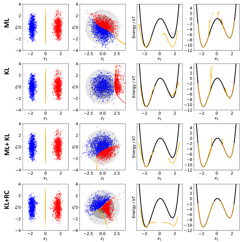
Figure S2: Different training methods for Boltzmann Generators using the double well example (Fig. 2). Columns show: (1) distribution in configuration space $\mathbf{x}$, (2) distribution in latent space $\mathbf{z}$, (3) free energy of Boltzmann Generator output $p_{X}(\mathbf{x})$ along $x_{1}$, (4) free energy after reweighting, vertical bars show uncertainties (one standard deviation, 68% percentile). Training proceeds by 200 iterations of ML and then 500 iterations of the method given in the rows, using equal weights for these modes. Training by example (ML) only reproduces the distribution of the training data, which can be reweighted to the Boltzmann distribution in this low-dimensional example but reweighting from the ML-generated distribution fails for high-dimensional examples. Training by energy (KL) alone tends to collapse to a single metastable state. ML+KL combined samples closer to the Boltzmann distribution than ML and avoids metastable state collapse, but samples high-energy transition states with low probability. KL+RC performs best in this example.

Despite the entropy term in Eq. (1), training by energy alone is not sufficient as it tends to focus sampling on the most stable metastable state (Fig. S2). We therefore additionally employ training by example, which is the standard training method used in other machine learning applications, and is here implemented with the maximum likelihood principle. We initialize the Boltzmann Generator with some “valid” configurations $\mathbf{x}$, e.g., from short initial MD simulations or an experimental structure, transform them to latent space via $\mathbf{z}=F_{xz}(\mathbf{x})$. Maximizing their likelihood in the Gaussian distribution corresponds to minimizing the loss function  (?, ?):

$$J_{ML}=\mathbb{E}_{\mathbf{x}}\left[\frac{1}{2}\left\|F_{xz}(\mathbf{x})\right\|^{2}-\log R_{xz}(\mathbf{x})\right].$$ (2)

Here, the first term $\frac{1}{2}\left\|F_{xz}(\mathbf{x})\right\|^{2}$ is the energy of a harmonic oscillator corresponding to the Gaussian prior distribution. Training by example is especially used in the early stages of training, as it helps $F_{zx}$ to focus on relevant parts of state space.

By combining training by energy and training by example, we can sample configurations that have high probabilities and low free energies. However, sometimes we want to sample states with low equilibrium probabilities, such as transition states along a certain reaction coordinate (RC) whose free energy profile is of interest. For this purpose, we introduce an RC loss that can optionally be used to enhance the sampling of a Boltzmann Generator along a chosen RC (Methods).

Results

Illustration on model systems

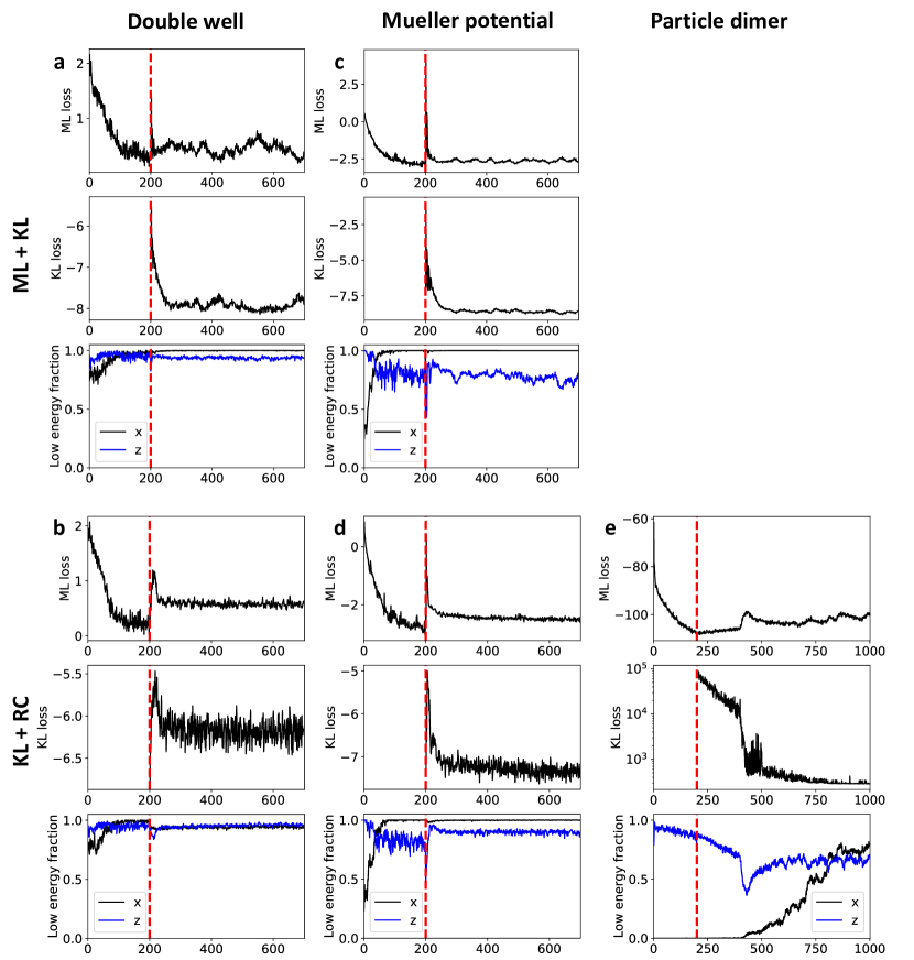
Figure S1: Convergence metrics for Boltzmann Generators reported in Fig. 2 and Fig. 3. Boltzmann Generators were trained with by energy and example (top row), or by energy and using a reaction coordinate loss (bottom row). Panels show: ML loss $J_{ML}$ (top), KL loss $J_{KL}$ (middle) and the low-energy fractions in configuration space $\mathbf{x}$ and in latent space $\mathbf{z}$ (bottom). These are defined by the fraction of Boltzmann Generator samples ($\mathbf{z}\rightarrow\mathbf{x}$) whose configuration energies are within the 99% percentile of the energies of the input data, and the fraction of input data that when mapped to latent space ($\mathbf{x}\rightarrow\mathbf{z}$) are within the 99% percentile of the energy distribution of a harmonic oscillator with the respective dimension. a-b): Double well potential. c-d): Mueller potential. e) Solvated particle dimer.

We first illustrate Boltzmann Generators using two-dimensional model potentials that have metastable states separated by high energy barriers: the double well potential, and the Mueller potential (Fig. 2a,g). MD simulations stay in one metastable state for a long time before a rare transition event occurs. Hence, the distributions in configuration space $(x_{1},x_{2})$ are split into two modes (Fig. 2a,g, transition state and intermediate state ensembles are shown in yellow for clarity but are not used for training). We are training Boltzmann Generators using the two short and disconnected simulations whose samples are shown in Fig. 2a,g (details in Supp. Mat., convergence in Fig. S1). Fig. 2b,h show the latent spaces learned by the Boltzmann Generator, note that their exact appearance varies between different runs due to stochasticity in neural network training. In both latent spaces, the probability densities of the two states and the transition/intermediate states are “repacked” so as to form a density concentrated around the origin.

We use the Boltzmann generators by sampling from their latent spaces according to Gaussian distributions. After transforming these variables via $F_{zx}$, this produces uncorrelated and low-energy samples from both stable states without any sampling problem (Fig. 2c-d,i-j) . A variety of training methods succeed in sampling across the barrier such that the rare event nature of the system is eliminated (Fig. S2). Using a Boltzmann Generator trained by energy and by example with simple reweighting reproduces the precise free energy differences of the two metastable states, although no reaction coordinate is employed to indicate the direction of the rare event (Fig. 2e,k; green). By additionally training with the RC loss to promote sampling along $x_{1}$ (double well) or $x_{2}$ (Mueller potential), the low-probability transition states are sampled (Fig. 2d,j;, orange), and the full free energy profile can be reconstructed with high precision (Fig. 2e,k; orange).

The Boltzmann Generator repacks the high-probability regions of configuration space into a concentrated latent space density. We therefore ask about the physical interpretation of direct paths in latent space. Specifically, we interpolate linearly between the latent space representations of samples from different energy minima, similar as it is done with generative networks in other disciplines  (?, ?). When mapping these linear interpolations back to configuration space, they result in nonlinear pathways that have low-energies and high probabilities (Fig. 2f,l). Although there is no general guarantee that linear paths in latent space will result in low energies, this result indicates that the latent spaces learned by Boltzmann Generators can be used to provide candidates of order parameters for bias-enhanced or path-based sampling methods  (?, ?, ?).

For the double-well system, the unbiased MD simulation needs on average $4\cdot 10^{6}$ MD steps for a single return trip between the two states (Supp. Mat.), and about $100$ such crossings are required to compute the free energy difference with the same precision as the Boltzmann Generator results shown in (Fig. 2e). The total effort of training the Boltzmann Generator (including generating the initial simulation data) corresponds to about $10^{6}$ steps, but once this is done, statistically independent samples can be generated at no significant cost. For this simple system, the Boltzmann Generator is therefore about a factor $100$ more efficient than direct simulation, but much more extreme savings can be observed for complex systems, as shown below.

Figure 2: Application of Boltzmann Generators on two-dimensional bistable systems. a,g) Two-dimensional potentials: double well ($x_{1}$ is the slow coordinate) and Mueller potential. Two short MD simulation trajectories (blue, red) stay in their metastable states without crossing. Transition state and intermediate state ensembles are shown (orange) but not used for training. b,h) Latent-space distribution of trajectories shown in a,g) when mapped through trained $F_{xz}$. c,i) potential energy distribution sampled by MD simulation (grey) and by Boltzmann Generators trained by energy and by example (KL+ML, green) and using reaction coordinate training (KL+RC, orange). d,j) Boltzmann Generator sample distribution along the slow coordinates. For the Mueller potential, $x_{\mathrm{proj}}$ is defined as projection along the vector $(1,-1)$. e,k) Free energy estimates obtained from Boltzmann Generator samples after reweighting. f,l) Paths generated by linear interpolation in Boltzmann Generator latent space (b,h) between random pairs of “blue” and “red” MD samples.

Thermodynamics of condensed-matter systems

As a second example, we demonstrate that Boltzmann Generators can sample high-probability structures and efficiently compute the thermodynamics in crowded condensed matter systems. We simulated a dense system of two-dimensional particles confined to a box as suggested in  (?) (Fig. 3a). Immersed in the fluid is a bistable particle dimer whose open and closed states are separated by a high barrier (Fig. 3b). Opening or closing the dimer directly is not possible due to the high density of the system, but requires concerted rearrangement of solvent particles. At close distances, particles repel each other strongly, resulting in a crowded system. Thus, the fraction of low-energy configurations is vanishingly small, and manually designing a sampling method that simultaneously places all $38$ particles and achieves low energies appears unfeasible.

We train a Boltzmann Generator to sample one-shot low-energy configurations and use it in order to compute the free energy profiles of opening / closing the dimer. Key to treat explicit-solvent systems such as this one is to incorporate the permutation invariance of solvent molecules. If physically identical solvent molecules would be distinguished, every exchange of solvent molecule positions due to diffusion would represent a new configuration, resulting in an enormous configuration space even for this 38-particle system. We therefore remove identical-particle permutations from all configurations input into or sampled by the Boltzmann Generator by exchanging particle labels so as to minimize the distance to a reference configuration (Supp. Mat.).

The training is initialized with examples from separate, disconnected simulations of the open and closed states, but in later stages, training by energy (1) dominates (Supp. Mat., Fig. S1, Table S1). The trained Boltzmann Generator has learned a transformation of the complex configuration space density to a concentrated, 76-dimensional ball in latent space (Fig. 3c). Indeed, direct sampling from a 76-dimensional Gaussian in latent space and transformation via $F_{zx}$ generates configurations where all particles are placed without significant clashes, and potential energies that overlap with the energy distribution of the unbiased MD trajectories (Fig. 3d). Also, realistic transition states that have not been included in any training data are sampled (Fig. 3d, middle).

To demonstrate the computation of thermodynamic quantities, we perform training by energy (1) simultaneously to a range of temperatures (Supp. Mat.). While the temperature changes the configuration space distribution in a complex way it can be modeled as a simple scaling factor in the width of the Gaussian prior distribution (Methods). Then, we sample the Boltzmann Generator for a range of temperatures and use simple reweighting to compute the free energies along the dimer distances. As shown in Fig. 3e, these temperature-dependent free energies agree precisely with extensive umbrella sampling simulations that employ bias potentials along the dimer distance ( (?), Supp. Mat.).

We estimate that the MD simulation needs at least $10^{12}$ steps to spontaneously sample a single transition from closed to open state and back (Supp. Mat.), and about $100$ such transitions would be needed to compute free energy differences with the precision of Boltzmann Generators shown in Fig. 3e. The total effort to train the Boltzmann Generator is about $3\cdot 10^{7}$ energy evaluations, but then statistically independent samples can be drawn in one shot at the entire temperature range trained at, resulting in at least $7$ orders of magnitude speedup compared to MD.

As above, we perform linear interpolations between the latent space representations of open- and closed-dimer samples. A significant fraction of all pair interpolations result in low-energy pathways. The lowest-energy interpolation of 100 randomly selected pairs of end-states is shown in Fig. 3f, representing a physically meaningful rearrangement of the dimer and solvent.

Figure 3: Repulsive particle System with bistable dimer. a) Closed (blue) and open (red) configurations from MD simulations (input data). b) Bistable dimer potential. c) Distribution of MD simulation data in latent space coordinates $z_{1},z_{2}$ after training Boltzmann Generator. d) Potential energy distribution from MD (grey) and Boltzmann generator for closed (blue), open (red) and transition configurations (yellow). Insets show one-shot Boltzmann Generator samples. e) Free energy differences as a function of dimer distance and relative temperature sampled with Boltzmann generators (generation and reweighting, green bullets with intervals indicating one standard error from 10 independent repeats) and umbrella sampling (black lines). f) Linear latent space interpolation between the the closed and open structures shown in top row.

Exploring configuration space

In the previous examples, Boltzmann Generators were used to sample known regions of configuration space and compute statistics thereof. Here, we demonstrate that Boltzmann Generators can help to explore configuration space. The basic idea is as follows: we construct an exploratory sampling method by employing an established sampling algorithm in latent space, while simultaneously training the Boltzmann Generator transformation using the configurations found so far.

We initialize the method with a (possibly small) set of configurations $X$. Training is done here by minimizing the symmetric loss function $J=J_{KL}+J_{ML}$ (Eq. 1-2). The likelihood loss function $J_{ML}$ is initially biased by the input data, but as $X$ approaches an unbiased Boltzmann sample, the symmetric loss converges to a meaningful distance of probabilities (Methods). As an example, we here use Metropolis Monte Carlo in the latent space Boltzmann Generator to update $X$ (Methods). The step-size is chosen adaptively but reaches the order of the latent space distribution width. Thus, large-scale configuration transitions in physical space can be overcome in a single Monte Carlo step.

We now revisit the three previous examples and initialize $X$ with only a single input configuration from the most stable state (Fig. 4a, d, g). The exploration method quickly fills the local metastable states, and finds new metastable states within a few $10^{5}$ energy calls, i.e., orders of magnitude faster than direct MD (Fig. 4b, e, h). This demonstrates that Boltzmann Generators sample new, previously unseen states with a significant probability, and that this ability can be turned into exploring configuration space when past samples are stored and reused for training.

The Metropolis Monte Carlo method causes the sample to converge towards the Boltzmann distribution. However, we do not need to wait for this method to be converged, as with sufficient samples in the states of interest, the equilibrium free energies can be computed by employing reweighting as in Figs. 2-3 above. While new states are found, the data-based loss $J_{ML}$ may increase and decrease again, while the Boltzmann Generator transformation is updated to include these new states (Fig. 4c, f, i; top row). During training, the energy-based loss $J_{KL}$ decreases steadily until the full Boltzmann distribution is sampled (Fig. 4c, f, i; middle row). We also observe that the Metropolis Monte Carlo efficiency, defined by the product of step-length and acceptance rate, tends to increase over time, although it may decrease temporarily when more states are found (Fig. 4c, f, i; top row).

Due to the invertible transformation between latent and configuration space, any sampling method that involves reweighting or Monte Carlo acceptance steps can be reformulated in Boltzmann Generator latent space, and potentially yield enhanced performance.

Figure 4: Exploration with Boltzmann Generators from a single snapshot. a-c) Double-well potential, d-f) Mueller potential, g-h) solvated particle dimer. a, d, g) Starting configuration. c, f, i) Convergence of the loss terms ($J_{ML}$ and $J_{KL}$) and the MCMC efficiency (product of step length and acceptance rate). b, e, h) Evolution of sample distribution over MCMC iteration. As soon as sufficient density is available in the states of interest, these distributions can be reweighted to equilibrium as in Figs. 2-3.

Complex molecules

We demonstrate that Boltzmann Generators can generate equilibrium all-atom structures of macromolecules in one shot using the Bovine Pancreatic Trypsin Inhibitor protein (BPTI) in an implicit solvent model (Fig. 5, Supp. Mat.). In order to train Boltzmann Generators for complex molecular models, we wrapped the energy and force computation functions of the OpenMM simulation software  (?) in the standard deep learning library Tensorflow  (?).

Training a Boltzmann Generator directly on the Cartesian coordinates resulted in large energies, and unrealistic structures with distorted bond lengths and angles. This problem was solved by incorporating the following coordinate transformation in the first layer of the Boltzmann Generator that is invertible up to rotation and translation of the molecule (Fig. 5a, Methods): the coordinates are split into Cartesian and internal coordinate sets. The Cartesian coordinates include heavy atoms of the backbone and the disulfide bridges. Cartesian coordinates are whitened, i.e. decorrelated and normalized, using a principal component analysis of the input data. During whitening, the six degrees of freedom corresponding to global translation and rotation of the molecule are discarded. The remaining side-chain atoms are measured in internal coordinates (bond-lengths, angles and torsions with respect to parent atoms), and subsequently normalized.

After this coordinate transformation, the learning problem is substantially simplified as the transformed input data are already nearly Gaussian distributed. We first demonstrate that Boltzmann Generators can learn to sample heterogeneous equilibrium structures when trained with examples from different configurations. To this end, we generated six short simulations of 20 nanoseconds each, starting from snapshots of the well-known 1-millisecond simulation of BPTI produced on the Anton supercomputer  (?). In the more common situation that no ultra-long MD trajectory is available, the Boltzmann Generator can be seeded with different crystallographic structures or homology models. In order to promote simultaneous sampling of high- and low-probability configurations, we included an RC loss using two slow collective coordinates that have been used earlier in the analysis of this BPTI simulation (Supp. Mat.),  (?, ?). Boltzmann Generators without use of reaction coordinates are discussed in the subsequent section.

Indeed, a trained Boltzmann Generator with 8 invertible blocks can sample all 892 atom positions (2676 dimensions) in one shot and produce locally and globally valid structures (Fig. 5c). The potential energies of samples exhibit significant overlap with the potential energy distribution of MD simulations (Fig. 5d), thus samples can be reweighted for free energy calculations. The probability distributions of most bond lengths and valence angles is almost indistinguishable from the distributions of the equilibrium MD simulations (Fig. 5e). The only exception is that the distributions of valence angles involving sulfur atoms is slightly narrower.

The trained Boltzmann Generator learns to encode and sample significantly different structures (Fig. 5f). In particular, it generates independent one-shot samples of the near-crystallographic structure “X” (1.4 ï¿œ mean backbone RMSD to crystal structure), and the open “O” structure which involves significant changes in flexible loops and repacking of side-chains (Fig. 5g,h). The X$\rightarrow$O transition has been sampled only once in the millisecond Anton trajectory, which is consistent with the observation of a millisecond-timescale “major-minor” state transition observed in nuclear magnetic resonance (NMR) spectroscopy  (?). We note that X$\leftrightarrow$O transition states are not included in the Boltzmann Generator training data.

Sampling such a transition and collecting statistics for it is challenging for any existing simulation method. Brute force MD simulations would require several milliseconds of simulation data. To employ enhanced sampling, an order parameter or reaction coordinate able to drive the complex rearrangement shown in Fig. 5g-h would need to be found, but since BPTI has multiple states with lifetimes on the order of 10-100 microseconds  (?, ?), the simulation time required for convergence would still be extensive. The computation of free energy differences using Boltzmann Generators will be discussed in the next section.

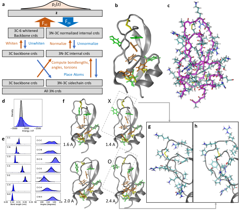
Figure 5: One-shot sampling of all-atom structures in different conformations of the BPTI protein. a) Boltzmann Generator for macromolecules: Backbone atoms are whitened using principal component analysis, side chain atoms are described in normalized internal coordinates. b) BPTI X-ray crystal structure (PDB: 5PTI). Cysteine disulfide bridges and aromatic residues are shown for orientation. c) One-shot Boltzmann Generator sample of all 892 atoms (2670 dimensions) of the BPTI protein similar to the X-ray structure. d) Potential energy distribution from MD simulation (grey) and Boltzmann generator one-shot samples (blue). e) Distribution of bonds and angles compared between MD simulation (black) and Boltzmann Generator (blue). f) Representative snapshots of four clusters of structures generated with the Boltzmann Generator. Backbone root mean square deviation RMSDs from the X-ray structure is given below structure (in ï¿œngstrï¿œm). Marked are the X-ray like structure “X” and the open structure “O”. g,h) Zoom into the most variable parts of the Boltzmann-generated samples from the “X” and “O” states. Side-chains are shown in atomistic resolution.

Thermodynamics between disconnected states

We develop a reaction-coordinate free approach to compute free energy differences from disconnected MD or MCMC simulations in separated states, such as two conformations of a protein. As demonstrated above, this can be achieved by a single Boltzmann Generator that simultaneously captures multiple metastable states and maps them to the same latent space $Z$, where they are connected via the Gaussian prior distribution (Fig. 2b,h, Fig. 3c). However, a more direct statistical mechanics idea that has been successfully applied to certain simple liquids and solids is to compute free energy differences by relating to a tractable reference state, e.g., ideal gas or crystal  (?, ?, ?). Here we show that Boltzmann Generators can turn this idea into a general method applicable to complex many-body systems.

Recall that the value of the energy loss function $J_{KL}$ (Eq. 1) estimates the free energy difference of transforming the Gaussian prior distribution to the generated distribution in configuration space. If we are now given MD data sampled in two or more disconnected states, we can train independent Boltzmann Generators for each of them. The goal here is not to explore configuration space, so training by energy is combined with training by example (Eq. 2) in order to restrain the generated distribution around the separate states. For each Boltzmann Generator, the transformation free energy is computed, e.g., $\langle J_{KL}^{1}\rangle$ and $\langle J_{KL}^{2}\rangle$, by sampling from the Gaussian prior distributions and inserting into (1). The free energy difference between the two states is directly given as a difference between these two values, $\Delta A_{12}=\langle J_{KL}^{2}\rangle-\langle J_{KL}^{1}\rangle$ (Fig. 6a).

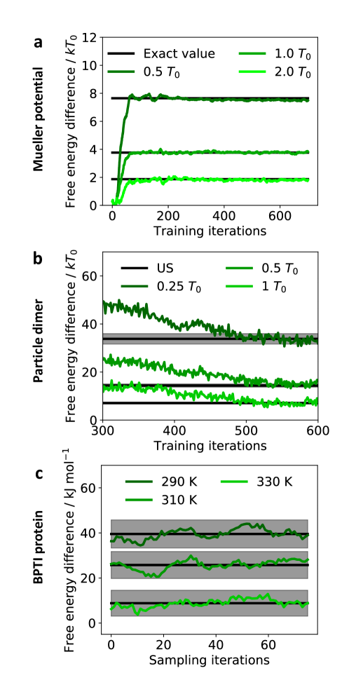
Figure S3: Convergence of free energy differences shown in Fig. 6. a) Mueller potential. b) Solvated Particle dimer. Convergence is shown for the last two training cycles, as the free energies are far from converged in earlier stages. References are from umbrella sampling, with intervals showing one standard error from 3 repeats. c) BPTI protein. For better performance, the free energy differences were not estimated during the training schedule reported in the Supp. Mat. Instead 75 training iterations were appended afterwards, and in each iteration 1000 samples of $J_{KL}$ were obtained at each temperature for free energy estimation. Black lines / grey intervals show the mean and one standard error estimates from this phase using 5 independent repeats.

We illustrate our method by computing temperature-dependent free energy differences for the four systems discussed above, each using two completely disconnected MD simulations as input. Since the estimate of the free energy difference is readily available from the value of the loss function, it can be conveniently tracked for convergence while the Boltzmann Generators are trained (Fig. 6b, Fig. S3).

For the two-dimensional systems (double well, Mueller potential) exact reference values for the free energy differences can be computed, and the Boltzmann Generator method recovers them accurately with a small statistical uncertainty over the entire temperature range (Fig. 6c, d), using tenfold less simulation data and about tenfold shorter training time than for the estimates using a single joint Boltzmann Generator reported in Fig. 2 (Supp. Mat.).

For the solvated bistable dimer, we use simulations that are tenfold shorter than for the single joint Boltzmann Generator reported in Fig. 3 and train two independent Boltzmann Generators at multiple temperatures. As a reference, three independent umbrella sampling simulations were conducted at each of five different temperatures. Both predictions of the free energy difference between open and closed dimer states are consistent and have overall similar uncertainties (Fig. 6e, Fig. S3b, note that the uncertainty of umbrella sampling is strongly temperature dependent). Although Umbrella Sampling is well-suited for this system with a clear reaction coordinate, the two-Boltzmann-Generator method required 50 times less energy calls than the Umbrella Sampling simulations at five temperatures, and yet makes predictions across the full temperature range (Supp. Mat.).

Finally, we use the same method to predict the temperature-dependent free energy difference of the “X” and “O” states in the BPTI protein. Sampling this millisecond transition ten times by brute-force MD would take around 30 years on one of the GTX1080 graphics cards that are used for computations in this paper, and would only give us the free-energy difference at a single temperature. While speeding up this complex transition with enhanced sampling may be possible, engineering a suitable order parameter is a time-consuming trial and error task. Training two Boltzmann Generators does not require any notion of reaction coordinate.

Here we use the two-Boltzmann-Generator method starting from two simulations of 20 ns each, that were here started from selected frames of the one-millisecond trajectory, but could generally be started from crystallographic structures or homology models. Conducting the MD simulations, training and analyzing the Boltzmann Generators used a total of less than $3\times 10^{7}$ energy calls, which results in a converged free energy estimate within a total of about 10 GPU hours, i.e. about 5 orders of magnitude faster than the brute-force approach (Fig. 6f, Fig. S3c). While no reference for this free energy difference in the given simulation model is known, the temperature profile admits basic consistency checks: The X-ray structure is identified as the most stable structure at temperatures below 330 K. The internal energy and entropy terms of the free energy difference (Eq. 1), are both positive across all temperatures. Consequently, the free energy decreases at high temperatures as the entropic stabilization becomes stronger. A higher configurational entropy of the “O” state is consistent with its more open loop structure (compare Fig. 5g and h) and the higher degree of fluctuations in the “O” state observed by the analysis in  (?).

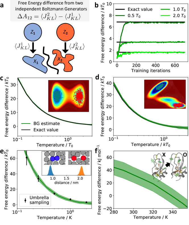
Figure 6: Thermodynamics between disconnected states by coupling multiple Boltzmann Generators. a) Using multiple Boltzmann Generators, we can compute free energy differences between states without requiring reaction coordinates, using only disconnected MD simulations in each of them. This is possible because each Boltzmann Generator estimates the free energy difference to a common reference state. b) Example for tracking convergence: estimate of free energy difference for the double well potential (multiple temperatures) as a function of the training iterations of two Boltzmann Generators. Convergence plots for the other systems are shown in Fig. S3. Results show estimates from two Boltzmann Generators with mean and one standard error computed from bootstrapping the converged segment of the free energy estimate. c) left-to-right transition in the double well, d) left-to-right transition in the Mueller potential, e) closed-to-open transition in the solvated bistable particle dimer, f) X$\rightarrow$O transition in an atomistic model of Bovine Pancreatic Trypsin Inhibitor (BPTI).

Discussion

Boltzmann Generators can overcome rare event sampling problems in many-body systems by generating independent samples from different metastable states in one shot. We have demonstrated this for dense and unstructured multi-body systems with up to 892 atoms (over 2600 dimensions) that are placed simultaneously, with most samples having globally and locally valid structures and potential energies in the range of the equilibrium distribution. In contrast to other generative neural networks, Boltzmann Generators produce unbiased samples, as the generated probability density is known at each sample point and can be reweighted to the target Boltzmann distribution. This feature directly translates into being able to compute free energy differences between different metastable states.

In contrast to enhanced sampling methods that directly operate in configuration space, such as Umbrella Sampling or Metadynamics, Boltzmann Generators can sample between metastable states without any pre-defined “reaction coordinate” connecting them. This is achieved by learning a coordinate transformation in which different metastable states become neighbors in the transformed space where the sampling occurs. If suitable reaction coordinates are known, these can be incorporated into the training in order to sample continuous pathways between states, e.g., to compute a continuous free energy profile along a reaction.

As in many areas of machine learning, key to success is to choose a representation of the input data which supports the learning problem. For macromolecules, we have found that a successful representation is to describe its backbone in Cartesian coordinates and all atoms that branch off from the backbone in internal coordinates. Additionally, normalizing these coordinates to mean zero and variance one already makes their probability distribution close to a Gaussian normal distribution, thus simplifying the learning problem considerably.

We have shown, in principle, how explicit solvent systems, can be treated. For this it is essential to build the physical invariances into the learning problem. Specifically, we need to account for permutation invariance: when two equivalent solvent molecules exchange positions, the potential energy of the system is unchanged, and so is the Boltzmann probability.

We have demonstrated scaling of Boltzmann Generators to 1000’s of dimensions. Generative networks in other fields have been able to generate photorealistic images with $10^{6}$ dimensions in one shot  (?). However, for the present application the statistical efficiency, i.e. the usefulness of these samples to compute equilibrium free energies, will decline with increasing dimension. Scaling to systems with 100,000’s of dimensions or more, such as solvated atomistic models of large proteins, can be achieved in different ways. Sampling of the full atomistic system may be approached by divide-and-conquer: In each iteration of such an approach, one would re-sample the positions of a cluster of atoms using the sum of potential energies between cluster atoms and all system atoms, and then, e.g., perform Monte Carlo steps using these cluster proposals. Alternatively, Boltzmann Generators could be used to sample lower-dimensional free energy surfaces learnt from all-atom models  (?).

A caveat of Boltzmann Generators is that, depending on the training method, they may not be ergodic, i.e. they may not be able to reach all configurations. Here we have proposed a training methods that promotes state space exploration by performing Monte Carlo steps in the Boltzmann Generator’s latent space while training the network. This may be viewed as a general recipe: The whole plethora of existing sampling algorithms, such as Umbrella Sampling, Metadynamics and replica exchange, can be reformulated in the latent space of a Boltzmann Generator, potentially leading to dramatic performance gains. Any such approach can always be combined with MD or MCMC moves in configuration space to ensure ergodicity.

Finally, the Boltzmann Generators described here learn a system-specific coordinate transformation. The approach would become much more general and efficient, if Boltzmann Generators could be pre-trained on certain building blocks of a molecular system, such as oligopeptides in solvent or a protein, and then re-used on a complex system consisting of these building blocks. A promising approach is to involve transferrable featurization methods developed in the context of machine learning for quantum mechanics  (?, ?).

In summary, Boltzmann Generators represent a powerful approach to address the long-standing rare-event sampling problem in many-body systems, and open the door for new developments in statistical mechanics.

Methods

A. Invertible networks

We employ invertible networks with trainable parameters $\boldsymbol{\theta}$ in order to learn the transformation between the Gaussian random variables $\mathbf{z}$ and the Boltzmann-distributed random variables $\mathbf{x}$:

$$\mathbf{z} =F_{xz}(\mathbf{x};\boldsymbol{\theta})$$

$$\mathbf{x} =F_{zx}(\mathbf{z};\boldsymbol{\theta}).$$

Hence $F_{xz}=F_{zx}^{-1}$. Each transformation has a Jacobian matrix with the pairwise first derivatives of outputs with respect to inputs:

$$\mathbf{J}_{zx}(\mathbf{z};\boldsymbol{\theta}) =\left[\frac{\partial F_{zx}(\mathbf{z};\boldsymbol{\theta})}{\partial z_{1}},...,\frac{\partial F_{zx}(\mathbf{z};\boldsymbol{\theta})}{\partial z_{n}}\right]$$

$$\mathbf{J}_{xz}(\mathbf{x};\boldsymbol{\theta}) =\left[\frac{dF_{xz}(\mathbf{x};\boldsymbol{\theta})}{dx_{1}},...,\frac{dF_{xz}(\mathbf{x};\boldsymbol{\theta})}{dx_{n}}\right]$$

The absolute value of the Jacobian’s determinant, $\left|\det\mathbf{J}_{zx}(\mathbf{z};\boldsymbol{\theta})\right|$, measures how much a volume element at $\mathbf{z}$ is scaled by the transformation. Below we will omit the symbol $\boldsymbol{\theta}$ and use the abbreviations:

$$R_{xz}(\mathbf{x}) =\left|\det\mathbf{J}_{xz}(\mathbf{x})\right|$$

$$R_{zx}(\mathbf{z}) =\left|\det\mathbf{J}_{zx}(\mathbf{z})\right|.$$

We use invertible transformations because they allow us to transform random variables as follows:

$$p_{X}(\mathbf{x}) =p_{Z}(\mathbf{z})R_{zx}(\mathbf{z})^{-1}=p_{Z}(F_{xz}(\mathbf{x}))R_{xz}(\mathbf{x})$$ (3)

$$p_{Z}(\mathbf{z}) =p_{X}(\mathbf{x})R_{xz}(\mathbf{x})^{-1}=p_{X}(F_{zx}(\mathbf{z}))R_{zx}(\mathbf{z})$$ (4)

Trainable invertible layers

We employ the RealNVP transformation as trainable part of invertible networks  (?). The main idea is to split the variables into two channels, $\mathbf{x}=(\mathbf{x}_{1},\mathbf{x}_{2})$, $\mathbf{z}=(\mathbf{z}_{1},\mathbf{z}_{2})$, and do only trivially invertible operations on each channel, such as multiplication and addition. Additionally, we use arbitrary, non-invertible artificial neural networks $S$ and $T$ are that respectively scale and translate the second input channel $\mathbf{x}_{2}$ using a nonlinear transformation of the first input channel $\mathbf{x}_{1}$.

$$f_{xz}(\mathbf{x}_{1},\mathbf{x}_{2}) : \begin{cases}\mathbf{z}_{1}=\mathbf{x}_{1}\\ \mathbf{z}_{2}=\mathbf{x}_{2}\odot\exp\left(S(\mathbf{x}_{1};\boldsymbol{\theta})\right)+T(\mathbf{x}_{1};\boldsymbol{\theta})\end{cases}$$ (5)

$$\log R_{xz} = \sum_{i}S_{i}(\mathbf{x}_{1};\boldsymbol{\theta})$$ (6)

$$f_{zx}(\mathbf{z}_{1},\mathbf{z}_{2}) : \begin{cases}\mathbf{x}_{1}=\mathbf{z}_{1}\\ \mathbf{x}_{2}=\left(\mathbf{z}_{2}-T(\mathbf{x}_{1};\boldsymbol{\theta})\right)\>\>\>\odot\exp\left(-S(\mathbf{z}_{1};\boldsymbol{\theta})\right)\end{cases}$$ (7)

$$\log R_{zx} = -\sum_{i}S_{i}(\mathbf{z}_{1};\boldsymbol{\theta})$$ (8)

A RealNVP “block” is defined two stacked RealNVP layers with channels swapped, such that both channels are transformed:

$$(\mathbf{y}_{1},\mathbf{y}_{2}) =f_{xy}(\mathbf{x}_{1},\mathbf{x}_{2})$$

$$(\mathbf{z}_{1},\mathbf{z}_{2}) =f_{yz}(\mathbf{y}_{2},\mathbf{y}_{1})$$

Boltzmann Generators are built by putting the forward and the inverse of such blocks in parallel that share the same nonlinear transformations $T$ and $S$ and parameters (Fig. 1f).

PCA Whitening layer

We define a fixed-parameter layer “$W$” in order to transform the input coordinates into whitened principal coordinates. For systems with roto-translationally invariant energy, we first remove global translation and rotation by superimposing each configuration to a reference configuration. We then perform principal component analysis (PCA) on input coordinates $X$ by solving the eigenvalue problem

$$X^{T}X\mathbf{R}=\mathbf{R}\boldsymbol{\Lambda}$$

where $\mathbf{R}=[\mathbf{r}_{1},...,\mathbf{r}_{N}]$ are principal components vectors and $\boldsymbol{\Lambda}=\mathrm{diag}(\lambda_{1},...,\lambda_{d})$ their variances. For systems with roto-translationally invariant energy, the six smallest eigenvalues are 0 and are discarded along with the corresponding eigenvectors. The whitening transformation and its inverse are defined by:

$$W(\mathbf{x}): \mathbf{z}=\boldsymbol{\Lambda}^{-\frac{1}{2}}\mathbf{R}^{\top}\mathbf{x}$$

$$W^{-1}(\mathbf{z}): \mathbf{x}=\mathbf{R}\boldsymbol{\Lambda}^{\frac{1}{2}}\mathbf{z}$$

Note that when translation and rotation are removed in the transformation, this layer is only invertible for $\mathbf{x}$ where translation and rotation are removed as well. However, the network is always invertible for the relevant sequence $\mathbf{z}\rightarrow\mathbf{x}\rightarrow\mathbf{z}$. The Jacobians of $W$ are:

$$\log R_{xz} =-\frac{1}{2}\sum_{i}\log\lambda_{i}$$

$$\log R_{zx} =\frac{1}{2}\sum_{i}\log\lambda_{i}$$

Mixed Coordinate transformation layer

In order to treat macromolecules we defined a new transformation layer “$M$” that transforms into mixed whitened Cartesian / normalized internal coordinates. We first split the coordinates into a Cartesian and an internal coordinate set, $\mathbf{x}\rightarrow[\mathbf{x}_{C},\mathbf{x}_{I}]$. $\mathbf{x}_{C}$ is whitened (see above), $\mathbf{x}_{I}$, is transformed into internal coordinates (ICs). For every particle $i$ in $\mathbf{x}_{I}$ we define three “parent” particles $j,k,l$, and the Cartesian coordinates of particles $i,j,k,l$ are converted into distance, angle and dihedral $(d_{ij},\alpha_{ijk},\phi_{ijkl})$. Finally, each IC is normalized by subtracting the mean and dividing by the standard deviation of the corresponding coordinates in the input data (Fig. 5a). PCA whitening and IC normalization are essential for training Boltzmann Generators for complex molecules, as this sets large fluctuations of the whole molecule on the same scale as small vibrations of stiff coordinates such as bond lengths. We briefly call the transformation to normalized internal coordinates $I(\mathbf{x})$.

The inverse transformation is straightforward: The Cartesian set is first restored by applying $W^{-1}$. Then the particles in the internal coordinate unnormalized and then placed in a valid sequence, i.e. first particles $i$ whose parent particles are all in the Cartesian set, then particles whose parents have just been placed, etc. As the $W$ layer, the $M$ layer is invertible up to global translation and rotation of the molecule that may have been removed during whitening. Additionally, we prevent non-invertibility in dihedral space by avoiding to generate angle values outside the range $[-\pi,\pi]$ (Suppl. Mat.).

The Jacobians of the $M$ layer are computed using Tensorflow’s automatic differentiation methods.

B. Training and using Boltzmann Generators

The Boltzmann Generator is trained by minimizing a loss functional of the following form:

$$J=w_{ML}J_{ML}+w_{KL}J_{KL}+w_{RC}J_{RC}.$$ (9)

where the terms represent maximum-likelihood (ML, “training by example”), Kullback-Leiber (KL, “training by energy”), and reaction-coordinate (RC) optimization and the $w$’s control their weights. Below we will derive these terms in detail.

We call the “exact” distributions $\mu$ and the generated distributions $q$. In particular, $\mu_{Z}(\mathbf{z})$ is the Gaussian prior distribution from which we sample latent space variables and $q_{X}(\mathbf{x})$ is the distribution that results from the network transformation $F_{zx}$. Likewise, $\mu_{X}(\mathbf{x})\propto\exp(-u(\mathbf{x}))$ is the Boltzmann distribution in configuration space and $q_{Z}(\mathbf{z})$ is the distribution that results from the network transformation $F_{xz}$:

$$\mu_{Z}(\mathbf{z}) \overset{F_{zx}}{\longrightarrow} q_{X}(\mathbf{x})$$

$$\mu_{X}(\mathbf{x}) \overset{F_{xz}}{\longrightarrow} q_{Z}(\mathbf{z})$$

Boltzmann distribution: A special case is to use Boltzmann Generators to sample from the Boltzmann distribution of the canonical ensemble. Other ensembles can be modeled by incorporating the choice of ensemble into the reduced potential  (?). The Boltzmann distribution has the form:

$$\mu_{X}(\mathbf{x})=Z_{X}^{-1}\mathrm{e}^{-\beta U(\mathbf{x})}$$ (10)

where $\beta^{-1}=k_{B}T$ with Boltzmann constant $k_{B}$ and temperature $T$. When we only have one temperature, we define the reduced energy

$$u(\mathbf{x})=\frac{U(\mathbf{x})}{k_{B}T}$$

In order to work with multiple temperatures $(T^{1},...,T^{K})$, we define a reference temperature $T^{0}$ and reduced energy $u^{0}(\mathbf{x})=U(\mathbf{x})/k_{B}T^{0}$. The reduced energies are then obtained by scaling with the relative temperature $\tau_{k}=T^{k}/T^{0}$:

$$u^{k}(\mathbf{x})=\frac{T^{0}}{T^{k}}u^{0}(\mathbf{x})=\frac{u^{0}(\mathbf{x})}{\tau_{k}}.$$

Prior distribution: We sample the input in $\mathbf{z}$ from the isotropic Gaussian distribution:

$$\mu_{Z}^{k}(\mathbf{z})=\mathcal{N}(\mathbf{0},\sigma_{k}^{2}\mathbf{I})=Z_{Z}^{-1}\mathrm{e}^{-\frac{1}{2}\left\|\mathbf{z}\right\|^{2}/\sigma_{k}^{2}},$$ (11)

with normalization constant $Z_{Z}$. This corresponds to the prior energy of a harmonic oscillator:

$$u_{Z}^{k}(\mathbf{z}) =-\log\mu_{Z}^{k}(\mathbf{z})$$

$$=\frac{1}{2\sigma_{k}^{2}}\left\|\mathbf{z}\right\|^{2}+\mathrm{const}.$$ (12)

Thus the variance takes the same role as the relative temperature. We (arbitrarily) choose variance 1 for the standard temperature, and obtain:

$$\sigma_{k}^{2}=\tau_{k}.$$

Latent KL divergence

The KL divergence measures the difference between two distributions $q$ and $p$:

$$\mathrm{KL}(q\parallel p) =\int q(\mathbf{x})\left[\log q(\mathbf{x})-\log p(\mathbf{x})\right]\mathrm{d}\mathbf{x},$$

$$=-H_{q}-\int q(\mathbf{x})\log p(\mathbf{x})\mathrm{d}\mathbf{x},$$

where $H_{q}$ is the entropy of distribution $q$. Here we minimize the difference between the probability densities predicted by the Boltzmann generator and the respective reference distribution. Using Equations (3,4,10) the KL divergence in latent space is:

$$\mathrm{KL}_{\boldsymbol{\theta}}\left[\mu_{Z}\parallel q_{Z}\right] =-H_{Z}-\int\mu_{Z}(\mathbf{z})\log q_{Z}(\mathbf{z};\boldsymbol{\theta})\mathrm{d}\mathbf{z},$$

$$=-H_{Z}-\int\mu_{Z}(\mathbf{z})\left[\log\mu_{X}(F_{zx}(\mathbf{z};\boldsymbol{\theta}))+\log R_{zx}(\mathbf{z};\boldsymbol{\theta})\right]\mathrm{d}\mathbf{z},$$

$$=-H_{Z}+\log Z_{X}+\mathbb{E}_{\mathbf{z}\sim\mu_{Z}(\mathbf{z})}\left[u(F_{zx}(\mathbf{z};\boldsymbol{\theta}))-\log R_{zx}(\mathbf{z};\boldsymbol{\theta})\right]$$

Here, $\boldsymbol{\theta}$ are the trainable neural network parameters. Since $H_{Z}$ and $Z_{X}$ are constants in $\boldsymbol{\theta}$, the KL loss is given by:

$$J_{KL}=\mathbb{E}_{\mathbf{z}\sim\mu_{Z}(\mathbf{z})}\left[u(F_{zx}(\mathbf{z};\boldsymbol{\theta}))-\log R_{zx}(\mathbf{z};\boldsymbol{\theta})\right].$$ (13)

Practically, each training batch samples points $\mathbf{z}\sim q_{Z}(\mathbf{z})$ from a normal distribution, transforms them via $F_{zx}$, and evaluates Eq. (13). As shown in the Supp. Mat., the KL loss can be rewritten to:

$$J_{KL}=U-H_{X}+H_{Z}$$ (14)

which is, up to the constant $H_{Z}$ equal to the free energy of the generated distribution with enthalpy $U$ and entropic factor $H_{X}$.

We can extend (13) to simultaneously train at multiple temperatures, obtaining:

$$J_{KL}^{T^{1},...,T^{K}}=\sum_{k=1}^{K}\mathbb{E}_{\mathbf{z}\sim\mu_{Z}^{k}(\mathbf{z})}\left[u^{k}(F_{zx}(\mathbf{z};\boldsymbol{\theta}))-\log R_{zx}(\mathbf{z};\boldsymbol{\theta})\right].$$

The KL divergence $\mathrm{KL}_{\boldsymbol{\theta}}\left[\mu_{Z}\parallel q_{Z}\right]$ is also minimized in probability density distillation used in different contexts, e.g. in the training of recent audio generation networks  (?).

Reweighting and interpretation of latent KL as reweighting loss

A simple way to compute quantitative statistics using Boltzmann generators is to employ reweighting of probability densities, by assigning the statistical weight $w_{X}(\mathbf{x})$ to each generated configuration $\mathbf{x}$. Using Eq. (3-4), we obtain:

$$w_{X}(\mathbf{x}) =\frac{\mu_{X}(\mathbf{x})}{q_{X}(\mathbf{x})}=\frac{q_{Z}(\mathbf{z})}{\mu_{Z}(\mathbf{z})}.$$ (15)

$$\propto\mathrm{e}^{-u_{X}\left(F_{zx}(\mathbf{z})\right)+u_{Z}(\mathbf{z})+\log R_{zx}(\mathbf{z};\boldsymbol{\theta})}$$

Equilibrium expectation values can then be computed as

$$\mathbb{E}[O]\approx\frac{\sum_{i=1}^{N}w_{X}(\mathbf{x})O(\mathbf{x})}{\sum_{i=1}^{N}w_{X}(\mathbf{x})}.$$ (16)

All free energy profiles shown in Figs. 2, 3 and Fig. S2 were computed by $-k_{B}T\log p(R(\mathbf{x}))$ where $p(R(\mathbf{x}))$ is a probability density computed from a weighted histogram of the coordinate $R(\mathbf{x})$ using the weighted expectation (16). Histogram bins with weights worth less than 0.01 samples are discarded to avoid making unreliable predictions.

Using Eq. (15), it can be shown that minimization of the KL divergence (13) is equivalent to maximizing the sample weights:

$$\min\mathrm{KL}_{\boldsymbol{\theta}}\left[\mu_{Z}\parallel q_{Z}\right] =\min\mathbb{E}_{\mathbf{z}\sim\mu_{Z}(\mathbf{z})}\left[\log\mu_{Z}(\mathbf{z})-\log q_{Z}(\mathbf{z};\boldsymbol{\theta})\right]$$

$$=\max\mathbb{E}_{\mathbf{z}\sim\mu_{Z}(\mathbf{z})}\left[\log w_{X}(\mathbf{x}\mid\mathbf{z})\right].$$

Configuration KL divergence and Maximum Likelihood

Likewise, we can express the KL divergence in $\mathbf{x}$ space where we compute the divergence between the probability of generated samples with their Boltzmann weight. Using Eqs. (3,4,11):

$$\mathrm{KL}_{\boldsymbol{\theta}}\left[\mu_{X}\parallel q_{X}\right] =H_{X}-\int\mu_{X}(\mathbf{x})\log q_{X}(\mathbf{x};\boldsymbol{\theta})\mathrm{d}\mathbf{x}$$

$$=H_{X}-\int\mu_{X}(\mathbf{x})\left[\log\mu_{Z}(F_{xz}(\mathbf{x};\boldsymbol{\theta}))+\log R_{xz}(\mathbf{z};\boldsymbol{\theta})\right]\mathrm{d}\mathbf{x}.$$

$$=H_{X}+\log Z_{Z}+\mathbb{E}_{\mathbf{x}\sim\mu(\mathbf{x})}\left[\frac{1}{\sigma^{2}}\left\|F_{xz}(\mathbf{x};\boldsymbol{\theta})\right\|^{2}-\log R_{xz}(\mathbf{x};\boldsymbol{\theta})\right].$$

This loss is difficult to evaluate because we cannot sample from $\mu(\mathbf{x})$ a priori. However we can approximate the configuration KL divergence by starting from a sample $\rho(\mathbf{x})$, resulting in:

$$J_{ML} =-\mathbb{E}_{\mathbf{x}\sim\rho(\mathbf{x})}\left[\log q_{X}(\mathbf{x};\boldsymbol{\theta})\right]$$

$$=\mathbb{E}_{\mathbf{x}\sim\rho(\mathbf{x})}\left[\frac{1}{\sigma^{2}}\left\|F_{xz}(\mathbf{x};\boldsymbol{\theta})\right\|^{2}-\log R_{xz}(\mathbf{x};\boldsymbol{\theta})\right]$$

$J_{ML}$ is the negative log-likelihood, i.e. minimizing it maximizes the likelihood of the sample $\rho(\mathbf{x})$ in the Gaussian prior density.

Symmetric divergence

The two KL divergences above can be naturally combined to the symmetric divergence

$$\mathrm{KL}_{\mathrm{sym}}=\frac{1}{2}\mathrm{KL}\left[\mu_{X}\parallel q_{X}\right]+\frac{1}{2}\mathrm{KL}\left[\mu_{Z}\parallel q_{Z}\right]$$

which corresponds, up to an additive constant, to the Jensen-Shannon divergence which uses the geometric mean of $m=\sqrt{q_{X}q_{Z}}$ instead of the arithmetic mean.

Reaction coordinate loss

In some applications we do not want to sample from the Boltzmann distribution but promote the sampling of high-energy states in a specific direction of configuration space, for example in order to compute a free energy profile along a predefined reaction coordinate $r(\mathbf{x})$ (Fig. 2e,k). This is achieved by adding the reaction-coordinate (RC) loss to the minimization problem:

$$J_{RC} =\int p\left(r(\mathbf{x})\right)\log p\left(r(\mathbf{x})\right)\>\mathrm{d}r(\mathbf{x})$$

$$=\mathbb{E}_{\mathbf{x}\sim q_{X}(\mathbf{x})}\log p\left(r(\mathbf{x})\right).$$

To implement this loss, the function $r$ is a user input, minimum and maximum bounds are given, and $p\left(r(\mathbf{x})\right)$ is computed as a batch-wise kernel density estimate along between the bounds.

C. Adaptive sampling and training

We define the following adaptive sampling method that trains a Boltzmann Generator while simultaneously using it to propose new samples. The method has a sample buffer $X$ that stores a pre-defined number of $\mathbf{x}$ samples. This number is chosen such that low-probability states of interest still have a chance to be part of the buffer when it represents an equilibrium sample. For the examples in Fig. 4 it was chosen to be 10,000 (double well, Mueller potential) and 100,000 (solvated particle dimer). $X$ can be initialized with any candidates for configurations, in the examples in Fig. 4 it was initialized with only one configuration (copied to all elements of $X$), for the particle dimer system we additionally added small Gaussian noise with standard deviation 0.05 nm to avoid that the initial Boltzmann Generator overfits on a single point. The Boltzmann Generator was initially trained by example, minimizing $J_{ML}$, using batch-size 128 and 20, 20, and 200 iterations for double well, Mueller potential, and particle dimer, respectively. We then iterated the following adaptive sampling and training loop using batch-size $1000$ for all examples.

1. Sample batch $\{\mathbf{x}_{1},...,\mathbf{x}_{B}\}$ from $X$.

2. Update Boltzmann Generator parameters $\boldsymbol{\theta}$ by training on batch.

3. For each $\mathbf{x}$ in batch, propose a Metropolis Monte Carlo step in latent space with step-size $s$:

   $$\mathbf{z}^{\prime}=T_{xz}(\mathbf{x})+s\mathcal{N}(\mathbf{0},\mathbf{I}).$$

4. Accept or reject proposal with probability $\min\{1,\exp(-\Delta E)\}$ using:

   $$\Delta E=u(T_{zx}(\mathbf{z}^{\prime}))-u(\mathbf{x})-\log R_{zx}(\mathbf{z}^{\prime};\boldsymbol{\theta})+\log R_{xz}(\mathbf{x};\boldsymbol{\theta})$$

   For the accepted samples, replace $\mathbf{x}$ by $\mathbf{x}^{\prime}=T_{zx}(\mathbf{z}^{\prime})$.

References and Notes:

Acknowledgements

We are grateful to Cecilia Clementi (Rice University), Brooke Husic, Mohsen Sadeghi, Moritz Hoffmann (FU Berlin) and Phiala Shanahan (MIT) for valuable comments and discussions.

Funding

We acknowledge funding from European Commission (ERC CoG 772230 “ScaleCell”), Deutsche Forschungsgemeinschaft (CRC1114/A04, GRK2433 DAEDALUS), the MATH⁺ Berlin Mathematics research center (AA1x8, EF1x2) and the Alexander von Humboldt foundation (Postdoctoral fellowship to S.O.).

Author contributions

F.N., S.O., J.K. designed and conducted research. F.N., J.K. and H.W. developed theory. F.N., S.O., J.K. developed computer code. F.N. and S.O. wrote the paper.

Competing interests

The authors declare no competing interests.

Data and materials availability:

Data and computer code for generating results of this paper are available at

http://doi.org/10.5281/zenodo.3242635

Supplementary Materials for

Boltzmann Generators – Sampling Equilibrium States of Many-Body Systems with Deep Learning

Frank Noé^{1,2,3,†,∗}, Simon Olsson^1,†, Jonas Köhler^1,† and Hao Wu^4,1

correspondence to: frank.noe@fu-berlin.de

Affiliations:

$1$: FU Berlin, Department of Mathematics and Computer Science, Arnimallee 6, 14195 Berlin, Germany

$2$: FU Berlin, Department of Physics, Arnimallee 14, 14195 Berlin, Germany

$3$: Rice University, Department of Chemistry, Houston, Texas 77005, United States

$4$: Tongji University, School of Mathematical Sciences, Shanghai, 200092, P.R. China

$\dagger$: Equal contribution

This PDF file includes:

• Supplementary Text

• Figures S1-3

• Table S1

• References 39-45

Supplementary Text

$M$ layer: ensuring invertibility in dihedral space

For the mixed coordinate transformation layer $M$, it must be avoided that the Boltzmann Generator samples internal coordinates that are outside the range that are generated by the Cartesian coordinate transformation $I(\mathbf{x})$ (by default $[-\pi,\pi]$ before normalization). While angle values outside these bounds pose no problem for the placement of atom positions as they are automatically periodically wrapped during this process, they would break invertibility $\mathbf{z}\rightarrow\mathbf{x}\rightarrow\mathbf{z}$, and thus invalidate the random variable transformation principle of the Boltzmann Generator. Here we avoid this problem by adding a simple quadratic loss during training that penalizes angles generated outside the $[-\pi,\pi]$ range with a weight $w_{\mathrm{torsion}}$ and is inactive within the range. This excludes violations of invertibility for most, but not all samples. To ensure we are working on the manifold which is invertible up to a global roto-translation we then simply discard those samples for which invertibility $\mathbf{z}\rightarrow\mathbf{x}\rightarrow\mathbf{z}$ is violated.

Derivation of the $KL$ loss as free energy

For invertible transformation $F_{xz}$, we use the following relationship of the entropies of the two distributions:

$$H_{X} =-\int_{\mathbf{x}}q_{X}(\mathbf{x})\log q_{X}(\mathbf{x})\>\mathrm{d}\mathbf{x}$$

$$=-\int_{\mathbf{z}}q_{X}(F_{zx}(\mathbf{z}))\log\left(q_{X}(F_{zx}(\mathbf{z}))\,R_{zx}(\mathbf{z})\right)\>\mathrm{d}\mathbf{z}$$

$$=-\int_{\mathbf{z}}\mu_{Z}(\mathbf{z})\log q_{X}(F_{zx}(\mathbf{z}))\>\mathrm{d}\mathbf{z}$$

$$=-\int_{\mathbf{z}}\mu_{Z}(\mathbf{z})\log\left(\mu_{Z}(\mathbf{z})R_{zx}(\mathbf{z})^{-1}\right)\>\mathrm{d}\mathbf{z}$$

$$=-\left(\int_{\mathbf{z}}\mu_{Z}(\mathbf{z})\log\mu_{Z}(\mathbf{z})\>\mathrm{d}\mathbf{z}\right)+\mathbb{E}_{\mathbf{z}\sim\mu_{Z}(\mathbf{z})}\log R_{zx}(\mathbf{z})$$

$$=H_{Z}+\mathbb{E}_{\mathbf{z}\sim\mu_{Z}(\mathbf{z})}\left[\log R_{zx}(\mathbf{z})\right]$$ (17)

Hence we have:

$$\mathrm{KL}_{\boldsymbol{\theta}}\left[\mu_{Z}\parallel q_{Z}\right] =-H_{Z}+\log Z_{X}+\mathbb{E}_{\mathbf{z}\sim\mu_{Z}(\mathbf{z})}\left[u(F_{zx}(\mathbf{z};\boldsymbol{\theta}))\right]-\mathbb{E}_{\mathbf{z}\sim\mu_{Z}(\mathbf{z})}\left[\log R_{zx}(\mathbf{z};\boldsymbol{\theta})\right]$$

$$=-H_{X}+\log Z_{X}+\mathbb{E}_{\mathbf{z}\sim\mu_{Z}(\mathbf{z})}\left[u(F_{zx}(\mathbf{z};\boldsymbol{\theta}))\right]$$

$$=-H_{X}+\log Z_{X}+\mathbb{E}_{\mathbf{x}\sim\mu_{X}(\mathbf{x};\boldsymbol{\theta})}\left[u(\mathbf{x})\right]$$

$$=\mathrm{KL}_{\boldsymbol{\theta}}\left[q_{X}\parallel\mu_{X}\right].$$

Then, the KL loss function becomes the free energy shown in Eq. (14).

Simulation systems and general hyper-parameter choices

The “MD” simulations of the model systems (double well, Mueller potential, solvated particle dimer) are not using actual molecular dynamics, but are emulated with Metropolis Monte Carlo with small local steps. In each step, a random vector from an isotropic Gaussian distribution with a system-dependent standard deviation $\sigma_{\mathrm{Metro}}$ is added to the present configuration. This proposed configuration is accepted or rejected with a standard Metropolis acceptance criterion.

All Boltzmann Generator networks are composed of invertible blocks of non-volume preserving RealNVP layers. Each block contains two such layers to make sure that all dimensions are subject to a nonlinear transformation (Fig. 1b). Each configuration $\mathbf{x}$ or latent vector $\mathbf{z}$ is split into a channel of “even” and “odd” dimensions, defining the pairs $(\mathbf{x}_{1},\mathbf{x}_{2})$ and $(\mathbf{z}_{1},\mathbf{z}_{2})$, respectively. To describe the network architecture used, we use $R$ to denote RealNVP block and $W$ for a PCA-based whitening layer. A subscript is used to denote the number of repetitions of a motif, e.g. $R_{10}$ are ten stacked RealNVP blocks.

We always used ReLU (rectified linear units) nonlinearities for the translation networks ($T$ in Eq. 5,7) and tanh nonlinearities for the scaling networks ($S$ in Eq. 5,7). For each Boltzmann Generator, $T$ and $S$ use equal network architectures with $l_{\mathrm{hidden}}$ hidden layers containing $n_{\mathrm{hidden}}$ neurons each.

All networks are trained using the Adam adaptive stochastic gradient descent method  (?). Other choices and hyper-parameters are described below.

In the first iterations of training that involves minimizing the loss term $J_{KL}$, i.e. when the Boltzmann Generator first starts generating samples whose free energies are being minimized, there is a significant chance of generating extremely high energy values. We therefore regularize the energy as follows:

$$E_{\mathrm{reg}}=\begin{cases}E&E<E_{\mathrm{high}}\\ E_{\mathrm{high}}+\log\left(E-E_{\mathrm{high}}+1\right)&E_{\mathrm{high}}\leq E<E_{\mathrm{max}}\\ E_{\mathrm{high}}+\log\left(E_{\mathrm{max}}-E_{\mathrm{high}}+1\right)&E_{\mathrm{max}}<E\end{cases}$$

where $E_{\mathrm{max}}=10^{20}$ is a cutoff just set to avoid overflow and $E_{\mathrm{high}}$ is initially very large and then gradually reduced during training, but is left at a value far above the equilibrium energies. The aim is that after training almost all samples end up in the linear regime $E<E_{\mathrm{high}}$ where the employed loss functions are meaningful.

Double well

We define a two-dimensional toy model which is bistable in $x$-direction and harmonic in $y$-direction:

$$E(x,y)=\frac{1}{4}ax^{4}-\frac{1}{2}bx^{2}+cx+\frac{1}{2}dy^{2}$$ (18)

with $a=c=d=1$ and $b=6$ – see Fig. 2a. The system is simulated with a Metropolis step of $\sigma_{\mathrm{Metro}}=0.1$. To estimate the average time needed for a return trip between both states, we construct another systems with $a=0.25$ and $b=1.5$ that has the same position of minima and the same energy difference between them, but a much smaller barrier. For the “flat” systems frequent transitions between the two end-states are observed. The return-trip time of the original system is then estimated by $t=t_{\mathrm{flat}}\exp\left(B-B_{\mathrm{flat}}\right)$, where $B,B_{\mathrm{flat}}$ are the energy barriers for the original and the “flat” system from either one of the two minima, and $t,t_{\mathrm{flat}}$ are the times taken for a round-trip between the states. This results in an estimate of $t=4\cdot 10^{6}$ simulation steps for a return trip in the double well system shown in Fig. 2a.

Boltzmann Generators for the double well system use the following hyper-parameters and training schedules:

Results figure	Input samples	Network	$l_{\mathrm{hidden}}$	$n_{\mathrm{hidden}}$	temperatures
Fig. 2a-f, Suppl. Fig. S2	1000	$R_{4}$	3	100	1.0
Fig. 6c	100	$R_{4}$	3	100	0.5, 1.0, 2.0, 4.0

	Fig. 2a-f		Fig. 6c
iter	200	500	200	100
batch	128	1000	128	1000
lr	0.01	0.001	0.01	0.001
$w_{ML}$	1	1	1	1
$w_{KL}$	0	1	0	1
$w_{RC}$	0	0/1∗	0	0

$*$: $w_{RC}=0$ for “green” results and $w_{RC}=1$ for “orange” results in Fig. 2. For Fig. S2 different training schedules were compared, as described in the figure caption.

Mueller potential

A scaled version of the Mueller potential was defined as:

$$E(x,y)=\alpha\sum_{j=1}^{4}A_{j}\exp\left[a_{j}\left(x-\hat{x}_{j}\right)^{2}+b_{j}\left(x-\hat{x}_{j}\right)\left(y-\hat{y}_{j}\right)+c_{j}\left(y-\hat{y}_{j}\right)^{2}\right]$$

with scaling parameter $\alpha=0.1$ and:

	1	2	3	4
$a_{j}$	-1	-1	-6.5	0.7
$b_{j}$	0	0	11	0.6
$c_{j}$	-10	-10	6.5	0.7
$A_{j}$	-200	-100	-170	15
$\hat{x}_{j}$	1	0	-0.5	-1
$\hat{y}_{j}$	0	0.5	1.5	1

Boltzmann Generator architecture and training schedules were chosen as follows:

Results figure	Input samples	Network	$l_{\mathrm{hidden}}$	$n_{\mathrm{hidden}}$	temperatures
Fig. 2g-m	100	$R_{5}$	3	100	1.0
Fig. 6d	100	$R_{5}$	3	100	0.25, 0.5, 1, 2, 3

	Fig. 2g-m		Fig. 6d
iter	200	500	200	100
batch	128	1000	128	1000
lr	0.01	0.001	0.01	0.001
$w_{ML}$	1	1	1	1
$w_{KL}$	0	1	0	1
$w_{RC}$	0	0/1∗	0	0

$*$: $w_{RC}=0$ for “green” results and $w_{RC}=1$ for “orange” results in Fig. 2.

Bistable particle dimer in a Lennard-Jones fluid

Here we simulate two-dimensional system of a bistable particle dimer in a dense bath of $n_{s}=36$ solvent particles with Lennard-Jones repulsion. A similar system has been proposed in  (?). The configuration vector is defined by alternating $x-$ and $y-$ positions and starting with the two dimer particles:

$$\mathbf{x}=\left[\mathbf{x}_{1x},\mathbf{x}_{1y},\mathbf{x}_{2x},\mathbf{x}_{2y},...,\mathbf{x}_{(n_{s}+2)x},\mathbf{x}_{(n_{s}+2)y}\right].$$

Defining the dimer distance $d=\left\|\mathbf{x}_{1}-\mathbf{x}_{2}\right\|$, and the Heaviside step function $h$, we use the potential energy:

$$U(\mathbf{x}) =k_{d}(\mathbf{x}_{1x}+\mathbf{x}_{2x})^{2}+k_{d}\mathbf{x}_{1y}^{2}+k_{d}\mathbf{x}_{2y}^{2}$$

$$+\frac{1}{4}a(d-d_{0})^{4}-\frac{1}{2}b(d-d_{0})^{2}+c(d-d_{0})^{4}$$

$$+\sum_{i=1}^{n+2}h(-\mathbf{x}_{ix}-l_{\mathrm{box}})k_{\mathrm{box}}(-\mathbf{x}_{ix}-l_{\mathrm{box}})^{2}+\sum_{i=1}^{n+2}h(\mathbf{x}_{ix}-l_{\mathrm{box}})k_{\mathrm{box}}(\mathbf{x}_{ix}-l_{\mathrm{box}})^{2}$$

$$+\sum_{i=1}^{n+2}h(-\mathbf{x}_{iy}-l_{\mathrm{box}})k_{\mathrm{box}}(-\mathbf{x}_{iy}-l_{\mathrm{box}})^{2}+\sum_{i=1}^{n+2}h(\mathbf{x}_{iy}-l_{\mathrm{box}})k_{\mathrm{box}}(\mathbf{x}_{iy}-l_{\mathrm{box}})^{2}$$

$$+\epsilon\sum_{i=1}^{n+1}\sum_{j=i+1,j\neq 2}^{n+2}\left(\frac{\sigma}{\left\|\mathbf{x}_{i}-\mathbf{x}_{j}\right\|}\right)^{12}$$

where the five rows correspond to: (1) Constraints for the center and the $y$-position of the particle dimer, (2) particle dimer interaction, (3,4) box constraints in $x-$ and $y-$direction, (5) particle repulsion. The following parameter values were used (all in reduced units):

Parameter	$\epsilon$	$\sigma$	$k_{d}$	$d_{0}$	$a$	$b$	$c$	$l_{\mathrm{box}}$	$k_{\mathrm{box}}$
Value	1.0	1.1	20.0	1.5	25.0	10.0	-0.5	3.0	100.0

To initialize training, we run Metropolis Monte Carlo simulations with a Metropolis step length of $\sigma_{\mathrm{Metro}}=0.02\sqrt{\tau}$, where $\tau$ is the relative temperature. To estimate the time taken for a return-trip between open and closed dimer states, we take the same approach as for the double-well system above: We conduct a simulation with $10^{6}$ simulation steps for a system with maximally flattened energy ($a=2.5$ and $b=1.0$). Still no transition from closed to open states occur, we thus estimate the lower bound for the return trip to be $t=10^{6}\exp(B-B_{\mathrm{flat}})\approx 1.2\cdot 10^{12}$ where $B,B_{\mathrm{flat}}$ are the intrinsic barrier heights for the unchanged and flattened system.

For validation of the free energy profiles predicted in Fig. 3e and Fig. 6e, we perform Umbrella Sampling simulations  (?) for each relative temperature using 35 Umbrella potentials on the dimer distance between values of $0.5$ and $2.5$ and with a force constant of $500$ (reduced units). Each umbrella simulation was $50,000$ steps, and to avoid hysteresis effects, we ran the umbrella sequence forward and backward, resulting in a total of $3\cdot 70\cdot 50,000=10.5$ million simulation steps for Fig. 3e. For Fig. 6e we ran 3 such simulations at each of 5 temperatures, resulting in $52.5$ million simulation steps.

For initializing the training by example (ML), $10^{5}$ simulation steps are stored for the “open” and “closed” dimer states, with no transitions between these states occurring in the simulations. For the free energy difference approach using two Boltzmann Generators (Fig. 6e) only $10,000$ simulation steps were used and Gaussian noise with a standard deviation of 0.05 was added to the configurations. In order to avoid having to learn the permutational invariance of the diffusing solvent particles from the data, we remove this invariance by relabeling solvent particles using the Hungarian algorithm  (?).

Boltzmann Generator training was done using the following hyper-parameters:

Results figure	Input samples	Network	$l_{\mathrm{hidden}}$	$n_{\mathrm{hidden}}$	temperatures
Fig. 3	100,000	$\mathrm{R}_{8}$	3	200	0.25, 0.5, 0.75, 1, 1.5, 2, 3, 4
Fig. 6e	10,000	$WR_{8}$	4	100	1, 2, 3

and following training schedules:

	Fig. 3						Fig. 6e
iter	20	200	300	300	1000	2000	100	40	40	40	40	40	100	200
batch	256	8000	8000	8000	8000	8000	128	1000	1000	1000	1000	1000	1000	1000
lr	$\mathrm{10^{-3}}$	$\mathrm{10^{-4}}$	$\mathrm{10^{-4}}$	$\mathrm{10^{-4}}$	$\mathrm{10^{-4}}$	$\mathrm{10^{-4}}$	$\mathrm{10^{-3}}$	$\mathrm{10^{-4}}$	$\mathrm{10^{-4}}$	$\mathrm{10^{-4}}$	$\mathrm{10^{-4}}$	$\mathrm{10^{-4}}$	$\mathrm{10^{-4}}$	$\mathrm{10^{-4}}$
$w_{ML}$	1	100	100	100	20	0.01	1	1000	300	100	50	20	5	1
$w_{KL}$	0	1	1	1	1	1	-	1	1	1	1	1	1	1
$w_{RC}$	0	1	5	10	10	10	0	0	0	0	0	0	0	0
$E_{\mathrm{high}}$	-	$10^{4}$	$10^{4}$	$10^{4}$	2000	1000	-	$10^{6}$	$10^{6}$	$10^{5}$	$5\cdot 10^{4}$	$5\cdot 10^{4}$	$5\cdot 10^{4}$	$5\cdot 10^{4}$

For Fig. 6e, we used a total of about $10^{6}$ energy calls for training of both Boltzmann Generators and computing their free energy differences

Hyper-parameter optimization

While the results shown in this paper appear to be robust over different network architectures, we demonstrate on the particle dimer as an example how hyper-parameter optimization can be conducted for Boltzmann Generators, and used the resulting hyper-parameters for the results in Fig. 3. The hyper-parameters were chosen by minimizing the estimator variance for the free energy profile along dimer distance $d$. Each trained network makes predictions for the free energy profile shown in Fig. 3e. Using bootstrapping the standard error over all free energies along the profile between $d=[0.5,2.5]$ are computed, resulting in $(\epsilon_{0.5},\epsilon_{1.0},\epsilon_{2.0})$ for the three temperatures and $\bar{\epsilon}=\sqrt{\epsilon_{0.5}^{2}+\epsilon_{1.0}^{2}+\epsilon_{2.0}^{2}}$ as a total estimator error. Results of hyper-parameter optimization are shown in Table SS1.

Bovine Pancreatic Trypsin Inhibitor

To treat more complicated molecular systems, a linking mechanism was implemented to exchange system coordinates, potential energies and forces in between the TensorFlow  (?) and OpenMM software libraries  (?).

We set up an all-atom model of the bovine pancreatic trypsin inhibitor (BPTI) protein which has been characterized extensively by biophysical experiment and molecular simulations, using the published crystal structure topology (pdb: 5PTI  (?)) and AMBER 99 SB ILDN  (?) parameters to model intramolecular interactions of the protein, and solvation effects were treated implicitly using a generalized Born model (GBSA-OBC) with parameters adopted for use for AMBER99 and it variants  (?, ?).

We generated data for ML based training using conformational states by sampling 6 initial configuration from a previously published 1 millisecond simulation of BPTI in explicit solvation  (?) corresponding to high density areas in the slow collective coordinates  (?). The six configurations were chosen using $k$-means clustering of the 15 leading components computed with TICA (time-lagged independent component analysis)  (?) at 1 $\mu s$ lag-time and using the following features: cosines and sines of all backbone torsions and $\chi_{1}$ angles of cysteine residues forming a flexible disulfide bond (residue 14 and 35). The selected frames correspond to time-points: 46.396, 92.682, 70.339 87.889, 827.930 and 831.050 microseconds in the original trajectory. From each of these six frames, 20 nanoseconds of MD simulation was conducted at temperature 300 K using the forcefield as specified above using a Langevin integration approach with an integration time-step of 2 femtoseconds. Configurations were stored every $0.2$ picoseconds.

For BPTI we used Boltzmann Generators with a mixed coordinate transformation layer $M$ as first layer. The Cartesian set consisted of heavy backbone atoms (N, C$\alpha$, C’) and the heavy side-chain atoms of disulfide bridges. The rest of the atoms ($H_{\alpha}$, backbone $O$ and side-chains not involved in disulfide bridges) defined the internal coordinate set. For all BPTI Boltzmann Generators, the MD data was subsampled to 100,000 configurations, starting from 6 MD datasets in Figs. 5 and 2 MD datasets in Fig. 6f. The hyper-parameters were chosen as follows:

Results figure	Network	$l_{\mathrm{hidden}}$	$n_{\mathrm{hidden}}$	temperatures
Fig. 5	$MR_{8}$	4	256, 128, 256	1
Fig. 6e	$MR_{8}$	4	200, 100, 200	0.9 0.95 1.0 1.05 1.1 1.15 1.2

For the results in Fig. 5, we made use of a two dimensional reaction coordinate loss defined by the two first time-lagged independent components estimated using a previously published molecular dynamics trajectory. We used the sines and cosines of backbone torsion angles and side-chain $\chi_{1}$ angles of Cys 14 and Cys 38 as basis functions and estimated the projection with a with a lag-time of 100 nanoseconds. The loss is defined as the negative entropy of a batch distribution projected onto these coordinates, estimated using a soft binning with a $11\times 11$ grid spanning the values $[-1,6]$ and $[-2.1,1.75]$ respectively.

Training was initiated by three times 2000 iterations of maximum likelihood with batch sizes 128, 256 and 512, respectively. Subsequently, following stages of mixed maximum likelihood and energy-based training was conducted for the Boltzmann Generator in Fig. 5, where $w_{RC}=20.0$, $w_{\text{torsion}}=1.0$, $w_{\text{ML}}=1.0$ were used throughout:

iter	15	15	15	15	15	15	20	20	30	50	50	300
batch	5000	5000	5000	5000	5000	5000	5000	5000	5000	5000	5000	5000
lr	$10^{-4}$	$10^{-4}$	$10^{-4}$	$10^{-4}$	$10^{-4}$	$10^{-4}$	$10^{-4}$	$10^{-4}$	$10^{-4}$	$10^{-4}$	$10^{-4}$	$10^{-4}$
$E_{\mathrm{high}}$	$10^{10}$	$10^{9}$	$10^{8}$	$10^{7}$	$10^{6}$	$10^{5}$	$10^{5}$	$10^{5}$	$10^{4}$	$10^{4}$	$10^{3}$	$10^{3}$
$w_{KL}$	$10^{-12}$	$10^{-6}$	$10^{-5}$	$10^{-4}$	$10^{-3}$	$10^{-3}$	$5\cdot 10^{-3}$	$10^{-3}$	$5\cdot 10^{-3}$	$5\cdot 10^{-2}$	$5\cdot 10^{-2}$	$5\cdot 10^{-2}$

For the computation of free energy differences using two Boltzmann Generators we used $20$ ns MD simulation from states “X” and “O” as shown in Fig. 6f, and the following simplified training protocol:

iter	2000	2000	2000	30	30	30	30	30	30	400
batch	128	256	512	5000	5000	5000	5000	5000	5000	5000
$E_{\mathrm{high}}$	-	-	-	$10^{10}$	$10^{9}$	$10^{8}$	$10^{7}$	$10^{6}$	$10^{5}$	$10^{4}$
lr	$10^{-3}$	$10^{-3}$	$10^{-3}$	$10^{-4}$	$10^{-4}$	$10^{-4}$	$10^{-4}$	$10^{-4}$	$10^{-4}$	$10^{-4}$
$w_{KL}$	0	0	0	$10^{-7}$	$10^{-6}$	$10^{-5}$	$10^{-4}$	$10^{-3}$	$10^{-2}$	$10^{-2}$
$w_{\mathrm{tor}}$	-	-	-	0.01	0.1	0.1	0.1	1	1	1

Supplementary Figures

Architecture	$nl_{\mathrm{layers}}$	$nl_{hidden}$	$w_{ML}$	$w_{RC}$	$\epsilon_{0.5}$	$\epsilon_{1}$	$\epsilon_{2}$	$\sqrt{\sum\epsilon^{2}}$
$\mathrm{R}_{8}$	4	200	0.1	10.0	1.62	2.07	2.04	3.33
$\mathrm{R}_{4}$	$\cdot$	$\cdot$	$\cdot$	$\cdot$	2.23	1.83	1.53	3.27
$\mathrm{R}_{6}$	$\cdot$	$\cdot$	$\cdot$	$\cdot$	1.69	1.64	2.29	3.28
$\mathrm{R}_{12}$	$\cdot$	$\cdot$	$\cdot$	$\cdot$	1.49	1.85	2.0	3.10
$\mathrm{R}_{8}$	3	200	0.1	10.0	1.51	1.97	1.64	2.97
$\mathrm{R}_{4}$	$\cdot$	$\cdot$	$\cdot$	$\cdot$	1.41	1.59	1.78	2.77
$\mathrm{R}_{6}$	$\cdot$	$\cdot$	$\cdot$	$\cdot$	1.49	1.73	1.76	2.88
$\mathrm{R}_{12}$	$\cdot$	$\cdot$	$\cdot$	$\cdot$	1.84	1.28	2.24	3.17
$\mathrm{R}_{8}$	2	$\cdot$	$\cdot$	$\cdot$	1.85	1.58	2.50	3.48
$\cdot$	4	$\cdot$	$\cdot$	$\cdot$	1.69	1.51	1.52	2.73
$\cdot$	3	50	$\cdot$	$\cdot$	1.32	1.71	2.11	3.02
$\cdot$	$\cdot$	100	$\cdot$	$\cdot$	2.85	2.05	2.16	4.12
$\cdot$	$\cdot$	200	0.01	$\cdot$	1.58	1.33	1.33	2.45
$\cdot$	$\cdot$	$\cdot$	1.0	$\cdot$	1.87	1.93	1.63	3.15
$\cdot$	$\cdot$	$\cdot$	0.1	1.0	1.66	1.83	1.75	3.02
$\cdot$	$\cdot$	$\cdot$	$\cdot$	5.0	1.73	1.72	1.81	3.03
$\cdot$	$\cdot$	$\cdot$	$\cdot$	20.0	1.88	2.06	1.84	3.34

Table S1: Hyper-parameter selection for the particle dimer. In the architecture, $R$ corresponds to a RealNVP block, i.e. two layers with channel swaps (Fig. 1b). The subscript indicates the number of repetitions, e.g. $\mathrm{R}_{4}=\mathrm{RRRR}$, corresponding to eight single layers. All nonlinear transformations ($T$, $S$) the given number of layers ($nl_{layers}$) and hidden nodes ($nl_{hidden}$). All networks were trained on the following range of relative temperatures: $\tau\in[0.1,0.25,0.5,0.75,1,1.5,2,3,4]$ and used $w_{KL}=1.0$.

References

- 1. G. M. Torrie, J. P. Valleau, J. Comp. Phys. 23, 187 (1977).
- 2. H. Grubmüller, Phys. Rev. E 52, 2893 (1995).
- 3. A. Laio, M. Parrinello, Proc. Natl. Acad. Sci. USA 99, 12562 (2002).
- 4. J. Hénin, G. Fiorin, C. Chipot, M. L. Klein, J. Chem. Theory Comput. 6, 35 (2010).
- 5. R. H. S. J. S. Wang, Phys. Rev. Lett. 57, 2607 (1986).
- 6. K. Hukushima, K. Nemoto, J. Phys. Soc. (Jap.) 65, 1604 (1996).
- 7. E. Marinari, G. Parisi, Europhy. Lett. 19, 451 (1992).
- 8. J. G. Kirkwood, J. Chem. Phys. 3, 300 (1935).
- 9. B. S. Daan Frenkel, Understanding molecular simulation (Academic Press, 2001).
- 10. P. V. Klimovich, M. R. Shirts, D. L. Mobley, J. Comput. Aided. Mol. Des. 29, 397 (2015).
- 11. Y. LeCun, Y. Bengio, G. Hinton, Nature 521, 436 (2015).
- 12. Z. Zhu, M. E. Tuckerman, S. O. Samuelson, G. J. Martyna, Phys. Rev. Lett. 88, 100201 (2002).
- 13. I. Goodfellow, et al., NIPS’14 Proceedings of the 27th International Conference on Neural Information Processing Systems, arXiv:1406.2661 (2014).
- 14. D. P. Kingma, M. Welling, Proceedings of the 2nd International Conference on Learning Representations (ICLR), arXiv:1312.6114 (2014).
- 15. T. Karras, T. Aila, S. Laine, J. Lehtinen, Proceedings of the 7nd International Conference on Learning Representations (ICLR), arXiv:1710.10196 (2018).
- 16. A. van den Oord, et al., 35th International Conference on Machine Learning (ICML), arXiv:1711.10433 (2018).
- 17. R. Gómez-Bombarelli, et al., ACS Cent. Sci. 4, 268 (2018).
- 18. E. G. Tabak, E. Vanden-Eijnden, Commun. Math. Sci. 8, 217 (2010).
- 19. L. Dinh, D. Krueger, Y. Bengio, arXiv:1410.8516 (2015).
- 20. S. B. L. Dinh, J. Sohl-Dickstein, arXiv:1605.08803 (2016).
- 21. D. J. Rezende, S. Mohamed, arXiv:1505.05770 (2015).
- 22. D. P. Kingma, P. Dhariwal, NIPS’18 Proceedings of the 31th International Conference on Neural Information Processing Systems, arXiv:1807.03039 (2018).
- 23. W. Grathwohl, R. T. Q. Chen, J. Bettencourt, I. Sutskever, D. Duvenaud, arXiv:1810.01367 (2018).
- 24. P. G. Bolhuis, D. Chandler, C. Dellago, P. L. Geissler, Annu. Rev. Phys. Chem. 53, 291 (2002).
- 25. J. P. Nilmeier, G. E. Crooks, D. D. L. Minh, J. D. Chodera, Proc. Natl. Acad. Sci. USA 108, E1009 (2011).
- 26. P. Eastman, et al., J. Chem. Theory Comput. 9, 461 (2013).
- 27. M. Abadi, et al., Tensorflow: Large-scale machine learning on heterogeneous systems, http://tensorflow.org/ (2015).
- 28. D. E. Shaw, et al., Science 330, 341 (2010).
- 29. G. Perez-Hernandez, F. Paul, T. Giorgino, G. D Fabritiis, F. Noé, J. Chem. Phys. 139, 015102 (2013).
- 30. M. K. Scherer, et al., J. Chem. Theory Comput. 11, 5525 (2015).
- 31. M. J. Grey, C. Wang, A. G. Palmer, J. Am. Chem. Soc. 125, 14324 (2003).
- 32. D. Frenkel, A. J. C. Ladd, J. Chem. Phys. 81, 3188 (1984).
- 33. W. G. Hoover, F. H. Ree, J. Chem. Phys. 49, 3609 (1968).
- 34. F. M. Ytreberga, D. M. Zuckerman, J. Chem. Phys. 124, 104105 (2006).
- 35. M. Chen, T.-Q. Yu, M. E. Tuckerman, Proc. Natl. Acad. Sci. USA 112, 3235 (2015).
- 36. J. Behler, M. Parrinello, Phys. Rev. Lett. 98, 146401 (2007).
- 37. M. Rupp, A. Tkatchenko, K.-R. Müller, O. A. V. Lilienfeld, Phys. Rev. Lett. 108, 058301 (2012).
- 38. M. R. Shirts, J. D. Chodera, J. Chem. Phys. 129, 124105 (2008).
- 39. D. P. Kingma, J. Ba, Proceedings of the 4th International Conference on Learning Repre- sentations (ICLR), arXiv:1412.6980 (2015).
- 40. H. W. Kuhn, Nav. Res. Logist. Quart. 2, 83 (1955).
- 41. A. Wlodawer, J. Walter, R. Huber, L. Sjölin, J. Mol. Biol. 180, 301 (1984).
- 42. K. Lindorff-Larsen, et al., Proteins 78, 1950 (2010).
- 43. A. Onufriev, D. Bashford, D. A. Case, Proteins: Structure, Function, and Bioinformatics 55, 383 (2004).
- 44. J. W. Ponder, Tinker: Software tools for molecular design (2004).
- 45. F. Noé, C. Clementi, Curr. Opin. Struc. Biol. 43, 141 (2017).