Wringing Out Better No-signaling Monogamies

Abstract

We show that simple geometric properties of probabilistic spaces, in conjunction with no-signaling principle, lead to strong monogamies for a large class of Bell type inequalities. Additionally, using the same geometric approach, we derive a new tripartite, $d$-outcome Svetlichny-Zohren-Gill type Bell inequality and show its monogamous nature.

Bell inequalities are a handy tool to check if spatially separated measurements have a local realistic description Bell64 ; CHSH ; ReviewBell . As our universe is local, i.e., no instantaneous action at a distance, any observable departure from local realism must be rather subtle—we do not directly observe the lack of local realism but only its consequences. One of them is the existence of strong quantum mechanical correlations (usually called non-local) and most of Bell inequalities relies on the differences between these correlations and the local realistic ones. The algorithm for Bell inequalities is deceptively simple: construct linear algebraic inequalities with correlation functions whose local realistic bounds are violated by the quantum correlations.

Initially, Bell inequalities were formulated for bipartite systems Bell64 ; CHSH and it was expected that for a large number of parties the system should loose its quantum character (non-locality) due to the correspondence principle Bohr . However, it was soon realized that multipartite systems exhibit an even more complex departure from the local realism GHZ ; MERMIN90 . Since then considerable efforts have been devoted to study multipartite systems in this context ReviewBell ; Pan2012 .

Multipartite systems exhibit another interesting property called correlation monogamy Masanes06 ; Toner09 ; Pawlowski09 . Monogamy imposes limits on the strength of distributed non-local correlations, i.e., the stronger the non-local correlations between two systems $A$ and $B$ are the weaker they are between the system $A$ and some other system $C$. It was shown that monogamy is a direct consequence of the no-signaling principle—all involved parties $A,B$ and $C$ cannot exchange any information faster than the speed of light. This is, of course, strictly forbidden by the general relativity theory. Thus, the principle of no-signaling underpins monogamy of non-local correlations.

The monogamy relations for the multipartite Bell inequalities were studied in Pawlowski09 ; Aolita12 ; Augusiak14 ; Augusiak17 . They mainly focused on monogamies between bipartite divisions: a number of parties in some location $X$ is monogamous with the remaining parties at locations $Y$ and $Z$. In this limited scenario, the multipartite Bell inequalities are merely two-party Bell inequalities, each for two separated locations $X$ and $Y$ or $X$ and $Z$.

However, the quantum correlations in multipartite systems have specific traits that are not present in bipartite systems HORODECKI . Therefore, monogamies between more than two divisions, i.e., more than two multipartite Bell inequalities are interesting to study. This is a non-trivial problem. Indeed, it was reported that for four parties $A,B,C$ and $D$ one can find an entangled state such that three out of four possible tripartite Mermin type inequalities ($ABC$, $ABD$, $ACD$, and $BCD$) are violated. This is somewhat surprising as one would expect that only one Mermin type tripartite inequality can be violated due to monogamy relations Kurzynski11 .

In this paper we find strong monogamies in the sense that only one Bell inequality can be violated regardless of the number of Bell inequalities involved. Because we only use the no-signaling principle, our results significantly limit the structure of quantum as well as any possible no-signaling correlations outside of the quantum theory (super-quantum correlations). Our method is based on simple geometric properties of probabilistic spaces and it leads to a series of new and strong monogamy relations for any number of parties with dichotomic observables. It also produces a new tripartite Svetlichny-Zohren-Gill type Bell inequality for an arbitrary number of measurement outcomes and its monogamy. As an illustration of the power of the method, we show that the ‘anomaly’ reported in Kurzynski11 vanishes, i.e., all possible tripartite Mermin type inequalities are strongly monogamous.

One of the basic properties of any geometry is a distance $d(A,B)$ between two points $A$ and $B$. In this paper we use distances defined on a space of probabilistic events so $A$ and $B$ are such events. Any distance $d(A,B)$ is a real function mapping $A$ and $B$ to a number via a joint probability distribution $p(A\cap B)$. The distance $d(A,B)$ obeys the axioms of a metric: nonnegativity, symmetry, and, most importantly for our applications, the triangle inequality. Note that the distance is valid for any sets of probabilistic events having a joint probability distribution. Therefore, if applied to some physical measurements $A$ and $B$, joint measurability of the corresponding physical properties (property $A$ and $B$) is implied.

It was shown that this geometric approach conveniently unifies different non-classical phenomena. It generates various kinds of bipartite Bell inequalities as well as some of the known tests of quantum contextuality Schumacher91 ; Kurzynski14 . It also serves as a powerful tool to investigate correlation monogamies Kurzynski14 .

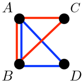
Figure 1: (color online). No-signaling monogamy diagram for two, tripartite Bell inequalities $\mathcal{B}_{ABC}$ (red) and $\mathcal{B}_{ABD}$ (blue). Only one of the inequalities can be violated by quantum theory.

Let us start with an example of tripartite Bell inequalities before we generalize our method to a more complex narrative.

The cornerstone of the method is a specific distance measure called statistical separation Kolmogorov50 ; Renyi70 ; DUTTA18 . This measure applies to $N$ probabilistic events but it is instructive to explain it first for $N=2$. We first define symmetric difference between two probabilistic events $A,B$ as $A\oplus B\equiv(A-B)\cup(B-A)$. A probability measure of the symmetric difference, $P(A\oplus B)$, is the statistical separation of the events $A$ and $B$. It can also be written as $P(A\oplus B)=P(A)+P(B)-2P(A\cap B)$. Note that the statistical separation conforms to all axioms of distance, including the triangle inequality: $P(A\oplus B)+P(B\oplus C)\geq P(A\oplus C)$. This is possible because in the symmetric difference every event is its own inverse, i.e., $A\oplus A=\varnothing$. The statistical separation can be extended to $N$ events inductively and we will briefly show it for $N=3$, sending the reader for more details to Ref. DUTTA18 .

In analogy to the two event symmetric difference, we define the three event one as $A\oplus B\oplus C\equiv(A\cap B\cap C)\cup(A\cap B^{c}\cap C^{c})\cup(A^{c}\cap B\cap C^{c})\cup(A^{c}\cap B^{c}\cap C)$. All three events in the brackets are mutually exclusive so the statistical separation reads $P(A\oplus B\oplus C)=P(A\cap B\cap C)+P(A\cap B^{c}\cap C^{c})+P(A^{c}\cap B\cap C^{c})+P(A^{c}\cap B^{c}\cap C)$. In the rest of the paper, for brevity, we write: $P(A_{i}\oplus B_{j}\oplus C_{k})=A_{i}B_{j}C_{k}$ with obvious generalizations for any $N$.

Consider now four parties $A,B,C$ and $D$. Each party has two choices of measurement settings indexed by a subscript $i$. For example, an event $A_{i}$ happens when the party $A$ sets the measurement $i$ and obtains an outcome $a_{i}$. First we consider binary outcomes $a_{i}$ for each setting $i$. Using the following triangle inequalities for the statistical separation

$$A_{1}B_{2}X_{2}+A_{2}B_{1}X_{2} \geq A_{1}B_{2}A_{2}B_{1},$$

$$A_{1}B_{2}A_{2}B_{1}+A_{2}B_{2}X_{1} \geq A_{1}B_{1}X_{1},$$ (1)

and adding them together, we arrive at the following Bell type inequality

$$\mathcal{B}_{ABX}=A_{1}B_{2}X_{2}+A_{2}B_{1}X_{2}+A_{2}B_{2}X_{1}-A_{1}B_{1}X_{1}\geq 0$$

(2)

where $X\in\{C,D\}$ (see Fig. 1). This separation Bell inequality is a generalization of the quadrangle inequality known in elementary geometry and first implemented to test local realism by Schumacher Schumacher91 . Recently, such Bell inequalities were derived and discussed for multipartite systems DUTTA18 . This inequality is violated by quantum mechanics with a GHZ state as shown in the Appendix C. The quantum mechanical violation is possible because in the derivation of the inequality (2) we assumed the existence of what we call the bridge separation $A_{1}B_{2}A_{2}B_{1}$, which is the statistical separation between the events corresponding to the measurements of non-commuting observables, $A_{1},A_{2}$ and $B_{1},B_{2}$ respectively. Obviously, in any local realistic (LR) model, the bridge separation exists but the quantum violation of (2) shows that it does not exist in quantum theory. This is along the lines of Fine’s paper Fine as the existence of the bridge separation would imply the existence of a joint probability distribution for non-commuting observables.

We now derive a monogamy relation for the violations of two Bell inequalities $\mathcal{B}_{ABC}$ and $\mathcal{B}_{ABD}$ in any no-signaling theory. Let us first note that every LR model trivially satisfies the monogamy inequality

$$\mathcal{B}_{ABC}+\mathcal{B}_{ABD}\geq 0.$$ (3)

This is becasue each term $\mathcal{B}_{ABC}$ and $\mathcal{B}_{ABD}$ is always non-negative for any LR model.

We now prove that the monogamy inequality (3) is obeyed by all no-signaling theories. It is a non-trivial observation because we know that there are no-signaling theories that can violate Bell inequalities. Quantum mechanics is an example of such a theory for which we can have $\mathcal{B}_{ABC}\leq 0$ and $\mathcal{B}_{ABD}\geq 0$ or the other way around. Thus, our claim is that for all no-signaling theories we have

$$\mathcal{M}_{AB}\equiv\mathcal{B}_{ABC}+\mathcal{B}_{ABD}\underset{\mathcal{NS}}{\geq}0.$$ (4)

$\mathcal{M}_{AB}$ is called the primary monogamy and it is the starting point for a slew of generalizations presented in this paper. The gist of our reasoning is to show that a suitable chaining of the triangle inequalities satisfied by any no-signaling theory leads to $\mathcal{B}_{ABC}$ and $\mathcal{B}_{ABD}$. We have

$$A_{1}B_{2}C_{2}+A_{1}B_{2}D_{2} \geq C_{2}D_{2},$$

$$C_{2}D_{2}+A_{2}B_{1}C_{2} \geq A_{2}B_{1}D_{2},$$

$$A_{2}B_{2}C_{1}+A_{2}B_{2}D_{1} \geq C_{1}D_{1},$$

$$C_{1}D_{1}+A_{1}B_{1}D_{1} \geq A_{1}B_{1}C_{1}.$$ (5)

Each triangle inequality has the bridge separation denoted by $C_{i}D_{i}$ with $i\in\{1,2\}$. The no-signaling principle guarantees that any given separation is independent on the context it was measured with: the separation $C_{2}D_{2}$ in the first triangle inequality is the same as the separation in the second triangle inequality. Without the no-signaling principle these two separations could be context dependent: $C_{2}D_{2}$ in the first inequality dependent on the context $A_{1}B_{2}$ and $C_{2}D_{2}$ in the second inequality dependent on the context $A_{2}B_{1}$. This fact makes each bridge separations $C_{i}D_{i}$ in (5) cancel out when all triangle inequalities are added, resulting in the monogamy relation (4)

$$A_{1}B_{2}C_{2}+A_{2}B_{1}C_{2}+A_{2}B_{2}C_{1}-A_{1}B_{1}C_{1}$$ (6)

$$+ A_{1}B_{2}D_{2}-A_{2}B_{1}D_{2}+A_{2}B_{2}D_{1}+A_{1}B_{1}D_{1}\underset{\mathcal{NS}}{\geq}0.$$

Note that the minus signs appear in two Bell functions $\mathcal{B}_{ABC}$ and $\mathcal{B}_{ABD}$ at certain positions that are a direct consequence of the separations’ geometric properties encoded in the inequalities (5). As we will see later, this simple observation has strong consequences that make our monogamies different and stronger from those reported in other papers Kurzynski11 ; Barrett06 ; Pawlowski09 ; Aolita12 . To be more precise, we could put the minus sign in the Bell function $B_{ABD}$ in front of any other separation without changing the monogamy and the physics of the problem. However, this innocent change leads to weaker no-signaling monogamies for more than two Bell functions as we will show below.

Example: 4 parties, 3-partite Bell inequalities.—To illustrate our approach, let us first do a warm-up with the simplest non-trivial scenario of four observers testing three-partite Bell inequalities.

Figure 2a depicts the geometry of three tripartite Bell inequalities: $\mathcal{B}_{ABC}$ (red), $\mathcal{B}_{ABD}$ (blue), and $\mathcal{B}_{ACD}$ (green). This geometry implies the following monogamy:

$$\mathcal{B}_{ABC}+\mathcal{B}_{ABD}+\mathcal{B}_{ACD}\underset{\mathcal{NS}}{\geq}0,$$ (7)

where each inequality reads

$$\mathcal{B}_{ABC} = A_{1}B_{2}C_{2}+A_{2}B_{1}C_{2}+A_{2}B_{2}C_{1}-A_{1}B_{1}C_{1},$$

$$\mathcal{B}_{ABD} = -A_{1}B_{2}D_{2}+A_{2}B_{1}D_{2}+A_{2}B_{2}D_{1}+A_{1}B_{1}D_{1},$$

$$\mathcal{B}_{ACD} = A_{1}C_{2}D_{2}-A_{2}C_{1}D_{2}+A_{2}C_{2}D_{1}+A_{1}C_{1}D_{1}.$$ (8)

The proof follows an observation that any pair of the Bell inequalities in (7) is the primary monogamy $\mathcal{M}_{AX}$ with $X=\{B,C,D\}$. Then, $\mathcal{M}_{AB},\mathcal{M}_{AC},\mathcal{M}_{AD}$ are greater or equal to zero and thus $\mathcal{M}_{AB}+\mathcal{M}_{AC}+\mathcal{M}_{AD}\geq 0$, which is exactly the formula (7). This new monogamy is strong in the sense that only one of the three Bell functions can be negative, leaving the other two compatible with LR.

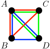
(a)

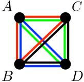
(b)

Figure 2: (color online). New monogamies for four tripartite Bell inequalities of $\mathcal{B}_{ABC}$ (red), $\mathcal{B}_{ABD}$ (blue), $\mathcal{B}_{ACD}$ (green), and $\mathcal{B}_{BCD}$ (black). (a) Strong monogamy states that only one of the inequalities $\mathcal{B}_{ABC},\mathcal{B}_{ABD}$, and $\mathcal{B}_{ACD}$ can be violated. (b) Full symmetric monogamy relation holds if we add one more Bell inequality $\mathcal{B}_{BCD}$.

Now we take a step further, throw in one more Bell inequality $\mathcal{B}_{BCD}$ (see Fig. 2b) and use the similar reasoning to prove that (see Appendix A)

$$\mathcal{B}_{ABC}+\mathcal{B}_{ABD}+\mathcal{B}_{ACD}+\mathcal{B}_{BCD}\underset{\mathcal{NS}}{\geq}0,$$ (9)

where the $\mathcal{B}_{BCD}$ is given by

$$\mathcal{B}_{BCD} = -B_{1}C_{2}D_{2}+B_{2}C_{1}D_{2}+B_{2}C_{2}D_{1}+B_{1}C_{1}D_{1}.$$

This is also a strong monogamy in the same way as before, i.e., only one Bell inequality can be violated by no-signaling correlations. In contrast, the Ref. Kurzynski11 derives a “Mermin monogamy” consisting of four Mermin inequalities such that three of them can be simultaneously violated by a four-qubit partially entangled state. Each inequality reads $E_{122}+E_{212}+E_{221}-E_{111}\leq 2$. Here, $E_{ijk}$ stands for the usual correlation function of the measurement results corresponding to the settings $ijk$. These correlation functions can be cast in the form of separation used in this paper, see for instance Ref. DUTTA18 . Note that all Mermin inequalities in their monogamy assign the minus sign to the correlation functions $E_{111}$. This leads to the simultaneous violations of up to three inequalities and thus to a weaker monogamy. This can be easily ‘fixed’ by changing the position of the minus sign in the inequalities—a fix that is not necessary in our method. Strong monogamies are definitely more desirable in quantum communication protocols such as cryptography, secret key sharing etc. Gisin02 ; Prabhu12 ; Giorgi11 ; Kumar16 . They also can be used in characterization of quantum many body systems as well as in quantum biology Chandran07 ; Song13 ; Qin16 ; Zhu12 ; Chanda14 .

Arbitrary number of parties.—We extend our monogamy relations for a general case of $N$ parties. For the binary outcomes, we introduce two sets of symmetric differences for $N$-party measurement events: $\mathcal{X}=\{A_{1}B_{2}\dots N_{2}$, and all cyclic permutations$\}$ and $\mathcal{Y}=\{A_{1}B_{1}\dots N_{1}\}$ for odd $N$, and for even $N$ one more term $A_{2}B_{2}\dots N_{2}$ is added to the set $\mathcal{X}$. In the set $\mathcal{X}$, each local measurement event with the setting $2$ appears an even number of times because of the cyclic permutations, so that these terms can be dropped out in deriving the $N$-party separation Bell inequalities. This is because every event in the symmetric difference is its own inverse, i.e., $X\oplus X=\varnothing$. Thus, the $N$-partite separation inequality reads $\mathcal{B}_{AB\dots N}=\sum_{i}P(\mathcal{X}_{i})-P(\mathcal{Y}_{1})\geq 0$, where the $\mathcal{X}_{i}$ implies the $i$th element of the set $\mathcal{X}$ and $\mathcal{Y}_{1}$ is the first element of the set $\mathcal{Y}$. Note that such a geometric inequality is invariant with respect to swapping of any one separation from the set $\mathcal{X}$ and the other from $\mathcal{Y}$. That is, all variants of Bell inequalities are equivalent. We show the quantum violations in the Appendix C.

With another party denoted by $N^{\prime}$ ($=N+1$), we have the following no-signaling primary monogamy: $\mathcal{B}_{A\dots N-1N}+\mathcal{B}_{A\dots N-1N^{\prime}}\geq 0$. Similar to the tripartite case, one can group the separations in the monogamy into two sets such that each of which has one separation with the minus sign. Then, as before, under the assumption of no-signaling, each set can be rewritten into two triangle inequalities linked via the context-independent bridge separations [see the argument below Eq. (5)]. Moreover, by using the primary monogamy we can derive the strong monogamy conditions for $N$-partite system: Any four $N$-partite Bell inequalities out of $(N+1)$ inequalities must hold the no-signaling monogamy relations. For $N=5$, one example of the strong monogamy is $\mathcal{B}_{ABCDE}+\mathcal{B}_{ABCDF}+\mathcal{B}_{ABCEF}+\mathcal{B}_{ABDEF}\geq 0$. The separations with minus sign for each inequality are $-A_{1}B_{1}C_{1}D_{1}E_{1},-A_{2}B_{2}C_{1}D_{2}F_{1},-A_{2}B_{2}C_{2}E_{1}F_{2}$, and $-A_{2}B_{2}D_{1}E_{2}F_{2}$. This is an example of an $AB$ division monogamy in the sense that the parties $A$ and $B$ are in the monogamous relations with the remaining parties. Note that because of the symmetries presented in our approach this holds for any two parties. For any $N$, our results can be extended to a $(N-3)$ division monogamy relations. A rule of assigning the minus sign to separations is as follows: for a given division, the minus is given to the separations in which the measurement settings for the remaining parties are $\{111,121,212,122\}$. Unlike the tripartite scenario, we cannot derive a fully symmetric monogamy relations for arbitrary $N$ where all Bell inequalities are involved. This is in contrast to the monogamy (9) and we conjecture that this can be improved if we consider the Bell inequalities with more separations or more than two measurement settings.

$d$-outcome scenario.—An extension for an arbitrary number of measurement outcomes $d$ requires a use of a quasi-distance—a metric that is not symmetric. Interestingly, our method still stands with a few simple modifications to account for the lack of symmetry.

We define a quasi-distance between events $A,B,C$ as $P([A+B]<C)\equiv\sum_{a,b}\sum_{c>[a+b]}P(A^{a},B^{b},C^{c})$. Here $P(A^{a},B^{b},C^{c})$ is the probability of a joint event where three parties detect the outcomes $a,b$, and $c$, respectively, and $[x]$ reads ‘$x$ modulo $d$’. It is trivial to check that it obeys all axioms of a proper distance sans symmetry.

Consider a tripartite scenario involving two choices of measurement settings $X_{i}$ $(i=1,2)$ each of which has $d$ possible outcomes: $X_{i}=0,1,\dots,d-1$. Using the properties of the quasi-distance (see Appendix B) we arrive at the following Bell inequality

$$\mathcal{B}_{ABC} = P([A_{1}+B_{2}]<C_{2})+P(C_{2}<[A_{2}+B_{1}])+P([A_{2}+B_{1}]<C_{1})-P([A_{1}+B_{2}]<C_{1})$$ (10)

$$+ P([A_{1}+B_{1}]<C_{2})+P(C_{2}<[A_{2}+B_{2}])+P([A_{2}+B_{2}]<C_{1})-P([A_{1}+B_{1}]<C_{1})\geq 0.$$

To get this inequality we followed exactly the steps outlined in the derivation of (1). Nothing has changed because those steps do not rely on the symmetry of the bridge separation.

We highlight that the Bell inequality (10) is the Svetlichny-type extension of the Zohren-Gill inequality Zohren08 ; Chen11 ; Bancal11 . By a simple swap $``[A+B]<C"\rightarrow``[A+B]>C"$ we get yet another Bell inequality. This inequality is violated by the generalized GHZ state (see Appendix C for more details).

By following exactly the same route as in the tripartite scenario discussed before (see Appendix B for more details) we arrive at the primary monogamy

$$\mathcal{B}_{ABC}+\mathcal{B}_{ABD}\underset{\mathcal{NS}}{\geq}0.$$ (11)

For an arbitrary $d$, the strong monogamy conditions for tripartite systems and their extension to multipartite cases are still unknown and they will be discussed elsewhere.

Conclusions.—Here we presented a new approach to a problem of monogamies for multipartite correlations with an arbitrary number of measurement outcomes. Our method is based on geometric properties of probability spaces called statistical separation, first introduced by Kolmogorov and developed further in the context of non-classical correlations in Renyi70 ; DUTTA18 ; Kolmogorov50 . The cornerstone of all results obtained in this paper is the triangle inequality for the statistical separation.

We derived new monogamies for $N$ parties, each performing measurement of two dichotomic observables. These monogamies are stronger than any other monogamies of this kind reported in the literature. They are stronger because of their strictly exclusivity, i.e., only one out of $N$ Bell inequalities can be violated. This can have potential applications in various quantum information protocols. It also improves our understanding of the relation between multipartite quantum, super-quantum correlations and no-signaling principle.

Using the similar geometric approach we also derived a new tripartite Svetlichny-Zohren-Gill type Bell inequality for two $d$-outcome measurements and showed its quantum violation. We also showed a no-signaling monogamy for this inequality. Interestingly, we had to use the quasi-distance in these derivations. As far as we know, this is the first usage of quasi-distance in the context of non-classical correlations. It would be interesting to see how to extend this to multipartite correlations and how to derive strong multipartite monogamies. This will be presented in a forthcoming work.

I acknowledgments

This research was supported by the National Research Foundation, Prime Minister’s Office, Singapore and the Ministry of Education, Singapore under the Research Centres of Excellence programme and Singapore Ministry of Education Academic Research Fund Tier 3 (Grant No. MOE2012-T3-1-009). J.L. acknowledges the financial support of the MSIT(Ministry of Science and ICT), Korea, under the ITRC(Information Technology Research Center) support program(IITP-2018-2015-0-00385) supervised by the IITP(Institute for Information & communications Technology Promotion) and the grant (No. 2014R1A2A1A10050117), funded by National Research Foundation of Korea (NRF) and the Korean government (MSIP).

Appendix A Primary monogamies

We show that any pair of Bell functions $\mathcal{B}_{ABC}$, $\mathcal{B}_{ABD}$, $\mathcal{B}_{ACD}$, and $\mathcal{B}_{BCD}$ obeys the primary monogamy and thus they hold the fully symmetric monogamy (9). It is enough to demonstrate a few cases because the proof is similar for any other pair.

For the Bell functions $\mathcal{B}_{ABC}$ and $\mathcal{B}_{ACD}$, the triangle inequalities read

$$A_{1}B_{2}C_{2}+A_{1}C_{2}D_{2} \geq B_{2}D_{2},$$

$$B_{2}D_{2}+A_{2}B_{2}C_{1} \geq A_{2}C_{1}D_{2},$$

$$A_{2}B_{1}C_{2}+A_{2}C_{2}D_{1} \geq B_{1}D_{1},$$

$$B_{1}D_{1}+A_{1}C_{1}D_{1} \geq A_{1}B_{1}C_{1}.$$ (12)

For the Bell functions $\mathcal{B}_{ABC}$ and $\mathcal{B}_{BCD}$,

$$A_{1}B_{2}C_{2}+B_{2}C_{2}D_{1} \geq A_{1}D_{1},$$

$$A_{1}D_{1}+B_{1}C_{1}D_{1} \geq A_{1}B_{1}C_{1},$$

$$A_{2}B_{2}C_{1}+B_{2}C_{1}D_{2} \geq A_{2}D_{2},$$

$$A_{2}D_{2}+A_{2}B_{1}C_{2} \geq B_{1}C_{2}D_{2}.$$ (13)

After adding them together some terms cancel leaving us with

$$\mathcal{B}_{ABC}+\mathcal{B}_{ABD}+\mathcal{B}_{ACD}+\mathcal{B}_{BCD}\geq 0.$$ (14)

Appendix B Quasi-distance

Here we provide details about the quasi-distance that were skipped in the main text. It is easy to verify that our quasi-distance is positive but not symmetric. Therefore, we need to prove that it obeys the triangle inequality. First, we show it for two events, i.e.,

$$P(A>B)+P(B>C)\geq P(A>C).$$ (15)

Here $P(X>Y)\equiv\sum_{x}\sum_{y<x}P(X^{x},Y^{y})$. A joint probability $P(X^{x},Y^{y})$ describes that two parties obtain the outcomes $x$ and $y$, respectively. To prove this, define the event $A\leq B\equiv\bigcup_{a\leq b}A^{a}\cap B^{b}$. It is trivial to see that $(A\leq B)\cap(B\leq C)\subseteq(A\leq C)$ and $(A>B)\cup(B>C)\supseteq(A>C)$, which implies the triangle inequality in (15). It is clear that the event $X>Y$ is not symmetric so the order of events in the triangle inequality is crucial.

For three events $A,B$, and $C$, we have $P([A+B]<C)\equiv\sum_{a,b}\sum_{c>[a+b]}P(A^{a},B^{b},C^{c})$. It is straightforward to show the following triangle inequality: $P([A+B]<C)+P(C<[D+E])\geq P([A+B]<[D+E])$. If we keep track of the order of events and chain the triangle inequalities, we get the Bell inequality (10) presented in the main text. The triangle inequalities read

$$P([A_{1}+B_{2}]<C_{2})+P(C_{2}<[A_{2}+B_{1}]) \geq P([A_{1}+B_{2}]<[A_{2}+B_{1}]),$$

$$P([A_{1}+B_{2}]<[A_{2}+B_{1}])+P([A_{2}+B_{1}]<C_{1}) \geq P([A_{1}+B_{2}]<C_{1}),$$

$$P([A_{1}+B_{1}]<C_{2})+P(C_{2}<[A_{2}+B_{2}]) \geq P([A_{1}+B_{1}]<[A_{2}+B_{2}]),$$

$$P([A_{1}+B_{1}]<[A_{2}+B_{2}])+P([A_{2}+B_{2}]<C_{1}) \geq P([A_{1}+B_{1}]<C_{1}).$$ (16)

As explained in the main text, another Bell inequality $\mathcal{B}_{ABD}$ can be derived by the swaps of the type $C_{i}\rightarrow D_{i}$ and $``<"\rightarrow``>"$. These swaps depend on the sign in the inequalities shown below and their logic is easier to understand from the inequalities in (17) rather than to describe in words. With this remark the following chain of triangle inequalities gives the monogamy $\mathcal{B}_{ABC}+\mathcal{B}_{ABD}\geq 0$:

$$P(D_{2}<[A_{1}+B_{2}])+P([A_{1}+B_{2}]<C_{2}) \geq P([D_{2}<C_{2}),$$

$$P([D_{2}<C_{2})+P(C_{2}<[A_{2}+B_{1}]) \geq P(D_{2}<[A_{2}+B_{1}]),$$

$$P(D_{1}<[A_{2}+B_{1}])+P([A_{2}+B_{1}]<C_{1}) \geq P([D_{1}<C_{1}),$$

$$P([D_{1}<C_{1})+P([A_{1}+B_{2}]<D_{1}) \geq P([A_{1}+B_{2}]<C_{1}),$$

$$P(D_{2}<[A_{1}+B_{1}])+P([A_{1}+B_{1}]<C_{2}) \geq P([D_{2}<C_{2}),$$

$$P([D_{2}<C_{2})+P(C_{2}<[A_{2}+B_{2}]) \geq P(D_{2}<[A_{2}+B_{2}]),$$

$$P(D_{1}<[A_{2}+B_{2}])+P([A_{2}+B_{2}]<C_{1}) \geq P([D_{1}<C_{1}),$$

$$P([D_{1}<C_{1})+P([A_{1}+B_{1}]<D_{1}) \geq P([A_{1}+B_{1}]<C_{1}).$$ (17)

Appendix C Quantum violations

We show the quantum violations of the Bell inequalities presented in the main text. The violations can be observed for the $N$-qudit GHZ state

$$|{\Psi}\rangle=\frac{1}{\sqrt{d}}\sum_{n=0}^{d-1}|{n}\rangle^{\otimes N}.$$ (18)

Each of the inequalities has two measurements per each observer.

Consider first the Bell inequality in terms of separations (binary outcomes). For odd $N$, it reads

$$P(A_{1}\oplus B_{2}\oplus\cdots\oplus N_{2})+\mbox{its cyclic permutations}$$ (19)

$$- P(A_{1}\oplus B_{1}\oplus\cdots\oplus N_{1})\geq 0.$$

For even $N$, one more separation $P(A_{2}\oplus B_{2}\oplus\cdots\oplus N_{2})$ is added, with a positive sign, to the inequality. Then, for the $N$-qubit GHZ state, i.e., $d=2$ in (18), the separation reads

$$P(A\oplus B\oplus\cdots\oplus N)=\frac{1}{2}\left(1+\left<\bigotimes_{s=1}^{N}\vec{b}_{s}\cdot\vec{\sigma}\right>\right),$$ (20)

where $\vec{b}_{s}$ are Bloch vectors of the local projectors for the observer $s$. Place $\vec{b}_{s}$ on the $x$-$y$ plane with $b_{sz}=0$. Introduce complex variables $b_{s}=b_{sx}+ib_{sy}$, where $b_{sx}$ and $b_{sy}$ are $x$ and $y$ components of the local Bloch vectors $\vec{b}$, respectively. Then,

$$\left<\bigotimes_{s=1}^{N}\vec{b}_{s}\cdot\vec{\sigma}\right>=\mathfrak{R}\left(\prod_{s}b_{s}\right),$$ (21)

where $\mathfrak{R}(b)$ is the real value of $b$. It is clear that the right-hand side removes imaginary terms, containing the even number of $b_{y}$’s. Letting $b_{sx}=\cos\theta_{s}$ and $b_{sy}=\sin\theta_{s}$, the complex variable $b_{s}=\exp(i\theta_{s})$ so that

$$\mathfrak{R}\left(\prod_{s}b_{s}\right)=\cos\theta,$$ (22)

where $\theta=\sum_{s}\theta_{s}$. Then, the separation reads

$$P(A\oplus B\oplus\cdots\oplus N) = \frac{1}{2}(1+\cos\theta)$$ (23)

$$= \begin{cases}1,&\mbox{if }\theta=2m\pi\\ 0,&\mbox{if }\theta=(2m+1)\pi\end{cases}$$

for an integer $m$. This is the perfect correlation for the GHZ state. Therefore, when we set the measurement setting $1$ as $x$ and the setting $2$ as $x$ rotated around $z$ by $\pi/(N-1)$ for each respective party, we will have that $-1\geq 0$ in (19) for odd $N$. For an even $N$, the Bell inequality includes one more term, $P(A_{2}\oplus B_{2}\oplus\cdots\oplus N_{2})=[1+\cos(\pi/(N-1))]/2$, not perfectly correlated. But we observe a violation (a weaker one) because all the other terms are still perfectly correlated.

For higher dimensional cases, we used the quasi-distance to derive Bell inequalities with two local measurements. To see the quantum violations, we use a Fourier basis

$$|{x}\rangle_{X_{i}} = \frac{1}{\sqrt{d}}\sum_{n=0}^{d-1}\omega^{n(x+\varphi_{i})}|{n}\rangle,$$ (24)

where $\omega=\exp(2\pi i/d)$ and $\varphi_{i}$ is a local phase of the $X_{i}$th measurement. Then, the probability $P(A^{a}_{i},B^{b}_{j},C^{c}_{k})$ to get the outcomes $a,b,c$ given the settings $i,j,k$ for a GHZ state (18) reads

$$P(A^{a}_{i},B^{b}_{j},C^{c}_{k})=\frac{1}{d^{4}}\left|\sum_{n=0}^{d-1}\omega^{n(a_{i}+b_{j}-c_{k}+\varphi_{ijk})}\right|^{2},$$ (25)

where $\varphi_{ijk}=\varphi_{i}+\varphi_{j}-\varphi_{k}$. To violate the Bell inequality, we set $\varphi_{121}=\varphi_{111}=1$, $\varphi_{122}=\varphi_{211}=\varphi_{112}=\varphi_{221}=1/3$, and $\varphi_{212}=\varphi_{222}=-1/3$. Figure 3 shows the quantum predictions of the left-hand side in (10) up to $d=50$. Negative values imply the violations.

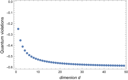
Figure 3: Value of the left-hand side of the Bell inequality in (10) as a function of the dimension $d$ up to $50$. As the lowerbound of the inequality by the local realistic description is zero, thus the negative values of the results imply the quantum violations.

References

- (1) J. S. Bell, Physics 1, 195 (1964).
- (2) J. F. Clauser, M. A. Horne, A. Shimony and R. A. Holt, Phys. Rev. Lett. 23, 880 (1969).
- (3) N. Brunner, D. Cavalcanti, S. Pironio, V. Scarani, and S. Wehner, Rev. Mod. Phys. 86, 419 (2014).
- (4) N. Bohr, Über die Serienspektra der Element. Zeitschrift für Physik, 2, 423–478 (1920).
- (5) D. M. Greenberger and M. A. Horne and A. Zeilinger, in Bell’s Theorem, Quantum Theory, and Conceptions of the Universe, edited by M. Kafatos (Kluwer, Dordrecht, 1989).
- (6) N. D. Mermin, Phys. Rev. Lett. 65, 1838 (1990).
- (7) J.-W. Pan, Z.-B. Chen, C.-Y. Lu, H. Weinfurter, A. Zeilinger, and M. Żukowski, Rev. Mod. Phys. 84, 777 (2012).
- (8) Ll. Masanes, A. Acín, and N. Gisin, Phys. Rev. A 73, 012112 (2006).
- (9) B. F. Toner, Proc. R. Soc. A 465, 59 (2009).
- (10) M. Pawłowski and Č. Brukner, Phys. Rev. Lett. 102, 030403 (2009).
- (11) L. Aolita, R. Gallego, A. Cabello, and A. Acín, Phys. Rev. Lett. 108, 100401 (2012).
- (12) R. Augusiak, M. Demianowicz, M. Pawłowski, J. Tura, and A. Acín, Phys. Rev. A 90, 052323 (2014).
- (13) R. Augusiak, Phys. Rev. A 95, 012113 (2017).
- (14) R. Horodecki, P. Horodecki, M. Horodecki, and K. Horodecki, Rev. Mod. Phys. 81, 865 (2009).
- (15) P. Kurzyński, T. Parerek, R. Ramanathan, W. Laskowski and D. Kaszlikowski, Phys. Rev. Lett. 106, 180402 (2011).
- (16) B. W. Schumacher, Phys. Rev. A 44, 7047 (1991).
- (17) P. Kurzyńsky and D. Kaszlikowski, Phys. Rev. A 89, 012103 (2014).
- (18) A. Kolmogorov, VI Zjazd Matematyków Polskich: Warszawa 20-23.IX.1948, Dodatek do Rocznika Polskiego Towarzystwa Matematycznego (Instytut Matematyczny Uniwersytetu Jagiellońskiego, 1950).
- (19) A. Renyi, Probability theory (North-Holland, Amsterdam, 1970).
- (20) A. Dutta, T.-U. Nahm, J. Lee, and M. Żukowski, New J. Phys. 20. 093006 (2018).
- (21) A. Fine, Phys. Rev. Lett. 48, 291 (1982).
- (22) J. Barrett, A. Kent, and S. Pironio, Phys. Rev. Lett. 97, 170409 (2006).
- (23) N. Gisin, G. Ribordy, W. Tittel, H. Zbinden, Rev. Mod. Phys. 74, 145 (2002).
- (24) R. Prabhu, A. K. Pati, A. Sen(De), U. Sen, Phys. Rev. A 85, 040102(R) (2012).
- (25) G. L. Giorgi, Phys. Rev. A 84, 054301 (2011).
- (26) A. Kumar, S. Singha Roy, A. K. Pal, R. Prabhu, A. Sen(De), U. Sen, Phys. Lett. A 380, 3588 (2016).
- (27) A. Chandran, D. Kaszlikowski, A. Sen(De), U. Sen,V. Vedral, Phys. Rev. Lett. 99, 170502 (2007).
- (28) X.-K. Song, T. Wu, L. Ye, Quantum Inf. Process. 12, 3305 (2013).
- (29) M. Qin, Z.-Z. Ren, X. Zhang, Quantum Inf. Process. 15, 255 (2016).
- (30) J. Zhu, S. Kais, A. Aspuru-Guzik, S. Rodriques, B. Brock, P. J. Love, J. Chem. Phys. 137, 074112 (2012).
- (31) T. Chanda, U. Mishra, A. Sen(De), U. Sen, arXiv:1412.6519 (2014).
- (32) S. Zohren and R. D. Gill, Phys. Rev. Lett. 100, 120406 (2008).
- (33) J.-L. Chen, D.-L. Deng, H.-Y. Su, C. Wu, and C. H. Oh, Phys. Rev. A 83, 022316 (2011).
- (34) J.-D. Bancal, N. Brunner, N. Gisin, and Y.-C. Liang, Phys. Rev. Lett. 106, 020405 (2011).