VLT/FLAMES high-resolution chemical abundances in Sculptor:
a textbook dwarf spheroidal galaxy^,

We present detailed chemical abundances for 99 red-giant branch stars in the centre of the Sculptor dwarf spheroidal galaxy, which have been obtained from high-resolution VLT/FLAMES spectroscopy. The abundances of Li, Na, $\alpha$-elements (O, Mg, Si, Ca Ti), iron-peak elements (Sc, Cr, Fe, Co, Ni, Zn), and $r$- and $s$-process elements (Ba, La, Nd, Eu) were all derived using stellar atmosphere models and semi-automated analysis techniques. The iron abundances populate the whole metallicity distribution of the galaxy with the exception of the very low metallicity tail, $-2.3\leq$ [Fe/H] $\leq-0.9$. There is a marked decrease in [$\alpha$/Fe] over our sample, from the Galactic halo plateau value at low [Fe/H] and then, after a ‘knee’, a decrease to sub-solar [$\alpha$/Fe] at high [Fe/H]. This is consistent with products of core-collapse supernovae dominating at early times, followed by the onset of supernovae type Ia as early as $\sim$12 Gyr ago. The $s$-process products from low-mass AGB stars also participate in the chemical evolution of Sculptor on a timescale comparable to that of supernovae type Ia. However, the $r$-process is consistent with having no time delay relative to core-collapse supernovae, at least at the later stages of the chemical evolution in Sculptor. Using the simple and well-behaved chemical evolution of Sculptor, we further derive empirical constraints on the relative importance of massive stars and supernovae type Ia to the nucleosynthesis of individual iron-peak and $\alpha$-elements. The most important contribution of supernovae type Ia is to the iron-peak elements: Fe, Cr, and Mn. There is, however, also a modest but non-negligible contribution to both the heavier $\alpha$-elements: S, Ca and Ti, and some of the iron-peak elements: Sc and Co. We see only a very small or no contribution to O, Mg, Ni, and Zn from supernovae type Ia in Sculptor. The observed chemical abundances in Sculptor show no evidence of a significantly different initial mass function, compared to that of the Milky Way. With the exception of neutron-capture elements at low [Fe/H], the scatter around mean trends in Sculptor for $\text{[Fe/H]}>-2.3$ is extremely low, and compatible with observational errors. Combined with the small scatter in the age-elemental abundances relation, this calls for an efficient mixing of metals in the gas in the centre of Sculptor since $\sim$12 Gyr ago.

1 Introduction

Measuring the detailed abundances of a variety of chemical elements in individual stars in a galaxy is the most accurate way to trace the chemical evolution processes through time. The chemical abundance pattern of each star is the product of the enrichment caused by all the previous generations of stars (e.g. Tinsley 1979, 1981; Matteucci & Francois 1989; McWilliam 1997). In the Local Group we are in the unique position to be able to study a wide range of galaxies in extraordinary detail, star by star. The signatures of different physical processes allow us to disentangle the star formation and evolutionary properties of nearby galaxies back to the earliest times.

The Sculptor dwarf spheroidal (dSph) galaxy is a satellite of the Milky Way at a distance of $86\pm 5$ kpc (Pietrzyński et al. 2008), and at high Galactic latitude ($b=-83$ degrees), with a systemic velocity, $v_{hel}=110.6\pm 0.5$ km s^-1 (Queloz et al. 1995a; Battaglia et al. 2008a). This makes it a relatively straightforward target for detailed studies of its resolved stellar population, as it is close enough for its red-giant branch (RGB) stars to be targeted with high-resolution (HR) spectroscopy. There is little Galactic foreground contamination, most of which can be easily distinguished by velocity and a careful analysis of the spectra (e.g. Battaglia & Starkenburg 2012). In contrast to the smaller ultra-faint dwarf (UFD) galaxies, the number of bright RGB stars that can be studied individually in a dSph is significantly larger, making the conclusions based on the properties of the resolved stellar population less prone to the effects of small number statistics.

There have been numerous photometric studies of the resolved stellar population in Sculptor since its discovery by Shapley in the 1930s, e.g. Hodge (1965); Norris & Bessell (1978); Kaluzny et al. (1995); Monkiewicz et al. (1999); Hurley-Keller et al. (1999); Majewski et al. (1999); Harbeck et al. (2001); Dolphin (2002); Maccarone et al. (2005); Babusiaux et al. (2005a); Westfall et al. (2006); Mapelli et al. (2009); Menzies et al. (2011); de Boer et al. (2011, 2012); Salaris et al. (2013); Martínez-Vázquez et al. (2015, 2016); Savino et al. (2018). This includes colour-magnitude diagram (CMD) analyses, but also the study of individual populations, such as the horizontal branch, X-ray binaries, blue stragglers and asymptotic giant branch (AGB) stars. The star formation history, coming from a careful CMD analysis, shows a peak in star formation $\sim$12 Gyr ago, with a subsequent tail-off in the star formation rate (de Boer et al. 2012), until Sculptor stopped forming stars $\sim$8 Gyr ago (e.g. Hurley-Keller et al. 1999; Dolphin 2002; de Boer et al. 2012). At the present time, Sculptor does not have any associated H I gas (Grcevich & Putman 2009). By combining CMD analysis with the spectroscopically determined metallicities for individual stars, de Boer et al. (2012) determined ages for the RGB stars in Sculptor. This made it possible for the first time to put accurate timescales on the chemical evolution processes in a dSph galaxy.

Early kinematic studies established that the Sculptor dSph is dominated by dark matter (Da Costa et al. 1991; Queloz et al. 1995b; Aaronson & Olszewski 1987; Tolstoy et al. 2001). The total mass of Sculptor is $(3.4\pm 0.7)\times 10^{8}$M_⊙, which represents a mass-to-light ratio of $158\pm 33\leavevmode\nobreak\$(M/L)_⊙ inside 1.8 kpc, with tentative evidence for a velocity gradient of $7.6^{+3.0}_{-2.2}$ km s${}^{-1}\,$deg^-1 (Battaglia et al. 2008a). This gradient can be interpreted as rotation about the minor axis, or it could be due to tidal disruption by the Milky Way. The combination of Hubble Space Telescope (HST) and Gaia observations of individual stars in Sculptor (Massari et al. 2018) has provided a new and accurate proper motion and orbit determination for Sculptor, which was further refined by Gaia DR2 results (Gaia Collaboration et al. 2018), see Table 1. These new determinations are fairly different from previous estimates in the literature (Schweitzer et al. 1995; Piatek et al. 2006; Walker et al. 2008; Sohn et al. 2017). In this relatively small and simple galaxy there are two distinct stellar populations present. They have different kinematics, metallicity, and spatial distributions (Tolstoy et al. 2004; Helmi et al. 2006; Coleman et al. 2005; Clementini et al. 2005; Battaglia et al. 2008a), with one population that is centrally concentrated, kinematically cold and relatively metal-rich; and another that is a more spatially extended, kinematically warmer, and more metal-poor.

Table 1: Astrometry of the Sculptor dwarf spheroidal galaxy by the Gaia Collaboration et al. (2018): the position on the sky ($\alpha$,$\delta$), parallax $\varpi$, proper motions ($\mu_{\alpha^{*}}$,$\mu_{\delta}$), and the elements of the covariance matrix, $\epsilon_{X}$. Also included are the number of member stars, $N_{\star}$ as determined by Gaia for the magnitude limit, $G_{\textsl{lim}}$.

The Sculptor dSph
$\alpha$	15.0392	deg
$\delta$	$-33.7092$	deg
$\varpi$	$-0.013$	mas
$\epsilon_{\varpi}$	0.004	mas
$\mu_{\alpha^{*}}$	0.082	mas/yr
$\epsilon_{\mu_{\alpha^{*}}}$	0.005	mas/yr
$\mu_{\delta}$	-0.131	mas/yr
$\epsilon_{\mu_{\delta}}$	0.004	mas/yr
$G_{lim}$	19.5	mag
$N_{\star}$	1592

The first detailed analysis of chemical abundances in Sculptor stars came from VLT/UVES spectra (Shetrone et al. 2003; Tolstoy et al. 2003; Geisler et al. 2005), examining 9 individual RGB stars in total. The position of the knee in the $\alpha$-elements was found to be at a significantly lower [Fe/H] than any other stellar system previously measured (Tolstoy et al. 2003; Venn et al. 2004). This sample of 9 stars, however, was too small to make concrete general conclusions, especially about the degree of scatter in the abundances. An extensive intermediate-resolution spectroscopic survey with Keck/Deimos of nearly 400 RGB stars around the centre of the Sculptor dSph determined the abundances of Fe, Mg, Ca, Si and Ti, using the synthesis of a large numbers of weak lines over a large wavelength range (Kirby et al. 2011). Other studies have focused on one or more individual stars (e.g. Smith & Dopita 1983; Shetrone et al. 1998; Salgado et al. 2016; Skúladóttir et al. 2015b), or individual elements, such as Mn (North et al. 2012). Recently, S and Zn were also measured in Sculptor (Skúladóttir et al. 2015b; Skúladóttir et al. 2017), and then compared directly to chemical abundances observed in damped Lyman-$\alpha$ systems observed at high redshifts (Skúladóttir et al. 2018).

Sculptor has also been the target of extensive searches for extremely metal-poor stars (Kirby et al. 2011; Starkenburg et al. 2010; Chiti et al. 2018), feeding high-resolution follow-ups to verify the detailed chemical abundances of this elusive population (Tafelmeyer et al. 2010; Frebel et al. 2010; Starkenburg et al. 2013; Jablonka et al. 2015; Simon et al. 2015; Chiti et al. 2018). Among these, the most metal-poor star outside the Milky Way was found at $\text{[Fe/H]}=-3.96\pm 0.06$ (Tafelmeyer et al. 2010). The metal-poor tail of the Sculptor dSph shows both similarities and differences with their counterparts in the Galactic halo.

In particular, the Milky Way halo stars show a bimodality in carbon (e.g. Aoki et al. 2007; Placco et al. 2014 and references therein), with two separated populations, above $\text{[C/Fe]}=0.7$ (CEMP stars), and below (C-normal stars). Among these, CEMP-no stars (with no enhancement in neutron-capture elements Ba or Eu abundances) are believed to show chemical signatures of the very first stars (e.g. Umeda & Nomoto 2002; Meynet et al. 2006). Carbon has been measured in sizeable samples of RGB stars in the Sculptor dSph using low-resolution (LR) spectroscopy: with Keck/Deimos by Kirby et al. (2015); VLT/VIMOS by Lardo et al. (2016), also including nitrogen; and with Magellan-Clay/M2FS by Chiti et al. (2018). Neither the HR surveys of extremely metal-poor stars (Tafelmeyer et al. 2010; Frebel et al. 2010; Starkenburg et al. 2013; Jablonka et al. 2015; Simon et al. 2015), nor the earlier LR studies (Kirby et al. 2015; Lardo et al. 2016) found any CEMP-no stars in Sculptor. However, one CEMP-no star was found at a surprisingly high $\text{[Fe/H]}=-2$ (Skúladóttir et al. 2015a), showing clear differences in [C/Fe] compared to other stars at this metallicity in Sculptor.

The recent study of Chiti et al. (2018), focusing on the most metal-poor tail in Sculptor ($\text{[Fe/H]}\leq-3$) with LR spectroscopy ($R\sim 2000$), found a trend of increasing [C/Fe] towards the lowest metallicities, as predicted in Salvadori et al. (2015). Their measured fraction of CEMP-no stars was 24% at $\text{[Fe/H]}\leq-3$, which is consistent with that observed in the Milky Way halo, $\sim$43% (Placco et al. 2014), given their errors. However, no CEMP-no stars were measured to have $\text{[C/Fe]}>+1$ in Sculptor, while the fraction of such stars in the Milky Way halo is $\sim$32% at $\text{[Fe/H]}\leq-3$ (Placco et al. 2014).

Table 2: Observing log, as well as the grating setting used for each spectrograph, the plate or fibre set used, the exposure time (Expt), the airmass (AirM) and when available the seeing measurement from the seeing monitor (DIMM).

Date	Setting	Plate	Expt (s)	AirM	DIMM
2003-08-24	HR10	MED1	3600	1.02	-
2003-08-24	HR10	MED1	3600	1.02	0.99
2003-08-28	HR10	MED2	3600	1.03	-
2003-08-25	HR10	MED2	5400	1.03	0.81
2003-08-22	HR13	MED1	3600	1.01	0.70
2003-08-22	HR13	MED1	3600	1.07	0.67
2003-08-20	HR13	MED2	4200	1.00	0.98
2003-08-20	HR13	MED2	4200	1.01	0.84
2003-08-21	HR14A	MED2	3600	1.01	0.66
2003-08-21	HR14A	MED2	3600	1.04	0.78
2003-08-21	HR14A	MED2	3600	1.14	0.66
2003-08-22	HR14A	MED2	4500	1.05	1.00
2003-08-21	HR14A	MED2	4700	1.04	0.84
2003-08-23	HR14A	MED2	5400	1.04	1.06
2003-08-23	HR15	MED1	3600	1.01	0.65
2003-08-23	HR15	MED1	3600	1.06	0.76
2003-08-23	580	FIB1	3600	1.01	0.65
2003-08-22	580	FIB1	3600	1.01	0.70
2003-08-23	580	FIB1	3600	1.06	0.76
2003-08-22	580	FIB1	3600	1.07	0.67
2003-08-20	580	FIB2	4200	1.00	0.00
2003-08-20	580	FIB2	4200	1.01	0.84
2003-08-24	580	FIB1	3600	1.02	-
2003-08-24	580	FIB1	3600	1.02	0.99
2003-08-28	580	FIB2	3600	1.03	-
2003-08-22	580	FIB2	4500	1.05	1.00
2003-08-21	580	FIB2	4700	1.04	0.84
2003-08-21	580	FIB2	5400	1.02	0.69
2003-08-25	580	FIB2	5400	1.03	0.81
2003-08-23	580	FIB2	5400	1.04	1.06
2003-08-21	580	FIB2	5400	1.14	0.66

Given the available large and detailed spectroscopic and photometric surveys of its stellar population, the Sculptor dSph is an obvious template for understanding galaxy formation and evolution on small scales. This galaxy has therefore also been the target of a large number of dedicated modelling efforts, using different techniques and approaches, e.g. Lanfranchi & Matteucci (2003, 2004); Fenner et al. (2006); Kawata et al. (2006); Salvadori et al. (2008); Marcolini et al. (2008); Revaz et al. (2009); Revaz & Jablonka (2012, 2018); Romano & Starkenburg (2013); Vincenzo et al. (2016); Côté et al. (2017).

Here we present HR spectra for 99 RGB stars in this galaxy taken with ESO VLT/FLAMES as part of the DART survey (Tolstoy et al. 2006). This study has been presented (without any technical details) in Tolstoy et al. (2009), and has already been used in a number of other publications. With the same spectra and stellar parameters as used here, North et al. (2012) measured Mn abundances in Sculptor and investigated its nucleosynthetic origin. The stellar parameters determined here have also been used in the study of S and Zn in this galaxy (Skúladóttir et al. 2015a; Skúladóttir et al. 2017). In addition, these results have been used in the verification of the Ca II triplet metallicity scale (Battaglia et al. 2008b; Starkenburg et al. 2010). The [Fe/H] and [$\alpha$/Fe] abundances were used in the CMD analysis in determining the star formation history in Sculptor (de Boer et al. 2012). The data presented here has also been used extensively as constraints for models, by Revaz et al. (2009); Revaz & Jablonka (2012, 2018); Romano & Starkenburg (2013); Côté et al. (2017).

Combining all the available results, it is clear that there are significant differences in the chemical abundances of Sculptor and the Milky Way, both at high and low metallicities. Detailed chemical abundances in Sculptor, such as those presented here, are therefore necessary to help us better understand this intriguing galaxy.

2 Data collection and pipeline processing

As part of the Paris Observatory VLT/FLAMES Guaranteed Time Observations (GTO) allocation, we carried out a spectroscopy programme of individual RGB stars over a 25$\arcmin$ diameter field of view at the centre of the Sculptor dSph galaxy. We simultaneously used FLAMES/GIRAFFE, in HR Medusa mode, and the fibre feed to the FLAMES/UVES spectrograph on VLT UT2 (Pasquini et al. 2002). These observations were carried out between 20-28 August 2003. In Table 2 the details of the observations are given.

2.1 Sample selection

Our target RGB stars were randomly selected within the FLAMES field of view from the I, (V-I) CMD shown in Fig. 1. The spatial scale of the targets are shown in Fig. 2. We limited ourselves to the upper part of the RGB, with I $<$ 17.5, to maximise the signal-to-noise (S/N). From the 132 fibres available in the Medusa mode of FLAMES/GIRAFE we allocated 117 to known and likely RGB stars in the Sculptor dSph, and 15 to monitor the sky background. For FLAMES/UVES, 6 fibres were allocated to RGB stars in Sculptor and 2 to the sky. The UVES configuration was changed once in the course of our FLAMES/GIRAFFE observations to give a total of 12 stars observed with FLAMES/UVES.

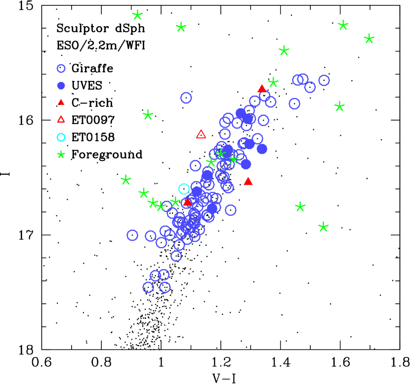
Figure 1: ESO/2.2m/WFI photometry (I, (V-I)) CMD of the central 30$\arcmin$ of Sculptor. Our spectroscopic target selection is overlaid. Foreground contamination stars are green asterisks and other symbols denote Sculptor members: blue circles for the main UVES (filled) and GIRAFFE (open) samples. The Li-rich star ET0158 is shown as a cyan open circle. Red filled triangles show C-rich stars and the CEMP-no star, ET0097, is shown as a red open triangle.

Table 3: Wavelength range, resolution and observing time of the GIRAFFE and UVES settings used here.

Setting	$\lambda_{\textit{min}}$	$\lambda_{\text{max}}$	Resolution	Obs. time
	[$\AA$]	[$\AA$]
HR10	5340	5620	19 800	4hr30min
HR13	6120	6400	22 500	4hr20min
HR14A	6390	6620	28 800	7hr
HR15	6610	6960	19 300	2hr
UVES	4800	6800	47 000	7 and 11hr

2.2 GIRAFFE and UVES fibre observations

For the FLAMES/GIRAFFE observations, one Medusa fibre configuration was used for four different wavelength regions (or settings), chosen to optimise the number Fe I and Fe II absorption lines and to observe specific $\alpha$-elements, iron-peak and heavy elements. The total observing time was $\sim$18 hours divided between 4 HR GIRAFFE settings: HR10, HR13, HR14A, and HR15, see Table 3. The resolution of these different settings ranges from $R\sim 19\,000-29\,000$.

The FLAMES/UVES fibres were fed into the red arm of UVES, centred at 580 nm, where the 1$\arcsec$ fibres yield a resolution $R\sim 47\,000$ over the wavelength range, see Table 3. Two FLAMES/UVES fibre configurations were used and one contained brighter targets than the other, and so the total exposure time spent on the six brighter and the six fainter targets amounted to 7 hr and 11 hr, respectively.

2.3 Pipeline reduction

The FLAMES/GIRAFFE spectra were reduced, extracted and wavelength calibrated using the GIRBLDRS pipeline provided by the FLAMES consortium (written by A. Blecha and G. Simon at Geneva Observatory). Each target spectrum was automatically continuum-corrected and cross-correlated with a spectral mask before being coadded. Various sky-subtraction schemes were tested, and there was a negligible difference between them for these HR spectra. We used the same sky-subtraction method as we have used on low-resolution Ca II triplet observations of Sculptor giants (Battaglia et al. 2008a) written by M. Irwin, which scales the sky background to be subtracted from each object spectrum to match the observed sky emission lines.

The radial velocities were measured by cross-correlating each of the four frames obtained with the HR10 setup spectra against a template (binary mask delivered within the GIRBLDRS pipeline). The measurements are reported in Table 7, showing the mean and the dispersion around the mean ($\rm 0.7\leavevmode\nobreak\ km\,s^{-1}$ on average) of these individual measurements. A further discussion about the radial velocities in this sample can be found in Skúladóttir et al. (2017), where systematic errors between observations taken from 2003-2013 were discussed in more detail. Six stars (ET0094, ET0139, ET0163, ET0173, ET0206, and ET0369) showed significant velocity variations, more than 2$\sigma$ from the median, and two stars (ET0097, and ET0109) showed moderate velocity variations, 1-2$\sigma$ from the median (Skúladóttir et al. 2017).

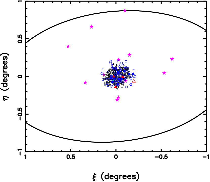
Figure 2: Spatial scale of Sculptor with tidal radius (black ellipse). Symbols are the same as in Fig. 1, with the addition of black open circles as LR data (Kirby et al. 2011) and magenta stars as HR data from the literature (Shetrone et al. 2003; Geisler et al. 2005; Frebel et al. 2010; Starkenburg et al. 2013; Simon et al. 2015; Jablonka et al. 2015).

For equivalent width (EW) determination, we used DAOspec (Stetson & Pancino 2008), which determines EWs from Gaussian fitting for a single FWHM value, determined per target, combined with an iterative fit to the global continuum (examined further by Letarte et al. 2010). We were able to verify the zero point accuracy of the FLAMES/GIRAFFE observations for both velocity and EW determinations by deliberately reobserving six stars previously observed with UVES and analysed by Shetrone et al. (2003) and Geisler et al. (2005). These UVES spectra have both a broader wavelength coverage and higher resolution than the newer GIRAFFE spectra. They thus provide a calibration of the automated methods used here as well as a comparison to the limited wavelength range of the GIRAFFE spectra.

The FLAMES/UVES fibre spectra were treated similarly to GIRAFFE spectra: they were reduced using the FLUVES pipeline (Modigliani et al. 2004), sky-subtracted using the same recipe as for GIRAFFE spectra albeit using a single sky fibre, and radial velocities were obtained by cross-correlating the individual 3 to 13 exposures for each star to a template (the observed spectrum, shifted to rest-frame, of star H497 from Shetrone et al. 2003). Table 7 reports the mean and dispersion around the mean of these measurements. For the EW determination from these higher resolution spectra, gaussian fits using a single full width half maximum (as performed by DAOspec) is not adequate for the stronger lines, so that EWs were measured manually with the standard splot routine in IRAF.

2.4 Pipeline output and member selection

From the radial velocities, $v_{r}$, we determined if each star is a likely member of the Sculptor dSph. We also checked the quality (S/N) of the spectra, and if the star is likely to be an RGB star. The S/N for the GIRAFFE spectra was estimated as the inverse of the residuals reported by DAOspec, averaged over all four setups (HR10, HR13, HR14A and HR15). This is only intended to give an indication of the relative quality of the spectra. The S/N reported for the UVES spectra was estimated in a more traditional way, by assessing the dispersion around the continuum in a line-free region of the spectrum around 6400 Å.

Stars that are not likely members of Sculptor, are not RGB stars, or have spectra of too low quality are removed from further analysis at this point. Table 7 lists the entire target list for our observations, including non-members and other stars we could not analyse properly. We include the available photometry, V, I, J, K filters (Babusiaux et al. 2005b; Battaglia et al. 2008b), and the measured radial velocities, v_r, from the HR10 grating (see previous section), the final coadded S/N of the spectra and also the cross-IDs of stars previously observed with UVES in slit mode.

From the 117 stars observed with GIRAFFE, 17 were found to be non-members based on their radial velocities. One additional star (ET0092) was rejected because its spectroscopic gravity showed it to be a foreground Galactic sub-giant, with a radial velocity comparable to that of Sculptor. This was also confirmed by an independent automatic classification (Kordopatis et al. 2013). Six stars were excluded because of low S/N, two of those had $\text{S/N}\leq 13$, and other four had low $\text{S/N}\leq 25$ combined with low metallicity, $\text{[Fe/H]}<-2$. One GIRAFFE spectrum (star ET0041) was severely affected by a CCD defect (a bad column) running right through the centre of the fibre image, and was therefore also discarded. One C-star (ET0167, star number 3 from Azzopardi et al. 1985) and 2 CN-rich stars (ET0136 and ET0315) were also rejected from further analysis, see Fig. 1, because of the severe blending created by the forest of CN molecular lines. This left 89 stars in the GIRAFFE sample that could be fully analysed. The 12 FLAMES/UVES target stars were all known to be Sculptor dSph members from previous observations. Two stars were found to have too low S/N for a reliable analysis, and were excluded, leaving a total of 10 UVES spectra. Thus, the full sample of FLAMES observations for which we could proceed to derive stellar parameters, metallicities and detailed abundance ratios consists of 99 stars (89 from the GIRAFFE and 10 from the UVES samples).

To further our membership analysis based on radial velocities and gravities, we also inspected the Gaia DR2 candidate members for Sculptor (Gaia Collaboration et al. 2018) which is based on proper motions and CMD position. All our proposed members are in this catalogue, with the exception of six stars (ET0024, ET0048, ET0109, ET0137, ET0173 and ET0378), which have proper motions compatible with Sculptor but were discarded from the Sculptor members because of their location in the Gaia DR2 (G,(BP-RP)) CMD. Conversely, one star in the Gaia Collaboration et al. (2018) catalogue is discarded as a Sculptor member in the present work based on its radial velocity (ET0124). We are thus confident that the members that we have identified here are indeed members of Sculptor.

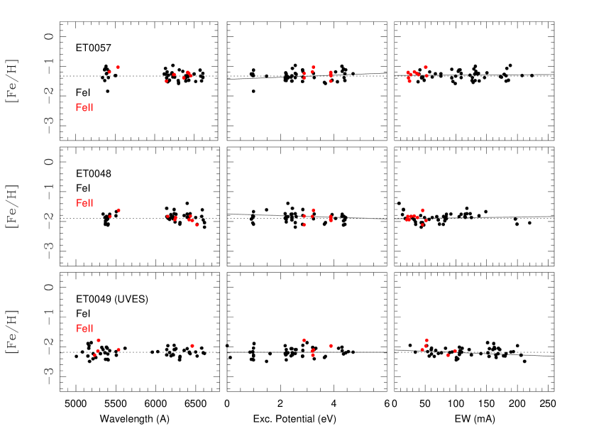
Figure 3: Diagnostic plots for three typical stars in our sample. Top row: ET0057, $\text{[Fe/H]}=-1.3$, GIRAFFE. Middle row: ET0048, $\text{[Fe/H]}=-1.9$, GIRAFFE. Bottom row: UET0049, $\text{[Fe/H]}=-2.2$, UVES. For each star, iron abundances (Fe I: black; Fe II: red) are plotted against wavelength, excitation potential and EW of the line. Dotted lines are the mean [Fe/H] of each star while solid lines show the slopes of best fits.

3 Stellar parameters and model atmospheres

A comprehensive model atmosphere abundance analysis was performed for our sample of 99 stars in Sculptor’s central field. The GIRAFFE and UVES spectra were treated separately, because of the difference in spectral resolution and wavelength range, see Table 3. We follow the method outlined in Shetrone et al. (2003) and Venn et al. (2012) for the UVES spectra, and that outlined by Letarte et al. (2010) and Lemasle et al. (2012, 2014) for the GIRAFFE spectra, with some minor adjustments to take advantage of the higher signal to noise ratio of the present sample.

3.1 The line list

The line list and atomic data (excitation potential, $\chi$, and log$\,gf$) were adopted from Shetrone et al. (2003), with a few additional lines selected from the work of Pompéia et al. (2008) in the LMC. The broadening coefficients (C6) were updated from Barklem et al. (2000); Barklem & Aspelund-Johansson (2005). All the lines were carefully examined using spectral synthesis to ensure there were no significant blends at our metallicity range in Sculptor, given the GIRAFFE spectral resolution. These were also compared to the previously published UVES results (Shetrone et al. 2003; Geisler et al. 2005) using the overlapping sample. The continuum level is more difficult to determine at the lower spectral resolution of the GIRAFFE spectra. In addition, it can be affected by CN molecular features. Thus, we have been careful to only adopt lines that are not contaminated by these features for the abundance analysis. The resulting list of reliable stellar absorption lines in our spectra, within the GIRAFFE wavelength range (and including additional lines which are used for the UVES spectra) is given in Table C.

3.2 Stellar parameters - photometry

The initial estimates for effective temperature, T_eff, and surface gravity, log g, are based on photometry. The V and I photometry come from the ESO-MPG 2.2 m telecope and the wide field imager, WFI (Battaglia et al. 2008b). The J and K_s photometry, available for a sub-sample of the observed stars, come from the Cambridge Infrared Survey Instrument (Babusiaux et al. 2005b). The T_eff of all observed stars were determined using the (V-I), and where possible also (V-J) and (V-K_s) temperature calibrations of Ramírez & Meléndez (2005), after global dereddening by E(B-V) $=$ 0.02, with A(V) $=$ E(B-V)$\times$3.24, E(V-I) $=$ E(B-V)$\times$1.28, E(V-K) $=$ E(B-V)$\times$2.87, E(V-J) $=$ E(B-V)$\times$2.335. Initial metallicity estimates used in the colour-temperature calibration were taken from the LR Ca II triplet survey (Battaglia et al. 2008a). The (V-I) and (V-K) colours and temperatures are listed in Table C, which also includes the physical surface gravity based on the bolometric correction from Alonso et al. (1999), assuming the photometric temperature and the initial metallicity for each star, to calculate M_bol. A distance modulus of (M-m)${}_{\rm o}=19.54$ was adopted from Mateo (1998), as in Tolstoy et al. (2003), and a mass of 0.8$\,M_{\sun}$ for each star is assumed to be a reasonable hypothesis, given the age range of the sample (see de Boer et al. 2012).

We found the temperatures determined from (V-I) to be on average 200 K hotter than those from (V-J) or (V-K_s) for the sub-sample of stars that had IR photometry (56 stars out of the total sample of 99). Since the cause of this offset is not clear, the (V-I), (V-J) and (V-K_s) temperature results were averaged together. In the case where either (V-I) or the IR colours were missing, an average offset was applied to ensure that all stars are on the same mean temperature scale.

One possibility to explain this inconsistency would be zero point uncertainties in the photometry. When we used the infrared based temperatures alone, (V-J) or (V-K_s), the stellar gravities deduced from ionisation equilibrium of Fe i and Fe ii, were too low by a large factor ($\Delta\text{log\leavevmode\nobreak\ g}=0.75$ dex) compared to photometric gravities. A simple zero-point shift in the I photometry to bring (V-I) temperatures in line with infrared ones would therefore result in a temperature scale producing a very uncomfortable ionisation balance. Conversely, shifting the infrared colours to the (V-I) temperature scale required an unreasonably large zero-point offset in the K and J-band photometry. The solution adopted here (averaging the temperature from three colour indices) produces a temperature scale in good agreement with excitation and ionisation equilibria of the iron lines, and was therefore preferred.

Figure 4: Global quality of the stellar parameters over the sample. The upper two panels display the distribution of the slopes for [Fe I/H] abundances with respect to the excitation potential $\chi_{ex}$ (left); and EWs of lines (right). The lower two panels show the distribution of the ionisation balance, $\rm[{Fe\textsc{I}}/H]-[{Fe\textsc{II}}/H]$, (left); and dispersion of Fe abundances from individual lines around the mean (right).

3.3 Stellar parameters - spectroscopy

Iron lines, Fe I and Fe II, were identified (see Table C), measured in all spectra, and used to constrain the stellar parameters. Model atmospheres are OSMARCS models kindly provided by Plez (private communication 2000-2002), computed with the MARCS code, initially developed by Gustafsson et al. (1975) and subsequently updated by Plez (1992), Edvardsson et al. (1993) and Asplund et al. (1997). In the metallicity range $\text{[Fe/H]}<-1$, this grid assumes a standard $\text{[$\alpha$/Fe]}=+0.4$, which overestimates the actual [$\alpha$/Fe] in Sculptor for stars with metallicities $\text{[Fe/H]}>-2$. The metallicities assumed in the models were therefore corrected to account for this effect, by lowering the actual iron abundance of the star by a factor ensuring that the overall metallicity of the star was conserved.

Abundance calculations were performed using CALRAI, an LTE spectrum synthesis code originally developed by Spite (1967), with numerous updates and improvements over the years. Abundances from individual lines are computed, and the measurement uncertainty on each EW ($\delta_{\rm DAO}$, estimated by DAOspec) is propagated into an uncertainty in the resulting abundance for each line. The error estimates on abundances are then carried throughout the stellar parameter and abundance derivation, by weighting each line by $1/(\delta_{\rm DAO})^{2}$ in the computations of slopes or means.

The curve of growth for Fe was examined for each star as a final check that both the Fe i and Fe ii lines are well fitted using the adopted parameters for all line strengths. Measurements of Fe as a function of $\lambda$, line excitation potential and EW for the adopted stellar parameters are shown for three typical stars in Fig. 3. An overview of the relevant tests for Fe measurments in GIRAFFE and UVES is shown in Fig. 4, which includes the distribution of the slopes for [Fe i/H] abundances with respect to the line excitation potential and EW; the distribution of residual [Fe i/H]-[Fe ii/H] (ionisation balance); and the distribution of observed dispersion of Fe abundances from individual lines around the mean ($\sigma_{\rm X}$). There is a slight shift in the distributions of $\sigma_{\rm{Fe\textsc{i}}}$ and $\sigma_{\rm{Fe\textsc{ii}}}$, arising from the fewer lines of Fe II measured.

3.3.1 Microturbulence velocities v_t

The microturbulence velocities, v_t, were determined by requiring a match between the Fe I abundances and their expected EWs. Using expected EWs rather than the observed strength of the line removes a bias towards higher v_t  which is created by the correlated errors between measured EWs and Fe abundances of individual lines, as first highlighted by Magain (1984) and more recently explored by Hill et al. (2011). This also allows more efficient identification of false detections of faint lines. The Fe abundance was then checked against that adopted for these initial calculations, then iterated until the model metallicity matched the final measured Fe i abundances. The uncertainty on v_t, for each star, was evaluated from the uncertainty in the slope of the Fe I abundances with line strength. The final v_t uncertainties are on average $\pm$0.20 km s^-1.

3.3.2 Effective temperatures T_eff

The initial photometric estimates of T_eff were checked by examining the relation between the Fe i line abundances and the excitation potential, $\chi$. The result was re-examined for any star with a slope $\geq 2\sigma$. This included 25 stars of the 89 GIRAFFE targets, and 1 of the UVES targets. In the majority of the cases, the slopes were found to be simply due to a large dispersion in the Fe i abundances. For 11 GIRAFFE and 1 UVES targets however, the initial temperature estimates (from photometry) were adjusted to provide an acceptable excitation equilibrium. These adjustments were in random directions, and all within 100 K of the initial temperature except in two cases, ET0330 which required a $-150$ K temperature decrease and ET0241 a $+200$ K temperature rise. The latter, ET0241, only had available temperature from one colour, (V-I), while ET0330 had also the IR photometry.

3.3.3 Surface gravities log g

The photometric estimates of log g were adjusted to ensure that the same abundance of iron is determined from the neutral and ionised Fe lines, within uncertainties. More precisely, we required that $|\rm[{Fe\textsc{I}}/H]-[{Fe\textsc{II}}/H]|\leq 2\times\rm\sqrt{(}\sigma_{\rm{Fe\textsc{I}}}^{2}+\sigma_{\rm{Fe\textsc{II}}}^{2})$. These spectroscopic log g values were adopted in the abundance analysis, and are listed in Table C. The uncertainty on log g was evaluated from the uncertainties on the Fe I and Fe II abundances, and is on average 0.31 dex. Our spectroscopic values have a lower limit, $\text{log\leavevmode\nobreak\ g}\geq 0.0$, due to the limits of the available grid of stellar atmosphere models. Only six stars actually hit this limit, and of those, only two have Fe out of ionisation equilibrium (see Table C).

4 Abundance determinations

The FLAMES/GIRAFFE spectra present some challenges because of the limited wavelength coverage and rather low spectral resolution (e.g. Pompéia et al. 2008; Letarte et al. 2010), compared to that used by classical HR abundance analysis. To ensure homogeneity, however, we have chosen to perform an analysis as similar as possible for our GIRAFFE and UVES spectra.

The abundances of the chemical elements were determined from EW measurements, which are listed in table 10. Hyperfine structure (HFS) corrections were included for: Ba II 6141 and 6496 Å (Rutten 1978, the isotopic solar composition from McWilliam 1998); La II 6320 Å (Lawler et al. 2001a, with the oscillator strength from Bord et al. 1996); and Eu II 6645 Å (Lawler et al. 2001b, using the oscillator strength from Shetrone et al. 2001). The HFS corrections are small or negligible for these lines, ranging from zero to 0.14 dex, with the strongest dependence on the line strength. HFS corrections were also computed for the Co I 5483 line (using atomic data from Prochaska et al. 2000), which proved to be larger (ranging from 0.03 to 1.0 dex) and primarily dependent on both line strength and v_t. HFS was not included for the Ba II line at 5854 Å  which was only available for the UVES spectra. The effects are expected to be small (e.g. Mashonkina & Zhao 2006), and in fact it agreed with the other lines, with no significant offset.

The most metal-poor stars in our sample ($\rm[Fe/H]\leq-2.2$) all happen to have been observed with GIRAFFE. The weak spectral lines coupled with the somewhat limited spectral resolution of the GIRAFFE spectra make these measurements less reliable. Thus, we have taken extra care to analyse these stars. We note that these stars have metallicities in agreement with the Ca II triplet results from our LR survey (Battaglia et al. 2008b). No corrections have been made to our abundances for non-LTE effects. We have attempted to compare our abundances with similar LTE analyses to minimise this source of error.

Table 4: Abundance errors arising from uncertainties in stellar parameters over our full sample. The average uncertainties of our stellar parameters: $\delta\text{T${}_{\rm eff}$}=\pm 100$ K, $\delta\text{log\leavevmode\nobreak\ g}=\pm 0.31$, $\delta\text{v${}_{\rm t}$}=\pm 0.20$

. [X/Y] $\Delta[X/Y]_{\text{T${}_{\rm eff}$,log\leavevmode\nobreak\ g}}$ $\Delta[X/Y]_{\text{vt}}$ $\sigma_{\rm mod}$ [Fe I/H] +0.13 $-0.08$ 0.16 [O I/Fe] +0.06 +0.02 0.06 [Na I/Fe] $-0.06$ +0.08 0.10 [Mg I/Fe] $-0.11$ $-0.01$ 0.11 [Al I/Fe] $-0.06$ +0.08 0.11 [SI I/Fe] $-0.10$ +0.08 0.13 [Ca I/Fe] $-0.03$ +0.02 0.05 [Sc II/Fe] $-0.02$ +0.07 0.08 [Ti I/Fe] +0.04 +0.06 0.08 [Ti II/Fe] $-0.04$ +0.02 0.06 [Cr I/Fe] +0.06 $-0.01$ 0.07 [Co I/Fe] +0.02 +0.02 0.05 [Ni I/Fe] $-0.02$ +0.02 0.08 [Zn I/Fe] $-0.12$ +0.03 0.13 [Ba II/Fe] +0.01 $-0.10$ 0.11 [La II/Fe] +0.02 +0.07 0.08 [Eu II/Fe] $-0.02$ +0.06 0.07

4.1 Error estimates

Uncertainties on individual elemental abundances were estimated from three different sources:

• Individual errors on EW measurements are given by DAOspec and are propagated through the abundance calculations to produce an individual error on each single line measurement ($\rm\delta_{DAOi}$ for each line $i$), and propagated on the mean abundance for each element X, $\rm\delta_{DAO}(X)$.

• The dispersion ($\rm\sigma_{obs}$) around the mean abundance of a given species measured from several lines reflects a combination of line measurement errors, uncertainties on atomic data and modelling errors.

• Abundance errors due to uncertainties in the stellar parameters of the targets were estimated by re-computing abundances with varying stellar parameters (T_eff, log g, v_t), according to the individual error estimates on the stellar parameters. Because of the strong covariance between T_eff and log g, astrophysically bound by stellar evolution, we varied T_eff and log g in lock-step while v_t was varied on its own. The overall error due to stellar parameter uncertainties ($\rm\sigma_{mod}$) is then computed as the quadratic sum of the uncertainties arising from (T_eff + log g) and v_t. Table 4 reports the mean over the sample of these errors.

The line measurement and atomic data uncertainties were combined into an observational error on the abundance of element X:

$$\rm err_{obs}(X)=max(\delta_{DAO}(X),\sigma_{obs}/\sqrt{N_{X}})$$

where $\rm N_{X}$ is the number of lines measured for element X and $\rm\sigma_{obs}$ is set to $\rm\sigma_{obs}(X)$ if $\rm N_{X}>3$ or to $\rm\sigma_{obs}(Fe)$ if $\rm N_{X}\leq 3$. That is, we use the dispersion of iron around the mean in each star as a surrogate for the dispersion around the mean abundance when too few lines of element X are available to robustly estimate this dispersion. This observational error $\rm err_{obs}(X)$ is then combined quadratically with the overall error due to stellar parameters $\rm\sigma_{mod}$ to estimate the final error on abundances, provided in Table 11.

4.2 Verification of the abundance analysis

Several tests were made to ensure that the abundance analysis of the FLAMES/GIRAFFE spectra was reliable. For this purpose, six stars with previously published analysis from UVES slit spectra (Shetrone et al. 2003; Geisler et al. 2005) were reobserved with GIRAFFE. In these tests we compared: stellar abundances; EW measurements; and elemental abundance results, between present and previous work. In addition, we made a comparison with the results for the carbon-enhanced metal-poor (CEMP-no) star ET0097, obtained with UVES slit spectroscopy (Skúladóttir et al. 2015b). This verification process showed the results of our GIRAFFE analysis to be reliable. For more details see Appendix A.

5 Results

Elemental abundances have been measured for 89 (82 new) stars in the Sculptor dSph from FLAMES/GIRAFFE and 10 new stars with FLAMES/UVES spectroscopy. We have focused our attention on seventeen elements to characterise the light elements (Li, Na), $\alpha$-elements (O, Mg, Si, Ca, Ti), iron-peak elements (Sc, Cr, Fe, Co, Ni, Zn), and heavy elements (Ba, La, Nd, Eu). The results of the abundance measurements are listed in Table 11.

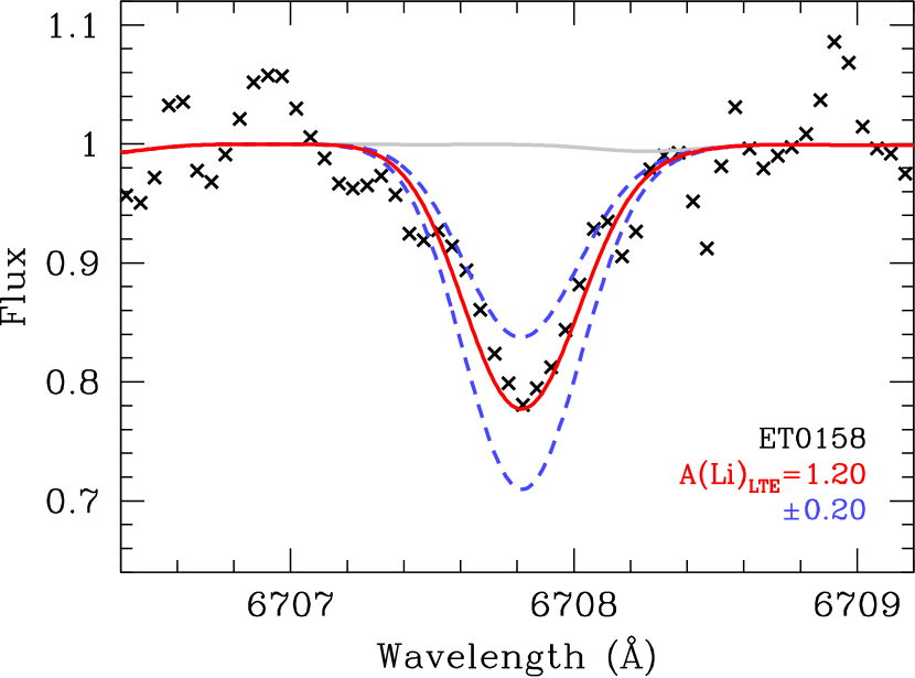
Figure 5: Spectra of the Li I line at 6707.8 Å in the star ET0158. Black crosses show our GIRAFFE spectrum, the red line is the best fit at $\text{A(Li)}_{\text{LTE}}=1.20$, and blue dashed lines show $\pm 0.2$ dex from this value. The grey solid line is the case with no Li present.

5.1 Li detection

As Li is destroyed in stellar interiors, Li-poor material is mixed up to the surface at later stages of stellar evolution (e.g. Gratton et al. 2000), and Li abundances in giant stars are typically very low. However, Li-enhanced giants have been found in moderate numbers in various environments (Monaco & Bonifacio 2008; Gonzalez et al. 2009; Monaco et al. 2011; Ruchti et al. 2011; Kirby et al. 2012, 2016; Martell & Shetrone 2013; Liu et al. 2014; Casey et al. 2016; Delgado Mena et al. 2016). Explaining the high Li in these stars requires either a mechanism to avoid depletion or an extra source of Li, apart from the amount the star was born with.

In our FLAMES/GIRAFFE+UVES sample of 99 giant stars in Sculptor, we could detect Li in only one star, ET0158, see Fig. 5, which has $\text{A(Li)}_{\text{LTE}}=1.20\pm 0.26$, and a metallicity of $\text{[Fe/H]}=-1.80\pm 0.21$. Applying NLTE-corrections provided by Lind et al. (2009a) results in $\text{A(Li)}_{\text{NLTE}}=1.40\pm 0.26$ for ET0158. The detection limit in our sample was $\leq 0.5$ dex in the mean, so for this sample of giant stars in Sculptor with $V\lesssim 18.4$ (or $M_{V}\lesssim-1.1.$), we estimate a fraction of $1\%^{+2.3}_{-0.8}$ (errors from Gehrels 1986) of the stars to have $\text{A(Li)}_{\text{LTE}}>0.5$.

5.1.1 Comparison with literature data

In a sample of $\approx$400 giant stars in the Milky Way bulge, Gonzalez et al. (2009) found 13 Li-detections ($\approx$3%). Two of these stars have very high values, $\text{A(Li)}_{\text{NLTE}}>2.5$, but for the other 11 stars a correlation between T_eff and Li abundance was found (also seen for different samples in Brown et al. 1989; Pilachowski et al. 1990, 2000; Lebzelter et al. 2012). Somewhat surprisingly, the Sculptor star ET0158, seems to fall directly onto this relation, see Fig. 6. Compared to the bulge sample, ET0158 has very different metallicity and luminosity, so this is not necessarily expected. With a sample of only one star it is quite possible, however, that ET0158 lands on this relation by mere chance. Also included in Fig. 6 are two Li-rich giants in Sculptor from Keck II DEIMOS medium-resolution spectroscopy (Kirby et al. 2012). The more Li-rich of these two clearly falls off the relation, in a similar way to the two Li-rich giants in the bulge sample, while the other one is more ambiguous.

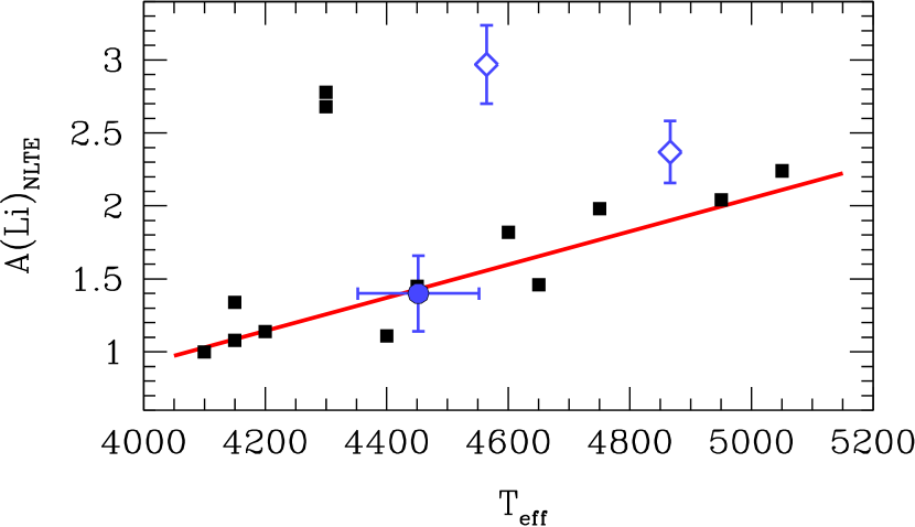
Figure 6: Lithium detections in Sculptor giants (blue) as a function of T_eff. The filled circle is ET0158, and open diamonds are two Li-rich giants from Kirby et al. (2012). The red line shows the trend found by Gonzalez et al. (2009) for Galactic bulge giants (black squares) with $1\leq\text{A(Li)}_{\text{NLTE}}\leq 2.5$.

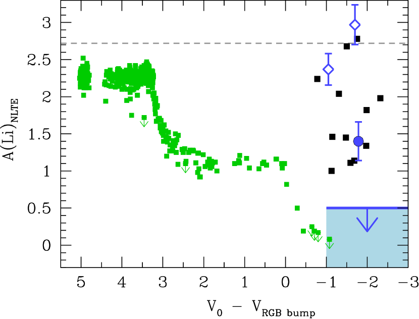
Figure 7: Lithium abundances as a function of ${V_{0}}$ relative to the predicted $V_{\text{RGB bump}}$ (Ferraro et al. 1999), for Sculptor and Milky Way bulge giants (same symbols as in Fig. 6). The typical detection limit of our FLAMES sample, $\text{A(Li)}_{\text{LTE}}=0.5$, is shown with a blue line, and upper limits for non-detections lie in the shaded region. The globular cluster NGC 6397 is also shown with small green squares (Lind et al. 2009b). The primordial Li abundance is shown with a grey dashed line (Coc et al. 2012).

Following the approach of Kirby et al. (2012), the Li-abundance is plotted in Fig. 7, as a function of the de-redenned magnitude of the star, relative to the RGB bump luminosity ($V_{\rm o}-V_{\text{RGB bump}}$). The predicted $V_{\text{RGB bump}}$ is calculated for the Sculptor and bulge stars according to Ferraro et al. (1999), using the stellar metallicities and assuming an average age of 10 Gyr. This choice of age is justified by the fact that the Milky Way bulge is predominantly old (e.g. Zoccali et al. 2003; Bensby et al. 2017; Bernard et al. 2018), and Sculptor is also dominated by an old population (e.g. de Boer et al. 2012). A change in $\pm 2$ Gyr gives a shift in $V_{\text{RGB bump}}$ of $\pm 0.1$ dex. The reddening towards the bulge is adopted from Zoccali et al. (2003) and for Sculptor, is the same as listed in Section 3.2.

Although similar trends to that in Fig. 6 have been found in different stellar samples (Brown et al. 1989; Pilachowski et al. 1990, 2000; Lebzelter et al. 2012), it is generally offset to that found in Gonzalez et al. (2009). As the $V_{\text{RGB bump}}$ is very metallicity dependent, the Sculptor and bulge samples overlap in $V_{0}-V_{\text{RGB bump}}$, despite the different intrinsic luminosities. Combined with the similar expected ages, and thus similar masses, this seems to indicate that these samples catch the giants stars in a similar phase of their internal mixing history (as traced by their luminosity above the RGB bump), potentially explaining the relation found in Fig. 6, although this needs to be confirmed with a larger sample of measurements in Sculptor.

5.1.2 Possible explanations

Many different scenarios have been invoked to explain the unexpectedly high Li-abundances observed in a small fraction of giant stars. Here we will discuss those scenarios having observable consequences which can be checked in the data for this particular star, ET0158:

• Binary companion: Giant stars in binary systems have been shown to have Li abundance to T_eff relation, similar to that shown in Fig. 6; and for close binaries Li depletion seems uncommon (Costa et al. 2002). In four velocity measurements, from spectra taken in 2003-2013, ET0158 shows no evidence of being in a binary system (Skúladóttir et al. 2017). With the limited data a binary companion cannot be excluded, but we note that in Gonzalez et al. (2009), only one star showed significant velocity variations, so the scenario where all of their sample stars were in a binary system is not favoured.
  

• Mass loss: High Li abundances have been linked to the evolution of circumstellar shells (de la Reza et al. 1996, 1997). Within this scenario, an infrared excess is expected, as well as asymmetries in the H_α profile, neither of which is observed in ET0158. However, recent studies also seem to indicate that high Li abundances and infrared excess are not necessarily correlated (Bharat Kumar et al. 2015).
  

• Rapid rotator: When infrared excess and asymmetric H_α profile are present, there is a clear relation between high rotational velocities and very high Li abundances for K giant stars (Drake et al. 2002). ET0158 shows no signature of being rapidly rotating, as its FWHM is within (and even slightly below) what is normal for the Sculptor sample.
  

• AGB star: Asymptotic giant branch (AGB) stars can generate Li (e.g. Cameron & Fowler 1971; Cantiello & Langer 2010), so if ET0158 is an early AGB star, that could explain the measured Li abundance. This theory is supported by the star’s colour, which is slightly bluer than typical for the sample, see Fig. 1. This results in a relatively young age estimate, $7.6\pm 1.6$ Gyr, for a star of this metallicity in Sculptor: $<\text{Age}>\leavevmode\nobreak\ =\leavevmode\nobreak\ 9.7\pm 0.5$ for stars where [Fe/H] is within $\pm 0.2$ dex from that of ET0158. In support of this explanation, Kirby et al. (2016) found a higher fraction of Li-enhancement among AGB stars ($1.6\pm 1.1\%$) compared to RGB stars ($0.2\pm 0.1\%$) in their survey of 25 globular clusters.

For a more detailed discussion of the suggested mechanisms for Li-enhancement in giant stars, we refer to Gonzalez et al. (2009); Kirby et al. (2016); Aguilera-Gómez et al. (2016), Fu et al. (2018), and Bensby & Lind (2018).

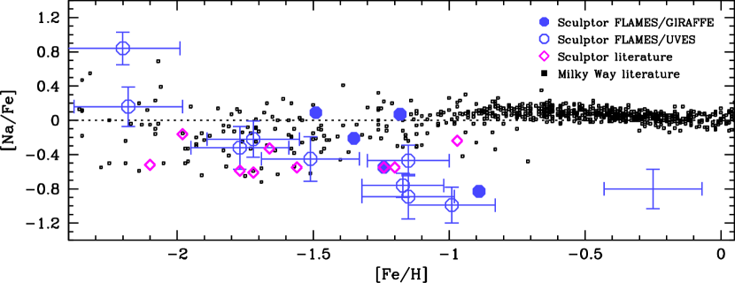
Figure 8: [Na/Fe] as a function of [Fe/H] for stars in Sculptor and the Milky Way. The blue circles are Sculptor stars from this work, GIRAFFE (filled) and UVES (open). Representative error bars for the GIRAFFE data is shown in blue (bottom right corner). Magenta open diamonds are previously published Sculptor stars, and the Milky Way is shown with small black squares. References: Sculptor: Shetrone et al. 2003; Geisler et al. 2005; Frebel et al. 2010; Starkenburg et al. 2013; Skúladóttir et al. 2015b; Simon et al. 2015; Jablonka et al. 2015. Milky Way: Venn et al. 2004 compilation; Nissen & Schuster 2010.

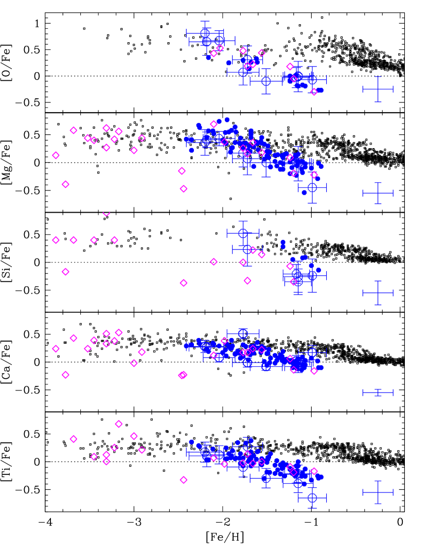
Figure 9: Abundance ratios for $\alpha$-elements as a function of [Fe/H] for Sculptor and the Milky Way. Symbols and Sculptor references are the same as in Fig. 8. Milky Way: Fulbright 2000 (Si); Carretta et al. 2000 (O); Nissen et al. 2002 (O); Reddy et al. 2003, 2006 (Si); Cayrel et al. 2004 (O, Mg, Si, Ca, Ti); Venn et al. 2004 compilation (Mg, Ca, Ti); Bensby et al. 2005 (O, Si); García Pérez et al. 2006 (O); Ramírez et al. 2007 (O); Nissen & Schuster 2010 (O, Si, Ca, Ti). Only O abundances derived from the [O I] line were included.

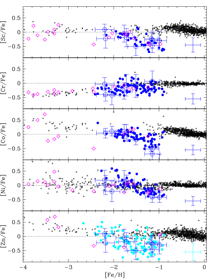
Figure 10: Abundance ratios for iron-peak elements as a function of [Fe/H] for Sculptor and the Milky Way. Cyan filled circles at the bottom panel are Zn measurements for Sculptor from Skúladóttir et al. (2017) which include the stars in our GIRAFFE sample, and a representative error bar is also shown in cyan. Otherwise, symbols and Sculptor references are the same as in Fig. 8. Milky Way: Fulbright 2000 (Cr, Ni); Reddy et al. 2003, 2006 (Sc, Cr, Co, Zn); Venn et al. 2004 compilation (Ni); Cayrel et al. 2004 (Cr, Co, Ni, Zn); Nissen & Schuster 2010, 2011 (Cr, Ni, Zn); Ishigaki et al. 2013 (Zn), Bensby et al. 2014 (Zn), Barbuy et al. 2015 (Zn).

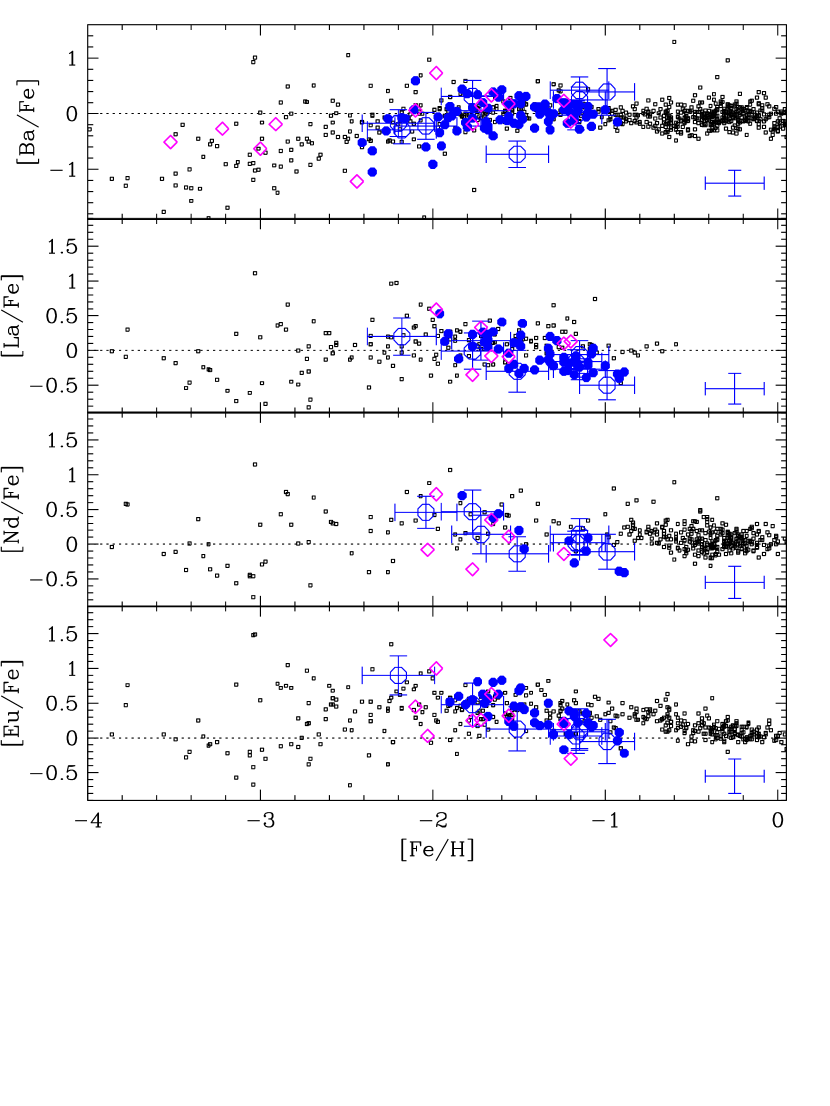
Figure 11: Abundance ratios for heavy elements as a function of [Fe/H] for Sculptor and the Milky Way. Symbols and Sculptor references are the same as in Fig. 8. Milky Way: Burris et al. 2000 (Ba, La, Nd, Eu); Reddy et al. 2003, 2006 (Nd); Venn et al. 2004 compilation (Ba, La, Eu); Simmerer et al. 2004 (La, Eu); François et al. 2007 (Ba, La, Nd, Eu).

5.2 The odd elements Na and Al

The only Na I lines accessible in the GIRAFFE spectral range are the Na i doublet at 6154 and 6161 Å. In our sample these lines are very weak and only detectable in a few stars, as shown in Fig. 8. With the larger wavelength coverage of UVES, more lines were accessible, see Table C. The [Na/Fe] abundance ratios seem to be slightly higher in the GIRAFFE sample compared to UVES, however, no systematic difference was found in abundance analysis from different Na lines in the UVES spectra. One possible reason for this offset could be that the lines are close to the detection limit in the GIRAFFE spectra, so only detected when the Na abundance tends to be high.

Two Al I lines, at 6696 and 6699 Å, were covered both by the UVES wavelength range and the HR15 setting in GIRAFFE. These very weak lines were only reliably detected in one GIRAFFE spectrum, ET0137, the most metal-rich star in our sample, with $\text{[Al/Fe]}=-0.35\pm 0.27$, and in none of the UVES spectra.

5.3 The $\alpha$-elements

The O, Mg, Si, Ca and Ti abundances, are shown in Fig. 9. With the exception of Si, GIRAFFE and UVES measurements are in very good agreement. In the case of Si, the GIRAFFE results are systematically shifted to higher abundance. This is the consequence of the line list, as only one Si I line, at 6245 Å, is accessible with the GIRAFFE spectra, while the line most commonly used for the UVES spectra is at 5685 Å. In the UVES star ET0143 both of these lines were measured, but the redder one gave a result $+0.3$ dex higher compared to the one at 5685 Å, thus explaining this difference. In the case of O, Mg, Si, Ca, Ti, the scatter was tested and found compatible with measurement uncertainties.

5.4 Iron-peak elements

Abundance ratios of the iron-peak elements Sc, Cr, Co, Ni, and Zn to Fe are shown in Fig. 10. In all cases, GIRAFFE and UVES results are in very good agreement. The odd element Sc was measured using one relatively weak line at 6310 Å, and could thus only be measured for high S/N GIRAFFE spectra, and typically not at the lowest metallicities. The heaviest of the iron-peak, Zn, was measured with a line at 4810 Å in the UVES spectra. No Zn line was available with the GIRAFFE wavelength coverage of this work. However, Zn was measured from GIRAFFE spectra for $\approx$100 stars (85 overlapping with our sample) in Skúladóttir et al. (2017), see more detailed discussion therein. The scatter in the iron-peak elements was found to be compatible with measurement uncertainties. However, there is a statistically significant correlation between the offsets from the mean trends in Ni and Zn, see further discussion in Skúladóttir et al. (2017).

5.5 Heavy elements

Four heavy elements were measured, Ba, La, Nd and Eu, see Fig. 11. The GIRAFFE and UVES results are in good agreement for all four elements. Unlike the iron-peak and $\alpha$-elements, the scatter exceeds what is expected from measurement uncertainties for Ba. The lighter $n$-capture element Y was measured in the UVES sample and for four stars in the GIRAFFE samples, but this will be published with more Y measurements from complementary observations in the GIRAFFE HR7A setting in Skúladóttir et al. (in prep.). Comparison of our Y measurement in ET0097 with that of Skúladóttir et al. (2015b) is done in Appendix A along with other elements for this star.

5.5.1 Comparison with intermediate resolution spectroscopy

A large number of stars (376) in the central field of Sculptor has previously been observed using Keck DEIMOS intermediate resolution spectra (Kirby et al. 2009, 2011). Overall, their results show similar trends to those presented here. However, there are also some significant discrepancies. A larger scatter in abundance ratios is observed in the the Keck DEIMOS data (as expected from spectra of lower resolution and S/N), but there are also differences in trends, especially at the lowest metallicities. When all the Kirby et al. (2009, 2011) data is considered, no knee in the [$\alpha$/Fe] abundance ratios is observed, however, it does become visible when only their most reliable measurements are used. For a more detailed discussion of this, see Appendix B.

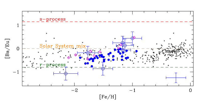
Figure 12: Abundance ratios of Ba to Eu with [Fe/H], as tracers of the $s$- to $r$-process contributions to the heavy elements in Sculptor. The dashed lines show the solar [Ba/Eu] (orange), as well as the pure $r$-process (green) and pure $s$-process (red), from Bisterzo et al. (2014). Symbols and Sculptor references are the same as in Fig. 8. Milky Way: Burris et al. 2000; Venn et al. 2004 compilation; François et al. 2007.

6 Sculptor, a textbook galaxy

In many ways, the Sculptor dSph can be thought of as the ideal galaxy to study chemical evolution. It is small enough not to have the complicated structure of the Milky Way (bulge, thin/thick disks, halo), but large enough so that statistically significant samples of stars can be observed with HR spectroscopy, as presented here. It is a well studied galaxy, with a relatively simple star formation history, with a peak of star formation at the earliest times, which then steadily decreased until $\sim 6$ Gyr ago (de Boer et al. 2012), when star formation stopped. Thus its entire stellar population is old, dominated by stars of ages $>10$ Gyr. Sculptor can therefore be seen as a ‘textbook’ galaxy, the ideal system to empirically witness chemical evolution reveal itself, from the earliest times to well after SN type Ia and intermediate-mass stars started contributing the metal enrichment.

6.1 Abundance trends in Sculptor

The chemical abundance ratios [X/Fe] as a function of [Fe/H] in Sculptor are significantly different from those observed in the Milky Way, see Figs. 8, 9, 10, and 11. This suggests differences in the chemical enrichment histories of these two galaxies.

6.1.1 General abundance trends

Both in Sculptor and the Milky Way, supersolar values of $\text{$[\alpha$/Fe]}>0$ are observed at the lowest metallicities. This is consistent with initial pollution only from SNe type II, which explode on short timescales, $\approx 10^{6}-10^{7}$ yr, and create large quantities of $\alpha$-elements, $\text{[$\alpha$/Fe]}>0$ (e.g. Nomoto et al. 2013). After 1-2 Gyr, SN type Ia start to significantly contribute to the chemical evolution of each system, releasing primarily Fe and other iron-peak elements (e.g. Iwamoto et al. 1999). This results in a knee in the [$\alpha$/Fe] abundance ratios, which start to decrease as the bulk of SNe type Ia start to contribute. In the Milky Way, this happens at relatively high metallicities, $\text{[Fe/H]}>-1$, but as Sculptor is a much smaller galaxy, with less efficient star formation, the gas is only enriched until $\text{[Fe/H]}\approx-1.8$ before the knee is observed, and the [$\alpha$/Fe] ratios start to decrease. Furthermore, the evolution and state of the gas in the galaxy will also affect how efficiently new metals are recycled into stars, ad might thus also influence the position of the knee (e.g. Lanfranchi & Matteucci 2007; Vincenzo et al. 2016; Côté et al. 2017; Romano & Starkenburg 2013; Revaz & Jablonka 2012).

The subsolar ratios of [$\alpha$/Fe], seen at the highest metallicities in Sculptor, are typically not observed in the Milky Way disks or halo, see Fig. 9. As star formation declined in Sculptor, the frequency of SN type II gradually decreased. Due to the delayed timescales of SN type Ia, however, their frequency at each time step is set by the higher star formation rate earlier on (typically 1-2 Gyr before). This could explain why the ratio of SN type Ia to type II in the later stages of the chemical evolution of Sculptor is relatively high (e.g. Lanfranchi & Matteucci 2003). In the Milky Way disk, on the other hand, the contribution from SN type Ia has always been together with a continuous contribution of SN type II, and therefore the observed [$\alpha$/Fe] ratios are not as low. The slope of [$\alpha$/Fe] with [Fe/H] is therefore also steeper in Sculptor compared to the Milky Way, showing a very clear and unobscured signal of an increasing SN type Ia contribution.

A similar declining trend can also be seen in Na and some of the iron-peak elements: Sc, Ni, Co and Zn (see Figs. 8 and 10). This indicates that the fraction of these elements to iron, [X/Fe], is higher in SN type II than in SN type Ia at these metallicities in Sculptor. In the case of Na, some production from AGB stars is also expected (e.g. Karakas & Lattanzio 2014). However, considering the strong NLTE effects for Na lines in metal-poor giants (up to $\gtrsim 0.5$ dex; e.g. Andrievsky et al. 2007), we advice against drawing strong conclusions for our limited number of LTE measurements of Na in Sculptor (see Fig. 8).

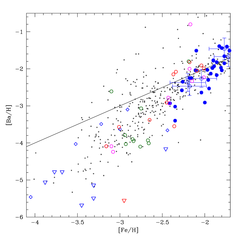
Figure 13: [Ba/H] as a function of [Fe/H] in dSph galaxies. Sculptor is depicted with blue circles: GIRAFFE (filled); UVES (open with error bars). Literature samples for $\text{[Fe/H]}\leq-2$: Sculptor in blue open circles (Shetrone et al. 2003; Geisler et al. 2005; Frebel et al. 2010; Starkenburg et al. 2013; Simon et al. 2015; Jablonka et al. 2015); Draco in red (Shetrone et al. 2001; Cohen & Huang 2009; Tsujimoto et al. 2017); Sextans in green (Tafelmeyer et al. 2010; Aoki et al. 2009); and Ursa Minor in magenta (Shetrone et al. 2001; Cohen & Huang 2010). Inverted triangles indicate upper limits. Black points are Milky Way halo stars (Burris et al. 2000; Venn et al. 2004, compilation; Barklem & Aspelund-Johansson 2005; François et al. 2007). The line is $\text{[Ba/H]}=\text{[Fe/H]}$.

6.1.2 Abundance trends of the heavy neutron-capture elements

The abundances of the heavy elements Ba, La, Nd, and Eu with [Fe/H] are shown in Fig. 11. These elements are created in the main rapid ($r$) and slow ($s$) neutron-capture processes.

The heavy element Eu is mainly formed in the $r$-process, which produces more than 94% of the Eu in the Sun (Bisterzo et al. 2014). The $r$-process requires high-energy, neutron-rich environments (e.g. Sneden et al. 2008) typically associated with the late evolution of massive stars, such as neutron star mergers (e.g. Rosswog et al. 1999; Wanajo et al. 2014; Ishimaru et al. 2015); high energy winds accompanying core-collapse SNe (Woosley et al. 1994; Qian & Wasserburg 2003; Wanajo et al. 2001; Wanajo 2013); or magneto-hydrodynamical explosions of fast rotating stars (Winteler et al. 2012). As measurements become challenging at the lowest metallicities, not much can be said about [Eu/Fe] at $\text{[Fe/H]}<-2$ in Sculptor. At higher metallicities, there is a decreasing trend of [Eu/Fe] with [Fe/H], similar to that of [$\alpha$/Fe]. This indicates that the $r$-process at these times and metallicities, was not sufficient to counteract the added contribution to Fe from SN type Ia.

Conversely, the $s$-process dominates the production of Ba in the solar system, (85%, Bisterzo et al. 2014). The $s$-process occurs in low mass ($M\lesssim 4$ M_⊙) AGB stars (Travaglio et al. 2004), and thus enters the evolution with a delay of at least $\sim$1 Gyr after the onset of star formation. At the earliest times in the Milky Way halo, the production of Ba is therefore dominated by the $r$-process. Early in the chemical evolution of Sculptor, $\text{[Fe/H]}\lesssim-1.8$, the [Ba/Fe] abundance ratios show a very large scatter, exceeding measurement uncertainties, with a subsolar mean value. Around $\text{[Fe/H]}\gtrsim-1.8$, the scatter in [Ba/Fe] decreases, and a plateau is reached around the solar value, in spite of the added Fe from SN type Ia at the same metallicities.

The relative $s$- to $r$-process contributions to the chemical enrichment of neutron-capture elements can be traced by [Ba/Eu], as is shown in Fig. 12. At the lowest metallicities in Sculptor, [Ba/Eu] is consistent with the $r$-process being the dominant production site of the neutron-capture elements. But as AGB stars start to contribute, the $s$-process gradually becomes more important, until at the highest metallicities solar or even supersolar ratios of [Ba/Eu] are reached. A similar trend appears at a higher metallicity in the Milky Way disk compared to Sculptor (analogous to the knee in [$\alpha$/Fe]). In this context, the rise of [Ba/Fe] in Sculptor (see Fig. 11) is clearly associated with the onset of the $s$-process. This rise in [Ba/Fe] happens at slightly higher metallicities in Sculptor than in the Milky Way halo. This was noted already by Tolstoy et al. (2009), and is a feature shared with other dSph galaxies (e.g. Shetrone et al. 2001, 2003), although Sculptor is currently the galaxy that best samples the relevant metallicity regime ($\text{[Fe/H]}<-2$), together with Draco (Tsujimoto et al. 2017).

The other two elements in Fig. 11, La and Nd, are more evenly created by the $s$- and $r$-processes (75% and 58% of the solar La and Nd, respectively, come from the $s$-process, according to Bisterzo et al. 2014). In the metallicity regime where the weak La and Nd lines could be measured ($\text{[Fe/H]}>-2$), the results indicate a slowly decreasing trend of [La/Fe] and [Nd/Fe]. This can be understood as being caused by the added SN type Ia contribution to Fe in this metallicity range, partially compensated by the $s$-process.

The recent detection of the neutron-neutron star merger, GW170817 by the LIGO team (Abbott et al. 2017) and its ultraviolet, optical and infrared emission confirm neutron star (NS-NS) mergers as significant production sites for the $r$-process (Chornock et al. 2017; Cowperthwaite et al. 2017; Drout et al. 2017; Pian et al. 2017; Villar et al. 2017). But the question still remains, whether other proposed $r$-process sites also play a significant role. The dSph galaxies may be the best environment to figure out the dominant source(s) for their production. A wide range of works have examined the possibility that the enrichment of mini-halos by neutron star mergers are responsible for the large [$r$/Fe] dispersion in the Milky Way halo. The rare neutron star merger going off in a mini-halo would pollute it entirely, to a high level (e.g. Ji et al. 2016a, b) while others would hardly see any (e.g. Tsujimoto & Shigeyama 2014; Hirai et al. 2017).

Tsujimoto et al. (2017) examined the absolute [Eu/H] content of stars in the Draco dSph galaxy, and found them to align on two distinct plateaus, one high and one low, irrespective of their metallicity. They interpreted this as two separate discrete events, one that elevated the $r$-process elements to the level of the first plateau by producing a modest amount of $r$-process (which they associate to magneto-hydrodynamical explosion of a fast rotating star), and the second (a neutron star merger) which produced a much larger mass of $r$- process elements that were well distributed throughout Draco, elevating the level to the second plateau.

In Fig. 13, a sample of classical dSph galaxies show the run of [Ba/H] at $\text{[Fe/H]}<-2$, where the production of Ba is dominated by the $r$-process. When comparing Draco with other similar galaxies, it is not clear any more that this plateau-like behaviour of the $r$-process is a good description. In Sculptor, the [Ba/H] increase appears regular and does not follow steps. In Sextans and Ursa Minor, there are also no clear signs of a plateau either. Possibly these dSph galaxies are too large to suffer an extreme global enrichment as an UFD or a mini-halo might.

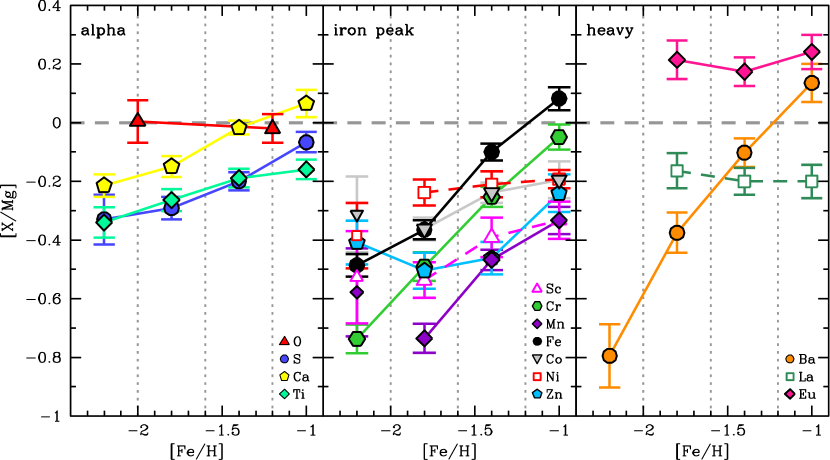
Figure 14: Abundance ratios [X/Mg] as a function of [Fe/H], in three panels for: O, S${}_{\text{NLTE}}$, Ca, Ti (left); Sc, Cr, Mn, Fe, Co, Ni, Zn (middle); and Ba, La, Eu (right). Data points including ¡10 stars (in all cases at the lowest metallicity bin) are not connected and are shown with small symbols for (number of stars): Sc (3), Mn (3), Co (4), and Ni (6). Elements only measured from very weak lines are shown with unfilled symbols (Sc, Ni, La). Error of the mean ($\sigma$/$\sqrt{N-1}$) is shown for each element with y-error bars. Dotted lines show the range of the [Fe/H] bins for all elements with the exception of O, where each data point covers two bins. References: Skúladóttir et al. 2015a (S); North et al. 2012 (Mn); Skúladóttir et al. 2017 (Zn).

6.2 The relative contributions of massive stars, SN type Ia, and AGB stars to chemical elements

For a quantitative comparison with theoretical nucleosynthetic yields, accurate NLTE (and preferentially 3D NLTE) abundances are required, as well as detailed calculations and/or models. However, with the data presented here we are able to make a qualitative evaluation of the relative contribution of different nucleosynthetic sites for each element in Sculptor. For our discussion we make four simplifying assumptions:

• SN type Ia and type II (and other core-collapse SN) are the main producers of the $\alpha$- and iron-peak elements.

• Mg is predominantly produced by SN type II, and the contribution from SN type Ia is negligible.

• For the main stellar population in Sculptor, the contribution of SN type Ia and the $s$-process is negligible at $\text{[Fe/H]}<-2$.

• For the elements discussed here, the SN type II yields and 3D NLTE corrections are not strongly metallicity dependent in the range $-2\lesssim\text{[Fe/H]}\lesssim-1$.

The first two assumptions are generally accepted, and supported both by theory and observations (e.g. Tsujimoto et al. 1995; Iwamoto et al. 1999; Kobayashi et al. 2006; Nomoto et al. 2013). Furthermore, the second one is also supported by our own data, as [Mg/Fe] shows the steepest negative slope with [Fe/H] (see Fig. 9), indicating very little contribution from SN type Ia. The third assumption is safely adopted as there is no evidence of SN type Ia nor the $s$-process in the measured abundance ratios in Figs. 8-11, at the lowest metallicities. The last assumption is justified in part by theoretical yields, which do not predict a strong metallicity dependence for the elements in question at these metallicities (Kobayashi et al. 2006). In addition, observations in the Milky Way generally show flat trends of [X/Fe] in the range $-2\lesssim\text{[Fe/H]}\lesssim-1$ (see Figs. 9 and 10), where SNe type II are believed to dominate the metal production, thus making strongly metallicity dependent yields or NLTE-effects unlikely overall. In a few cases, assumption 4) might not hold completely, due to sensitivity to 3D and/or NLTE effects, but for the majority of elements this should be a reasonable approximation for our purposes.

The abundance measurements shown in Fig. 9-11 and listed in Table 11 are divided into bins in [Fe/H] and the average of [X/Mg] in each bin are shown in Fig. 14. From our assumptions it directly follows that the abundance ratios at the lowest metallicities, $\text{[Fe/H]}<-2$, in Fig. 14 are direct measurements of the SN type II contribution to each element in question. Furthermore, if SNe type II were the only source of metals in Sculptor, all elements would show completely flat trend of [X/Mg] with [Fe/H]. Any increase in [X/Mg] with [Fe/H] therefore indicates a contribution from other sources (which do not affect the Mg abundance). In the case of $\alpha$- and iron-peak elements this is indicative of contributions from SN type Ia, while for the heavy elements this shows the effects of the $s$- and/or $r$-processes.

6.2.1 $\alpha$-elements

In the left panel of Fig. 14, the [$\alpha$/Mg] ratios are shown for O, Ca and Ti from this work, as well as NLTE-corrected S abundances from Skúladóttir et al. (2015a). In the case of O, stars are binned in two bins instead of four because of lack of data (see Fig. 9). As already shown in Skúladóttir et al. (2015a); Skúladóttir et al. (2018), the $\alpha$-elements in Sculptor do not all have constant ratios with respect to each other as a function of [Fe/H]. The only element with a flat trend is [O/Mg], indicating that the contribution to O by SN type Ia is negligible. For S, Ca, and Ti, on the other hand, the [$\alpha$/Mg] increases with added SN type Ia contribution in Sculptor. This is consistent with theoretical SN type Ia yields which predict almost no O, but non-negligible yields of the heavier $\alpha$-elements (e.g.Tsujimoto et al. 1995; Iwamoto et al. 1999).

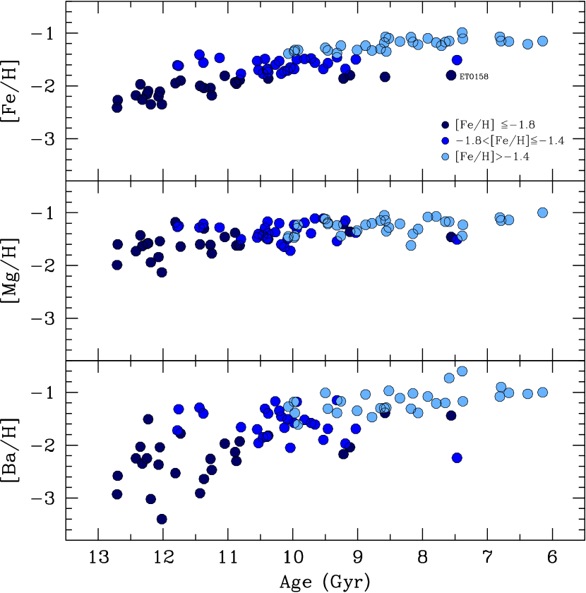
Figure 15: Abundances of Sculptor stars as a function of age for [Fe/H], [Mg/H] and [Ba/H]. Colours indicate the metallicity: most Fe-poor stars, $\text{[Fe/H]}\leq-1.8$, are dark blue; blue are $-1.8<\text{[Fe/H]}\leq-1.4$; and most Fe-rich are light blue, $\text{[Fe/H]}>-1.4$.

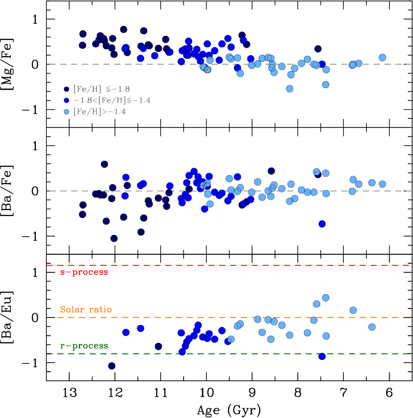
Figure 16: Abundance ratios, [Mg/Fe], [Ba/Fe], and [Eu/Ba] in Sculptor stars as a function of age. Red, orange, and green dashed lines in the bottom panel show the value of the $s$-process, the solar ratio, and $r$-process respectively (Bisterzo et al. 2014). Blue colours are the same as in Fig. 15.

6.2.2 Iron-peak elements

The iron-peak elements: Sc, Cr, Fe, Co and Ni from this work, and Mn from North et al. (2012), and Zn from our UVES data and Skúladóttir et al. (2017); are shown in the middle panel of Fig. 14. The elements Fe and Cr show very steeply increasing slopes with [Fe/H], indicating a very efficient production of these elements by SN type Ia. The same is true for Mn, with the possible exception of the most metal-poor data point, which only includes 3 stars, as measuring Mn becomes challenging at these metallicities. However, overall, the slopes of Mn, Fe, and Cr are very similar, and both [Cr/Fe] and [Mn/Fe] show a fairly flat trend with [Fe/H] (see Fig. 10 and North et al. 2012). Thus, [Mn/Fe] and [Cr/Fe], seem to be very similar in the yields of SN type II and type Ia. This is also seen in the Milky Way, where populations which separate into high- and low-$\alpha$ (and thus smaller and larger SN type Ia contributions) at similar metallicities ($-1.6\lesssim\text{[Fe/H]}\lesssim-0.8$) do not show such differences neither in [Cr/Fe] nor [Mn/Fe] (Nissen & Schuster 2010, 2011).

The light, odd, iron-peak element Sc also shows a very significant contribution from SN type Ia. However, there is a clear separation in atomic number, as the elements heavier than iron, Co, Ni, and Zn, all show only moderate or no contribution from SN type Ia. We advise slight caution for interpreting the quantitative trends of Sc and Ni as these elements are only measured from very weak lines, in the regime where distinguishing between upper limits and actual detections becomes challenging. This would result in slightly underestimate the increase of [X/Mg] with [Fe/H], but no drastic changes are expected.

These combined results of the iron-peak elements (in particular the small contribution from Ni) seem to indicate a dominant contribution of low-metallicity SN type Ia of sub-Chandrasekhar-mass explosions of white dwarfs (Sim et al. 2010; McWilliam et al. 2018). In the study of Nissen & Schuster (2010, 2011), a similar relation was found where both Ni and Zn correlated with the high and low $\alpha$-abundances, indicating less contribution from SN type Ia compared to the lighter iron-peak elements. Unfortunately Co was not included in their study. At higher metallicities in the Milky Way this correlation is less clear in the case of Ni (Mikolaitis et al. 2017). But the SN type II yields of all these elements, Co, Ni and Zn are predicted to be quite metallicity dependent at $\text{[Fe/H]}>-1$ (Kobayashi et al. 2006), making any interpretation not very straightforward. The case of Zn is discussed in detail in Skúladóttir et al. (2017), but both theory and observations are consistent with Zn not being significantly produced in SN type Ia.

6.2.3 Heavy neutron-capture elements

The heavy elements Ba, La and Eu over Mg are shown in the right panel of Fig. 14. The sharp increase in [Ba/Mg] with [Fe/H] results from an added production of Ba by the $s$-process, which happens on similar timescales to SN type Ia. The element Eu is mainly produced by the $r$-process, however, the lack of data at the lowest metallicities prevents us from drawing strong conclusions regarding Eu at the earliest epochs. At the higher metallicities in Sculptor, $\text{[Fe/H]}>-2$, [Eu/Mg] is constant. This does not necessarily mean that there is no increase in both these elements. Indeed, from metallicities $-2<\text{[Fe/H]}<-1.6$ to $\text{[Fe/H]}>-1.2$ there is an increase of $0.19\pm 0.11$ dex in [Eu/H], and a comparable increase in [Mg/H] of $0.24\pm 0.08$. The constant value of [Eu/Mg], however, excludes any significant time delay in the production of Eu compared to Mg on the order of $\gtrsim$1 Gyr.

The heavy element La is predicted to be produced both in the $s$- and $r$-processes (75% of the solar La is contributed by the $s$-process, according to Bisterzo et al. 2014). However, the contribution from the $s$-process is not obvious from Fig. 14. The most metal-poor [La/Mg] point only includes 5 stars, and is furthermore likely to be biased towards higher values, as the line is only measurable when the La value is high. But when the three metal-rich bins are considered, there is no clear trend of added contribution from the $s$-process to this element. However, these La abundances come from very weak lines so the mean [La/Mg] could be overestimated at the lowest metallicities. The details of the trends of the heavy neutron capture elements, along with new measurements for this stellar sample will be discussed in more detail in Skúladóttir et al. in prep.

6.3 Evidence for top-light IMF?

The Sagittarius dSph galaxy has been shown to be more deficient in hydrostatic $\alpha$-elements (O, Mg), compared to the explosive $\alpha$-elements (Si, Ca, Ti) at the highest metallicities, i.e. $\text{[Ca/Mg]}\approx+0.2$ (McWilliam et al. 2013; Hasselquist et al. 2017). In addition, very high abundances of $\text{[Eu/Mg]}_{r}\approx+0.4$ are observed (when Eu has been corrected for contribution from the $s$-process). The authors suggest that these combined results could be explained by a top-light initial mass function (IMF) in Sagittarius, missing the most massive supernovae, whose yields are relatively rich in the hydrostatic $\alpha$-elements.

As is shown in Fig. 14, these high values of [Ca/Mg] and [Eu/Mg] are not seen in our Sculptor data, even at the highest metallicities. However, there is a clear increasing trend of [S,Ca,Ti/Mg] with increasing [Fe/H]. This trend is difficult to explain with a top-light IMF as it requires either the IMF to change over time, or the yields of SN type II to be very metallicity dependent, which is not seen in the Milky Way at the same metallicities (see Fig. 9). At the lowest metallicities in Sculptor, $\text{[Fe/H]}<-2$ where the contribution from SN type Ia is negligible, all abundance ratios [$\alpha$/Fe] are consistent with what is observed in the Milky Way halo, showing no signs of differences in the IMF. Finally we note that an increase of e.g. [S/O] with [Fe/H] is also seen in the Milky Way disk at $\text{[Fe/H]}>-1$ where the contribution from supernovae type Ia is significant (see Skúladóttir et al. 2018 (Appendix) and references therein), thus making the origin of this trend very clear. We therefore conclude that our data shows no convincing evidence for a top-light IMF in the Sculptor dSph.

Alternatively, instead of different IMF, it is not clear how well the IMF is sampled in a small system with a low star formation rate (e.g. Tolstoy et al. 2003). However, if Sculptor is suffering from incomplete IMF sampling, the effect is small enough to be hidden within our measurement uncertainties. Smaller systems could a better place to witness the effects of incomplete IMF sampling.

6.4 Timescales in Sculptor

A detailed star formation history for Sculptor was derived from deep CMD covering the whole spatial extent of the galaxy (de Boer et al. 2012), while using the observed metallicity distribution of Sculptor as a constraint (Battaglia et al. 2008b; Kirby et al. 2011; Starkenburg et al. 2010). In this work, de Boer et al. (2012) also selected isochrones to derive ages of individual RGB stars, using their magnitude, colour, [Fe/H] and [$\alpha$/Fe]. This technique results in relatively low uncertainties on the ages, $\Delta\text{age}\approx\pm 1.8$ Gyr on average for our sample.

The elemental abundances of Fe, Mg, and Ba in Sculptor all have differences in their behaviour with age, as shown in Fig. 15. The slope of [Fe/H] with age is steeper compared to that of [Mg/H], as it traces both the contribution of type II and type Ia SNe, while the increase in Mg with time is only contributed by SN type II (e.g. Iwamoto et al. 1999; Kobayashi et al. 2006; Nomoto et al. 2013). The neutron-capture element Ba shows a very large scatter at the earliest times, $>$11 Gyr ago, exceeding both measurement uncertainties, and that of Fe and Mg. But around $\sim$11 Gyr ago, the main $s$-process became dominant and the scatter decreased. The large scatter at the earliest epoch is associated to the $r$-process, which does not trace normal SN type II production of $\alpha$-elements or iron at these times/metallicites (see Sec. 6.1.2).

The abundance ratios [Mg/Fe], [Ba/Fe] and [Ba/Eu] with age are depicted in Fig. 16. As shown in de Boer et al. (2012), [Mg/Fe] has a well defined decreasing trend with age, consistent with the contribution of SN type Ia becoming more important with time. Similar to [Ba/H], [Ba/Fe] has a large scatter at the earliest times. The bottom panel of Fig. 16 shows the relative ratios of the $s$- and $r$-processes with the [Ba/Eu] ratio. Similar to what is shown in Fig. 12, [Ba/Eu] at the earliest times is consistent with the $r$-process dominating the production of the heavy elements in Sculptor, but as time passes, the $s$-process becomes more significant.

Comparing all three panels, as well as Fig. 9, 11 and 12, seems to indicate that the timescales of the $s$-process and SN type Ia in Sculptor are comparable. The current dearth of Eu measurements at the oldest ages however prevent us from dating precisely the onset of the $s$-process. The fact that the high [Ba/Fe] dispersion diminishes at the same time as the [Ba/Fe] reaches the solar value, $\sim$11 Gyr ago is probably the best trace of the $s-$process onset.

7 Conclusions

We have analysed high-resolution VLT/GIRAFFE and VLT/UVES spectra of 99 red giant branch stars in the Sculptor dwarf spheroidal galaxy, to measure the abundances of $17$ chemical elements made up by different nucleosynthetic channels: Li, Na, $\alpha$-elements (O, Mg, Si, Ca Ti), iron-peak elements (Sc, Cr, Fe, Co, Ni, Zn), and $r$- and $s$-process elements (Ba, La, Nd, Eu). The sample stars have a wide range in metallicity, $-2.3<$ [Fe/H] $<-0.9$, populating the whole metallicity distribution of the galaxy with the exception of the very low-metallicity tail, which has been studied elsewhere (Tafelmeyer et al. 2010; Frebel et al. 2010; Starkenburg et al. 2013; Jablonka et al. 2015; Simon et al. 2015). Armed with these high-precision elemental abundances we have examined the details of how metal-enrichment proceeds in a small galaxy with a single-peaked star formation which lasted several Gyr before fading away. In many ways, the abundance ratios evolve with metallicity and with time according to expectations from basic nucleosynthetic prescriptions, making Sculptor a textbook galaxy to study chemical evolution.

Our dataset establishes with reasonably good precision, and on statistical grounds, a number of chemical properties of Sculptor that stem naturally from the star formation history of this system:

• There is a marked decrease in [$\alpha$/Fe], which starts at the Galactic halo plateau value for low [Fe/H] and decreases steadily after a knee, to sub-solar [$\alpha$/Fe]  for high [Fe/H], in agreement with expectations given the star formation history of Sculptor, with a dominance of the products of massive stars dying as core-collapse supernovae at early times, and an onset of SN Ia as early as $\sim$12 Gyr ago.

• The position of the knee, around $\text{[Fe/H]}\approx-1.8$, occurs at much lower metallicity than in the Milky Way disks (e.g. Bensby et al. 2014) or bulge (e.g. Hill et al. 2011; Gonzalez et al. 2011), in agreement with the lower star formation efficiency in Sculptor. The position of the knee can also be affected by the ability of the galaxy to retain freshly formed metals (e.g. Lanfranchi & Matteucci 2007; Vincenzo et al. 2016; Côté et al. 2017), and more generally the origin, state and fate of the gas in these galaxies, where feedback plays a role not only in regulating star formation but also gas enrichment (e.g. Revaz & Jablonka 2012).

• The products from low-mass AGB stars, as traced by the $s$-process, are also incorporated in the chemical evolution of Sculptor on a longer timescale than massive stars, more similar to that of SN type Ia.

• Except for neutron-capture elements in the early phases of the evolution, the scatter around mean trends in Sculptor for [Fe/H]$>-2.3$ is extremely low, compatible with observational errors. In addition, there is little evidence for scatter in the age-metallicity relations. This calls for an efficient mixing of metals in the gas at all times, at least in the last $\sim$12 Gyr. This has inspired modes that include the mixing (Revaz & Jablonka 2018) or diffusion (e.g. Escala et al. 2018) of metals in the galaxy.

As the origin of Sculptor chemical enrichment is quite straightforward, we can also refine the empirical constraints on nucleosynthesis processes:

• We estimated the relative importance of SN Ia contributions to individual iron-peak and $\alpha$ elements. The most important contribution of SN type Ia is to the iron-peak elements: Fe, Cr and Mn; however, there is also a modest but non-negligible contribution to both the heavier $\alpha$-elements: S, Ca and Ti, and some of the iron-peak elements: Sc and Co. In Sculptor the lightest $\alpha$-elements (O and Mg) and the heaviest iron-peak elements (Ni and Zn) are consistent with having little or no contribution from SN type Ia.

• Sculptor also sheds light on the production of neutron-capture elements through the $r$-process channel, showing a gradual and regular enrichment by the main $r$-process all along the metallicity range, at odds with the idea that the $r$-process in dwarf galaxies would come from very rare events polluting gas to very high levels. This has been seen widely in classical dwarf spheroidal galaxies (e.g. Letarte et al. 2010; Lemasle et al. 2012, 2014), whereas smaller systems such as the ultra-faint dwarf galaxies seem to populate more extreme $r$- enhancements (e.g. Ret II, Ji et al. 2016a) or very low levels of $r$-products (e.g. Frebel et al. 2014; Ji et al. 2016c).

• The chemical evolution in Sculptor does not show signs of having significantly different initial mass function compared to the Milky Way.

The very earliest days of the Sculptor galaxy, however, are still poorly represented in our sample, in part because this sample was drawn from the inner 25’ radius of the system whose tidal radius is approximately 77’ (Mateo 1998), which badly samples the oldest and most metal-poor population of Sculptor (Tolstoy et al. 2004; Coleman et al. 2005; Clementini et al. 2005; Battaglia et al. 2008b; de Boer et al. 2012). Obtaining the detailed abundances of sizeable samples of red giants in Sculptor with $\text{[Fe/H]}<-2$, in particular in the range $-3<\text{[Fe/H]}<-2$, has the power to shed light on a variety of open questions on the earliest epochs of star formation, when [Fe/H] was possibly not yet a good proxy for time. This will be key to answering many open questions: the $r$-process production site and dispersion mechanism, the first traces of the $s$-process, nucleosynthesis -or the absence thereof- of massive stars in dwarf galaxies, the first star formation in a small dark matter halo and its relation to C-enrichment, among others.

graphystyleaa

Appendix A Verification of the abundance analyses

To ensure the accuracy of our abundance results from FLAMES/GIRAFFE spectra, six stars with detailed abundance determinations from UVES slit spectroscopy were reobserved: Scl-459, Scl-461, and Scl-482 from Shetrone et al. (2003), hereafter S+03; and Scl-195, Scl-770, and Scl-1446 from Geisler et al. (2005), hereafter G+05. In addition, the star ET0097 was discovered to be a carbon-enhanced metal-poor (CEMP-no) star, and thus reobserved by Skúladóttir et al. (2015b), hereafter Sk+15b, with UVES slit spectroscopy. The nature of the comparison with ET0097 is slightly different, as our GIRAFFE analysis does not account for CN molecular lines, which are present in the HR UVES spectra. The results for these stars, as well as their names for cross-identification, are listed in Table 5.

A.1 Equivalent width (EW) measurements

The FLAMES/GIRAFFE line strengths were determined from DAOspec, using the line list given in Table C. The FWHM given by DAOspec was consistent over all HR settings, see Table 6, as is expected for an RGB stellar sample at this resolution. The higher $\sigma$ in the HR15 setting results from lower number of available lines in this region. While DAOspec fits only Gaussian profiles to the spectral lines, the lower resolution of the GIRAFFE spectra results in line profiles that have an instrumental broadening that is well matched to a Gaussian over our EW measurement range (EW $\leq$ 300 mÅ).

The method used here is different from S+03 and G+05, where lines were measured individually using splot in IRAF, but the agreement in EW measurements is overall good. There were slight systematic offsets between this work and S+03, which can be traced directly to the S/N ratio of the spectra, and thus the continuum placement. For high S/N ratio spectra, the continuum level is clear; but as the S/N ratio lowers, DAOspec favours the centre of the noise, whereas the method adopted by S+03 sets the continuum slightly higher, at 2/3 the noise. Thus, the DAOspec EWs might be slightly and systematically smaller in low S/N ratio spectra. Our comparisons imply, however, that these offsets are within our EW measurement error estimates (worst case offset is $\leq 4$ mÅ while the minimum adopted EW error is 6 mÅ). Detailed comparisons with the G+05 data shows some EWs which are significantly stronger than our FLAMES/GIRAFFE measurements, particularly for ET0051/Scl-1446. Each of these lines has been examined in our GIRAFFE spectra for unrecognised blends, but none have been found. Overall, however, the agreement with S+03 and G+05 is within the adopted measurement errors.

Table 5: Comparisons of the derived stellar parameters and [Fe/H] with previously published UVES results.

Names	Teff	log g	vt	[Fe I/H]	[Fe II/H]	Teff	log g	vt	[Fe I/H]	[Fe II/H]	Ref.
	K		km s-1			K		km s-1
ET0071/Scl-482	4243	0.5	1.7	$-1.35\pm 0.14$	$-1.27\pm 0.16$	4400	1.10	1.70	$-1.24\pm 0.07$	$-1.26\pm 0.12$	Shetrone et al. 2003
ET0151/Scl-461	4281	0.6	1.7	$-1.77\pm 0.16$	$-1.70\pm 0.14$	4500	1.20	1.70	$-1.56\pm 0.07$	$-1.58\pm 0.12$	Shetrone et al. 2003
ET0389/Scl-459	4394	0.8	1.5	$-1.60\pm 0.22$	$-1.47\pm 0.20$	4500	1.00	1.65	$-1.66\pm 0.07$	$-1.65\pm 0.12$	Shetrone et al. 2003
ET0051/Scl-1446	3971	0.5	1.7	$-0.92\pm 0.12$	$-0.80\pm 0.33$	3900	0.00	2.30	$-1.20\pm 0.13$		Geisler et al. 2005
ET0113/Scl-195	4285	0.2	1.8	$-2.18\pm 0.19$	$-2.09\pm 0.14$	4250	0.20	1.80	$-2.10\pm 0.15$		Geisler et al. 2005
ET0141/Scl-770	4188	0.3	1.9	$-1.68\pm 0.15$	$-1.62\pm 0.13$	4075	0.00	1.90	$-1.72\pm 0.13$		Geisler et al. 2005
ET0097	4300	0.5	2.0	$-1.91\pm 0.16$	$-1.84\pm 0.26$	4383	0.75	2.25	$-2.03\pm 0.10$	$-1.86\pm 0.14$	Skúladóttir et al. 2015b

A.2 Stellar parameters

Table 6: The FWHM (mean and $\sigma$, per pixel) for the FLAMES/GIRAFFE settings, as determined by DAOspec ($1\leavevmode\nobreak\ \text{pixel}=0.05$ Å).

Setting	FWHM	$\sigma$
HR10	6.10	0.27
HR13	6.35	0.27
HR14	5.69	0.45
HR15	6.70	1.16

The effective temperatures, T_eff, were determined differently in S+03, G+05, and Sk+15b, and each differ from this analysis as well. S+03 used Fe i as a function of excitation potential, $\chi$, with a starting point based on (B-V) dereddened colour and assuming a metallicity from the star’s CMD location. G+05 adopted temperatures from (V-K) and (J-K) colours based on calibrations from Bessell et al. (1998). Sk+15b adopted photometric temperatures based on Ramírez & Meléndez (2005). S+03 and G+05 determined gravity, log g, using the same method as here, but ionisation equilibrium delivers gravities that are dependent on the adopted T_eff. In Sk+15b photometric gravities were used. Microturbulence velocities, v_t, were determined in all three papers by minimising the Fe I abundance dependency on observed equivalent widths, whereas here the expected line strength was used.

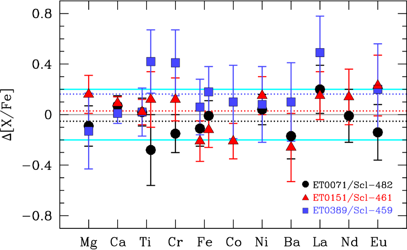
Figure 17: Abundance differences between our GIRAFFE analysis and S+03, $\Delta\text{[X/Fe]}=\text{[X/Fe]}_{\text{GIR}}-\text{[X/Fe]}_{\text{S+03}}$. In the case of Fe, $\Delta\text{[Fe/H]}$ is plotted instead. For Ti and Fe, the ionised species are plotted to the right. Dotted lines are the average abundance offsets for each star, while solid cyan lines show the expected GIRAFFE precision.

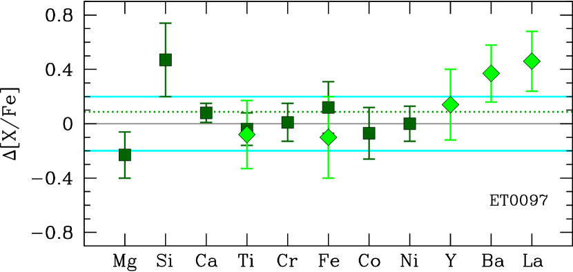
Figure 18: Same comparison as in Fig. 17 for ET0097 in Sk+15b. Neutral species are plotted with dark green squares, ionised with green diamonds. Lines are the same as in Fig 17.

A comparison of the atmospheric parameters for the seven stars, which overlap with S+03, G+05 and Sk+15b, is shown in Table 5. Temperatures in this work are slightly cooler than those determined by S+03 ($\Delta\text{T${}_{\rm eff}$}=-161\pm 42$ K), and warmer for the G+05 stars ($\Delta\text{T${}_{\rm eff}$}=+73\pm 32$ K). Accordingly, our gravities are lower than in S+03 ($\Delta\text{log\leavevmode\nobreak\ g}=-0.47\pm 0.19$) and higher than in G+05 ($\Delta\text{log\leavevmode\nobreak\ g}=+0.27\pm 0.20$). Microturbulence velocities agree within error bars, except for the coolest star of the G+05 sample where we find a microturbulence 0.5 km.s^-1 lower. In fact, for this cool star, the GIRAFFE spectra did not allow us to constrain v_t satisfactorily, which is reflected in a larger metallicity error. The only significant differences are therefore the slightly hotter S+03 temperature scale (and its correspondingly higher gravities). However, the resulting metallicities are compatible with those of S+03 and G+05 within the errors. For ET0097, T_eff, log g, v_t  and metallicity all agree within errorbars between our analysis and Sk+15b, indicating that the CN molecular lines were not a serious issue for this star at the resolution and wavelength range observed in this work.

Finally, DAOspec was used to measure all the spectral lines in the UVES spectra of S+03 to directly compare the different analyses. The agreement is very good over most of the EW range; however, the strongest lines are not well fit by Gaussian profiles at the resolution of UVES, and thus DAOspec underestimates the EWs by not fitting the damping wings. This is not a significant problem for the FLAMES/GIRAFFE spectra since the resolution is lower, and therefore the profile is dominated by the instrumental (gaussian) profile all the way to at least $\sim$200mÅ. More problematic is that some stars show a trend of increasingly disparate measurements with increasing line strength. This is more concerning because of the spectroscopic methods used to determine the stellar atmospheric parameters. For example, a trend of decreasing EW and thus decreasing resulting abundance in Fe i lines will mimic a higher microturbulence value, resulting in incorrect stellar parameters. Therefore, we conclude that at the higher resolution of the UVES spectra, DAOspec should not be used for spectral line measurements (at least above EW$\sim$120mÅ), however, it seems to be very well matched to the resolution of the FLAMES/GIRAFFE spectra.

A.3 Abundance trend

There are some differences in the stellar parameters adopted here compared to those of S+03, G+05, and Sk+15b (see Table 5), and the same is true for the model atmospheres, since all previous analyses used MARCS models (Gustafsson et al. 1975). The linelist and atomic data used here (see Table C) also differs slightly from that of S+03 and G+05, and significantly from Sk+15b. Finally, S+03 and G+05 used the LTE spectrum synthesis code MOOG (Sneden 1973) for abundance determinations, and in Sk+15b, the LTE code Turbospectrum (Plez 2012) was used, while here we use a different code, originally developed by Spite (1967).

To test how these slight differences affect the results, our FLAMES/GIRAFFE abundance measurements are compared to S+03 in Fig. 17. The agreement is excellent for most elements in all three stars. The elements with more discrepancy include Ti II and La II, which are both detected with very few (1-3) and very weak lines in the GIRAFFE spectra. Despite an offset in the Fe abundances in ET0151/Scl-461 (due to a 200 K difference in T_eff and 0.6 dex in log g), most relative element abundances are still in good agreement with S+03. The star ET0389/Scl-459 has the lowest S/N of the three (and among the lowest in the GIRAFFE sample) but still shows a rather good agreement for most species (10 of 13 elements) in common with S+03. Those in poor agreement are elements measured from weak lines, and typically have higher abundances from our analysis. This is the only star for which the overall abundance pattern is displaced, $<\Delta\text{[X/Fe]}>=+0.14$ over 13 elements.

The comparison of the CEMP-no star, ET0097, between this analysis and Sk+15b is shown in Fig. 18. The linelist used in Sk+15b is significantly different from the one used here, in particular as the UVES spectrum is missing the wavelength coverage offered by HR10, but includes both bluer and redder regions than available in our GIRAFFE spectra. Overall the agreement is excellent, with few notable exceptions. Like discussed in Section 4.3.2, the Si I line at 6244.5 Å, which is used for ET0097 in the GIRAFFE sample, gives systematically high Si abundances, with an offset of $\sim+0.30$ dex, explaining the discrepancy seen in Fig. 18. Out of the two Ba II lines in common with both analyses, 6141.7 and 6497.0 Å, the redder line is in agreement, while a significantly lower abundance is derived by Sk+15b for the bluer line. For Mg and La there are no overlapping lines used in these analyses, as stronger La II lines in the blue of the UVES spectrum are favoured. In the case of the GIRAFFE spectrum, La is determined from 2 very weak lines ($<30$  mÅ), close to our detection limit.

Appendix B Comparison with intermediate resolution spectroscopy

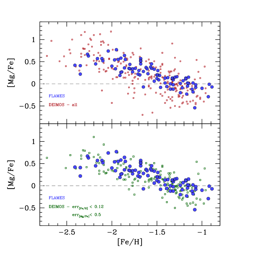
Figure 19: Comparison of [Mg/Fe] between our HR FLAMES results (blue cirles) and those of Keck DEIMOS (squares). Top panel shows all published measurements by Kirby et al. (2009, 2011) in red, while the bottom panel shows only the most reliable measurements, ($\text{err}_{\text{[Fe/H]}}<0.12$, and $\text{err}_{\text{[Mg/Fe]}}<0.5$) in green.

At present there is a large number of intermediate resolution, R $\sim\leavevmode\nobreak\ 5000-10000$, multi-object spectrographs that allow us to obtain detailed spectra of individual stars in nearby galaxies. One particular approach has made use of the entire extensive forest of small lines over a large wavelength range without significant individual detections, which are then compared to synthetic spectra rather than being measured individually (e.g Kirby et al. 2008).

The abundances of a range of elements (Fe, Mg, Ca, Si and Ti) were determined in this way for a large sample of 376 RGB stars in the centre of the Sculptor dSph using Keck DEIMOS spectra (Kirby et al. 2009, 2011). These lower resolution abundance measurements are compared to our HR FLAMES analysis in Fig. 19. As shown, the method applied by Kirby et al. (2009, 2011) can efficiently obtain a large sample of abundances, and shows the general trends in $\alpha$-element abundance ratios. Predictably, however, the precision is less than if individual lines can be accurately measured with HR and high S/N spectra. This is therefore not the best method to understand the scatter in abundance ratios, and, as we show here, it also may suffer from inaccuracies which increase with decreasing metallicity as many of the weak lines disappear.

From Fig. 19 it is evident that the overall picture changes if only the most reliable points from Kirby et al. (2009, 2011) are plotted. If all measurements are included, there is no change in the slope, so-called knee, in the [Mg/Fe] vs [Fe/H] in Sculptor, suggesting that Sculptor has had very early enrichment by SN Ia (Kirby et al. 2011). However, if only measurements with $\text{err}_{\text{[Fe/H]}}<0.12$ and $\text{err}_{\text{[Mg/Fe]}}<0.5$ are shown, the results become more consistent with present work, i.e. showing a knee in the distribution of measurements at $\rm[Fe/H]<-1.8$, which we interpret as the time when SN Ia start to contribute to the chemical enrichment, $\sim$1-2 Gyr after the onset of star formation (de Boer et al. 2012).

Appendix C Online tables

Table 7: GIRAFFE and UVES Target Stars in Sculptor. Stars considered non-members (NM) are noted, as well as stars with a different membership definition by Gaia.

Target	RA	DEC	V	I	J	K	vr	S/N	Gaia DR2 ID	RA PM$\pm$err	Dec PM$\pm$err	Comment
	J2000	J2000	mag	mag	mag	mag	km/s			mas/yr	mas/yr
ET0009	1 00 54.18	-33 40 14.60	17.149	15.835	14.743	13.882	95.77 $\pm$0.27	33	5027216583830257536	0.074 $\pm$0.100	-0.166 $\pm$0.090
ET0013	1 00 50.24	-33 36 38.20	17.335	16.121	…	…	105.07 $\pm$0.95	22	5027217820780833536	0.188 $\pm$0.099	0.070 $\pm$0.099
ET0024	1 00 34.04	-33 39 04.61	17.200	15.654	…	…	112.88 $\pm$0.37	40	5027220187306194048	0.217 $\pm$0.090	-0.095 $\pm$0.081	Gaia-NM
ET0026	1 00 12.76	-33 41 16.00	17.280	16.025	14.966	14.151	98.36 $\pm$0.30	51	5027218714133971712	0.022 $\pm$0.103	-0.178 $\pm$0.088
ET0027	1 00 15.37	-33 39 06.20	17.287	15.988	14.891	14.065	112.34 $\pm$0.18	51	5027219676206641152	0.201 $\pm$0.096	-0.070 $\pm$0.093
ET0028	1 00 17.77	-33 35 59.71	17.345	16.002	…	…	120.24 $\pm$0.22	43	5027221359833813504	0.076 $\pm$0.094	0.004 $\pm$0.090
ET0031	1 00 07.57	-33 37 03.89	17.457	16.262	15.239	14.508	115.05 $\pm$0.27	38	5027220019804016768	0.065 $\pm$0.112	-0.119 $\pm$0.120
ET0033	1 00 20.29	-33 35 34.51	17.495	16.295	…	…	108.68 $\pm$0.22	38	5027221359833858944	0.066 $\pm$0.113	-0.061 $\pm$0.102
ET0035	1 00 25.78	-33 30 25.41	17.692	16.543	…	…	120.24 $\pm$0.11	26	5027233969857854720	0.052 $\pm$0.128	-0.292 $\pm$0.126
ET0039	1 00 26.19	-33 31 38.79	17.788	16.680	…	…	119.71 $\pm$0.67	29	5027222184467596416	0.097 $\pm$0.143	-0.428 $\pm$0.131
ET0043	1 00 13.95	-33 36 39.20	17.847	16.674	15.620	14.831	110.17 $\pm$0.55	33	5027221428553291008	0.164 $\pm$0.133	-0.156 $\pm$0.128
ET0048	0 59 55.63	-33 33 24.61	16.890	15.806	…	…	120.53 $\pm$0.16	47	5027232870346158848	0.060 $\pm$0.083	-0.065 $\pm$0.076	Gaia-NM
ET0051	0 59 46.41	-33 41 23.50	17.304	15.857	14.681	13.722	108.48 $\pm$0.22	49	5027219298249516032	0.076 $\pm$0.096	-0.245 $\pm$0.089	Scl-1446
ET0054	0 59 56.60	-33 36 41.70	17.434	16.231	15.185	14.415	103.46 $\pm$0.18	41	5027231702115059328	0.024 $\pm$0.105	-0.165 $\pm$0.105
ET0057	0 59 54.21	-33 40 27.20	17.480	16.205	…	…	99.30 $\pm$0.43	44	5027219435688469376	0.154 $\pm$0.115	-0.133 $\pm$0.102
ET0059	0 59 38.11	-33 35 08.00	17.537	16.308	…	…	115.94 $\pm$0.19	40	5027232595468251136	0.049 $\pm$0.110	-0.049 $\pm$0.116
ET0060	0 59 37.74	-33 35 59.99	17.541	16.302	…	…	96.60 $\pm$0.20	42	5027232354950083840	0.192 $\pm$0.104	0.038 $\pm$0.105
ET0062	0 59 47.21	-33 33 36.90	17.608	16.451	…	…	105.03 $\pm$0.41	37	5027232801626681088	0.226 $\pm$0.118	-0.072 $\pm$0.115
ET0063	0 59 37.22	-33 37 10.50	17.608	16.339	15.195	14.347	109.41 $\pm$0.21	38	5027232183151393536	0.116 $\pm$0.115	-0.080 $\pm$0.109
ET0064	0 59 41.40	-33 38 47.00	17.615	16.387	15.339	14.480	113.32 $\pm$0.16	42	5027231358517676032	0.172 $\pm$0.116	-0.116 $\pm$0.108
ET0066	1 00 03.60	-33 39 27.10	17.607	16.402	…	…	118.64 $\pm$0.37	42	5027219779285853312	-0.145 $\pm$0.146	-0.118 $\pm$0.116
ET0067	0 59 37.00	-33 30 28.40	17.706	16.495	…	…	99.81 $\pm$0.35	35	5027236203240775680	0.074 $\pm$0.126	-0.073 $\pm$0.117
ET0069	0 59 40.46	-33 35 53.80	17.699	16.581	…	…	101.88 $\pm$0.76	35	5027232389309822464	-0.026 $\pm$0.126	-0.108 $\pm$0.120
ET0071	0 59 58.27	-33 41 08.70	17.679	16.479	15.410	14.618	106.50 $\pm$0.20	38	5027219160810565888	0.164 $\pm$0.139	-0.044 $\pm$0.115	Scl-H482
ET0073	0 59 53.99	-33 37 42.10	17.847	16.706	…	…	121.94 $\pm$0.43	35	5027231667755321728	0.024 $\pm$0.140	0.010 $\pm$0.130
ET0083	0 59 11.83	-33 41 25.30	17.476	16.297	15.295	14.528	122.15 $\pm$0.15	45	5003212527008328960	-0.011 $\pm$0.116	0.094 $\pm$0.111
ET0094	0 59 20.65	-33 48 56.60	17.136	15.789	…	…	119.40 $\pm$0.22	44	5003197752320843904	0.338 $\pm$0.106	-0.275 $\pm$0.097
ET0095	0 59 20.80	-33 44 04.79	17.210	15.985	14.961	14.135	109.47 $\pm$0.15	61	5003211427496707712	0.067 $\pm$0.095	-0.039 $\pm$0.102
ET0097	0 59 12.09	-33 46 20.80	17.266	16.132	15.104	14.305	105.40 $\pm$0.45	50	5003209778229298816	0.133 $\pm$0.100	-0.003 $\pm$0.098
ET0103	0 59 18.85	-33 42 17.31	17.599	16.383	…	…	115.98 $\pm$0.36	42	5003212355209640320	-0.122 $\pm$0.135	-0.238 $\pm$0.120
ET0104	0 59 15.14	-33 42 54.60	17.651	16.497	15.474	14.632	110.64 $\pm$0.23	43	5003212217770687360	0.077 $\pm$0.137	0.059 $\pm$0.125
ET0109	0 59 28.29	-33 42 07.20	17.118	15.643	…	…	102.50 $\pm$0.47	63	5003211942892781184	0.039 $\pm$0.082	-0.069 $\pm$0.076	Gaia-NM
ET0113	0 59 55.68	-33 46 40.10	17.233	16.019	14.943	14.177	122.63 $\pm$0.36	57	5003198783113034624	0.016 $\pm$0.097	-0.110 $\pm$0.084	Scl-195
ET0121	1 00 00.49	-33 49 35.80	17.512	16.397	…	…	113.94 $\pm$0.26	48	5003195518937893632	0.063 $\pm$0.119	-0.144 $\pm$0.103
ET0126	0 59 42.57	-33 42 18.10	17.563	16.302	…	…	102.71 $\pm$0.24	40	5003200054423348608	0.189 $\pm$0.116	-0.322 $\pm$0.112
ET0132	0 59 58.24	-33 45 50.80	17.723	16.563	15.485	14.704	101.61 $\pm$0.21	43	5003198886192249472	0.130 $\pm$0.129	-0.170 $\pm$0.117
ET0133	0 59 47.67	-33 47 29.50	17.814	16.589	15.518	14.659	111.82 $\pm$0.28	40	5003198439515638400	0.008 $\pm$0.133	-0.127 $\pm$0.120
ET0137	1 00 25.30	-33 50 50.79	17.109	15.651	…	…	114.49 $\pm$0.10	44	5027213525813501440	0.240 $\pm$0.083	-0.156 $\pm$0.076
ET0138	1 00 38.12	-33 48 16.90	17.212	15.917	14.854	14.029	110.18 $\pm$0.33	38	5027214006849837568	0.149 $\pm$0.098	-0.232 $\pm$0.082
ET0139	1 00 42.50	-33 44 23.50	17.208	15.841	14.707	13.796	91.09 $\pm$0.46	39	5027215999714657664	0.314 $\pm$0.093	-0.030 $\pm$0.086
ET0141	1 00 23.84	-33 42 17.40	17.333	16.047	…	…	120.43 $\pm$0.30	39	5027218542335286912	-0.004 $\pm$0.100	-0.263 $\pm$0.091	Scl-770
ET0147	1 00 44.27	-33 49 18.80	17.478	16.199	…	…	111.84 $\pm$0.48	21	5027167105806967296	0.122 $\pm$0.109	-0.208 $\pm$0.103
ET0150	1 00 22.98	-33 43 02.20	17.485	16.162	…	…	100.01 $\pm$0.15	37	5027215484318574848	0.036 $\pm$0.111	-0.112 $\pm$0.097
ET0151	1 00 18.29	-33 42 12.20	17.518	16.303	…	…	104.04 $\pm$0.58	41	5027218507975545984	0.152 $\pm$0.113	-0.165 $\pm$0.108	Scl-H461
ET0158	1 00 18.96	-33 45 14.80	17.677	16.600	15.672	14.954	111.04 $\pm$0.32	34	5027215003282241664	0.146 $\pm$0.130	-0.130 $\pm$0.116
ET0160	1 00 22.33	-33 50 24.00	17.714	16.508	…	…	112.67 $\pm$0.37	33	5027213731971930880	-0.024 $\pm$0.127	-0.088 $\pm$0.118
ET0163	1 00 24.63	-33 44 28.89	17.783	16.652	15.742	15.044	121.23 $\pm$0.26	37	5027215415599101824	-0.124 $\pm$0.136	-0.140 $\pm$0.121
ET0164	1 00 33.86	-33 44 54.40	17.796	16.697	15.717	14.993	112.71 $\pm$0.33	33	5027215239503594240	0.193 $\pm$0.141	-0.117 $\pm$0.121
ET0165	1 00 11.79	-33 42 16.89	17.786	16.568	…	…	113.17 $\pm$1.12	35	5027218679774236160	0.180 $\pm$0.142	-0.204 $\pm$0.124
ET0166	1 00 10.49	-33 49 36.90	17.829	16.678	…	…	117.43 $\pm$0.38	37	5003195381498941184	-0.003 $\pm$0.143	-0.187 $\pm$0.130
ET0168	1 00 34.32	-33 49 52.90	17.869	16.684	…	…	113.22 $\pm$0.52	29	5027213594532978304	-0.055 $\pm$0.142	-0.085 $\pm$0.133
ET0173	1 00 50.87	-33 45 05.20	17.213	15.714	14.490	13.562	103.59 $\pm$0.32	30	5027215690477068160	0.006 $\pm$0.091	-0.244 $\pm$0.084	Gaia-NM
ET0198	1 00 09.18	-33 36 09.40	17.924	16.814	…	…	119.43 $\pm$0.37	31	5027221497272765312	0.279 $\pm$0.149	0.185 $\pm$0.135
ET0200	1 00 14.81	-33 36 49.90	17.965	16.850	15.834	15.090	103.96 $\pm$0.04	30	5027221218098413056	0.007 $\pm$0.141	-0.135 $\pm$0.134
ET0202	1 00 21.08	-33 33 46.40	18.082	16.954	…	…	108.56 $\pm$0.25	24	5027221978309166720	0.005 $\pm$0.156	-0.108 $\pm$0.145
ET0206	1 00 10.38	-33 41 05.00	18.086	16.977	16.024	15.223	95.42 $\pm$0.69	32	5027218744197086208	-0.031 $\pm$0.166	0.196 $\pm$0.155
ET0232	0 59 54.47	-33 37 53.40	17.770	16.751	…	…	102.61 $\pm$0.22	40	5027231599035846016	0.194 $\pm$0.134	-0.072 $\pm$0.126
ET0236	0 59 30.44	-33 36 04.99	17.947	16.886	…	…	107.12 $\pm$0.68	40	5027232423669559424	0.211 $\pm$0.140	-0.035 $\pm$0.142
ET0237	0 59 50.78	-33 31 47.10	17.982	16.871	…	…	111.33 $\pm$0.33	21	5027234622690325376	0.162 $\pm$0.146	-0.218 $\pm$0.142
ET0238	0 59 57.60	-33 38 32.50	17.940	16.826	15.835	15.093	115.78 $\pm$0.53	36	5027219848005326208	0.015 $\pm$0.147	-0.299 $\pm$0.141
ET0239	0 59 30.49	-33 39 04.00	17.981	16.967	…	…	116.33 $\pm$1.07	36	5003212900668962944	0.349 $\pm$0.178	-0.101 $\pm$0.150
ET0240	0 59 58.31	-33 34 40.40	17.983	16.830	…	…	106.56 $\pm$0.09	31	5027232045712439936	0.208 $\pm$0.145	0.039 $\pm$0.138
ET0241	1 00 02.69	-33 30 25.30	18.017	16.784	…	…	111.37 $\pm$0.52	33	5027234519613598592	-0.101 $\pm$0.148	-0.350 $\pm$0.134
ET0242	1 00 02.23	-33 40 21.10	18.008	16.900	15.872	15.137	117.49 $\pm$0.52	34	5027219195170303616	-0.063 $\pm$0.168	0.096 $\pm$0.158
ET0244	0 59 59.65	-33 39 31.89	18.031	16.931	…	…	112.41 $\pm$0.29	32	5027219401328730240	-0.032 $\pm$0.170	-0.335 $\pm$0.149
ET0270	0 59 11.33	-33 37 27.99	17.876	16.753	15.764	14.969	109.50 $\pm$0.37	34	5003216134780851072	0.195 $\pm$0.149	-0.170 $\pm$0.154
ET0275	0 59 15.13	-33 39 43.80	18.060	16.992	16.066	15.341	112.46 $\pm$0.30	32	5003212733166756864	0.158 $\pm$0.173	0.024 $\pm$0.163
ET0299	0 59 08.60	-33 42 29.40	17.975	17.010	16.150	15.467	93.39 $\pm$0.71	34	5003212492648592128	0.053 $\pm$0.165	-0.066 $\pm$0.155
ET0300	0 59 22.12	-33 49 03.70	17.969	16.872	…	…	119.10 $\pm$0.12	27	5003197683601368064	0.055 $\pm$0.168	-0.170 $\pm$0.161
ET0317	0 59 49.91	-33 44 05.00	17.827	16.723	15.747	14.963	103.94 $\pm$0.31	40	5003199779545444224	0.302 $\pm$0.143	-0.066 $\pm$0.131
ET0320	0 59 45.31	-33 43 53.79	17.913	16.851	15.912	15.172	119.79 $\pm$0.51	38	5003199878328328320	0.332 $\pm$0.151	0.234 $\pm$0.137
ET0321	1 00 06.98	-33 47 09.69	17.942	16.760	15.755	15.024	112.57 $\pm$0.41	32	5003195690736583808	0.078 $\pm$0.149	-0.062 $\pm$0.128
ET0322	1 00 05.93	-33 45 56.50	17.964	16.892	15.939	15.233	104.52 $\pm$0.31	32	5027217850843671424	-0.150 $\pm$0.158	0.091 $\pm$0.142
ET0327	0 59 37.56	-33 43 33.50	18.012	16.899	15.854	15.088	119.11 $\pm$0.12	36	5003199916984387328	-0.201 $\pm$0.162	0.227 $\pm$0.144
ET0330	1 00 04.16	-33 43 32.40	18.068	17.067	16.145	15.475	114.37 $\pm$1.14	31	5027218160081411200	-0.125 $\pm$0.166	0.000 $\pm$0.149
ET0339	0 59 44.90	-33 44 35.10	18.126	17.013	15.965	15.167	100.64 $\pm$0.38	35	5003199672169890560	0.314 $\pm$0.164	0.013 $\pm$0.153
ET0342	0 59 35.02	-33 50 55.90	18.235	17.184	…	…	119.89 $\pm$0.49	22	5003196687168959616	-0.161 $\pm$0.204	-0.282 $\pm$0.174
ET0350	0 59 41.95	-33 45 03.69	18.337	17.356	16.443	15.877	110.86 $\pm$0.46	29	5003199642106480768	0.063 $\pm$0.246	-0.006 $\pm$0.230
ET0354	0 59 55.87	-33 45 43.70	18.356	17.347	…	…	105.58 $\pm$0.20	25	5003198881895891200	0.395 $\pm$0.203	0.075 $\pm$0.186
ET0363	0 59 53.08	-33 43 58.50	18.470	17.457	16.542	15.804	118.44 $\pm$0.72	25	5003199740889374592	0.213 $\pm$0.213	-0.404 $\pm$0.210
ET0369	1 00 11.73	-33 44 50.40	17.809	16.724	15.798	15.091	103.88 $\pm$0.91	40	5027217992579502464	0.261 $\pm$0.140	-0.131 $\pm$0.124
ET0373	1 00 17.36	-33 43 59.60	17.947	16.891	15.950	15.234	130.84 $\pm$0.59	34	5027218026939214848	0.187 $\pm$0.151	-0.324 $\pm$0.136
ET0376	1 00 15.18	-33 43 11.00	17.980	16.825	15.845	15.001	105.82 $\pm$0.31	28	5027218473615810048	-0.148 $\pm$0.151	-0.160 $\pm$0.139
ET0378	1 00 21.17	-33 46 01.30	18.004	16.844	15.846	15.011	109.72 $\pm$0.34	33	5027214797123813248	0.505 $\pm$0.152	0.035 $\pm$0.139	Gaia-NM
ET0379	1 00 14.58	-33 47 11.60	18.016	16.933	16.000	15.242	105.48 $\pm$0.18	32	5027214865843290496	0.180 $\pm$0.166	-0.023 $\pm$0.153
ET0382	1 00 17.60	-33 46 55.21	18.038	16.948	…	…	103.02 $\pm$0.68	27	5027214655387958144	0.147 $\pm$0.168	-0.482 $\pm$0.150
ET0384	1 00 26.29	-33 44 45.70	18.039	16.967	…	…	124.56 $\pm$0.34	26	5027215205143859456	-0.187 $\pm$0.164	-0.220 $\pm$0.156
ET0389	1 00 12.52	-33 43 01.31	18.125	17.037	16.137	15.358	115.06 $\pm$0.55	23	5027218095658686464	-0.156 $\pm$0.167	-0.255 $\pm$0.153	Scl-H459
ET0392	1 00 25.04	-33 42 28.10	18.149	17.088	16.170	15.431	124.59 $\pm$0.35	22	5027215587397789056	0.089 $\pm$0.173	-0.230 $\pm$0.153
Not Used
ET0136	1 00 16.29	-33 42 37.21	17.072	15.734	14.528	13.627	103.04 $\pm$0.38	…	5027218473615808768	0.163 $\pm$0.088	-0.083 $\pm$0.076	CN-rich star
ET0167	1 00 10.43	-33 51 00.50	17.833	16.541	…	…	123.33 $\pm$0.54	…	5003195209700250240	0.188 $\pm$0.124	0.023 $\pm$0.116	C-star
ET0315	0 59 47.05	-33 42 54.21	17.810	16.721	15.695	14.863	123.06 $\pm$0.20	…	5003200020063611904	-0.184 $\pm$0.152	-0.064 $\pm$0.137	CN-rich star
ET0041	1 00 14.69	-33 39 57.79	17.748	16.518	15.430	14.568	114.57 $\pm$0.28	…	5027218885932660736	0.226 $\pm$0.133	-0.104 $\pm$0.118	CCD defect
ET0185	1 01 02.01	-33 39 28.80	18.022	16.947	16.035	15.349	104.72 $\pm$0.57	11	5027216652549734912	0.150 $\pm$0.161	-0.421 $\pm$0.156	low S/N
ET0360	0 59 51.53	-33 44 02.71	18.414	17.457	16.615	15.948	133.63 $\pm$0.98	25	5003199740889373824	0.224 $\pm$0.224	-0.248 $\pm$0.196	low S/N & [Fe/H]
ET0370	1 00 46.52	-33 46 47.10	17.848	16.810	15.887	15.135	106.44 $\pm$1.63	20	5027214178648528384	-0.132 $\pm$0.143	-0.159 $\pm$0.139	low S/N & [Fe/H]
ET0371	1 00 42.96	-33 47 06.40	17.907	17.003	16.216	15.559	109.84 $\pm$1.50	20	5027214144288789760	0.299 $\pm$0.157	-0.083 $\pm$0.148	low S/N & [Fe/H]
ET0380	1 00 46.21	-33 42 33.90	18.038	17.002	16.152	15.458	109.84 $\pm$2.19	13	5027216137153662336	0.156 $\pm$0.174	-0.397 $\pm$0.158	low S/N
ET0381	1 00 12.94	-33 42 03.81	18.029	17.000	…	…	103.85 $\pm$0.29	25	5027218679774235776	0.124 $\pm$0.170	-0.036 $\pm$0.147	low S/N & [Fe/H]
ET0092	0 59 04.83	-33 42 54.60	16.911	15.955	…	…	92.47 $\pm$0.20	…	5003211015179842176	26.842 $\pm$0.093	-9.890 $\pm$0.087	NM
ET0001	1 00 49.84	-33 39 30.30	16.005	15.084	14.281	13.631	46.76 $\pm$0.24	…	5027217408463976576	11.014 $\pm$0.057	-29.224 $\pm$0.055	NM
ET0002	1 01 00.17	-33 37 15.80	16.257	15.190	14.297	13.622	-19.74 $\pm$0.28	…	5027223387058450944	-1.700 $\pm$0.066	13.409 $\pm$0.063	NM
ET0004	1 00 54.66	-33 40 47.00	16.783	15.173	14.022	13.183	20.64 $\pm$0.37	…	5027216583830258944	10.166 $\pm$0.070	12.573 $\pm$0.065	NM
ET0015	1 00 51.65	-33 36 56.70	17.578	16.636	15.833	15.196	63.94 $\pm$0.31	…	5027217752061357056	-0.769 $\pm$0.118	-1.869 $\pm$0.126	NM
ET0021	1 00 27.85	-33 40 31.80	17.048	15.672	14.639	13.878	-27.81 $\pm$0.14	…	5027220054163771136	47.976 $\pm$0.085	-0.469 $\pm$0.073	NM
ET0032	1 00 16.06	-33 32 27.70	17.479	15.881	…	…	19.12 $\pm$0.62	…	5027233798059164416	8.589 $\pm$0.094	-3.205 $\pm$0.089	NM
ET0084	0 59 19.15	-33 38 50.80	17.495	16.294	15.274	14.470	…	…	5003213042404401280	0.236 $\pm$0.120	-0.176 $\pm$0.103	NM
ET0115	0 59 57.53	-33 48 54.20	17.403	16.521	…	…	34.01 $\pm$0.03	…	5003198473875392000	17.471 $\pm$0.127	-5.360 $\pm$0.104	NM
ET0124	0 59 39.49	-33 45 39.30	17.534	16.366	…	…	139.01 $\pm$0.15	…	5003199470307760512	0.143 $\pm$0.113	-0.035 $\pm$0.103	NM, Gaia-M
ET0125	0 59 35.11	-33 51 22.70	17.581	16.338	…	…	11.22 $\pm$0.23	…	5003196687168960256	-3.518 $\pm$0.127	-5.093 $\pm$0.114	NM
ET0134	1 00 38.07	-33 42 02.90	16.807	15.395	14.298	13.524	32.82 $\pm$0.29	…	5027216858708136448	-3.531 $\pm$0.077	-24.058 $\pm$0.064	NM
ET0161	1 00 32.47	-33 44 15.00	17.761	16.713	…	…	-41.67 $\pm$0.36	…	5027215312519888256	-0.764 $\pm$0.141	-3.359 $\pm$0.124	NM
ET0171	1 00 52.75	-33 47 57.20	16.988	15.291	14.077	13.225	-28.10 $\pm$0.40	…	5027167174526459136	45.295 $\pm$0.075	-11.817 $\pm$0.073	NM
ET0231	1 00 00.82	-33 31 01.89	17.752	16.753	…	…	-3.83 $\pm$0.21	…	5027234485253860608	11.731 $\pm$0.173	-12.320 $\pm$0.153	NM
ET0286	0 59 16.72	-33 40 14.30	18.221	16.755	15.660	14.834	-33.28 $\pm$0.33	…	5003212664447281152	16.116 $\pm$0.170	6.382 $\pm$0.158	NM
ET0292	0 59 21.24	-33 33 00.09	18.474	16.930	…	…	37.62 $\pm$0.83	…	5027235756564177792	20.861 $\pm$0.182	-7.142 $\pm$0.165	NM
ET0313	0 59 51.51	-33 46 21.79	17.694	16.721	15.861	15.176	144.40 $\pm$0.95	…	5003198851832510592	0.099 $\pm$0.139	-0.093 $\pm$0.131	NM
UVES fibres
UET0049	0 59 27.68	-33 40 35.50	17.138	15.871	14.796	14.039	120.4 $\pm$0.33	36	5003212801886237824	0.000 $\pm$0.100	-0.208 $\pm$0.086
UET0065	1 00 02.30	-33 38 52.60	17.598	16.314	15.192	14.335	114.0 $\pm$0.90	32	5027219779285851520	-0.003 $\pm$0.110	-0.308 $\pm$0.111
UET0074	0 59 42.55	-33 38 16.90	17.872	16.701	15.861	14.834	114.9 $\pm$0.86	25	5027231358517675520	-0.068 $\pm$0.134	-0.214 $\pm$0.127
UET0082	0 59 14.55	-33 40 39.80	17.435	16.139	15.036	14.167	117.7 $\pm$0.81	45	5003212630087543296	0.384 $\pm$0.136	-0.096 $\pm$0.118
UET0112	0 59 52.27	-33 44 54.80	17.209	15.919	14.887	14.073	124.4 $\pm$0.47	25	5003199710825968512	0.061 $\pm$0.100	-0.201 $\pm$0.087
UET0127	1 00 00.24	-33 44 47.90	17.565	16.410	15.360	14.622	113.6 $\pm$0.81	35	5027218130018425984	0.234 $\pm$0.115	-0.079 $\pm$0.108
UET0130	1 00 02.56	-33 48 50.00	17.673	16.553	15.528	14.837	126.3 $\pm$0.82	33	5003195549001214720	-0.078 $\pm$0.139	-0.227 $\pm$0.111
UET0143	1 00 14.83	-33 44 22.20	17.412	16.188	15.153	14.339	109.9 $\pm$0.35	28	5027218026939214976	0.140 $\pm$0.105	-0.098 $\pm$0.098
UET0145	1 00 20.75	-33 47 11.10	17.436	16.217	15.211	14.376	109.1 $\pm$0.77	37	5027214762764077184	0.144 $\pm$0.115	-0.012 $\pm$0.105
UET0152	1 00 25.10	-33 43 53.10	17.519	16.181	15.018	14.128	114.0 $\pm$0.70	27	5027215415599100544	0.237 $\pm$0.111	-0.202 $\pm$0.099
Not Used
UET0030	1:00:30.75	-33:37:30.50	17.452	16.182	15.096	14.302	98.3 $\pm$0.38		5027220500840423552	0.068 $\pm$0.101	-0.192 $\pm$0.098	low S/N
UET0135	1:00:42.43	-33:43:09.00	17.012	15.755	14.748	13.895	99.0 $\pm$0.31		5027216034074447616	0.038 $\pm$0.094	-0.102 $\pm$0.083	low S/N

Table 8: Linelist

Ion	Wavelength	$\chi$	log gf	Ref.	Ion	Wavelength	$\chi$	log gf	Ref.
	Å	eV	dex			Å	eV	dex
Li I	6707.80	0.00	$0.093$	S03	Mn I	5516.77	2.18	$-1.847$	S03
O I	6300.31	0.00	$-9.750$	S03	Mn I	6013.51	3.07	$-0.252$	S03
O I	6363.79	0.02	$-10.250$	S03	Mn I	6021.82	3.08	$0.035$	S03
Na I	5682.65	2.10	$-0.700$	S03	Fe I	4966.10	3.33	$-0.890$	S03
Na I	5688.21	2.10	$-0.370$	S03	Fe I	5006.12	2.83	$-0.628$	S03
Na I	5889.97	0.00	$0.122$	S03	Fe I	5079.75	0.99	$-3.240$	S03
Na I	6154.23	2.10	$-1.560$	S03	Fe I	5083.35	0.96	$-2.862$	S03
Na I	6160.75	2.10	$-1.260$	S03	Fe I	5150.85	0.99	$-3.030$	S03
Mg I	5172.70	2.71	$-0.390$	S03	Fe I	5151.92	1.01	$-3.326$	S03
Mg I	5528.41	4.35	$-0.357$	S03	Fe I	5159.05	4.28	$-0.810$	S03
Mg I	5711.09	4.35	$-1.728$	S03	Fe I	5162.29	4.18	$0.020$	S03
Al I	6696.03	3.14	$-1.570$	S03	Fe I	5165.41	4.22	$-0.040$	S03
Al I	6698.67	3.14	$-1.890$	S03	Fe I	5166.28	0.00	$-4.200$	S03
Si I	5645.66	4.91	$-2.140$	S03	Fe I	5171.61	1.48	$-1.751$	S03
Si I	5665.60	4.90	$-2.040$	S03	Fe I	5192.34	3.00	$-0.520$	S03
Si I	5684.52	4.93	$-1.650$	S03	Fe I	5196.08	4.26	$-0.450$	S03
Si I	6243.82	5.61	$-1.270$	S03	Fe I	5215.19	3.27	$-0.930$	S03
Si I	6244.48	5.61	$-1.270$	S03	Fe I	5216.28	1.61	$-2.102$	S03
Ca I	6102.73	1.88	$-0.790$	S03	Fe I	5217.30	3.21	$-1.270$	S03
Ca I	6122.23	1.89	$-0.320$	S03	Fe I	5232.95	2.94	$-0.067$	S03
Ca I	6161.30	2.52	$-1.270$	S03	Fe I	5250.21	0.12	$-4.700$	S03
Ca I	6166.44	2.52	$-1.140$	S03	Fe I	5253.02	2.28	$-3.810$	S03
Ca I	6169.04	2.52	$-0.800$	S03	Fe I	5307.37	1.61	$-2.812$	S03
Ca I	6169.56	2.52	$-0.480$	S03	Fe I	5324.19	3.21	$-0.100$	S03
Ca I	6439.08	2.52	$0.390$	S03	Fe I	5339.93	3.27	$-0.680$	S03
Ca I	6455.60	2.52	$-1.290$	S03	Fe I	5364.86	4.45	$0.220$	S03
Ca I	6499.65	2.52	$-0.820$	S03	Fe I	5367.48	4.42	$0.550$	S03
Ca I	6717.68	2.71	$-0.610$	S03	Fe I	5369.96	4.37	$0.540$	S03
Sc II	6309.90	1.50	$-1.520$	S03	Fe I	5371.50	0.96	$-1.644$	S03
Ti I	4840.87	0.90	$-0.450$	S03	Fe I	5383.37	4.31	$0.500$	S03
Ti I	4913.62	1.87	$0.216$	S03	Fe I	5389.48	4.42	$-0.400$	S03
Ti I	4997.10	0.00	$-2.060$	S03	Fe I	5393.17	3.24	$-0.920$	S03
Ti I	5016.16	0.85	$-0.510$	S03	Fe I	5397.14	0.91	$-1.992$	S03
Ti I	5064.65	0.05	$-0.930$	S03	Fe I	5400.51	4.37	$-0.150$	S03
Ti I	5113.44	1.44	$-0.727$	S03	Fe I	5405.79	0.99	$-1.852$	S03
Ti I	5145.47	1.46	$-0.518$	S03	Fe I	5415.19	4.39	$0.510$	S03
Ti I	5210.39	0.05	$-0.580$	S03	Fe I	5424.07	4.32	$0.520$	S03
Ti I	5978.54	1.87	$-0.440$	S03	Fe I	5501.48	0.96	$-3.050$	S03
Ti I	5490.16	1.46	$-0.933$	S03	Fe I	5506.79	0.99	$-2.790$	S03
Ti I	6126.22	1.07	$-1.425$	S03	Fe I	5615.66	3.33	$0.050$	S03
Ti I	6258.10	1.44	$-0.355$	P08	Fe I	5956.70	0.86	$-4.570$	S03
Ti I	6554.24	1.44	$-1.218$	S03	Fe I	6003.03	3.88	$-1.110$	S03
Ti I	6556.08	1.46	$-1.074$	S03	Fe I	6024.05	4.55	$-0.110$	S03
Ti I	6743.13	0.90	$-1.630$	S03	Fe I	6027.06	4.07	$-1.180$	S03
Ti II	4798.53	1.08	$-2.670$	S03	Fe I	6056.01	4.73	$-0.450$	S03
Ti II	5129.16	1.89	$-1.390$	S03	Fe I	6078.50	4.79	$-0.370$	S03
Ti II	5154.07	1.57	$-1.520$	S03	Fe I	6079.01	4.65	$-0.950$	S03
Ti II	5226.55	1.57	$-1.000$	S03	Fe I	6082.72	2.22	$-3.590$	S03
Ti II	5381.01	1.57	$-1.780$	S03	Fe I	6120.26	0.91	$-5.940$	S03
Ti II	5418.77	1.58	$-2.110$	S03	Fe I	6136.62	2.45	$-1.500$	S03
Ti II	6559.59	2.05	$-2.019$	P08	Fe I	6137.70	2.59	$-1.366$	S03
Cr I	5206.04	0.94	$0.019$	S03	Fe I	6151.62	2.18	$-3.370$	S03
Cr I	5409.80	1.03	$-0.720$	S03	Fe I	6157.75	4.07	$-1.260$	S03
Cr I	6330.09	0.94	$-2.920$	S03	Fe I	6165.36	4.14	$-1.470$	S03
Mn I	5407.42	2.14	$-1.743$	S03	Fe I	6173.34	2.22	$-2.850$	S03
Mn I	5420.36	2.14	$-1.460$	S03	Fe I	6187.99	3.94	$-1.580$	S03
Mn I	5432.55	0.00	$-3.795$	S03	Fe I	6191.57	2.43	$-1.416$	S03
Fe I	6213.43	2.22	$-2.660$	S03	Fe II	5991.38	3.15	$-3.740$	S03
Fe I	6219.29	2.20	$-2.438$	S03	Fe II	6149.25	3.89	$-2.720$	S03
Fe I	6229.23	2.84	$-2.900$	S03	Fe II	6238.38	3.89	$-2.480$	S03
Fe I	6230.74	2.56	$-1.276$	S03	Fe II	6247.56	3.89	$-2.360$	S03
Fe I	6240.66	2.22	$-3.230$	S03	Fe II	6369.46	2.89	$-4.250$	S03
Fe I	6252.57	2.40	$-1.757$	S03	Fe II	6416.93	3.89	$-2.790$	S03
Fe I	6290.97	4.73	$-0.760$	S03	Fe II	6432.68	2.89	$-3.710$	S03
Fe I	6297.80	2.22	$-2.740$	S03	Fe II	6456.39	3.90	$-2.080$	S03
Fe I	6301.50	3.65	$-0.720$	S03	Fe II	6516.08	2.89	$-3.450$	S03
Fe I	6302.49	3.69	$-1.150$	S03	Co I	5483.34	1.71	$-1.488$	S03
Fe I	6311.51	2.83	$-3.220$	S03	Co I	5647.23	2.28	$-1.560$	S03
Fe I	6355.04	2.84	$-2.290$	S03	Ni I	5476.92	1.83	$-0.890$	S03
Fe I	6380.75	4.19	$-1.500$	S03	Ni I	6176.82	4.09	$-0.430$	S03
Fe I	6392.54	2.28	$-3.950$	S03	Ni I	6177.25	1.83	$-3.500$	S03
Fe I	6393.61	2.43	$-1.630$	S03	Cu I	5105.50	1.39	$-1.505$	S03
Fe I	6419.96	4.73	$-0.240$	S03	Cu I	5700.24	1.64	$-2.330$	S03
Fe I	6421.36	2.28	$-2.014$	S03	Zn I	4810.54	4.08	$-0.170$	S03
Fe I	6430.86	2.18	$-1.946$	S03	Y II	4883.69	1.08	$0.070$	S03
Fe I	6498.94	0.96	$-4.690$	S03	Y II	4900.11	1.03	$-0.090$	S03
Fe I	6518.37	2.83	$-2.460$	S03	Y II	5087.43	1.08	$-0.170$	S03
Fe I	6574.23	0.99	$-5.020$	S03	Y II	5200.42	0.99	$-0.570$	S03
Fe I	6581.22	1.48	$-4.680$	S03	Y II	5402.78	1.84	$-0.510$	L10
Fe I	6593.88	2.43	$-2.390$	S03	Ba II	5853.69	0.60	$-1.010$	S03
Fe I	6608.03	2.28	$-3.940$	S03	Ba II	6141.73	0.70	$-0.077$	S03
Fe I	6609.12	2.56	$-2.660$	S03	Ba II	6496.91	0.60	$-0.380$	S03
Fe II	4923.92	2.89	$-1.320$	S03	Nd II	5249.59	0.98	$0.200$	S03
Fe II	5018.43	2.89	$-1.220$	S03	Nd II	5319.82	0.55	$-0.140$	S03
Fe II	5196.08	4.26	$-0.450$	S03	Nd II	5416.38	0.86	$-0.980$	L10
Fe II	5197.57	3.23	$-2.100$	S03	Nd II	5431.54	1.12	$-0.470$	L10
Fe II	5234.63	3.22	$-2.118$	S03	Nd II	5485.71	1.26	$-0.120$	L10
Fe II	5264.81	3.23	$-3.210$	S03	La II	5301.97	0.40	$-1.140$	S03
Fe II	5276.00	3.20	$-1.950$	S03	La II	5303.52	0.32	$-1.350$	S03
Fe II	5284.10	2.89	$-3.190$	S03	La II	6390.46	0.32	$-1.400$	S03
Fe II	5325.56	3.22	$-2.600$	S03	La II	6320.43	0.17	$-1.562$	P08
Fe II	5425.25	3.20	$-3.360$	S03	La II	6774.27	0.13	$-1.708$	…
Fe II	5534.85	3.24	$-2.920$	S03	Eu II	6645.13	1.37	$0.200$	S03

References. — S03=Shetrone et al. (2003); P08=Pompeia et al. (2008); L10=Letarte et al. (2010)

Table 9: Atmospheric Parameters. Effective temperatures, T${}_{\text{eff}}$, are listed for three colours as well as the adopted value. Gravities, $\log$ g, are listed as determined from photometry (phot.) and spectroscopy (spec.), and the latter is adopted.

Star	T${}_{\text{eff}}$	T${}_{\text{eff}}$	T${}_{\text{eff}}$	BCV	$M_{\textsl{bol}}$	$\log$ g	T${}_{\text{eff}}$	$\log$ g	$v_{t}$	[FeI/H]	[FeII/H]	Age	Age	$\delta$Age
	(V-I)	(V-K)	(V-J)			phot.	adop.	spec.	spec.	spec.	spec.	min	mean	error
	K	K	K	mag	mag	dex	K	dex	km s-1	dex	dex	Gyr	Gyr	Gyr
ET0009	4286	4105	4123	$-0.71$	$-3.17$	0.61	4171	0.2	2.2	$-1.68$	$-1.62$	9.25	9.53	2.30
ET0013	4416	…	…	$-0.63$	$-2.89$	0.76	4286	0.2	1.4	$-1.68$	$-1.55$	7.75	9.19	1.87
ET0024	4027	…	…	$-1.04$	$-3.44$	0.38	3897	0.0	2.2	$-1.24$	$-1.07$	5.50	7.71	1.51
ET0026	4361	4183	4192	$-0.65$	$-2.98$	0.71	4245	0.5	1.7	$-1.80$	$-1.73$	5.50	9.12	2.01
ET0027	4290	4127	4116	$-0.71$	$-3.03$	0.66	4178	0.3	2.2	$-1.50$	$-1.44$	7.50	9.03	1.66
ET0028	4215	…	…	$-0.80$	$-3.06$	0.61	4085	0.3	2.0	$-1.22$	$-1.16$	6.50	8.07	1.51
ET0031	4435	4291	4259	$-0.60$	$-2.74$	0.84	4329	0.5	2.1	$-1.68$	$-1.61$	5.75	10.39	2.19
ET0033	4432	…	…	$-0.61$	$-2.72$	0.84	4302	0.6	1.7	$-1.77$	$-1.70$	6.25	10.80	1.92
ET0035	4520	…	…	$-0.56$	$-2.47$	0.97	4390	0.0	1.5	$-1.95$	$-1.85$	7.50	11.81	2.03
ET0039	4593	…	…	$-0.52$	$-2.34$	1.06	4463	0.5	1.3	$-2.10$	$-1.99$	7.25	12.23	1.89
ET0043	4442	4199	4186	$-0.64$	$-2.39$	0.96	4276	0.6	1.7	$-1.24$	$-1.19$	6.25	9.26	1.77
ET0048	4620	…	…	$-0.50$	$-3.22$	0.71	4490	0.5	1.7	$-1.90$	$-1.83$	6.25	…	…
ET0051	4107	3896	3910	$-0.94$	$-3.24$	0.49	3971	0.5	1.7	$-0.92$	$-0.80$	5.50	…	…
ET0054	4433	4250	4245	$-0.61$	$-2.78$	0.82	4309	0.6	1.8	$-1.81$	$-1.74$	8.50	11.05	2.10
ET0057	4304	…	…	$-0.72$	$-2.84$	0.74	4174	0.6	1.9	$-1.33$	$-1.27$	6.25	8.78	1.64
ET0059	4382	…	…	$-0.65$	$-2.72$	0.82	4252	0.2	2.0	$-1.53$	$-1.44$	5.50	10.55	2.15
ET0060	4372	…	…	$-0.66$	$-2.72$	0.81	4242	0.2	1.7	$-1.56$	$-1.51$	7.25	9.66	2.12
ET0062	4529	…	…	$-0.56$	$-2.56$	0.94	4340	0.3	1.7	$-2.27$	$-2.15$	13.50	12.70	1.32
ET0063	4308	4055	4045	$-0.75$	$-2.75$	0.76	4136	0.3	1.7	$-1.18$	$-1.07$	6.75	8.59	1.81
ET0064	4368	4126	4154	$-0.68$	$-2.67$	0.82	4216	0.5	1.9	$-1.38$	$-1.32$	7.25	9.32	1.61
ET0066	4396	…	…	$-0.64$	$-2.64$	0.86	4266	0.4	1.9	$-1.30$	$-1.27$	6.50	8.65	1.70
ET0067	4411	…	…	$-0.63$	$-2.53$	0.91	4281	0.5	1.7	$-1.65$	$-1.61$	12.25	0.00	0.00
ET0069	4573	…	…	$-0.53$	$-2.44$	1.01	4443	0.7	1.7	$-2.11$	$-2.07$	11.75	12.05	1.60
ET0071	4404	4170	4155	$-0.66$	$-2.59$	0.87	4243	0.5	1.7	$-1.35$	$-1.27$	6.25	8.56	1.50
ET0073	4500	…	…	$-0.57$	$-2.33$	1.02	4370	0.8	1.7	$-1.53$	$-1.46$	9.25	10.21	1.92
ET0083	4472	4297	4308	$-0.58$	$-2.71$	0.87	4359	0.4	1.9	$-1.97$	$-1.94$	10.50	12.35	1.51
ET0094	4259	…	…	$-0.75$	$-3.22$	0.57	4129	0.0	2.2	$-1.86$	$-1.76$	9.25	9.22	2.18
ET0095	4425	4223	4272	$-0.61$	$-3.01$	0.73	4307	0.2	1.9	$-2.16$	$-2.07$	9.75	12.25	1.45
ET0097	4539	4288	4322	$-0.56$	$-2.90$	0.80	4300	0.5	2.0	$-1.91$	$-1.84$	6.75	…	…
ET0103	4380	…	…	$-0.65$	$-2.66$	0.84	4250	0.5	2.0	$-1.21$	$-1.15$	12.75	…	…
ET0104	4493	4246	4290	$-0.59$	$-2.54$	0.93	4343	0.8	1.7	$-1.62$	$-1.56$	9.25	11.76	1.78
ET0109	4133	…	…	$-0.88$	$-3.37$	0.45	4003	0.0	2.6	$-1.85$	$-1.59$	9.25	…	…
ET0113	4451	4238	4255	$-0.61$	$-2.98$	0.74	4285	0.2	1.8	$-2.18$	$-2.09$	12.50	12.42	1.25
ET0121	4592	…	…	$-0.52$	$-2.62$	0.94	4462	0.4	1.9	$-2.35$	$-2.25$	9.50	12.19	1.47
ET0126	4316	…	…	$-0.71$	$-2.75$	0.78	4186	0.7	1.7	$-1.11$	$-1.04$	5.75	7.38	1.29
ET0132	4482	4246	4236	$-0.60$	$-2.48$	0.94	4321	0.9	1.7	$-1.50$	$-1.47$	6.25	9.94	1.97
ET0133	4362	4115	4127	$-0.70$	$-2.49$	0.89	4201	0.7	1.7	$-1.07$	$-0.99$	6.75	8.57	1.80
ET0137	4088	…	…	$-0.96$	$-3.46$	0.40	3858	0.2	1.8	$-0.89$	$-0.79$	5.50	…	…
ET0138	4309	4151	4157	$-0.69$	$-3.08$	0.66	4205	0.4	2.1	$-1.70$	$-1.67$	10.50	10.53	1.95
ET0139	4201	3976	3996	$-0.83$	$-3.22$	0.54	4058	0.2	2.3	$-1.41$	$-1.29$	7.25	…	…
ET0141	4318	…	…	$-0.70$	$-2.97$	0.69	4188	0.3	1.9	$-1.68$	$-1.62$	8.75	9.98	2.12
ET0147	4291	…	…	$-0.73$	$-2.86$	0.73	4261	0.0	1.8	$-1.15$	$-0.95$	6.50	…	…
ET0150	4238	…	…	$-0.78$	$-2.90$	0.69	4108	0.7	1.7	$-0.93$	$-0.92$	6.25	…	…
ET0151	4411	…	…	$-0.63$	$-2.72$	0.83	4281	0.6	1.7	$-1.77$	$-1.70$	8.75	10.46	2.06
ET0158	4626	4449	4459	$-0.49$	$-2.41$	1.04	4452	0.9	1.4	$-1.80$	$-1.77$	5.75	7.56	1.61
ET0160	4392	…	…	$-0.65$	$-2.54$	0.90	4262	0.7	1.7	$-1.16$	$-1.04$	7.75	8.35	1.13
ET0163	4542	4440	4430	$-0.51$	$-2.33$	1.06	4471	0.6	1.7	$-1.86$	$-1.78$	5.25	10.38	2.22
ET0164	4587	4391	4385	$-0.52$	$-2.33$	1.06	4454	0.6	1.8	$-1.89$	$-1.76$	9.50	10.82	2.12
ET0165	4372	…	…	$-0.66$	$-2.48$	0.91	4242	0.9	1.7	$-1.10$	$-0.98$	6.75	7.92	1.33
ET0166	4483	…	…	$-0.58$	$-2.35$	1.01	4353	0.8	1.7	$-1.49$	$-1.42$	7.50	9.82	1.95
ET0168	4422	…	…	$-0.62$	$-2.36$	0.98	4292	0.5	1.7	$-1.10$	$-1.04$	6.25	8.52	2.13
ET0173	4077	3866	3870	$-0.97$	$-3.36$	0.43	3938	0.0	2.4	$-1.47$	$-1.19$	13.50	11.13	1.80
ET0198	4545	…	…	$-0.54$	$-2.22$	1.08	4415	0.8	1.7	$-1.16$	$-1.08$	6.75	6.67	0.14
ET0200	4540	4292	4278	$-0.57$	$-2.21$	1.07	4370	1.0	1.7	$-1.49$	$-1.36$	7.75	10.43	1.81
ET0202	4516	…	…	$-0.56$	$-2.08$	1.13	4386	0.6	1.7	$-1.32$	$-1.21$	6.50	9.92	2.06
ET0206	4549	4300	4341	$-0.55$	$-2.07$	1.14	4396	0.7	1.7	$-1.33$	$-1.27$	5.50	9.46	1.96
ET0232	4719	…	…	$-0.44$	$-2.27$	1.13	4589	1.1	1.4	$-1.00$	$-1.00$	5.75	…	…
ET0236	4677	…	…	$-0.48$	$-2.14$	1.17	4547	1.0	1.7	$-2.41$	$-2.31$	12.50	12.71	1.38
ET0237	4560	…	…	$-0.53$	$-2.15$	1.12	4430	0.6	1.7	$-1.61$	$-1.52$	10.50	11.78	1.73
ET0238	4544	4312	4306	$-0.56$	$-2.22$	1.07	4387	0.5	1.7	$-1.57$	$-1.53$	5.25	9.46	1.93
ET0239	4756	…	…	$-0.44$	$-2.06$	1.23	4526	0.8	1.7	$-2.26$	$-2.20$	11.25	12.32	1.47
ET0240	4473	…	…	$-0.59$	$-2.21$	1.06	4343	0.8	1.5	$-1.15$	$-1.08$	6.75	6.15	0.65
ET0241	4364	…	…	$-0.67$	$-2.25$	1.00	4434	1.0	1.7	$-1.41$	$-1.34$	6.50	11.44	2.17
ET0242	4550	4294	4269	$-0.57$	$-2.16$	1.09	4371	0.7	1.7	$-1.32$	$-1.31$	6.75	9.01	1.88
ET0244	4563	…	…	$-0.53$	$-2.10$	1.14	4433	0.8	1.7	$-1.24$	$-1.17$	6.25	8.88	1.85
ET0270	4529	4270	4299	$-0.57$	$-2.30$	1.03	4366	0.8	1.7	$-1.56$	$-1.48$	8.25	11.38	1.86
ET0275	4621	4404	4409	$-0.50$	$-2.04$	1.18	4478	1.0	1.7	$-1.21$	$-1.13$	5.50	6.38	0.72
ET0299	4840	4619	4655	$-0.39$	$-2.02$	1.27	4704	1.3	1.7	$-1.83$	$-1.83$	6.25	8.58	2.26
ET0300	4570	…	…	$-0.52$	$-2.16$	1.12	4440	1.1	1.7	$-1.39$	$-1.27$	7.50	10.07	2.04
ET0317	4575	4347	4379	$-0.53$	$-2.31$	1.06	4434	0.8	1.7	$-1.69$	$-1.64$	9.50	10.40	2.03
ET0320	4650	4435	4459	$-0.48$	$-2.18$	1.14	4515	0.9	1.7	$-1.71$	$-1.65$	6.25	10.08	2.21
ET0321	4465	4315	4299	$-0.58$	$-2.24$	1.05	4360	0.3	1.7	$-1.93$	$-1.84$	9.50	10.89	2.12
ET0322	4643	4448	4451	$-0.49$	$-2.13$	1.16	4514	0.5	1.5	$-2.04$	$-1.91$	10.25	11.37	2.07
ET0327	4541	4258	4247	$-0.58$	$-2.18$	1.08	4349	0.8	1.7	$-1.32$	$-1.25$	7.25	9.97	1.72
ET0330	4772	4553	4554	$-0.43$	$-1.97$	1.27	4476	0.7	1.5	$-2.00$	$-1.86$	8.75	11.43	1.88
ET0339	4540	4236	4243	$-0.59$	$-2.07$	1.11	4340	0.8	1.7	$-1.08$	$-1.00$	6.25	8.18	1.62
ET0342	4654	…	…	$-0.47$	$-1.84$	1.28	4524	1.3	1.6	$-1.35$	$-1.27$	7.75	9.98	2.29
ET0350	4811	4665	4583	$-0.41$	$-1.67$	1.41	4686	1.3	1.7	$-1.90$	$-1.80$	6.75	11.73	1.74
ET0354	4737	…	…	$-0.43$	$-1.68$	1.38	4607	1.2	1.4	$-1.07$	$-1.02$	5.50	6.81	0.84
ET0363	4728	4445	4483	$-0.46$	$-1.59$	1.39	4552	1.1	1.4	$-1.28$	$-1.17$	6.25	9.50	1.94
ET0369	4637	4466	4489	$-0.49$	$-2.28$	1.10	4481	0.4	1.7	$-2.35$	$-2.25$	12.50	12.02	1.72
ET0373	4666	4459	4472	$-0.48$	$-2.14$	1.16	4532	0.9	1.7	$-1.96$	$-1.83$	5.50	10.87	2.18
ET0376	4470	4222	4268	$-0.60$	$-2.23$	1.04	4320	1.0	1.7	$-1.17$	$-1.07$	6.25	8.15	1.71
ET0378	4463	4213	4248	$-0.61$	$-2.21$	1.04	4308	0.7	1.6	$-1.18$	$-1.10$	6.25	7.79	1.41
ET0379	4610	4409	4439	$-0.50$	$-2.09$	1.17	4486	0.8	1.7	$-1.65$	$-1.61$	6.25	10.04	2.14
ET0382	4605	…	…	$-0.51$	$-2.07$	1.17	4475	0.7	1.3	$-1.74$	$-1.69$	7.75	10.38	2.16
ET0384	4627	…	…	$-0.49$	$-2.06$	1.18	4497	1.1	1.4	$-1.46$	$-1.38$	7.50	9.32	2.02
ET0389	4601	4414	4468	$-0.49$	$-1.97$	1.21	4394	0.8	1.5	$-1.60$	$-1.47$	11.50	10.27	2.07
ET0392	4635	4405	4428	$-0.49$	$-1.95$	1.22	4490	0.9	1.7	$-1.48$	$-1.41$	8.75	9.72	2.06
UET0049	4366	4206	4194	$-0.65$	$-3.11$	0.66	4255	0.2	2.3	$-2.18$	$-2.03$	6.75	11.25	2.49
UET0065	4279	4056	4041	$-0.77$	$-2.78$	0.74	4125	0.6	1.9	$-1.17$	$-1.11$	6.25	7.65	1.45
UET0074	4445	4185	4392	$-0.59$	$-2.32$	1.01	4340	0.9	1.2	$-1.15$	$-1.09$	6.25	7.59	1.21
UET0082	4269	4051	4051	$-0.77$	$-2.94$	0.68	4123	0.6	1.7	$-1.15$	$-1.05$	6.50	6.79	0.67
UET0112	4324	4180	4193	$-0.66$	$-3.06$	0.67	4132	0.3	2.3	$-2.04$	$-1.95$	8.50	11.27	2.12
UET0127	4500	4297	4277	$-0.58$	$-2.62$	0.90	4358	0.9	1.7	$-1.72$	$-1.59$	8.25	10.13	2.13
UET0130	4564	4373	4341	$-0.54$	$-2.47$	0.99	4426	0.6	1.7	$-2.20$	$-2.02$	13.75	12.07	1.63
UET0143	4399	4215	4231	$-0.63$	$-2.82$	0.79	4281	0.4	1.5	$-1.77$	$-1.68$	6.50	10.18	2.07
UET0145	4394	4220	4245	$-0.62$	$-2.79$	0.80	4286	0.5	1.8	$-1.51$	$-1.42$	5.50	7.47	1.08
UET0152	4211	3989	3975	$-0.84$	$-2.93$	0.66	4058	0.2	1.5	$-0.99$	$-0.88$	6.50	7.39	1.29

References. — Ages come from de Boer et al. (2012)

Table 10: Equivalent width (EW) measurements. Lines which are not used for the abundance determination are flagged (*). The full table is available online.

Star	Ion	Wavelength	EW	$\delta$ EW	Flag
		Å	mÅ	mÅ
ET0009	O I	6300.31	…	…
ET0009	Na I	6154.23	…	…
ET0009	Na I	6160.75	…	…
ET0009	Mg I	5528.41	194	3.6
ET0009	Si I	6243.82	…	…
ET0009	Si I	6244.48	…	…
ET0009	Ca I	6122.23	194	4.7
ET0009	Ca I	6161.30	50	5.7
ET0009	Ca I	6166.44	56	3
ET0009	Ca I	6169.04	89	2.5
ET0009	Ca I	6169.56	120	4.6
ET0009	Ca I	6439.08	177	3.4
ET0009	Ca I	6455.60	62	5.3
ET0009	Ca I	6499.65	80	4.7
ET0009	Ca I	6717.68	104	4.4
ET0009	Ti I	5490.16	37	4.6
ET0009	Ti I	6126.22	56	4.2
ET0009	Ti I	6258.10	91	5
ET0009	Ti I	6554.24	…	…
ET0009	Ti I	6556.08	57	5.4
ET0009	Ti I	6743.13	68	4.2
ET0009	Ti II	5381.01	127	4.7
ET0009	Ti II	5418.77	83	6.5
ET0009	Ti II	6559.59	44	6.1
ET0009	Sc II	6309.90	…	…
ET0009	Fe I	5339.93	124	10
ET0009	Fe I	5364.86	107	6.3
ET0009	Fe I	5367.48	94	5
ET0009	Fe I	5369.96	120	8.6
ET0009	Fe I	5371.50	290	11.3	*
ET0009	Fe I	5383.37	142	5.1
ET0009	Fe I	5389.48	71	7.9
ET0009	Fe I	5393.17	148	6
ET0009	Fe I	5397.14	…	…
ET0009	Fe I	5400.51	95	5
ET0009	Fe I	5405.79	293	9.5	*
…	…	…	…	…	…

Table 11: Chemical abundances.

Star	[Fe/H]	$\delta$	[O/Fe]	$\delta$	[Na/Fe]	$\delta$	[Mg/Fe]	$\delta$	[Si/Fe]	$\delta$	[Ca/Fe]	$\delta$	[Sc/Fe]	$\delta$	[TiI/Fe]	$\delta$	[TiII/Fe]	$\delta$	[Cr/Fe]	$\delta$	[FeII/Fe]	$\delta$	[Co/Fe]	$\delta$	[Ni/Fe]	$\delta$	[Zn/Fe]	$\delta$	[Ba/Fe]	$\delta$	[La/Fe]	$\delta$	[Nd/Fe]	$\delta$	[Eu/Fe]	$\delta$
ET0009	$-1.68$	0.16	$...$	…	$...$	…	$0.57$	0.22	$...$	…	$0.20$	0.07	$...$	…	$0.02$	0.11	$0.10$	0.26	$-0.09$	0.15	$0.06$	0.28	$0.10$	0.18	$-0.02$	0.15	$...$	…	$-0.22$	0.22	$0.15$	0.22	$...$	…	$0.31$	0.28
ET0013	$-1.68$	0.21	$...$	…	$...$	…	$0.53$	0.27	$...$	…	$0.28$	0.10	$...$	…	$0.09$	0.18	$0.67$	0.29	$-0.07$	0.18	$0.13$	0.35	$...$	…	$...$	…	$...$	…	$-0.29$	0.32	$...$	…	$...$	…	$...$	…
ET0024	$-1.24$	0.10	$-0.10$	0.20	$-0.55$	0.21	$...$	…	$...$	…	$0.00$	0.14	$-0.61$	0.22	$-0.05$	0.14	$-0.23$	0.23	$-0.26$	0.22	$0.17$	0.29	$-0.07$	0.18	$-0.39$	0.13	$...$	…	$...$	…	$-0.30$	0.16	$...$	…	$-0.17$	0.22
ET0026	$-1.80$	0.16	$...$	…	$...$	…	$0.44$	0.19	$...$	…	$0.07$	0.06	$...$	…	$-0.09$	0.12	$0.03$	0.22	$-0.32$	0.15	$0.07$	0.25	$-0.12$	0.16	$-0.07$	0.19	$...$	…	$-0.24$	0.21	$...$	…	$...$	…	$...$	…
ET0027	$-1.50$	0.13	$...$	…	$...$	…	$0.12$	0.15	$...$	…	$-0.06$	0.04	$-0.48$	0.21	$-0.22$	0.14	$-0.15$	0.20	$-0.25$	0.14	$0.06$	0.25	$...$	…	$-0.18$	0.10	$...$	…	$-0.19$	0.19	$-0.33$	0.17	$...$	…	$...$	…
ET0028	$-1.22$	0.11	$...$	…	$...$	…	$-0.09$	0.14	$...$	…	$0.03$	0.07	$-0.69$	0.19	$-0.18$	0.14	$-0.23$	0.16	$-0.20$	0.14	$0.06$	0.28	$0.02$	0.14	$-0.19$	0.09	$...$	…	$-0.17$	0.18	$-0.29$	0.15	$...$	…	$...$	…
ET0031	$-1.68$	0.17	$0.26$	0.23	$...$	…	$0.51$	0.18	$...$	…	$0.22$	0.06	$-0.06$	0.25	$0.19$	0.09	$0.16$	0.23	$-0.06$	0.13	$0.07$	0.25	$0.07$	0.15	$0.06$	0.16	$...$	…	$...$	…	$0.23$	0.23	$...$	…	$0.57$	0.24
ET0033	$-1.77$	0.16	$0.30$	0.23	$...$	…	$0.27$	0.15	$...$	…	$0.10$	0.08	$...$	…	$-0.13$	0.11	$-0.02$	0.23	$-0.43$	0.13	$0.07$	0.29	$-0.23$	0.14	$0.08$	0.13	$...$	…	$0.11$	0.20	$0.23$	0.24	$...$	…	$...$	…
ET0035	$-1.95$	0.23	$...$	…	$...$	…	$0.77$	0.31	$...$	…	$0.32$	0.10	$0.03$	0.41	$0.22$	0.30	$-0.11$	0.31	$-0.19$	0.29	$0.10$	0.33	$...$	…	$...$	…	$...$	…	$-0.58$	0.35	$...$	…	$...$	…	$...$	…
ET0039	$-2.10$	0.25	$...$	…	$...$	…	$0.52$	0.30	$...$	…	$0.32$	0.13	$...$	…	$...$	…	$0.11$	0.29	$-0.29$	0.30	$0.11$	0.32	$...$	…	$...$	…	$...$	…	$0.59$	0.40	$...$	…	$...$	…	$...$	…
ET0043	$-1.24$	0.16	$-0.08$	0.24	$...$	…	$-0.20$	0.19	$...$	…	$0.01$	0.09	$-0.37$	0.26	$-0.26$	0.11	$0.02$	0.22	$-0.14$	0.14	$0.05$	0.29	$...$	…	$-0.10$	0.24	$...$	…	$0.07$	0.22	$-0.17$	0.20	$...$	…	$0.21$	0.26
ET0048	$-1.90$	0.19	$...$	…	$...$	…	$0.58$	0.16	$...$	…	$0.25$	0.07	$-0.17$	0.26	$0.09$	0.14	$0.12$	0.23	$-0.24$	0.17	$0.07$	0.26	$0.02$	0.14	$0.34$	0.14	$...$	…	$0.13$	0.21	$...$	…	$...$	…	$0.52$	0.25
ET0051	$-0.92$	0.12	$-0.27$	0.25	$...$	…	$-0.01$	0.23	$-0.14$	0.24	$-0.10$	0.14	$-0.59$	0.26	$-0.34$	0.17	$-0.25$	0.23	$-0.41$	0.25	$0.12$	0.31	$0.06$	0.21	$-0.36$	0.16	$...$	…	$...$	…	$-0.40$	0.18	$-0.39$	0.25	$0.08$	0.25
ET0054	$-1.81$	0.16	$...$	…	$...$	…	$0.35$	0.17	$...$	…	$0.16$	0.06	$-0.08$	0.25	$-0.03$	0.12	$0.16$	0.23	$-0.14$	0.12	$0.07$	0.26	$-0.03$	0.15	$0.19$	0.15	$...$	…	$-0.16$	0.20	$...$	…	$...$	…	$0.48$	0.24
ET0057	$-1.33$	0.13	$...$	…	$...$	…	$0.13$	0.15	$...$	…	$0.03$	0.09	$-0.45$	0.20	$-0.15$	0.10	$-0.09$	0.17	$-0.18$	0.15	$0.06$	0.25	$-0.12$	0.13	$-0.25$	0.15	$...$	…	$-0.14$	0.17	$-0.13$	0.15	$...$	…	$0.19$	0.19
ET0059	$-1.53$	0.16	$...$	…	$...$	…	$0.06$	0.16	$...$	…	$0.01$	0.06	$-0.42$	0.24	$-0.30$	0.10	$-0.30$	0.21	$-0.12$	0.13	$0.09$	0.27	$-0.18$	0.14	$-0.04$	0.12	$...$	…	$-0.17$	0.21	$-0.20$	0.19	$...$	…	$0.17$	0.24
ET0060	$-1.56$	0.15	$...$	…	$...$	…	$0.45$	0.12	$...$	…	$0.23$	0.07	$...$	…	$-0.14$	0.09	$0.03$	0.27	$0.16$	0.22	$0.05$	0.25	$-0.12$	0.10	$-0.03$	0.13	$...$	…	$-0.05$	0.21	$-0.26$	0.21	$...$	…	$0.24$	0.22
ET0062	$-2.27$	0.18	$...$	…	$...$	…	$0.67$	0.17	$...$	…	$0.39$	0.07	$...$	…	$0.28$	0.34	$0.30$	0.26	$-0.15$	0.26	$0.12$	0.26	$...$	…	$0.51$	0.17	$...$	…	$-0.31$	0.22	$...$	…	$...$	…	$...$	…
ET0063	$-1.18$	0.19	$...$	…	$...$	…	$0.13$	0.24	$...$	…	$0.00$	0.10	$...$	…	$-0.20$	0.17	$-0.30$	0.23	$-0.21$	0.26	$0.11$	0.28	$-0.02$	0.22	$-0.20$	0.20	$...$	…	$-0.12$	0.23	$-0.35$	0.24	$-0.27$	0.25	$0.36$	0.28
ET0064	$-1.38$	0.14	$...$	…	$...$	…	$0.14$	0.15	$...$	…	$0.07$	0.06	$-0.44$	0.21	$-0.21$	0.12	$-0.08$	0.19	$-0.09$	0.13	$0.06$	0.24	$-0.14$	0.12	$...$	…	$...$	…	$-0.01$	0.16	$-0.14$	0.16	$...$	…	$0.18$	0.20
ET0066	$-1.30$	0.14	$...$	…	$...$	…	$0.15$	0.14	$...$	…	$0.00$	0.07	$-0.45$	0.22	$-0.23$	0.11	$-0.28$	0.18	$-0.23$	0.13	$0.03$	0.25	$-0.40$	0.14	$-0.12$	0.12	$...$	…	$0.00$	0.22	$-0.22$	0.17	$...$	…	$0.05$	0.21
ET0067	$-1.65$	0.16	$...$	…	$...$	…	$0.28$	0.17	$...$	…	$0.29$	0.06	$...$	…	$0.04$	0.11	$0.18$	0.21	$-0.08$	0.13	$0.04$	0.26	$-0.22$	0.16	$-0.06$	0.13	$...$	…	$0.39$	0.23	$0.27$	0.20	$0.38$	0.19	$0.80$	0.24
ET0069	$-2.11$	0.20	$...$	…	$...$	…	$0.57$	0.21	$...$	…	$0.34$	0.09	$...$	…	$0.36$	0.19	$0.10$	0.24	$-0.18$	0.22	$0.04$	0.28	$...$	…	$...$	…	$...$	…	$0.07$	0.26	$...$	…	$...$	…	$...$	…
ET0071	$-1.35$	0.14	$...$	…	$-0.21$	0.16	$0.00$	0.16	$...$	…	$0.13$	0.08	$...$	…	$-0.15$	0.11	$-0.29$	0.28	$-0.29$	0.15	$0.08$	0.25	$...$	…	$-0.24$	0.12	$...$	…	$0.06$	0.18	$...$	…	$...$	…	$...$	…
ET0073	$-1.53$	0.17	$...$	…	$...$	…	$0.33$	0.16	$...$	…	$0.25$	0.03	$-0.19$	0.25	$-0.06$	0.11	$0.09$	0.21	$-0.08$	0.12	$0.07$	0.25	$0.03$	0.15	$-0.10$	0.13	$...$	…	$0.18$	0.21	$0.11$	0.20	$...$	…	$0.46$	0.24
ET0083	$-1.97$	0.18	$...$	…	$...$	…	$0.54$	0.15	$...$	…	$0.22$	0.04	$...$	…	$0.11$	0.11	$-0.01$	0.26	$-0.22$	0.22	$0.03$	0.26	$-0.07$	0.13	$...$	…	$...$	…	$-0.06$	0.20	$...$	…	$...$	…	$...$	…
ET0094	$-1.86$	0.15	$...$	…	$...$	…	$0.64$	0.18	$...$	…	$0.14$	0.05	$-0.05$	0.26	$0.04$	0.11	$0.07$	0.23	$-0.40$	0.14	$0.10$	0.29	$-0.01$	0.17	$...$	…	$...$	…	$-0.31$	0.20	$...$	…	$...$	…	$...$	…
ET0095	$-2.16$	0.20	$0.35$	0.22	$...$	…	$0.57$	0.12	$...$	…	$0.19$	0.07	$-0.10$	0.23	$-0.02$	0.11	$0.09$	0.24	$-0.08$	0.15	$0.09$	0.28	$0.02$	0.08	$0.25$	0.10	$...$	…	$-0.09$	0.21	$...$	…	$...$	…	$...$	…
ET0097	$-1.91$	0.16	$...$	…	$...$	…	$0.19$	0.16	$0.72$	0.18	$0.24$	0.06	$...$	…	$0.09$	0.10	$0.05$	0.24	$-0.10$	0.12	$0.07$	0.26	$-0.04$	0.15	$-0.04$	0.11	$...$	…	$-0.07$	0.19	$0.24$	0.20	$...$	…	$...$	…
ET0103	$-1.21$	0.13	$...$	…	$...$	…	$0.07$	0.19	$0.05$	0.17	$-0.02$	0.07	$-0.37$	0.23	$-0.10$	0.14	$-0.31$	0.21	$-0.37$	0.21	$0.06$	0.23	$0.02$	0.22	$-0.31$	0.14	$...$	…	$0.04$	0.21	$-0.18$	0.18	$0.05$	0.18	$0.05$	0.23
ET0104	$-1.62$	0.17	$0.33$	0.21	$...$	…	$0.37$	0.15	$...$	…	$0.25$	0.07	$-0.22$	0.24	$0.00$	0.08	$0.09$	0.21	$-0.07$	0.13	$0.06$	0.27	$0.08$	0.13	$0.15$	0.16	$...$	…	$0.30$	0.19	$0.02$	0.19	$0.44$	0.22	$0.63$	0.23
ET0109	$-1.85$	0.11	$...$	…	$...$	…	$0.55$	0.14	$...$	…	$0.15$	0.06	$-0.19$	0.19	$0.02$	0.14	$0.11$	0.19	$-0.26$	0.16	$0.26$	0.23	$0.09$	0.13	$0.01$	0.09	$...$	…	$...$	…	$-0.12$	0.16	$...$	…	$0.60$	0.19
ET0113	$-2.18$	0.19	$...$	…	$...$	…	$0.45$	0.14	$...$	…	$0.23$	0.07	$...$	…	$-0.06$	0.13	$0.13$	0.24	$-0.19$	0.29	$0.09$	0.29	$...$	…	$...$	…	$...$	…	$-0.07$	0.21	$...$	…	$...$	…	$...$	…
ET0121	$-2.35$	0.20	$...$	…	$...$	…	$0.41$	0.17	$...$	…	$0.31$	0.10	$...$	…	$...$	…	$0.12$	0.25	$-0.37$	0.15	$0.10$	0.30	$0.40$	0.15	$...$	…	$...$	…	$-0.67$	0.23	$...$	…	$...$	…	$...$	…
ET0126	$-1.11$	0.16	$...$	…	$...$	…	$-0.12$	0.19	$...$	…	$-0.14$	0.10	$...$	…	$-0.36$	0.15	$-0.16$	0.20	$-0.18$	0.21	$0.07$	0.28	$-0.02$	0.17	$-0.33$	0.15	$...$	…	$-0.06$	0.17	$-0.39$	0.20	$-0.10$	0.21	$0.35$	0.23
ET0132	$-1.50$	0.15	$...$	…	$...$	…	$0.20$	0.15	$...$	…	$0.15$	0.06	$-0.27$	0.23	$-0.06$	0.12	$0.04$	0.19	$-0.14$	0.20	$0.03$	0.27	$-0.07$	0.13	$-0.21$	0.12	$...$	…	$0.32$	0.18	$0.10$	0.18	$0.20$	0.22	$0.68$	0.22
ET0133	$-1.07$	0.15	$-0.19$	0.21	$...$	…	$-0.08$	0.18	$0.09$	0.22	$0.03$	0.10	$-0.38$	0.23	$-0.26$	0.15	$-0.26$	0.17	$-0.23$	0.21	$0.08$	0.26	$0.00$	0.17	$-0.30$	0.23	$...$	…	$...$	…	$-0.32$	0.19	$...$	…	$0.18$	0.23
ET0137	$-0.89$	0.18	$-0.27$	0.25	$-0.83$	0.27	$-0.07$	0.21	$...$	…	$-0.10$	0.14	$-0.61$	0.26	$-0.30$	0.17	$-0.25$	0.22	$-0.30$	0.23	$0.10$	0.29	$0.10$	0.20	$-0.33$	0.19	$...$	…	$...$	…	$-0.31$	0.17	$-0.41$	0.25	$-0.22$	0.26
ET0138	$-1.70$	0.15	$0.14$	0.21	$...$	…	$0.30$	0.16	$...$	…	$0.18$	0.06	$...$	…	$0.07$	0.10	$0.00$	0.19	$-0.32$	0.12	$0.03$	0.23	$0.15$	0.14	$0.04$	0.12	$...$	…	$-0.26$	0.18	$0.12$	0.19	$...$	…	$0.50$	0.23
ET0139	$-1.41$	0.11	$...$	…	$...$	…	$0.02$	0.21	$...$	…	$-0.02$	0.07	$-0.34$	0.25	$-0.18$	0.13	$-0.24$	0.25	$-0.20$	0.23	$0.12$	0.26	$0.00$	0.19	$-0.32$	0.16	$...$	…	$-0.26$	0.24	$-0.28$	0.22	$...$	…	$0.22$	0.25
ET0141	$-1.68$	0.15	$...$	…	$...$	…	$0.45$	0.19	$...$	…	$0.19$	0.06	$-0.28$	0.26	$-0.14$	0.13	$-0.01$	0.20	$-0.04$	0.16	$0.06$	0.24	$-0.06$	0.18	$0.04$	0.14	$...$	…	$0.10$	0.21	$0.05$	0.21	$...$	…	$0.56$	0.25
ET0147	$-1.15$	0.16	$-0.19$	0.32	$...$	…	$0.01$	0.24	$...$	…	$-0.03$	0.12	$...$	…	$-0.11$	0.15	$0.11$	0.25	$0.08$	0.24	$0.20$	0.34	$-0.16$	0.22	$-0.21$	0.17	$...$	…	$-0.28$	0.31	$...$	…	$...$	…	$...$	…
ET0150	$-0.93$	0.11	$...$	…	$...$	…	$-0.29$	0.19	$...$	…	$0.02$	0.10	$-0.64$	0.22	$-0.40$	0.14	$-0.11$	0.17	$-0.20$	0.22	$0.01$	0.25	$-0.11$	0.19	$-0.38$	0.16	$...$	…	$-0.15$	0.16	$-0.34$	0.15	$...$	…	$-0.04$	0.22
ET0151	$-1.77$	0.16	$...$	…	$...$	…	$0.34$	0.15	$...$	…	$0.31$	0.05	$-0.06$	0.24	$0.02$	0.10	$0.11$	0.22	$-0.06$	0.17	$0.07$	0.26	$-0.04$	0.14	$0.02$	0.10	$...$	…	$-0.08$	0.27	$0.06$	0.19	$...$	…	$0.55$	0.24
ET0158	$-1.80$	0.21	$...$	…	$...$	…	$0.34$	0.21	$...$	…	$0.17$	0.08	$...$	…	$0.14$	0.30	$0.15$	0.25	$0.14$	0.24	$0.03$	0.27	$-0.04$	0.20	$...$	…	$...$	…	$0.36$	0.27	$...$	…	$...$	…	$...$	…
ET0160	$-1.16$	0.14	$-0.18$	0.19	$...$	…	$-0.05$	0.17	$...$	…	$0.03$	0.10	$-0.30$	0.22	$-0.24$	0.13	$-0.08$	0.20	$-0.22$	0.17	$0.12$	0.29	$-0.24$	0.12	$-0.15$	0.15	$...$	…	$0.05$	0.17	$-0.19$	0.18	$...$	…	$0.22$	0.23
ET0163	$-1.86$	0.21	$...$	…	$...$	…	$0.36$	0.17	$...$	…	$0.15$	0.10	$...$	…	$...$	…	$0.06$	0.28	$0.16$	0.21	$0.08$	0.33	$...$	…	$...$	…	$...$	…	$0.04$	0.26	$...$	…	$...$	…	$...$	…

Table 5: (cont’d)

Star	[Fe/H]	$\delta$	[O/Fe]	$\delta$	[Na/Fe]	$\delta$	[Mg/Fe]	$\delta$	[Si/Fe]	$\delta$	[Ca/Fe]	$\delta$	[Sc/Fe]	$\delta$	[TiI/Fe]	$\delta$	[TiII/Fe]	$\delta$	[Cr/Fe]	$\delta$	[FeII/Fe]	$\delta$	[Co/Fe]	$\delta$	[Ni/Fe]	$\delta$	[Zn/Fe]	$\delta$	[Ba/Fe]	$\delta$	[La/Fe]	$\delta$	[Nd/Fe]	$\delta$	[Eu/Fe]	$\delta$
ET0164	$-1.89$	0.22	$...$	…	$...$	…	$0.27$	0.19	$...$	…	$0.29$	0.11	$...$	…	$0.23$	0.13	$0.17$	0.29	$-0.12$	0.20	$0.13$	0.35	$0.13$	0.18	$0.28$	0.19	$...$	…	$-0.04$	0.29	$...$	…	$...$	…	$...$	…
ET0165	$-1.10$	0.17	$...$	…	$...$	…	$0.02$	0.21	$0.08$	0.24	$-0.05$	0.07	$-0.37$	0.26	$-0.19$	0.13	$-0.26$	0.20	$-0.14$	0.17	$0.12$	0.27	$...$	…	$-0.28$	0.20	$...$	…	$0.02$	0.21	$-0.17$	0.19	$0.09$	0.23	$...$	…
ET0166	$-1.49$	0.15	$...$	…	$0.09$	0.21	$0.30$	0.16	$...$	…	$0.16$	0.05	$...$	…	$0.06$	0.10	$0.09$	0.21	$-0.11$	0.15	$0.07$	0.27	$-0.04$	0.13	$0.04$	0.11	$...$	…	$-0.03$	0.20	$0.06$	0.18	$...$	…	$0.45$	0.22
ET0168	$-1.10$	0.17	$-0.17$	0.28	$...$	…	$-0.18$	0.22	$...$	…	$0.09$	0.09	$...$	…	$-0.36$	0.15	$-0.03$	0.31	$-0.31$	0.17	$0.06$	0.29	$-0.18$	0.20	$-0.25$	0.22	$...$	…	$0.13$	0.23	$-0.21$	0.23	$...$	…	$0.22$	0.28
ET0173	$-1.47$	0.10	$...$	…	$...$	…	$0.19$	0.18	$...$	…	$-0.01$	0.10	$...$	…	$-0.33$	0.15	$-0.05$	0.16	$-0.42$	0.21	$0.28$	0.27	$0.22$	0.15	$-0.25$	0.14	$...$	…	$...$	…	$-0.26$	0.14	$-0.07$	0.17	$0.41$	0.21
ET0198	$-1.16$	0.17	$...$	…	$...$	…	$0.02$	0.19	$...$	…	$-0.12$	0.07	$...$	…	$-0.23$	0.11	$-0.19$	0.27	$-0.06$	0.15	$0.08$	0.27	$-0.26$	0.17	$-0.16$	0.20	$...$	…	$0.15$	0.19	$-0.22$	0.21	$...$	…	$...$	…
ET0200	$-1.49$	0.19	$...$	…	$...$	…	$0.20$	0.23	$...$	…	$0.16$	0.07	$...$	…	$-0.03$	0.12	$0.12$	0.25	$-0.18$	0.15	$0.13$	0.30	$-0.09$	0.19	$0.40$	0.22	$...$	…	$0.18$	0.38	$0.22$	0.24	$...$	…	$0.72$	0.30
ET0202	$-1.32$	0.19	$...$	…	$...$	…	$0.09$	0.32	$0.36$	0.24	$0.19$	0.08	$...$	…	$-0.06$	0.14	$0.02$	0.25	$-0.21$	0.17	$0.11$	0.29	$...$	…	$-0.12$	0.19	$...$	…	$-0.29$	0.31	$0.20$	0.30	$...$	…	$...$	…
ET0206	$-1.33$	0.17	$...$	…	$...$	…	$0.12$	0.19	$...$	…	$0.10$	0.09	$...$	…	$-0.14$	0.13	$0.06$	0.28	$-0.09$	0.14	$0.06$	0.26	$-0.22$	0.18	$-0.28$	0.15	$...$	…	$0.02$	0.22	$0.03$	0.21	$...$	…	$0.50$	0.27
ET0232	$-1.00$	0.18	$...$	…	$...$	…	$-0.10$	0.17	$-0.06$	0.19	$0.02$	0.07	$-0.55$	0.26	$-0.31$	0.13	$-0.35$	0.26	$-0.18$	0.13	$0.00$	0.27	$-0.36$	0.15	$-0.22$	0.15	$...$	…	$0.07$	0.22	$-0.22$	0.22	$...$	…	$...$	…
ET0236	$-2.41$	0.21	$...$	…	$...$	…	$0.42$	0.22	$...$	…	$0.29$	0.12	$...$	…	$...$	…	$0.09$	0.33	$-0.39$	0.20	$0.10$	0.38	$...$	…	$...$	…	$...$	…	$-0.52$	0.30	$...$	…	$...$	…	$...$	…
ET0237	$-1.61$	0.18	$0.26$	0.31	$...$	…	$0.34$	0.24	$...$	…	$0.35$	0.08	$...$	…	$0.17$	0.11	$0.19$	0.46	$0.09$	0.27	$0.09$	0.26	$-0.09$	0.24	$0.13$	0.24	$...$	…	$-0.11$	0.25	$...$	…	$...$	…	$...$	…
ET0238	$-1.57$	0.17	$...$	…	$...$	…	$0.38$	0.16	$...$	…	$0.17$	0.06	$...$	…	$-0.01$	0.08	$-0.07$	0.24	$-0.08$	0.11	$0.04$	0.27	$-0.11$	0.14	$-0.02$	0.11	$...$	…	$-0.12$	0.21	$...$	…	$...$	…	$...$	…
ET0239	$-2.26$	0.21	$...$	…	$...$	…	$0.63$	0.19	$...$	…	$0.33$	0.13	$...$	…	$0.28$	0.19	$0.27$	0.25	$-0.20$	0.17	$0.06$	0.29	$...$	…	$...$	…	$...$	…	$-0.09$	0.26	$...$	…	$...$	…	$...$	…
ET0240	$-1.15$	0.17	$...$	…	$...$	…	$0.15$	0.23	$...$	…	$0.06$	0.07	$...$	…	$-0.33$	0.12	$0.18$	0.22	$-0.04$	0.22	$0.07$	0.26	$-0.43$	0.20	$-0.11$	0.23	$...$	…	$0.15$	0.22	$-0.24$	0.23	$...$	…	$...$	…
ET0241	$-1.41$	0.17	$...$	…	$...$	…	$0.13$	0.17	$...$	…	$0.12$	0.05	$...$	…	$-0.19$	0.13	$0.07$	0.28	$-0.04$	0.12	$0.07$	0.28	$-0.15$	0.15	$0.04$	0.13	$...$	…	$0.12$	0.23	$...$	…	$...$	…	$0.36$	0.25
ET0242	$-1.32$	0.17	$...$	…	$...$	…	$-0.02$	0.13	$...$	…	$0.04$	0.06	$...$	…	$-0.14$	0.11	$-0.07$	0.22	$-0.26$	0.11	$0.01$	0.26	$-0.22$	0.16	$0.21$	0.14	$...$	…	$-0.03$	0.18	$-0.17$	0.18	$...$	…	$...$	…
ET0244	$-1.24$	0.17	$0.00$	0.24	$...$	…	$0.01$	0.16	$...$	…	$0.03$	0.06	$...$	…	$-0.12$	0.08	$-0.15$	0.23	$-0.18$	0.15	$0.07$	0.28	$-0.25$	0.14	$-0.13$	0.17	$...$	…	$0.20$	0.20	$-0.10$	0.22	$...$	…	$0.24$	0.25
ET0270	$-1.56$	0.16	$...$	…	$...$	…	$0.35$	0.16	$...$	…	$0.28$	0.05	$...$	…	$0.01$	0.10	$0.10$	0.20	$-0.08$	0.12	$0.08$	0.24	$0.05$	0.14	$-0.01$	0.15	$...$	…	$0.16$	0.19	$-0.04$	0.21	$...$	…	$...$	…
ET0275	$-1.21$	0.16	$...$	…	$...$	…	$...$	…	$...$	…	$-0.10$	0.08	$...$	…	$-0.27$	0.14	$-0.04$	0.25	$-0.43$	0.15	$0.08$	0.27	$-0.45$	0.19	$...$	…	$...$	…	$0.18$	0.20	$...$	…	$...$	…	$0.39$	0.27
ET0299	$-1.83$	0.18	$...$	…	$...$	…	$...$	…	$...$	…	$0.20$	0.09	$...$	…	$0.35$	0.20	$0.34$	0.24	$-0.15$	0.17	$0.00$	0.27	$0.17$	0.18	$...$	…	$...$	…	$0.44$	0.22	$...$	…	$0.70$	0.27	$...$	…
ET0300	$-1.39$	0.20	$...$	…	$...$	…	$-0.06$	0.25	$...$	…	$0.03$	0.07	$...$	…	$0.14$	0.14	$-0.10$	0.26	$-0.34$	0.18	$0.12$	0.29	$-0.14$	0.24	$-0.27$	0.25	$...$	…	$0.12$	0.27	$...$	…	$...$	…	$...$	…
ET0317	$-1.69$	0.19	$...$	…	$...$	…	$0.20$	0.19	$...$	…	$0.13$	0.07	$-0.12$	0.27	$0.18$	0.10	$-0.02$	0.25	$-0.03$	0.17	$0.05$	0.27	$-0.02$	0.16	$0.05$	0.19	$...$	…	$-0.15$	0.25	$0.23$	0.21	$...$	…	$...$	…
ET0320	$-1.71$	0.21	$...$	…	$...$	…	$0.22$	0.19	$...$	…	$0.04$	0.09	$...$	…	$-0.07$	0.14	$0.08$	0.24	$-0.27$	0.19	$0.06$	0.28	$...$	…	$0.26$	0.15	$...$	…	$0.20$	0.23	$0.26$	0.22	$...$	…	$0.63$	0.29
ET0321	$-1.93$	0.18	$0.25$	0.25	$...$	…	$0.55$	0.17	$...$	…	$0.28$	0.07	$...$	…	$0.29$	0.15	$0.00$	0.22	$-0.27$	0.17	$0.09$	0.27	$-0.11$	0.14	$0.54$	0.11	$...$	…	$-0.20$	0.21	$0.13$	0.21	$...$	…	$...$	…
ET0322	$-2.04$	0.27	$...$	…	$...$	…	$0.74$	0.25	$...$	…	$0.29$	0.16	$...$	…	$...$	…	$0.01$	0.32	$-0.31$	0.21	$0.13$	0.35	$...$	…	$0.59$	0.23	$...$	…	$-0.60$	0.30	$...$	…	$...$	…	$...$	…
ET0327	$-1.32$	0.16	$...$	…	$...$	…	$-0.12$	0.18	$0.28$	0.22	$0.06$	0.07	$...$	…	$-0.16$	0.10	$-0.01$	0.21	$-0.07$	0.15	$0.07$	0.25	$-0.51$	0.17	$-0.10$	0.15	$...$	…	$-0.07$	0.21	$-0.05$	0.21	$...$	…	$...$	…
ET0330	$-2.00$	0.24	$...$	…	$...$	…	$0.40$	0.24	$...$	…	$0.17$	0.09	$...$	…	$...$	…	$0.08$	0.30	$-0.33$	0.23	$0.14$	0.32	$...$	…	$...$	…	$...$	…	$-0.91$	0.27	$...$	…	$...$	…	$...$	…
ET0339	$-1.08$	0.14	$...$	…	$...$	…	$-0.54$	0.18	$...$	…	$-0.10$	0.11	$...$	…	$-0.44$	0.11	$-0.36$	0.20	$-0.26$	0.15	$0.08$	0.26	$-0.38$	0.17	$...$	…	$...$	…	$-0.23$	0.24	$-0.05$	0.23	$...$	…	$0.16$	0.24
ET0342	$-1.35$	0.20	$...$	…	$...$	…	$-0.12$	0.24	$...$	…	$0.08$	0.11	$...$	…	$0.02$	0.17	$-0.13$	0.31	$-0.14$	0.25	$0.08$	0.30	$-0.17$	0.21	$0.19$	0.21	$...$	…	$0.17$	0.26	$...$	…	$...$	…	$...$	…
ET0350	$-1.90$	0.21	$...$	…	$...$	…	$0.26$	0.20	$...$	…	$0.39$	0.09	$...$	…	$...$	…	$0.25$	0.28	$0.03$	0.18	$0.10$	0.32	$...$	…	$...$	…	$...$	…	$0.12$	0.25	$...$	…	$...$	…	$...$	…
ET0354	$-1.07$	0.20	$...$	…	$...$	…	$-0.02$	0.23	$...$	…	$-0.05$	0.09	$...$	…	$-0.15$	0.14	$-0.11$	0.40	$0.03$	0.16	$0.05$	0.26	$-0.45$	0.20	$0.03$	0.23	$...$	…	$-0.01$	0.23	$0.03$	0.25	$...$	…	$...$	…
ET0363	$-1.28$	0.17	$...$	…	$...$	…	$0.16$	0.19	$...$	…	$0.05$	0.08	$-0.06$	0.27	$-0.15$	0.12	$0.04$	0.27	$-0.31$	0.14	$0.11$	0.28	$...$	…	$-0.20$	0.18	$...$	…	$0.27$	0.22	$0.14$	0.23	$...$	…	$...$	…
ET0369	$-2.35$	0.20	$...$	…	$...$	…	$0.22$	0.19	$...$	…	$0.31$	0.14	$...$	…	$0.72$	0.27	$-0.01$	0.24	$-0.18$	0.15	$0.10$	0.28	$...$	…	$...$	…	$...$	…	$-1.05$	0.22	$...$	…	$...$	…	$...$	…
ET0373	$-1.96$	0.21	$...$	…	$...$	…	$0.34$	0.23	$...$	…	$0.11$	0.10	$...$	…	$0.43$	0.18	$0.07$	0.26	$-0.37$	0.22	$0.13$	0.30	$0.02$	0.23	$0.52$	0.22	$...$	…	$-0.34$	0.27	$0.53$	0.26	$...$	…	$...$	…
ET0376	$-1.17$	0.17	$0.01$	0.31	$...$	…	$-0.23$	0.25	$...$	…	$0.01$	0.09	$...$	…	$-0.27$	0.14	$0.12$	0.23	$-0.20$	0.18	$0.10$	0.32	$-0.34$	0.23	$-0.22$	0.19	$...$	…	$0.15$	0.35	$-0.08$	0.26	$...$	…	$...$	…
ET0378	$-1.18$	0.15	$...$	…	$0.07$	0.25	$0.11$	0.25	$...$	…	$-0.07$	0.07	$...$	…	$-0.22$	0.14	$-0.16$	0.24	$0.02$	0.19	$0.08$	0.29	$-0.23$	0.22	$-0.29$	0.18	$...$	…	$-0.03$	0.23	$-0.17$	0.24	$...$	…	$0.31$	0.29
ET0379	$-1.65$	0.18	$...$	…	$...$	…	$-0.07$	0.23	$...$	…	$0.16$	0.06	$...$	…	$-0.04$	0.14	$-0.01$	0.25	$-0.30$	0.20	$0.04$	0.26	$-0.23$	0.23	$0.43$	0.22	$...$	…	$-0.40$	0.24	$...$	…	$...$	…	$...$	…
ET0382	$-1.74$	0.23	$...$	…	$...$	…	$0.35$	0.22	$...$	…	$0.28$	0.09	$...$	…	$0.31$	0.16	$0.36$	0.27	$0.27$	0.29	$0.05$	0.30	$0.02$	0.21	$...$	…	$...$	…	$0.34$	0.37	$...$	…	$...$	…	$0.81$	0.31
ET0384	$-1.46$	0.22	$...$	…	$...$	…	$-0.08$	0.25	$...$	…	$0.07$	0.10	$0.11$	0.33	$0.15$	0.21	$0.14$	0.33	$0.14$	0.18	$0.08$	0.29	$-0.18$	0.26	$0.09$	0.18	$...$	…	$0.31$	0.29	$...$	…	$...$	…	$...$	…
ET0389	$-1.60$	0.22	$...$	…	$...$	…	$0.23$	0.30	$...$	…	$0.25$	0.08	$...$	…	$-0.03$	0.19	$0.41$	0.25	$0.20$	0.26	$0.13$	0.30	$0.23$	0.29	$0.19$	0.30	$...$	…	$0.43$	0.31	$0.41$	0.29	$...$	…	$0.83$	0.36
ET0392	$-1.48$	0.20	$...$	…	$...$	…	$0.09$	0.22	$...$	…	$0.23$	0.06	$0.16$	0.31	$0.06$	0.16	$0.11$	0.24	$0.01$	0.15	$0.07$	0.28	$-0.17$	0.21	$...$	…	$...$	…	$-0.10$	0.29	$0.39$	0.26	$...$	…	$...$	…
UET0049	$-2.18$	0.20	$0.65$	0.26	$0.16$	0.23	$0.41$	0.14	$...$	…	$0.27$	0.08	$-0.23$	0.33	$-0.02$	0.15	$0.23$	0.23	$-0.40$	0.23	$0.15$	0.29	$0.04$	0.17	$0.01$	0.34	$-0.23$	0.33	$-0.29$	0.25	$0.20$	0.27	$...$	…	$...$	…
UET0065	$-1.17$	0.15	$-0.03$	0.19	$-0.76$	0.14	$0.00$	0.17	$-0.21$	0.17	$0.02$	0.10	$-0.23$	0.21	$-0.31$	0.13	$-0.14$	0.18	$...$	…	$0.06$	0.24	$-0.44$	0.16	$-0.17$	0.16	$-0.23$	0.21	$-0.03$	0.26	$-0.16$	0.17	$0.02$	0.17	$0.03$	0.25
UET0074	$-1.15$	0.17	$-0.01$	0.29	$-0.89$	0.26	$-0.02$	0.31	$-0.26$	0.28	$0.00$	0.09	$-0.27$	0.31	$-0.50$	0.10	$-0.28$	0.21	$0.07$	0.36	$0.06$	0.25	$-0.69$	0.25	$-0.27$	0.18	$-0.27$	0.31	$0.42$	0.24	$-0.06$	0.20	$0.14$	0.23	$0.12$	0.30
UET0082	$-1.15$	0.15	$0.00$	0.18	$-0.47$	0.18	$0.00$	0.17	$-0.35$	0.23	$-0.08$	0.11	$-0.47$	0.25	$-0.39$	0.14	$-0.04$	0.17	$...$	…	$0.10$	0.22	$-0.52$	0.16	$-0.41$	0.19	$-0.47$	0.25	$0.25$	0.23	$-0.27$	0.15	$0.02$	0.18	$0.09$	0.24
UET0112	$-2.04$	0.18	$0.67$	0.19	$...$	…	$0.43$	0.13	$...$	…	$0.08$	0.08	$...$	…	$0.02$	0.12	$0.23$	0.20	$-0.42$	0.34	$0.09$	0.24	$0.11$	0.17	$-0.21$	0.36	$...$	…	$-0.22$	0.24	$...$	…	$0.46$	0.23	$...$	…
UET0127	$-1.72$	0.17	$0.31$	0.26	$-0.22$	0.21	$0.07$	0.29	$0.23$	0.30	$-0.01$	0.08	$-0.19$	0.32	$-0.06$	0.11	$0.60$	0.21	$-0.07$	0.38	$0.13$	0.24	$0.05$	0.29	$0.15$	0.21	$-0.19$	0.32	$0.05$	0.27	$0.14$	0.28	$0.14$	0.28	$...$	…
UET0130	$-2.20$	0.21	$0.81$	0.23	$0.84$	0.19	$0.36$	0.23	$...$	…	$0.28$	0.11	$0.09$	0.19	$-0.07$	0.13	$0.42$	0.22	$-0.03$	0.23	$0.18$	0.26	$...$	…	$0.18$	0.35	$0.09$	0.19	$-0.17$	0.24	$...$	…	$...$	…	$0.90$	0.28
UET0143	$-1.77$	0.18	$0.07$	0.24	$-0.32$	0.25	$0.17$	0.25	$0.52$	0.22	$0.51$	0.09	$-0.05$	0.30	$-0.22$	0.14	$0.03$	0.21	$-0.27$	0.29	$0.09$	0.26	$0.10$	0.25	$0.14$	0.38	$-0.05$	0.30	$0.31$	0.29	$-0.01$	0.26	$0.47$	0.31	$0.48$	0.31
UET0145	$-1.51$	0.18	$-0.10$	0.24	$-0.45$	0.26	$0.00$	0.26	$...$	…	$-0.08$	0.07	$-0.50$	0.32	$-0.65$	0.12	$0.06$	0.22	$-0.10$	0.40	$0.09$	0.28	$-0.19$	0.18	$...$	…	$-0.50$	0.32	$-0.73$	0.24	$-0.30$	0.30	$-0.14$	0.25	$0.13$	0.32
UET0152	$-0.99$	0.16	$-0.07$	0.25	$-0.99$	0.21	$-0.45$	0.28	$-0.24$	0.30	$0.17$	0.13	$-0.30$	0.32	$-0.77$	0.17	$-0.53$	0.20	$...$	…	$0.11$	0.28	$-0.97$	0.27	$-0.42$	0.18	$-0.30$	0.32	$0.39$	0.42	$-0.50$	0.21	$-0.11$	0.25	$-0.05$	0.32

References

- Aaronson & Olszewski (1987) Aaronson, M. & Olszewski, E. W. 1987, AJ, 94, 657
- Abbott et al. (2017) Abbott, B. P., Abbott, R., Abbott, T. D., et al. 2017, ApJ, 848, L13
- Aguilera-Gómez et al. (2016) Aguilera-Gómez, C., Chanamé, J., Pinsonneault, M. H., & Carlberg, J. K. 2016, ApJ, 829, 127
- Alonso et al. (1999) Alonso, A., Arribas, S., & Martínez-Roger, C. 1999, A&AS, 140, 261
- Andrievsky et al. (2007) Andrievsky, S. M., Spite, M., Korotin, S. A., et al. 2007, A&A, 464, 1081
- Aoki et al. (2009) Aoki, W., Arimoto, N., Sadakane, K., et al. 2009, A&A, 502, 569
- Aoki et al. (2007) Aoki, W., Beers, T. C., Christlieb, N., et al. 2007, ApJ, 655, 492
- Asplund et al. (1997) Asplund, M., Gustafsson, B., Kiselman, D., & Eriksson, K. 1997, A&A, 318, 521
- Azzopardi et al. (1985) Azzopardi, M., Lequeux, J., & Westerlund, B. E. 1985, A&A, 144, 388
- Babusiaux et al. (2005a) Babusiaux, C., Gilmore, G., & Irwin, M. 2005a, MNRAS, 359, 985
- Babusiaux et al. (2005b) Babusiaux, C., Gilmore, G., & Irwin, M. 2005b, MNRAS, 359, 985
- Barbuy et al. (2015) Barbuy, B., Friaça, A. C. S., da Silveira, C. R., et al. 2015, A&A, 580, A40
- Barklem & Aspelund-Johansson (2005) Barklem, P. S. & Aspelund-Johansson, J. 2005, A&A, 435, 373
- Barklem et al. (2000) Barklem, P. S., Piskunov, N., & O’Mara, B. J. 2000, A&AS, 142, 467
- Battaglia et al. (2008a) Battaglia, G., Helmi, A., Tolstoy, E., et al. 2008a, ApJ, 681, L13
- Battaglia et al. (2008b) Battaglia, G., Irwin, M., Tolstoy, E., et al. 2008b, MNRAS, 383, 183
- Battaglia & Starkenburg (2012) Battaglia, G. & Starkenburg, E. 2012, A&A, 539, A123
- Bensby et al. (2017) Bensby, T., Feltzing, S., Gould, A., et al. 2017, A&A, 605, A89
- Bensby et al. (2005) Bensby, T., Feltzing, S., Lundström, I., & Ilyin, I. 2005, A&A, 433, 185
- Bensby et al. (2014) Bensby, T., Feltzing, S., & Oey, M. S. 2014, A&A, 562, A71
- Bensby & Lind (2018) Bensby, T. & Lind, K. 2018, A&A, 615, A151
- Bernard et al. (2018) Bernard, E. J., Schultheis, M., Di Matteo, P., et al. 2018, MNRAS, 477, 3507
- Bessell et al. (1998) Bessell, M. S., Castelli, F., & Plez, B. 1998, A&A, 333, 231
- Bharat Kumar et al. (2015) Bharat Kumar, Y., Reddy, B. E., Muthumariappan, C., & Zhao, G. 2015, A&A, 577, A10
- Bisterzo et al. (2014) Bisterzo, S., Travaglio, C., Gallino, R., Wiescher, M., & Käppeler, F. 2014, ApJ, 787, 10
- Bord et al. (1996) Bord, D. J., Barisciano, Jr., L. P., & Cowley, C. R. 1996, MNRAS, 278, 997
- Brown et al. (1989) Brown, J. A., Sneden, C., Lambert, D. L., & Dutchover, Jr., E. 1989, ApJS, 71, 293
- Burris et al. (2000) Burris, D., Pilachowski, C., Armandroff, T., et al. 2000, ApJ, 544, 302
- Cameron & Fowler (1971) Cameron, A. G. W. & Fowler, W. A. 1971, ApJ, 164, 111
- Cantiello & Langer (2010) Cantiello, M. & Langer, N. 2010, A&A, 521, A9
- Carretta et al. (2000) Carretta, E., Gratton, R. G., & Sneden, C. 2000, A&A, 356, 238
- Casey et al. (2016) Casey, A. R., Ruchti, G., Masseron, T., et al. 2016, MNRAS, 461, 3336
- Cayrel et al. (2004) Cayrel, R., Depagne, E., Spite, M., et al. 2004, A&A, 416, 1117
- Chiti et al. (2018) Chiti, A., Simon, J. D., Frebel, A., et al. 2018, ApJ, 856, 142
- Chornock et al. (2017) Chornock, R., Berger, E., Kasen, D., et al. 2017, ApJ, 848, L19
- Clementini et al. (2005) Clementini, G., Ripepi, V., Bragaglia, A., et al. 2005, MNRAS, 363, 734
- Coc et al. (2012) Coc, A., Goriely, S., Xu, Y., Saimpert, M., & Vangioni, E. 2012, ApJ, 744, 158
- Cohen & Huang (2009) Cohen, J. G. & Huang, W. 2009, ApJ, 701, 1053
- Cohen & Huang (2010) Cohen, J. G. & Huang, W. 2010, ApJ, 719, 931
- Coleman et al. (2005) Coleman, M. G., Da Costa, G. S., & Bland-Hawthorn, J. 2005, AJ, 130, 1065
- Costa et al. (2002) Costa, J. M., da Silva, L., do Nascimento, Jr., J. D., & De Medeiros, J. R. 2002, A&A, 382, 1016
- Côté et al. (2017) Côté, B., O’Shea, B. W., Ritter, C., Herwig, F., & Venn, K. A. 2017, ApJ, 835, 128
- Cowperthwaite et al. (2017) Cowperthwaite, P. S., Berger, E., Villar, V. A., et al. 2017, ApJ, 848, L17
- Da Costa et al. (1991) Da Costa, G. S., Hatzidimitriou, D., Irwin, M. J., & McMahon, R. G. 1991, MNRAS, 249, 473
- de Boer et al. (2012) de Boer, T. J. L., Tolstoy, E., Hill, V., et al. 2012, A&A, 539, A103
- de Boer et al. (2011) de Boer, T. J. L., Tolstoy, E., Saha, A., et al. 2011, A&A, 528, A119
- de la Reza et al. (1996) de la Reza, R., Drake, N. A., & da Silva, L. 1996, ApJ, 456, L115
- de la Reza et al. (1997) de la Reza, R., Drake, N. A., da Silva, L., Torres, C. A. O., & Martin, E. L. 1997, ApJ, 482, L77
- Delgado Mena et al. (2016) Delgado Mena, E., Tsantaki, M., Sousa, S. G., et al. 2016, A&A, 587, A66
- Dolphin (2002) Dolphin, A. E. 2002, MNRAS, 332, 91
- Drake et al. (2002) Drake, N. A., de la Reza, R., da Silva, L., & Lambert, D. L. 2002, AJ, 123, 2703
- Drout et al. (2017) Drout, M. R., Piro, A. L., Shappee, B. J., et al. 2017, Science, 358, 1570
- Edvardsson et al. (1993) Edvardsson, B., Andersen, J., Gustafsson, B., et al. 1993, A&A, 275, 101
- Escala et al. (2018) Escala, I., Wetzel, A., Kirby, E. N., et al. 2018, MNRAS, 474, 2194
- Fenner et al. (2006) Fenner, Y., Gibson, B. K., Gallino, R., & Lugaro, M. 2006, ApJ, 646, 184
- Ferraro et al. (1999) Ferraro, F. R., Messineo, M., Fusi Pecci, F., et al. 1999, AJ, 118, 1738
- François et al. (2007) François, P., Depagne, E., Hill, V., et al. 2007, A&A, 476, 935
- Frebel et al. (2010) Frebel, A., Kirby, E. N., & Simon, J. D. 2010, Nature, 464, 72
- Frebel et al. (2014) Frebel, A., Simon, J. D., & Kirby, E. N. 2014, ApJ, 786, 74
- Fu et al. (2018) Fu, X., Romano, D., Bragaglia, A., et al. 2018, A&A, 610, A38
- Fulbright (2000) Fulbright, J. P. 2000, AJ, 120, 1841
- Gaia Collaboration et al. (2018) Gaia Collaboration, Helmi, A., van Leeuwen, F., et al. 2018, A&A, 616, A12
- García Pérez et al. (2006) García Pérez, A. E., Asplund, M., Primas, F., Nissen, P. E., & Gustafsson, B. 2006, A&A, 451, 621
- Gehrels (1986) Gehrels, N. 1986, ApJ, 303, 336
- Geisler et al. (2005) Geisler, D., Smith, V. V., Wallerstein, G., Gonzalez, G., & Charbonnel, C. 2005, AJ, 129, 1428
- Gonzalez et al. (2011) Gonzalez, O. A., Rejkuba, M., Zoccali, M., et al. 2011, A&A, 530, A54
- Gonzalez et al. (2009) Gonzalez, O. A., Zoccali, M., Monaco, L., et al. 2009, A&A, 508, 289
- Gratton et al. (2000) Gratton, R. G., Sneden, C., Carretta, E., & Bragaglia, A. 2000, A&A, 354, 169
- Grcevich & Putman (2009) Grcevich, J. & Putman, M. E. 2009, ApJ, 696, 385
- Gustafsson et al. (1975) Gustafsson, B., Bell, R. A., Eriksson, K., & Nordlund, A. 1975, A&A, 42, 407
- Harbeck et al. (2001) Harbeck, D., Grebel, E. K., Holtzman, J., et al. 2001, AJ, 122, 3092
- Hasselquist et al. (2017) Hasselquist, S., Shetrone, M., Smith, V., et al. 2017, ApJ, 845, 162
- Helmi et al. (2006) Helmi, A., Irwin, M. J., Tolstoy, E., et al. 2006, ApJ, 651, L121
- Hill et al. (2011) Hill, V., Lecureur, A., Gómez, A., et al. 2011, A&A, 534, A80
- Hirai et al. (2017) Hirai, Y., Ishimaru, Y., Saitoh, T. R., et al. 2017, MNRAS, 466, 2474
- Hodge (1965) Hodge, P. W. 1965, ApJ, 142, 1390
- Hurley-Keller et al. (1999) Hurley-Keller, D., Mateo, M., & Grebel, E. K. 1999, ApJ, 523, L25
- Ishigaki et al. (2013) Ishigaki, M. N., Aoki, W., & Chiba, M. 2013, ApJ, 771, 67
- Ishimaru et al. (2015) Ishimaru, Y., Wanajo, S., & Prantzos, N. 2015, ApJ, 804, L35
- Iwamoto et al. (1999) Iwamoto, K., Brachwitz, F., Nomoto, K., et al. 1999, ApJS, 125, 439
- Jablonka et al. (2015) Jablonka, P., North, P., Mashonkina, L., et al. 2015, A&A, 583, A67
- Ji et al. (2016a) Ji, A. P., Frebel, A., Chiti, A., & Simon, J. D. 2016a, Nature, 531, 610
- Ji et al. (2016b) Ji, A. P., Frebel, A., Simon, J. D., & Chiti, A. 2016b, ApJ, 830, 93
- Ji et al. (2016c) Ji, A. P., Frebel, A., Simon, J. D., & Geha, M. 2016c, ApJ, 817, 41
- Kaluzny et al. (1995) Kaluzny, J., Kubiak, M., Szymanski, M., et al. 1995, A&AS, 112, 407
- Karakas & Lattanzio (2014) Karakas, A. I. & Lattanzio, J. C. 2014, PASA, 31, e030
- Kawata et al. (2006) Kawata, D., Arimoto, N., Cen, R., & Gibson, B. K. 2006, ApJ, 641, 785
- Kirby et al. (2011) Kirby, E. N., Cohen, J. G., Smith, G. H., et al. 2011, ApJ, 727, 79
- Kirby et al. (2012) Kirby, E. N., Fu, X., Guhathakurta, P., & Deng, L. 2012, ApJ, 752, L16
- Kirby et al. (2009) Kirby, E. N., Guhathakurta, P., Bolte, M., Sneden, C., & Geha, M. C. 2009, ApJ, 705, 328
- Kirby et al. (2008) Kirby, E. N., Guhathakurta, P., & Sneden, C. 2008, ApJ, 682, 1217
- Kirby et al. (2016) Kirby, E. N., Guhathakurta, P., Zhang, A. J., et al. 2016, ApJ, 819, 135
- Kirby et al. (2015) Kirby, E. N., Guo, M., Zhang, A. J., et al. 2015, ApJ, 801, 125
- Kobayashi et al. (2006) Kobayashi, C., Umeda, H., Nomoto, K., Tominaga, N., & Ohkubo, T. 2006, ApJ, 653, 1145
- Kordopatis et al. (2013) Kordopatis, G., Hill, V., Irwin, M., et al. 2013, A&A, 555, A12
- Lanfranchi & Matteucci (2003) Lanfranchi, G. A. & Matteucci, F. 2003, MNRAS, 345, 71
- Lanfranchi & Matteucci (2004) Lanfranchi, G. A. & Matteucci, F. 2004, MNRAS, 351, 1338
- Lanfranchi & Matteucci (2007) Lanfranchi, G. A. & Matteucci, F. 2007, A&A, 468, 927
- Lardo et al. (2016) Lardo, C., Battaglia, G., Pancino, E., et al. 2016, A&A, 585, A70
- Lawler et al. (2001a) Lawler, J. E., Bonvallet, G., & Sneden, C. 2001a, ApJ, 556, 452
- Lawler et al. (2001b) Lawler, J. E., Wickliffe, M. E., den Hartog, E. A., & Sneden, C. 2001b, ApJ, 563, 1075
- Lebzelter et al. (2012) Lebzelter, T., Uttenthaler, S., Busso, M., Schultheis, M., & Aringer, B. 2012, A&A, 538, A36
- Lemasle et al. (2014) Lemasle, B., de Boer, T. J. L., Hill, V., et al. 2014, A&A, 572, A88
- Lemasle et al. (2012) Lemasle, B., Hill, V., Tolstoy, E., et al. 2012, A&A, 538, A100
- Letarte et al. (2010) Letarte, B., Hill, V., Tolstoy, E., et al. 2010, A&A, 523, A17+
- Lind et al. (2009a) Lind, K., Asplund, M., & Barklem, P. S. 2009a, A&A, 503, 541
- Lind et al. (2009b) Lind, K., Primas, F., Charbonnel, C., Grundahl, F., & Asplund, M. 2009b, A&A, 503, 545
- Liu et al. (2014) Liu, Y. J., Tan, K. F., Wang, L., et al. 2014, ApJ, 785, 94
- Maccarone et al. (2005) Maccarone, T. J., Kundu, A., Zepf, S. E., Piro, A. L., & Bildsten, L. 2005, MNRAS, 364, L61
- Magain (1984) Magain, P. 1984, A&A, 134, 189
- Majewski et al. (1999) Majewski, S. R., Siegel, M. H., Patterson, R. J., & Rood, R. T. 1999, ApJ, 520, L33
- Mapelli et al. (2009) Mapelli, M., Ripamonti, E., Battaglia, G., et al. 2009, MNRAS, 396, 1771
- Marcolini et al. (2008) Marcolini, A., D’Ercole, A., Battaglia, G., & Gibson, B. K. 2008, MNRAS, 386, 2173
- Martell & Shetrone (2013) Martell, S. L. & Shetrone, M. D. 2013, MNRAS, 430, 611
- Martínez-Vázquez et al. (2015) Martínez-Vázquez, C. E., Monelli, M., Bono, G., et al. 2015, MNRAS, 454, 1509
- Martínez-Vázquez et al. (2016) Martínez-Vázquez, C. E., Monelli, M., Gallart, C., et al. 2016, MNRAS, 461, L41
- Mashonkina & Zhao (2006) Mashonkina, L. & Zhao, G. 2006, A&A, 456, 313
- Massari et al. (2018) Massari, D., Breddels, M. A., Helmi, A., et al. 2018, Nature Astronomy, 2, 156
- Mateo (1998) Mateo, M. L. 1998, ARA&A, 36, 435
- Matteucci & Francois (1989) Matteucci, F. & Francois, P. 1989, MNRAS, 239, 885
- McWilliam (1997) McWilliam, A. 1997, ARA&A, 35, 503
- McWilliam (1998) McWilliam, A. 1998, AJ, 115, 1640
- McWilliam et al. (2018) McWilliam, A., Piro, A. L., Badenes, C., & Bravo, E. 2018, ApJ, 857, 97
- McWilliam et al. (2013) McWilliam, A., Wallerstein, G., & Mottini, M. 2013, ApJ, 778, 149
- Menzies et al. (2011) Menzies, J. W., Feast, M. W., Whitelock, P. A., & Matsunaga, N. 2011, MNRAS, 414, 3492
- Meynet et al. (2006) Meynet, G., Ekström, S., & Maeder, A. 2006, A&A, 447, 623
- Mikolaitis et al. (2017) Mikolaitis, Š., de Laverny, P., Recio-Blanco, A., et al. 2017, A&A, 600, A22
- Modigliani et al. (2004) Modigliani, A., Mulas, G., Porceddu, I., et al. 2004, The Messenger, 118, 8
- Monaco & Bonifacio (2008) Monaco, L. & Bonifacio, P. 2008, Mem. Soc. Astron. Italiana, 79, 524
- Monaco et al. (2011) Monaco, L., Villanova, S., Moni Bidin, C., et al. 2011, A&A, 529, A90
- Monkiewicz et al. (1999) Monkiewicz, J., Mould, J. R., Gallagher, III, J. S., et al. 1999, PASP, 111, 1392
- Nissen et al. (2002) Nissen, P. E., Primas, F., Asplund, M., & Lambert, D. L. 2002, A&A, 390, 235
- Nissen & Schuster (2010) Nissen, P. E. & Schuster, W. J. 2010, A&A, 511, L10
- Nissen & Schuster (2011) Nissen, P. E. & Schuster, W. J. 2011, A&A, 530, A15
- Nomoto et al. (2013) Nomoto, K., Kobayashi, C., & Tominaga, N. 2013, ARA&A, 51, 457
- Norris & Bessell (1978) Norris, J. & Bessell, M. S. 1978, ApJ, 225, L49
- North et al. (2012) North, P., Cescutti, G., Jablonka, P., et al. 2012, A&A, 541, A45
- Pasquini et al. (2002) Pasquini, L., Avila, G., Blecha, A., et al. 2002, The Messenger, 110, 1
- Pian et al. (2017) Pian, E., D’Avanzo, P., Benetti, S., et al. 2017, Nature, 551, 67
- Piatek et al. (2006) Piatek, S., Pryor, C., Bristow, P., et al. 2006, AJ, 131, 1445
- Pietrzyński et al. (2008) Pietrzyński, G., Gieren, W., Szewczyk, O., et al. 2008, AJ, 135, 1993
- Pilachowski et al. (1990) Pilachowski, C. A., Hudek, D., & Sneden, C. 1990, AJ, 99, 1225
- Pilachowski et al. (2000) Pilachowski, C. A., Sneden, C., Kraft, R. P., Harmer, D., & Willmarth, D. 2000, AJ, 119, 2895
- Placco et al. (2014) Placco, V. M., Frebel, A., Beers, T. C., & Stancliffe, R. J. 2014, ApJ, 797, 21
- Plez (1992) Plez, B. 1992, A&AS, 94, 527
- Plez (2012) Plez, B. 2012, Turbospectrum: Code for spectral synthesis, astrophysics Source Code Library
- Pompéia et al. (2008) Pompéia, L., Hill, V., Spite, M., et al. 2008, A&A, 480, 379
- Prochaska et al. (2000) Prochaska, J. X., Naumov, S. O., Carney, B. W., McWilliam, A., & Wolfe, A. M. 2000, AJ, 120, 2513
- Qian & Wasserburg (2003) Qian, Y.-Z. & Wasserburg, G. 2003, ApJ, 588, 1099
- Queloz et al. (1995a) Queloz, D., Dubath, P., & Pasquini, L. 1995a, A&A, 300, 31
- Queloz et al. (1995b) Queloz, D., Dubath, P., & Pasquini, L. 1995b, A&A, 300, 31
- Ramírez et al. (2007) Ramírez, I., Allende Prieto, C., & Lambert, D. L. 2007, A&A, 465, 271
- Ramírez & Meléndez (2005) Ramírez, I. & Meléndez, J. 2005, ApJ, 626, 465
- Reddy et al. (2006) Reddy, B. E., Lambert, D. L., & Allende Prieto, C. 2006, MNRAS, 367, 1329
- Reddy et al. (2003) Reddy, B. E., Tomkin, J., Lambert, D. L., & Allende Prieto, C. 2003, MNRAS, 340, 304
- Revaz & Jablonka (2012) Revaz, Y. & Jablonka, P. 2012, A&A, 538, A82
- Revaz & Jablonka (2018) Revaz, Y. & Jablonka, P. 2018, A&A, 616, A96
- Revaz et al. (2009) Revaz, Y., Jablonka, P., Sawala, T., et al. 2009, A&A, 501, 189
- Romano & Starkenburg (2013) Romano, D. & Starkenburg, E. 2013, MNRAS, 434, 471
- Rosswog et al. (1999) Rosswog, S., Liebendörfer, M., Thielemann, F.-K., et al. 1999, A&A, 341, 499
- Ruchti et al. (2011) Ruchti, G. R., Fulbright, J. P., Wyse, R. F. G., et al. 2011, ApJ, 743, 107
- Rutten (1978) Rutten, R. J. 1978, Sol. Phys., 56, 237
- Salaris et al. (2013) Salaris, M., de Boer, T., Tolstoy, E., Fiorentino, G., & Cassisi, S. 2013, A&A, 559, A57
- Salgado et al. (2016) Salgado, C., Da Costa, G. S., Yong, D., & Norris, J. E. 2016, MNRAS, 463, 598
- Salvadori et al. (2008) Salvadori, S., Ferrara, A., & Schneider, R. 2008, MNRAS, 386, 348
- Salvadori et al. (2015) Salvadori, S., Skúladóttir, Á., & Tolstoy, E. 2015, MNRAS, 454, 1320
- Savino et al. (2018) Savino, A., de Boer, T. J. L., Salaris, M., & Tolstoy, E. 2018, MNRAS, 480, 1587
- Schweitzer et al. (1995) Schweitzer, A. E., Cudworth, K. M., Majewski, S. R., & Suntzeff, N. B. 1995, AJ, 110, 2747
- Shetrone et al. (2003) Shetrone, M., Venn, K. A., Tolstoy, E., et al. 2003, AJ, 125, 684
- Shetrone et al. (1998) Shetrone, M. D., Briley, M., & Brewer, J. P. 1998, A&A, 335, 919
- Shetrone et al. (2001) Shetrone, M. D., Côté, P., & Stetson, P. B. 2001, PASP, 113, 1122
- Sim et al. (2010) Sim, S. A., Röpke, F. K., Hillebrandt, W., et al. 2010, ApJ, 714, L52
- Simmerer et al. (2004) Simmerer, J., Sneden, C., Cowan, J. J., et al. 2004, ApJ, 617, 1091
- Simon et al. (2015) Simon, J. D., Jacobson, H. R., Frebel, A., et al. 2015, ApJ, 802, 93
- Skúladóttir et al. (2015a) Skúladóttir, Á., Andrievsky, S. M., Tolstoy, E., et al. 2015a, A&A, 580, A129
- Skúladóttir et al. (2018) Skúladóttir, Á., Salvadori, S., Pettini, M., Tolstoy, E., & Hill, V. 2018, A&A, 615, A137
- Skúladóttir et al. (2017) Skúladóttir, Á., Tolstoy, E., Salvadori, S., Hill, V., & Pettini, M. 2017, A&A, 606, A71
- Skúladóttir et al. (2015b) Skúladóttir, Á., Tolstoy, E., Salvadori, S., et al. 2015b, A&A, 574, A129
- Smith & Dopita (1983) Smith, G. H. & Dopita, M. A. 1983, ApJ, 271, 113
- Sneden (1973) Sneden, C. 1973, ApJ, 184, 839
- Sneden et al. (2008) Sneden, C., Cowan, J. J., & Gallino, R. 2008, ARA&A, 46, 241
- Sohn et al. (2017) Sohn, S. T., Patel, E., Besla, G., et al. 2017, ApJ, 849, 93
- Spite (1967) Spite, M. 1967, Annales d’Astrophysique, 30, 211
- Starkenburg et al. (2013) Starkenburg, E., Hill, V., Tolstoy, E., et al. 2013, A&A, 549, A88
- Starkenburg et al. (2010) Starkenburg, E., Hill, V., Tolstoy, E., et al. 2010, A&A, 513, A34+
- Stetson & Pancino (2008) Stetson, P. & Pancino, E. 2008, in preparation
- Tafelmeyer et al. (2010) Tafelmeyer, M., Jablonka, P., Hill, V., et al. 2010, A&A, 524, A58+
- Tinsley (1979) Tinsley, B. M. 1979, ApJ, 229, 1046
- Tinsley (1981) Tinsley, B. M. 1981, ApJ, 250, 758
- Tolstoy et al. (2006) Tolstoy, E., Hill, V., Irwin, M., et al. 2006, The Messenger, 123
- Tolstoy et al. (2009) Tolstoy, E., Hill, V., & Tosi, M. 2009, ARA&A, 47, 371
- Tolstoy et al. (2001) Tolstoy, E., Irwin, M. J., Cole, A. A., et al. 2001, MNRAS, 327, 918
- Tolstoy et al. (2004) Tolstoy, E., Irwin, M. J., Helmi, A., et al. 2004, ApJ, 617, L119
- Tolstoy et al. (2003) Tolstoy, E., Venn, K. A., Shetrone, M., et al. 2003, AJ, 125, 707
- Travaglio et al. (2004) Travaglio, C., Gallino, R., Arnone, E., et al. 2004, ApJ, 601, 864
- Tsujimoto et al. (2017) Tsujimoto, T., Matsuno, T., Aoki, W., Ishigaki, M. N., & Shigeyama, T. 2017, ApJ, 850, L12
- Tsujimoto et al. (1995) Tsujimoto, T., Nomoto, K., Yoshii, Y., et al. 1995, MNRAS, 277, 945
- Tsujimoto & Shigeyama (2014) Tsujimoto, T. & Shigeyama, T. 2014, ApJ, 795, L18
- Umeda & Nomoto (2002) Umeda, H. & Nomoto, K. 2002, ApJ, 565, 385
- Venn et al. (2004) Venn, K. A., Irwin, M., Shetrone, M. D., et al. 2004, AJ, 128, 1177
- Venn et al. (2012) Venn, K. A., Shetrone, M. D., Irwin, M. J., et al. 2012, ApJ, 751, 102
- Villar et al. (2017) Villar, V. A., Guillochon, J., Berger, E., et al. 2017, ApJ, 851, L21
- Vincenzo et al. (2016) Vincenzo, F., Matteucci, F., de Boer, T. J. L., Cignoni, M., & Tosi, M. 2016, MNRAS, 460, 2238
- Walker et al. (2008) Walker, M. G., Mateo, M., & Olszewski, E. W. 2008, ApJ, 688, L75
- Wanajo (2013) Wanajo, S. 2013, ApJ, 770, L22
- Wanajo et al. (2001) Wanajo, S., Kajino, T., Mathews, G. J., & Otsuki, K. 2001, ApJ, 554, 578
- Wanajo et al. (2014) Wanajo, S., Sekiguchi, Y., Nishimura, N., et al. 2014, ApJ, 789, L39
- Westfall et al. (2006) Westfall, K. B., Majewski, S. R., Ostheimer, J. C., et al. 2006, AJ, 131, 375
- Winteler et al. (2012) Winteler, C., Käppeli, R., Perego, A., et al. 2012, ApJ, 750, L22
- Woosley et al. (1994) Woosley, S. E., Wilson, J. R., Mathews, G. J., Hoffman, R. D., & Meyer, B. S. 1994, ApJ, 433, 229
- Zoccali et al. (2003) Zoccali, M., Renzini, A., Ortolani, S., et al. 2003, A&A, 399, 931