Centralized and Decentralized Cache-Aided Interference Management in Heterogeneous Parallel Channels

Abstract

We consider the problem of cache-aided interference management in a network consisting of $K_{\mathrm{T}}$ single-antenna transmitters and $K_{\mathrm{R}}$ single-antenna receivers, where each node is equipped with a cache memory. Transmitters communicate with receivers over two heterogenous parallel subchannels: the P-subchannel for which transmitters have perfect instantaneous knowledge of the channel state, and the N-subchannel for which the transmitters have no knowledge of the instantaneous channel state. Under the assumptions of uncoded placement and separable one-shot linear delivery over the two subchannels, we characterize the optimal degrees-of-freedom (DoF) to within a constant multiplicative factor of $2$. We extend the result to a decentralized setting in which no coordination is required for content placement at the receivers. In this case, we characterize the optimal one-shot linear DoF to within a factor of $3$.

I Introduction

Caching of popular content has emerged as one of the most promising strategies to cope with the unprecedented increase in traffic over wireless and wired communication networks [1, 2, 3, 4, 5]. While the concept of caching is not new, its recent emergence (or re-emergence) to the surface has been driven by a number of factors, amongst which are: 1) the nature of data network traffic which is becoming largely content-oriented due to the popularity of video-on-demand applications, and 2) the ubiquity of memories and data storage devices. These factors, alongside the temporal variability of data network traffic, enable nodes across the network to cache popular content in their cache memories during off-peak times, in which network resources are under-utilized, and then use this cached content (sometimes in surprisingly novel ways) to alleviate the traffic load of the network during congested peak times.

While caching has been studied within various settings and frameworks by different research communities over the past few decades [5], recent years saw the emergence of information-theoretic studies that aim to establish the fundamental limits of cache-aided networks. This line of research was pioneered by Maddah-Ali and Niesen in [6], where it was shown in the context of a noiseless broadcast network that cleverly designed caching and delivery schemes yield coded-multicasting opportunities which significantly reduce the number of required transmissions compared to conventional schemes. This strategy, which came to be known as coded-caching, was also shown to be order-optimal in the information-theoretic sense. In [7], Maddah-Ali and Niesen further strengthened their original result by showing that the order-optimal performance of coded-caching is attained in a decentralized alteration of the settings in [6], where randomized content placement, requiring no central coordination amongst nodes, is employed.

This fundamental approach to caching was extended in a number of directions, including: multi-server wired (noiseless) networks [8], erasure and noisy broadcast networks [9, 10, 11, 12, 13], wireless device-to-device (D2D) networks [14], wireless interference networks with caches at the transmitters only or at both ends [15, 16, 17, 18], multi-antenna wireless networks under a variety of assumptions regarding the availability of transmitter channel state information (CSIT) [19, 20, 21, 22, 23, 24, 25, 26, 27], and fog radio access networks (F-RANs), in which a cloud processor connects to edge nodes through front-haul links, under different assumptions and settings [28, 29, 30, 31, 32, 33, 34]. All such works adopt information-theoretic performance measures, i.e. capacity and its reciprocal (the latter is related to the number of transmission, or delivery time), or their asymptotic approximations, i.e. degrees-of-freedom (DoF) and normalized delivery time (NDT). A general observation that can be derived from these works is that caches at the transmitters enable cooperation, which is exploited through zero-forcing and interference alignment, while the redundancy arising from caches at the receivers creates coordination opportunities, exploited through coded-multicasting.

Most of the aforementioned works consider centralized settings, in which coordination between different nodes is allowed during the content placement phase. As pointed out in [7], while such assumption is helpful in establishing new results, it limits their applicability as coordination may be impossible in practice, e.g. in wireless networks where the identity and number of users is unknown beforehand. Consequently, a number of recent works have extended the above results to decentralized scenarios including [26, 32, 33, 34], which are treated in more detail after presenting this paper’s setup.

I-A The Considered Cache-Aided Wireless Network

We consider a setup comprising a content library of $N$ files and a cache-aided wireless network consisting of $K_{\mathrm{T}}$ transmitters and $K_{\mathrm{R}}$ receivers, each equipped with a single antenna and a cache memory. The normalized sizes of transmitter and receiver cache memories are given by $\mu_{\mathrm{T}}\in[0,1]$ and $\mu_{\mathrm{R}}\in[0,1]$, respectively. As commonly assumed in cache-aided systems, the network operates in two phases: 1) a placement phase which takes place before user demands are revealed and in which nodes store arbitrary parts of the library according to a certain caching strategy, and 2) a delivery phase in which users are actively making demands for different files of the library and in which demands are satisfied through a combination of transmissions and the locally stored content from the placement phase.

In the considered setup, communication during the delivery phase takes place over two heterogeneous parallel subchannels: one for which transmitters have access to the instantaneous channel coefficients (i.e. perfect CSIT), and another for which the transmitters have no knowledge of the instantaneous channel coefficients (i.e. no CSIT). The two subchannels are referred to as the P-subchannel and the N-subchannel, respectively. For the sake of generality, we assume that the two subchannels occupy arbitrary fractions of the bandwidth given by $\alpha\in[0,1]$ and $\bar{\alpha}=1-\alpha$, respectively. Different variants of this hybrid PN-parallel channel model have been widely adopted in information-theoretic studies focusing on capacity and DoF limits of wireless networks under CSIT imperfections (see e.g. [35, 36, 37, 38] and references therein). This wide adoption may be attributed to the fact that the PN-parallel channel model abstracts practically relevant scenarios in which channel state feedback is available only for a fraction of signalling dimensions, e.g. sub-carriers in OFDMA systems, due to limited feedback capabilities. Moreover, this setup and the results we obtained may also be linked to other related wireless and wired scenarios with mixed multicast and unicast capabilities as explained further on in Section III-D, making it all the more relevant.

In the same spirit of [16], we focus on separable one-shot linear delivery schemes where the spreading of channel symbols over time or frequency is not allowed. This is also known as linear precoding with no symbol extension [39]. Such linear schemes are appealing due to their practicality and their suitability for making theoretical progress on otherwise difficult or intractable information-theoretic problems.

I-B Main Results and Contributions

I-B1 Centralized Setting

For the above described setup, we first characterize an achievable one-shot linear DoF under centralized placement and show that it is within a factor 2 from the optimum one-shot linear DoF for all system parameters. This achievable one-shot linear DoF is given by

$$\mathsf{DoF}_{\mathrm{L},\mathrm{C}}(\mu_{\mathrm{T}},\mu_{\mathrm{R}},\alpha)=\alpha\cdot\min\{K_{\mathrm{T}}\mu_{\mathrm{T}}+K_{\mathrm{R}}\mu_{\mathrm{R}},K_{\mathrm{R}}\}+\bar{\alpha}\cdot\min\{1+K_{\mathrm{R}}\mu_{\mathrm{R}},K_{\mathrm{R}}\}.$$

From the separable nature of the proposed scheme, $\mathsf{DoF}_{\mathrm{L},\mathrm{C}}(\mu_{\mathrm{T}},\mu_{\mathrm{R}},\alpha)$ takes a weighted-sum form of $\alpha\cdot\mathsf{DoF}_{\mathrm{L},\mathrm{C}}(\mu_{\mathrm{T}},\mu_{\mathrm{R}},1)+\bar{\alpha}\cdot\mathsf{DoF}_{\mathrm{L},\mathrm{C}}(\mu_{\mathrm{T}},\mu_{\mathrm{R}},0)$, and is hence achieved by employing the scheme in [16] over the P-subchannel and the scheme in [6], with a slight modification, over the N-subchannel.

To prove the order-optimality, we derive an upper bound for the one-shot linear DoF by building upon the converse proof in [16], where an integer optimization problem is formulated and then a worst-case to average demands relaxation is employed. Further to the proof in [16] however, obtaining the upper bound for the considered setup requires two more judicious steps, namely: a decoupling of the two subchannels and then a careful optimization over a delivery rate splitting ratio. This yields an upper bound, denoted by $\mathsf{DoF}_{\mathrm{L},\mathrm{ub}}(\mu_{\mathrm{T}},\mu_{\mathrm{R}},\alpha)$, which also takes a weighted-sum form of $\alpha\cdot\mathsf{DoF}_{\mathrm{L},\mathrm{ub}}(\mu_{\mathrm{T}},\mu_{\mathrm{R}},1)+\bar{\alpha}\cdot\mathsf{DoF}_{\mathrm{L},\mathrm{ub}}(\mu_{\mathrm{T}},\mu_{\mathrm{R}},0)$, hence reducing the task of proving order optimality to comparing $\mathsf{DoF}_{\mathrm{L},\mathrm{C}}(\mu_{\mathrm{T}},\mu_{\mathrm{R}},\alpha)$ and $\mathsf{DoF}_{\mathrm{L},\mathrm{ub}}(\mu_{\mathrm{T}},\mu_{\mathrm{R}},\alpha)$ at the two extreme points of $\alpha=0$ and $\alpha=1$ (see Sections A and IV).

I-B2 Decentralized Setting

The insights gained from addressing the centralized setting are then employed to tackle a decentralized variant of the considered setup, which proves to be very technically challenging. In the considered decentralized setting, placement at the receivers is randomized and requires no central coordination. On the other hand, centralized placement at the transmitters is still allowed, as transmitters are assumed to be fixed nodes in the network, e.g. base stations, access points or servers. For this decentralized setting, we show that an achievable one-shot linear DoF, which is within a factor of 3 from the optimum one-shot linear DoF for all system parameters, is characterized by

$$\mathsf{DoF}_{\mathrm{L},\mathrm{D}}(\mu_{\mathrm{T}},\mu_{\mathrm{R}},\alpha)=\alpha\cdot\frac{1}{\sum_{l=0}^{K_{\mathrm{R}}-1}\frac{\binom{K_{\mathrm{R}}-1}{l}\mu_{\mathrm{R}}^{l}(1-\mu_{\mathrm{R}})^{K_{\mathrm{R}}-l-1}}{\min\{K_{\mathrm{T}}\mu_{\mathrm{T}}+l,K_{\mathrm{R}}\}}}+\bar{\alpha}\cdot\frac{K_{\mathrm{R}}\mu_{\mathrm{R}}}{1-(1-\mu_{\mathrm{R}})^{K_{\mathrm{R}}}}$$

which evidently takes the weighted-sum form of $\alpha\cdot\mathsf{DoF}_{\mathrm{L},\mathrm{D}}(\mu_{\mathrm{T}},\mu_{\mathrm{R}},1)+\bar{\alpha}\cdot\mathsf{DoF}_{\mathrm{L},\mathrm{D}}(\mu_{\mathrm{T}},\mu_{\mathrm{R}},0)$.

Once again, order-optimality is shown by comparing $\mathsf{DoF}_{\mathrm{L},\mathrm{D}}(\mu_{\mathrm{T}},\mu_{\mathrm{R}},\alpha)$ and $\mathsf{DoF}_{\mathrm{L},\mathrm{ub}}(\mu_{\mathrm{T}},\mu_{\mathrm{R}},\alpha)$ at the two extreme points $\alpha=0$ and $\alpha=1$. While the case $\alpha=0$ follows by a direct comparison of $\mathsf{DoF}_{\mathrm{L},\mathrm{D}}(\mu_{\mathrm{T}},\mu_{\mathrm{R}},0)$ and $\mathsf{DoF}_{\mathrm{L},\mathrm{ub}}(\mu_{\mathrm{T}},\mu_{\mathrm{R}},0)$, the intricate form of $\mathsf{DoF}_{\mathrm{L},\mathrm{D}}(\mu_{\mathrm{T}},\mu_{\mathrm{R}},1)$ does not easily lend itself to such direct approach. Alternatively, we prove that $\frac{\mathsf{DoF}_{\mathrm{L},\mathrm{ub}}(\mu_{\mathrm{T}},\mu_{\mathrm{R}},1)}{\mathsf{DoF}_{\mathrm{L},\mathrm{D}}(\mu_{\mathrm{T}},\mu_{\mathrm{R}},1)}\leq\frac{\mathsf{DoF}_{\mathrm{L},\mathrm{ub}}(\mu_{\mathrm{T}},\mu_{\mathrm{R}},0)}{\mathsf{DoF}_{\mathrm{L},\mathrm{D}}(\mu_{\mathrm{T}},\mu_{\mathrm{R}},0)}$, which serves the same purpose. Showing that this last inequality holds true turns out to be particularly challenging and involves first reformulating it as a inequality involving a polynomial, and then proving a key quasiconcavity property for such polynomial from which the inequality follows (see Section V).

I-B3 Related Works

We conclude this part by highlighting the connection to other works that consider related setups. It is evident that for $\alpha=1$, the considered setup reduces to the one in [16, 17, 18], where only centralized placement was considered. Since we adopt one-shot linear delivery schemes, our work is most related to [16] and expands upon it in two main directions: 1) the consideration of parallel heterogenous subchannels, and 2) the consideration of decentralized placement at the receivers. Another line of related works can be found in [40, 41], where a decentralized variant of the setting in [16] was considered, with additional assumptions of partial connectivity and asymptotically large networks. The latter assumption allows for a considerable simplification of the achievable DoF, which in turn, allows for a direct comparison with the corresponding upper bound to show order-optimality. This approach, however, does not work for the setting with finite transmitters and receivers considered here. As far as we are aware, this is the first paper that extends the results in [16] to the decentralized setting without posing additional restrictions.

The incorporation of parallel heterogeneous subchannels with the $\alpha$ parameter into cache-aided interference networks reveals a tradeoff between CSIT feedback budget and cache sizes as observed in Section III-C. This tradeoff extends previous observations that were made for the cache-aided multi-antenna broadcast channel [19, 20]. Moreover, decentralized scenarios, which are somewhat related the setting of this work, were considered [26, 32, 33, 34]. In [26], the multi-antenna broadcast channel with partial CSIT was considered. While the partial CSIT setting of [26] can be translated into the parallel subchannels setting of this paper, the full transmitter cooperation assumption (i.e. $\mu_{\mathrm{T}}=1$) limits the applicability of the results in [26] to the setting of this paper. On the other hand, [32, 33] consider an F-RAN setting with randomized decentralized placement at both transmitters and receivers. However, decentralization at both ends necessitates cloud transmission through the front-haul in [32, 33], and the results are also not applicable to the setting considered in this work. Finally, [34] considers an F-RAN setting with similar placement to the one considered here, i.e. centralized at the transmitters and decentralized at the receivers. However, [34] focuses on achievable schemes with no proofs of order-optimality.

II Problem Setting

The considered wireless network consists of $K_{\mathrm{T}}$ transmitters, denoted by $\{\text{Tx}_{i}\}_{i=1}^{K_{T}}$, and $K_{\mathrm{R}}$ receivers (or users), denoted by $\{\text{Rx}_{i}\}_{i=1}^{K_{R}}$. The wireless channel comprises two parallel subchannels: 1) the P-subchannel for which the transmitters have perfect CSIT, and 2) the N-subchannel for which the transmitters have no CSIT. We assume that the capacities of single links in the P-subchannel and the N-subchannel are given by $\alpha\log P+o(\log P)$ and $\bar{\alpha}\log P+o(\log P)$ respectively, where $\alpha\in[0,1]$ and $\bar{\alpha}\triangleq 1-\alpha$ are the corresponding normalized single link capacities (or DoF) and $P$ is the SNR. Note that under the normalization $0\leq\alpha\leq 1$, the parameters $\alpha$ and $\bar{\alpha}$ can be interpreted as the fractions of the total bandwidth for which CSIT is perfect and not available respectively, in a DoF sense.

Communication over the two subchannels at time (or channel use) $t$ is modeled by

$$Y_{j}^{(\mathrm{p})}(t) =\sqrt{P^{\alpha}}\sum_{i=1}^{K_{\mathrm{T}}}{{h^{(\mathrm{p})}_{ji}}(t)X^{\mathrm{(p)}}_{i}(t)}+Z^{(\mathrm{p})}_{j}(t)$$ (1)

$$Y_{j}^{(\mathrm{n})}(t) =\sqrt{P^{\bar{\alpha}}}\sum_{i=1}^{K_{\mathrm{T}}}{{h^{(\mathrm{n})}_{ji}}(t)X^{\mathrm{(n)}}_{i}(t)}+Z^{(\mathrm{n})}_{j}(t)$$ (2)

where for the P-subchannel and the N-subchannel respectively, $X^{\mathrm{(p)}}_{i}(t)$ and $X^{\mathrm{(n)}}_{i}(t)$ denote the signals transmitted by $\text{Tx}_{i}$, $i\in[K_{\mathrm{T}}]\triangleq\{1,\ldots,K_{\mathrm{T}}\}$, while $Y_{j}^{(\mathrm{p})}(t)$ and $Y_{j}^{(\mathrm{n})}(t)$ denote the signals received by $\text{Rx}_{j}$, $j\in[K_{\mathrm{R}}]$. Moreover, $Z^{(\mathrm{p})}_{j}(t)$ and $Z^{(\mathrm{n})}_{j}(t)$ denote the corresponding additive white Gaussian noise signals at $\text{Rx}_{j}$, distributed as $\mathcal{N}_{\mathbb{C}}(0,1)$. ${h^{(\mathrm{p})}_{ji}}(t)$ and ${h^{(\mathrm{n})}_{ji}}(t)$ denote the fading channel coefficients from $\text{Tx}_{i}$ to $\text{Rx}_{j}$, drawn from continuous stationary ergodic processes such that ${h^{(\mathrm{p})}_{ji}}(t)$, $\forall i,j,t$, are perfectly known to the transmitters (perfect CSIT), while ${h^{(\mathrm{n})}_{ji}}(t)$, $\forall i,j,t$, are not known to the transmitters (no CSIT). The transmit signals at $\text{Tx}_{i}$, $i\in[K_{\mathrm{T}}]$, are subject to the power constraints $\mathbb{E}\big{[}|X^{\mathrm{(p)}}_{i}(t)|^{2}\big{]}\leq 1$ and $\mathbb{E}\big{[}|X^{\mathrm{(n)}}_{i}(t)|^{2}\big{]}\leq 1$. Note that $P$ is a nominal power (or SNR) value, borrowed from the generalized degrees-of-freedom (GDoF) framework [42, 26], which alongside $\alpha$ and $\bar{\alpha}$ is used to distinguish the strengths of the two subchannels.

In any communication session, each user requests an arbitrary file out of a content library of $N$ files given by $\mathcal{W}\triangleq\{\mathcal{W}_{1},\ldots,\mathcal{W}_{N}\}$. Following the same model in [16], each file $\mathcal{W}_{n}$ consists of $F$ packets, denoted by $\{\mathbf{w}_{n,f}\}_{f=1}^{F}$, where each packet is a vector of $B$ bits, i.e. $\mathbf{w}_{n,f}\in\mathbb{F}_{2}^{B}$. Furthermore, each transmitter $\text{Tx}_{i}$, $i\in[K_{\mathrm{T}}]$, is equipped with a cache memory $\mathcal{P}_{i}$ of size $M_{\mathrm{T}}F$ packets, while each receiver $\text{Rx}_{j}$, $j\in[K_{\mathrm{R}}]$, is equipped with a cache memory $\mathcal{U}_{j}$ of size $M_{\mathrm{R}}F$ packets. We assume that each cache memory, whether at transmitters or receivers, can be used to cache arbitrary contents from the library before communication sessions begin. Moreover, we assume that $K_{\mathrm{T}}M_{\mathrm{T}}\geq N$, which ensures that the entire library $\mathcal{W}$ can be cached across the collective memory of all transmitters.

We define the normalized transmitter cache size and the normalized receiver cache size as $\mu_{\mathrm{T}}=\frac{M_{\mathrm{T}}}{N}$ and $\mu_{\mathrm{R}}=\frac{M_{\mathrm{R}}}{N}$, respectively. For the sake of convenience, we assume that $K_{\mathrm{T}}\mu_{\mathrm{T}}$ and $K_{\mathrm{R}}\mu_{\mathrm{R}}$ have integer values whenever we deal with the centralized case, while only $K_{\mathrm{T}}\mu_{\mathrm{T}}$ is assumed to be integer for the decentralized case. This is not a major restriction as schemes that correspond to the remaining values are realized through memory-sharing. As commonly assumed in cache-aided systems, the network operates in two phases, a placement phase and a delivery phase, which are described in more detail next.

II-A Placement Phase

The placement phase takes place before user demands are revealed and before communication sessions start. Following the assumptions in [16], placement is done at the packet level, i.e. each memory is filled with an arbitrary subset of the $NF$ packets in the library where the breaking of packets into smaller subpackets is not allowed. Moreover, uncoded placement is assumed [43, 44], where it is not allowed to cache combinations of multiple packets as a single packet.

Besides considering centralized placement, in which coordination amongst nodes during the placement phase is allowed, we also consider decentralized placement where no coordination amongst receivers is allowed during the placement phase. Centralized placement at the transmitters, however, is always assumed throughout this work, as transmitters are considered to be fixed nodes in the network.

II-B Delivery Phase

In this phase, each receiver $\text{Rx}_{j}$ reveals its request for an arbitrary file $\mathcal{W}_{d_{j}}$, where $d_{j}\in[N]$. The tuple of all user demands is denoted by $\mathbf{d}=(d_{1},\ldots,d_{K})$. As each receiver $\text{Rx}_{j}$ has the subset of requested packets, given by $\{\mathbf{w}_{d_{j},f}\}_{f=1}^{F}\cap\mathcal{U}_{j}$, pre-stored in its cache memory, the transmitters are required to deliver the remaining packets given by $\{\mathbf{w}_{d_{j},f}\}_{f=1}^{F}\setminus\mathcal{U}_{j}$, for all $j\in[K_{\mathrm{R}}]$. Given the demands $\mathbf{d}$ and the receiver caching realization $\{\mathcal{U}_{j}\}_{j=1}^{K_{\mathrm{R}}}$, the set of all packets to be delivered is given by

$$\mathcal{D}\big{(}\mathbf{d},\{\mathcal{U}_{j}\}_{j=1}^{K_{\mathrm{R}}}\big{)}=\bigcup_{j=1}^{K_{\mathrm{R}}}\big{\{}\{\mathbf{w}_{d_{j},f}\}_{f=1}^{F}\setminus\mathcal{U}_{j}\big{\}}.$$

Packet Splitting and Encoding: Unlike the placement phase, in which the breaking of packets is not allowed, we assume that each packet to be transmitted in the delivery phase is split into two subpackets, as communication is carried out over two parallel subchannels. In particular, each packet $\mathbf{w}_{n,f}$ is split as

$$\mathbf{w}_{n,f}=\big{(}\mathbf{w}_{n,f}^{(\mathrm{p})},\mathbf{w}_{n,f}^{(\mathrm{n})}\big{)}$$

where $\mathbf{w}_{n,f}^{(\mathrm{p})}$ and $\mathbf{w}_{n,f}^{(\mathrm{n})}$ are referred to as the P-subpacket and the N-subpacket, respectively. Without loss of generality, we assume that $\mathbf{w}_{n,f}^{(\mathrm{p})}$ and $\mathbf{w}_{n,f}^{(\mathrm{n})}$ consist of the first $qB$ bits and the last $\bar{q}B$ bits of $\mathbf{w}_{n,f}$, respectively, where the splitting ratio $q\in[0,1]$ is a design parameter and $\bar{q}\triangleq 1-q$. Moreover, while $q$ may depend on $\alpha$ (i.e. long-term channel parameters), we assume that $q$ is fixed at the beginning of the delivery phase and is not allowed to depend on the fading coefficients or the user demands. From the above, each transmitter cache $\mathcal{P}_{i}$ is split into $\mathcal{P}_{i}^{(\mathrm{p})}$ and $\mathcal{P}_{i}^{(\mathrm{c})}$, containing P-subpackets and N-subpackets respectively. Similarly, a set of packets to be delivered $\mathcal{D}$ is split into $\mathcal{D}^{(\mathrm{p})}$ and $\mathcal{D}^{(\mathrm{c})}$.

Each subpacket cached by the transmitters is encoded into a coded subpacket using an independent random Gaussian code. In particular, a coding scheme $\psi^{(\mathrm{p})}:\mathbb{F}_{2}^{qB}\rightarrow\mathbb{C}^{\tilde{B}^{(\mathrm{p})}}$ of rate $\alpha\log P+o(\log P)$ is used to encode P-subpackets, while a scheme $\psi^{(\mathrm{n})}:\mathbb{F}_{2}^{(1-q)B}\rightarrow\mathbb{C}^{\tilde{B}^{(\mathrm{n})}}$ of rate $\bar{\alpha}\log P+o(\log P)$ is used to encode N-subpackets. The coded versions of the P-subpacket $\mathbf{w}_{n,f}^{(\mathrm{p})}$ and the N-subpacket $\mathbf{w}_{n,f}^{(\mathrm{n})}$, defined as $\tilde{\mathbf{w}}_{n,f}^{(\mathrm{p})}\triangleq\psi^{(\mathrm{p})}(\mathbf{w}_{n,f}^{(\mathrm{p})})$ and $\tilde{\mathbf{w}}_{n,f}^{(\mathrm{n})}\triangleq\psi^{(\mathrm{n})}(\mathbf{w}_{n,f}^{(\mathrm{n})})$ respectively, are given in terms of channel symbols as

$$\tilde{\mathbf{w}}_{n,f}^{(\mathrm{p})} =\big{(}\tilde{W}_{n,f}^{(\mathrm{p})}(1),\ldots,\tilde{W}_{n,f}^{(\mathrm{p})}(\tilde{B}^{(\mathrm{p})})\big{)}$$ (3)

$$\tilde{\mathbf{w}}_{n,f}^{(\mathrm{n})} =\big{(}\tilde{W}_{n,f}^{(\mathrm{n})}(1),\ldots,\tilde{W}_{n,f}^{(\mathrm{n})}(\tilde{B}^{(\mathrm{n})})\big{)}.$$ (4)

It is clear that a coded P-subpacket carries a DoF of $\alpha$, while a coded N-subpacket carries a DoF of $\bar{\alpha}$, which is in tune with the single link capacities of the corresponding subchannels.

Block Structure: Communication of coded subpackets is carried out independently over the P-subchannel and the N-subchannel. Communication in the P-subchannel takes place over $H^{(\mathrm{p})}$ blocks, each referred to as a P-block and spanning $\tilde{B}^{(\mathrm{p})}$ channel uses, while communication in the N-subchannel takes place over $H^{(\mathrm{n})}$ blocks, each referred to as a N-block and spanning $\tilde{B}^{(\mathrm{n})}$ channel uses.

The goal in each P-block $m^{(\mathrm{p})}\in[H^{(\mathrm{p})}]$ is to deliver a subset of P-subpackets $\mathcal{D}_{m^{(\mathrm{p})}}^{(\mathrm{p})}\subseteq\mathcal{D}^{(\mathrm{p})}$ to a subset of receivers, denoted by $\mathcal{R}^{(\mathrm{p})}_{m^{(\mathrm{p})}}$, such that one P-subpacket is intended exactly for one receiver. Similarly, in each N-block $m^{(\mathrm{n})}\in[H^{(\mathrm{n})}]$, the goal is to deliver the N-subpackets in $\mathcal{D}_{m^{(\mathrm{n})}}^{(\mathrm{n})}\subseteq\mathcal{D}^{(\mathrm{n})}$ to the subset of receivers $\mathcal{R}^{(\mathrm{n})}_{m^{(\mathrm{n})}}$. At the end of the communication, for each receiver $\text{Rx}_{j}$ to be able to retrieved its requested file, the sets of delivered subpackets and the content of the cache memory $\mathcal{U}_{j}$ should satisfy

$$\mathcal{W}_{d_{j}}^{(\mathrm{p})}\triangleq\{\mathbf{w}_{d_{j},f}^{(\mathrm{p})}\}_{f=1}^{F} \subset\left(\bigcup_{m^{(\mathrm{p})}=1}^{H^{(\mathrm{p})}}\mathcal{D}_{m^{(\mathrm{p})}}^{(\mathrm{p})}\right)\cup\mathcal{U}_{j}^{(\mathrm{p})}$$ (5)

$$\mathcal{W}_{d_{j}}^{(\mathrm{n})}\triangleq\{\mathbf{w}_{d_{j},f}^{(\mathrm{n})}\}_{f=1}^{F} \subset\left(\bigcup_{{m^{(\mathrm{n})}}=1}^{H^{(\mathrm{n})}}\mathcal{D}_{m^{(\mathrm{n})}}^{(\mathrm{n})}\right)\cup\mathcal{U}_{j}^{(\mathrm{n})}$$ (6)

where $\mathcal{U}_{j}^{(\mathrm{p})}$ and $\mathcal{U}_{j}^{(\mathrm{n})}$ are the portions of $\mathcal{U}_{j}$ that correspond to P-subpackets and N-subpackets respectively, i.e. the first $qB$ bits and the last $\bar{q}B$ bits, respectively, of packets in $\mathcal{U}_{j}$. Similarly, $\mathcal{W}_{d_{j}}^{(\mathrm{p})}$ and $\mathcal{W}_{d_{j}}^{(\mathrm{n})}$ are the portions of $\mathcal{W}_{d_{j}}$ that correspond to P-subpackets and N-subpackets respectively. As in [16], we adopt one-shot linear delivery schemes in each subchannel, i.e. each encoded channel symbol is beamformed in one channel use, where spreading over multiple channel uses is not allowed.

Transmit Linear Beamforming: Transmission of coded subpackets in each P-block and N-block is carried out using linear beamforming. In particular, consider the $m^{(\mathrm{p})}$-th P-block, where $m^{(\mathrm{p})}\in[H^{(\mathrm{p})}]$. $\text{Tx}_{i}$, $i\in[K_{\mathrm{T}}]$, transmits a linear combination of the P-subpackets in $\mathcal{P}_{i}^{(\mathrm{p})}$ and $\mathcal{D}^{(\mathrm{p})}_{m^{(\mathrm{p})}}$ given by

$$X^{\mathrm{(p)}}_{i}(t)=\sum_{\begin{subarray}{c}(n,f):\\ {\mathbf{w}^{(\mathrm{p})}_{n,f}\in\mathcal{P}_{i}^{(\mathrm{p})}\cap\mathcal{D}^{(\mathrm{p})}_{m^{(\mathrm{p})}}}\end{subarray}}v^{(\mathrm{p})}_{i,n,f}(t)\cdot\tilde{W}^{(\mathrm{p})}_{n,f}(t),\ t\in\big{[}(m^{(\mathrm{p})}-1)\tilde{B}^{(\mathrm{p})}+1:m^{(\mathrm{p})}\tilde{B}^{(\mathrm{p})}\big{]}$$ (7)

where $[t_{1}:t_{2}]\triangleq\{t_{1},t_{1}+1,\ldots,t_{2}\}$. In (7), each $v^{(\mathrm{p})}_{i,n,f}(t)$ is a complex beamforming coefficient used at time $t$ over the P-subchannel, which is allowed to depend on the channel coefficients of the P-subchannel due to perfect CSIT (e.g. as in [16]). Similarly, for the $m^{(\mathrm{n})}$-th N-block, where $m^{(\mathrm{n})}\in[H^{(\mathrm{n})}]$, $\text{Tx}_{i}$ transmits a linear combination of the P-subpackets in $\mathcal{P}_{i}^{(\mathrm{n})}$ and $\mathcal{D}^{(\mathrm{n})}_{m^{(\mathrm{n})}}$ given by

$$X^{\mathrm{(n)}}_{i}(t)=\sum_{\begin{subarray}{c}(n,f):\\ {\mathbf{w}^{(\mathrm{n})}_{n,f}\in\mathcal{P}_{i}^{(\mathrm{n})}\cap\mathcal{D}^{(\mathrm{n})}_{m^{(\mathrm{n})}}}\end{subarray}}v^{(\mathrm{n})}_{i,n,f}(t)\cdot\tilde{W}^{(\mathrm{n})}_{n,f}(t),\ t\in\big{[}(m^{(\mathrm{n})}-1)\tilde{B}^{(\mathrm{n})}+1:m^{(\mathrm{n})}\tilde{B}^{(\mathrm{n})}\big{]}$$ (8)

where each $v^{(\mathrm{n})}_{i,n,f}(t)$ is a complex beamforming coefficient, which is not allowed to depend on the channel coefficients of the N-subchannel due to no CSIT. Note that in (7) and (8), we implicitly assume that $\tilde{W}^{(\mathrm{p})}_{n,f}(t)=\tilde{W}^{(\mathrm{p})}_{n,f}(t\!\!\mod\!\tilde{B}^{(\mathrm{p})})$, $\tilde{W}^{(\mathrm{p})}_{n,f}(0)=\tilde{W}^{(\mathrm{p})}_{n,f}(\tilde{B}^{(\mathrm{p})})$, $\tilde{W}^{(\mathrm{n})}_{n,f}(t)=\tilde{W}^{(\mathrm{n})}_{n,f}(t\!\!\mod\!\tilde{B}^{(\mathrm{n})})$ and $\tilde{W}^{(\mathrm{n})}_{n,f}(0)=\tilde{W}^{(\mathrm{n})}_{n,f}(\tilde{B}^{(\mathrm{n})})$, to maintain consistency with (3) and (4). Moreover, the coded subpackets and beamforming coefficients are designed such that the transmit power constraints are respected.

Receive Linear Combining: Transmit signals pass through the channel modeled in (1) and (2). The signals received by $\text{Rx}_{j}$, $j\in[K_{\mathrm{R}}]$, in the P-block $m^{(\mathrm{p})}$ and the N-block $m^{(\mathrm{n})}$ are given by

$$\mathbf{y}_{j}^{(\mathrm{p})}(m^{(\mathrm{p})}) =\Big{(}Y_{j}^{(\mathrm{p})}(t):t\in\big{[}(m^{(\mathrm{p})}-1)\tilde{B}^{(\mathrm{p})}+1:m^{(\mathrm{p})}\tilde{B}^{(\mathrm{p})}\big{]}\Big{)}$$ (9)

$$\mathbf{y}_{j}^{(\mathrm{n})}(m^{(\mathrm{n})}) =\Big{(}Y_{j}^{(\mathrm{n})}(t):t\in\big{[}(m^{(\mathrm{n})}-1)\tilde{B}^{(\mathrm{n})}+1:m^{(\mathrm{n})}\tilde{B}^{(\mathrm{n})}\big{]}\Big{)}$$ (10)

where $\big{(}Y(t):t\in[t_{1}:t_{2}]\big{)}\triangleq\big{(}Y(t_{1}),\ldots,Y(t_{2})\big{)}$. Focusing on the P-subchannel first and following the linear scheme proposed in [16], each receiver $\text{Rx}_{j}$ in $\mathcal{R}^{(\mathrm{p})}_{m^{(\mathrm{p})}}$ uses the content of its cache to subtract the interference of the undersidered subpackets in $\mathcal{D}^{(\mathrm{p})}_{m^{(\mathrm{p})}}$, transmitted in the P-block $m^{(\mathrm{p})}$, $m^{(\mathrm{p})}\in[H^{(\mathrm{p})}]$. This is achieved through a linear combination $\mathcal{L}^{(\mathrm{p})}_{j,m^{(\mathrm{p})}}(\mathbf{y}_{j}^{(\mathrm{p})}(m^{(\mathrm{p})}),\tilde{\mathcal{U}}_{j}^{(\mathrm{p})})$ formed to recover $\mathbf{w}^{(\mathrm{p})}_{d_{j},f}\in\mathcal{D}^{(\mathrm{p})}_{m^{(\mathrm{p})}}$, where $\tilde{\mathcal{U}}_{j}^{(\mathrm{p})}$ denotes the set of coded P-subpackets cached at $\text{Rx}_{j}$. The communication in the $m^{(\mathrm{p})}$-th P-block is successful if there exists linear combinations at the transmitters (i.e. beamformers) and linear combinations at the receivers such that for all $\text{Rx}_{j}$ in $\mathcal{R}^{(\mathrm{p})}_{m^{(\mathrm{p})}}$, we have

$$\mathcal{L}^{(\mathrm{p})}_{j,m^{(\mathrm{p})}}(\mathbf{y}_{j}^{(\mathrm{p})}(m^{(\mathrm{p})}),\tilde{U}_{j}^{(\mathrm{p})})=\sqrt{P^{\alpha}}\tilde{\mathbf{w}}^{(\mathrm{p})}_{d_{j},f}+\mathbf{z}^{(\mathrm{p})}_{j}(m^{(\mathrm{p})})$$ (11)

where $\mathbf{z}^{(\mathrm{p})}_{j}(m^{(\mathrm{p})})$ is a sequence of $\mathcal{N}_{\mathbb{C}}(0,1)$ noise samples. The point-to-point channel in (11) has a capacity of $\alpha\log P+o(\log P)$, and therefore $\tilde{\mathbf{w}}^{(\mathrm{p})}_{d_{j},f}$ is reliably communicated as $qB$ grows large.

In a similar manner, considering the N-block $m^{(\mathrm{n})}$, $m^{(\mathrm{n})}\in[H^{(\mathrm{n})}]$, each receiver $\text{Rx}_{j}$ in $\mathcal{R}^{(\mathrm{n})}_{m^{(\mathrm{n})}}$ forms a linear combination $\mathcal{L}^{(\mathrm{n})}_{j,m^{(\mathrm{n})}}(\mathbf{y}_{j}^{(\mathrm{n})}(m^{(\mathrm{n})}),\tilde{\mathcal{U}}_{j}^{(\mathrm{n})})$ to recover $\mathbf{w}^{(\mathrm{n})}_{d_{j},f}\in\mathcal{D}^{(\mathrm{n})}_{m^{(\mathrm{n})}}$, where $\tilde{\mathcal{U}}_{j}^{(\mathrm{n})}$ denotes the set of coded N-subpackets cached at $\text{Rx}_{j}$. The communication in the $m^{(\mathrm{n})}$-th N-block is successful if there exists linear combinations at the transmitters and linear combinations at the receivers such that

$$\mathcal{L}^{(\mathrm{n})}_{j,m^{(\mathrm{n})}}(\mathbf{y}_{j}^{(\mathrm{n})}(m^{(\mathrm{n})}),\tilde{\mathcal{U}}_{j}^{(\mathrm{n})})=\sqrt{P^{\bar{\alpha}}}\tilde{\mathbf{w}}^{(\mathrm{n})}_{d_{j},f}+\mathbf{z}^{(\mathrm{n})}_{j}(m^{(\mathrm{n})})$$ (12)

where the point-to-point channel channel in (12) has a capacity $\bar{\alpha}\log P+o(\log P)$, and therefore $\tilde{\mathbf{w}}^{(\mathrm{n})}_{d_{j},f}$ is reliably communicated as $\bar{q}B$ grows large.

II-C Delivery Time and DoF

We start this part by defining the unit of the delivery time, i.e. the time-slot. One time-slot is defined as the optimal time required to communicate a single packet to a single user, under no caching and no interference, as $P\rightarrow\infty$. This is achieved by setting $q=\alpha$, and hence communicating $\alpha B$ bits over the P-subchannel at rate $\alpha\log P+o(\log P)$ bits per channel use and $\bar{\alpha}B$ bits over the N-subchannel at rate $\bar{\alpha}\log P+o(\log P)$ bits per channel use. Therefore, a time-slot is equivalent to $\frac{B}{\log P}$ uses of the channel (or time instances). It follows that an achievable sum-DoF can be interpreted as an achievable sum-rate, measured in packets per time-slots as $P\rightarrow\infty$.

In general, for any feasible linear delivery scheme as described in Section II-B, each P-subpacket consists of $qB$ bits and is delivered in one P-block over the point-to-point channel in (11) at rate $\alpha\log P+o(\log P)$. It follows that a P-block has a duration of $\frac{q}{\alpha}$ time-slots. Similarly, each N-subpacket consists of $\bar{q}B$ bits and is delivered over the point-to-point channel in (12) at rate $\bar{\alpha}\log P+o(\log P)$, and hence an N-block has a duration of $\frac{\bar{q}}{\bar{\alpha}}$ time-slots. It follows that the delivery time for a feasible scheme is given by $H=\max\Big{\{}\frac{q}{\alpha}H^{(\mathrm{p})},\frac{\bar{q}}{\bar{\alpha}}H^{(\mathrm{n})}\Big{\}}$ time-slots, and the achievable sum-DoF is given by $\frac{|\mathcal{D}|}{H}$. Therefore, for fixed caching realization $\big{(}\{{\mathcal{P}}_{i}\}_{i=1}^{K_{\mathrm{T}}},\{{\mathcal{U}}_{j}\}_{j=1}^{K_{\mathrm{R}}}\big{)}$ and splitting ratio $q$, which are independent of user demands, the maximum achievable one-shot linear sum-DoF (DoF for short) for the worst case demands is given by

$$\mathsf{DoF}_{\mathrm{L}}^{({\{{\mathcal{P}}_{i}\}_{i=1}^{K_{\mathrm{T}}},\{{\mathcal{U}}_{j}\}_{j=1}^{K_{\mathrm{R}}}},q)}=\inf_{\mathbf{d}}\sup_{\begin{subarray}{c}\ H^{(\mathrm{p})},\ H^{(\mathrm{n})},\\ \{\mathcal{D}^{(\mathrm{p})}_{m^{(\mathrm{p})}}\}_{m^{(\mathrm{p})}=1}^{H^{(\mathrm{p})}},\{\mathcal{D}^{(\mathrm{n})}_{m^{(\mathrm{n})}}\}_{m^{(\mathrm{n})}=1}^{H^{(\mathrm{n})}}\end{subarray}}\frac{\left|\mathcal{D}\big{(}\mathbf{d},\{\mathcal{U}_{j}\}_{j=1}^{K_{\mathrm{R}}}\big{)}\right|}{\max\Big{\{}\frac{q}{\alpha}H^{(\mathrm{p})},\frac{\bar{q}}{\bar{\alpha}}H^{(\mathrm{n})}\Big{\}}}.$$ (13)

This leads to the definition of the one-shot linear DoF of the network as the maximum achievable one-shot linear DoF over all caching realizations and splitting ratios, i.e.

$$\mathsf{DoF}_{\mathrm{L}}^{*}(\mu_{\mathrm{T}},\mu_{\mathrm{R}},\alpha)= \sup_{{\{{\mathcal{P}}_{i}\}_{i=1}^{K_{\mathrm{T}}},\{{\mathcal{U}}_{j}\}_{j=1}^{K_{\mathrm{R}}}},q}\>\>\mathsf{DoF}_{\mathrm{L}}^{({\{{\mathcal{P}}_{i}\}_{i=1}^{K_{\mathrm{T}}},\{{\mathcal{U}}_{j}\}_{j=1}^{K_{\mathrm{R}}}},q)}$$ (14)

$$\mathrm{s.t.}\>\>|\mathcal{P}_{i}|=\mu_{\mathrm{T}}NF,\>\forall i\in[K_{\mathrm{T}}]$$

$$|\mathcal{U}_{j}|=\mu_{\mathrm{R}}NF,\>\forall j\in[K_{\mathrm{R}}]$$

$$q\in[0,1].$$

III Main Results

In this sections we present the main results of the paper. The proofs are deferred to subsequent sections and appendices. We start with the centralized setting and then move on to the decentralized setting.

III-A Centralized Setting

Theorem 1.

For the cache-aided wireless network described in Section II, assuming centralized placement, an achievable one-shot linear DoF is given by

$$\mathsf{DoF}_{\mathrm{L},\mathrm{C}}(\mu_{\mathrm{T}},\mu_{\mathrm{R}},\alpha)=\alpha\cdot\min\{K_{\mathrm{T}}\mu_{\mathrm{T}}+K_{\mathrm{R}}\mu_{\mathrm{R}},K_{\mathrm{R}}\}+\bar{\alpha}\cdot\min\{1+K_{\mathrm{R}}\mu_{\mathrm{R}},K_{\mathrm{R}}\}.$$ (15)

Moreover, $\mathsf{DoF}_{\mathrm{L},\mathrm{C}}(\mu_{\mathrm{T}},\mu_{\mathrm{R}},\alpha)$ satisfies

$$\frac{\mathsf{DoF}_{\mathrm{L},\mathrm{C}}(\mu_{\mathrm{T}},\mu_{\mathrm{R}},\alpha)}{\mathsf{DoF}_{\mathrm{L}}^{\mathrm{*}}(\mu_{\mathrm{T}},\mu_{\mathrm{R}},\alpha)}\geq\frac{1}{2},$$ (16)

where $\mathsf{DoF}_{\mathrm{L}}^{\mathrm{*}}(\mu_{\mathrm{T}},\mu_{\mathrm{R}},\alpha)$ is the one-shot linear DoF of the network as defined in (14).

The proof of Theorem 1 is presented in Section IV and employs the result derived in Section A.

From Theorem 1, the result in [16, Th. 1] is recovered by setting $\alpha=1$ (P-subchannel only). In this case, we know from [16] that perfect CSIT and caches at the transmitters allow cooperation and $\mathsf{DoF}_{\mathrm{L},\mathrm{C}}(\mu_{\mathrm{T}},\mu_{\mathrm{R}},1)$ scales with the aggregate memory of all transmitters and receivers. On the other hand, when $\alpha=0$ (N-subchannel only), all DoF benefits of transmitter-side cooperation are annihilated [26], and the achievable one-shot linear DoF in Theorem 1 reduces to the DoF achieved with one transmitter [6]. In this case, the original Maddah-Ali and Niesen scheme [6] is implemented, where the XoR takes place over the air through superposition of coded packets, and $\mathsf{DoF}_{\mathrm{L},\mathrm{C}}(\mu_{\mathrm{T}},\mu_{\mathrm{R}},0)$ scales with the aggregate memory of the receivers only. For general $\alpha$, $\mathsf{DoF}_{\mathrm{L},\mathrm{C}}(\mu_{\mathrm{T}},\mu_{\mathrm{R}},\alpha)$ takes the form

$$\mathsf{DoF}_{\mathrm{L},\mathrm{C}}(\mu_{\mathrm{T}},\mu_{\mathrm{R}},\alpha)=\alpha\cdot\mathsf{DoF}_{\mathrm{L},\mathrm{C}}(\mu_{\mathrm{T}},\mu_{\mathrm{R}},1)+\bar{\alpha}\cdot\mathsf{DoF}_{\mathrm{L},\mathrm{C}}(\mu_{\mathrm{T}},\mu_{\mathrm{R}},0),$$ (17)

which is achieved by choosing an adequate splitting ratio $q$ (as a function of $\alpha$) in order to best utilize the two subchannels. Once $q$ is chosen, the P-subpackets and N-subpackets are then delivered over the P-subchannel and N-subchannel as for the cases with $\alpha=1$ and $\alpha=0$, respectively.

III-B Decentralized Setting

Theorem 2.

For the cache-aided wireless network described in Section II, under decentralized placement in which centrally coordinated placement is only allowed at the transmitters and not at the receivers, an achievable one-shot linear DoF is given by

$$\mathsf{DoF}_{\mathrm{L},\mathrm{D}}(\mu_{\mathrm{T}},\mu_{\mathrm{R}},\alpha)=\alpha\cdot\frac{1}{\sum_{l=0}^{K_{\mathrm{R}}-1}\frac{\binom{K_{\mathrm{R}}-1}{l}\mu_{\mathrm{R}}^{l}(1-\mu_{\mathrm{R}})^{K_{\mathrm{R}}-l-1}}{\min\{K_{\mathrm{T}}\mu_{\mathrm{T}}+l,K_{\mathrm{R}}\}}}+\bar{\alpha}\cdot\frac{K_{\mathrm{R}}\mu_{\mathrm{R}}}{1-(1-\mu_{\mathrm{R}})^{K_{\mathrm{R}}}}.$$ (18)

Moreover, $\mathsf{DoF}_{\mathrm{L},\mathrm{D}}(\mu_{\mathrm{T}},\mu_{\mathrm{R}},\alpha)$ satisfies

$$\frac{\mathsf{DoF}_{\mathrm{L},\mathrm{D}}(\mu_{\mathrm{T}},\mu_{\mathrm{R}},\alpha)}{\mathsf{DoF}_{\mathrm{L}}^{*}(\mu_{\mathrm{T}},\mu_{\mathrm{R}},\alpha)}\geq\frac{1}{3}.$$ (19)

The proof of Theorem 2 is presented in Section V. Choosing $\alpha=1$ in Theorem 2 is equivalent to considering decentralized placement for the setting of [16]. On the other hand, $\alpha=0$ reduces the setup to the decentralized setting in [7] in a DoF sense (the smaller multiplicative gap is due to uncoded placement and linear delivery). In general, similar to Theorem 1, $\mathsf{DoF}_{\mathrm{L},\mathrm{D}}(\mu_{\mathrm{T}},\mu_{\mathrm{R}},\alpha)$ takes the form

$$\mathsf{DoF}_{\mathrm{L},\mathrm{D}}(\mu_{\mathrm{T}},\mu_{\mathrm{R}},\alpha)=\alpha\cdot\mathsf{DoF}_{\mathrm{L},\mathrm{D}}(\mu_{\mathrm{T}},\mu_{\mathrm{R}},1)+\bar{\alpha}\cdot\mathsf{DoF}_{\mathrm{L},\mathrm{D}}(\mu_{\mathrm{T}},\mu_{\mathrm{R}},0).$$ (20)

Moreover, one could easily conclude from Theorem 1 and Theorem 2 that centralized placement at the receivers can only lead to at most a factor of $3$ improvement over decentralized placement. Furthermore, we observe through numerical simulations that this multiplicative factor does not exceed $1.5$.

III-C Tradeoff Between Receiver Cache Size and CSIT Budget

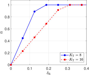
(a) Centralized Setting

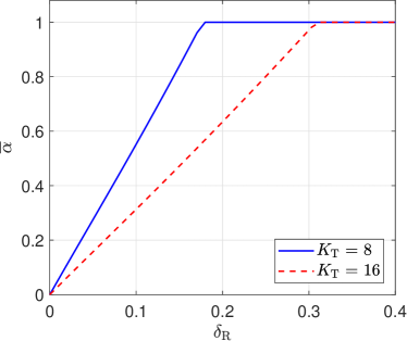
(b) Decentralized Setting

Figure 1: Tradeoff between $\delta_{\mathrm{R}}$ and $\bar{\alpha}$ for networks with $K_{\mathrm{R}}=16$, $K_{\mathrm{T}}\in\{8,16\}$, $\mu_{\mathrm{R}}={1}/{16}$ and $\mu_{\mathrm{T}}={1}/{2}$.

In this part, we investigate the implications of Theorem 1 and Theorem 2 by considering the tradeoff between the receiver cache memory size and the CSIT budget. For this purpose, we start by assuming that CSIT is perfectly available across all signalling dimensions, captured by $\alpha=1$ (equivalently $\bar{\alpha}=0$). For given $\mu_{\mathrm{T}}$ and $\mu_{\mathrm{R}}$, an achievable delivery time under centralized placement, denoted by $H_{\mathrm{C}}(\mu_{\mathrm{T}},\mu_{\mathrm{R}},1)$, is easily derived from the one-shot linear DoF in Theorem 1. Now suppose that the CSIT budget is reduced, e.g. by providing feedback for a fraction of sub-carriers. This yields $H_{\mathrm{C}}(\mu_{\mathrm{T}},\mu_{\mathrm{R}},1-\bar{\alpha})\geq H_{\mathrm{C}}(\mu_{\mathrm{T}},\mu_{\mathrm{R}},1)$, where $\bar{\alpha}$ is interpreted as the reduction in CSIT budget. We are interested in the corresponding increase in receiver cache size, i.e. $\delta_{\mathrm{R}}\in[0,1-\mu_{\mathrm{R}}]$, such that $H_{\mathrm{C}}(\mu_{\mathrm{T}},\mu_{\mathrm{R}}+\delta_{\mathrm{R}},1-\bar{\alpha})=H_{\mathrm{C}}(\mu_{\mathrm{T}},\mu_{\mathrm{R}},1)$. Note that a similar tradeoff is defined for the decentralized case through $H_{\mathrm{D}}(\mu_{\mathrm{T}},\mu_{\mathrm{R}}+\delta_{\mathrm{R}},1-\bar{\alpha})=H_{\mathrm{D}}(\mu_{\mathrm{T}},\mu_{\mathrm{R}},1)$.

The tradeoff between $\mu_{\mathrm{R}}$ and $\bar{\alpha}$ is evaluated numerically and illustrated in Fig. 1 for both centralized and decentralized cases. In particular, we consider a network of $K_{\mathrm{R}}=16$ receivers with $\mu_{\mathrm{R}}={1}/{16}$ and $\mu_{\mathrm{T}}={1}/{2}$. The number of transmitters $K_{\mathrm{T}}$ is varied between $8$ and $16$. It can be seen that the tradeoff is sharper for $K_{\mathrm{T}}=8$ compared to $K_{\mathrm{T}}=16$ in the sense that a higher reduction in CSIT $\bar{\alpha}$ can be achieved for a smaller increase in receiver cache size given by $\delta_{\mathrm{R}}$. This is due to the fact that at most $8$ orthogonal beams can be created (through e.g. zero-forcing) in the setting with $K_{\mathrm{T}}=8$, while $K_{\mathrm{T}}=16$ allows up to $16$ orthogonal beams. This makes the latter setting more dependent on CSIT in general, hence requiring a higher increase in cache size to compensate for the same reduction in CSIT budget.

III-D Related Setups

It is worthwhile highlighting that the results in Theorem 1 and Theorem 2 can be easily applied to other related setups. In particular, the N-subchannel can be replaced by a $(K_{\mathrm{T}}+1)$-th transmitter, operating on a different frequency (e.g. a WiFi access point or femtocell), and connected to all transmitter caches through a capacitated link (captured by $\bar{\alpha}$) [45]. In this case, the ergodic fading assumptions of our original setting can be relaxed, particularly if perfect CSI is also available at the $(K_{\mathrm{T}}+1)$-th transmitter.

The results also extend to the multi-server setting of [8] with wired (noiseless) linear networks, in which the parallel subchannels correspond to scenarios where servers can reach receivers through two parallel networks, a fully connected linear interference network and a multicast networks.

IV Centralized Setting: Proof of Theorem 1

In this section, we present a proof for Theorem 1. As part of the proof, we introduce a DoF upper bound which is also used in the following section in the proof of Theorem 2.

IV-A Achievability of Theorem 1

IV-A1 Placement Phase

The placement phase is analogous to the one [16]. Interestingly, this implies that the placement phase is not required to depend on the value of $\alpha$. As in [16], each file $\mathcal{W}_{n}$, $n\in[N]$, is partitioned into $\binom{K_{\mathrm{T}}}{K_{\mathrm{T}}\mu_{\mathrm{T}}}\binom{K_{\mathrm{R}}}{K_{\mathrm{R}}\mu_{\mathrm{R}}}$ disjoint subfiles of equal size, denoted by

$$\mathcal{W}_{n}=\{\mathcal{W}_{n,\mathcal{T},\mathcal{R}}\}_{\begin{subarray}{c}\mathcal{T}\subseteq[K_{\mathrm{T}}]:|\mathcal{T}|={K_{\mathrm{T}}\mu_{\mathrm{T}}}\\ \mathcal{R}\subseteq[K_{\mathrm{R}}]:|\mathcal{R}|={K_{\mathrm{R}}\mu_{\mathrm{R}}}\end{subarray}}.$$

Note that each subfile contains $\frac{F}{\binom{K_{\mathrm{T}}}{K_{\mathrm{T}}\mu_{\mathrm{T}}}\binom{K_{\mathrm{R}}}{K_{\mathrm{R}}\mu_{\mathrm{R}}}}$ packets. Each transmitter $\text{Tx}_{i}$ stores subfiles given by $\mathcal{P}_{i}=\{\mathcal{W}_{n,\mathcal{T},\mathcal{R}}:i\in\mathcal{T}\}$, while each receiver $\text{Rx}_{j}$ stores subfiles given by $\mathcal{U}_{j}=\{\mathcal{W}_{n,\mathcal{T},\mathcal{R}}:j\in\mathcal{R}\}$. It is easy to verify that such placement strategy satisfies the memory size constraints at both transmitters and receivers, and that each receiver caches $\mu_{\mathrm{R}}F$ packets from each file.

IV-A2 Delivery Phase

During the delivery phase, each receiver $\text{Rx}_{j}$ requests for a file $\mathcal{W}_{d_{j}}$. As $\text{Rx}_{j}$ has all the subfiles $\mathcal{W}_{d_{j},\mathcal{T},\mathcal{R}}$ with $j\in\mathcal{R}$ cached in its memory, it only requires the remaining subfiles given by $\mathcal{W}_{d_{j},\mathcal{T},\mathcal{R}}$ with $j\notin\mathcal{R}$. As shown in Section II-B, each packet $\mathbf{w}_{d_{j},f}$ to be delivered is split into two subpackets, i.e. $\mathbf{w}_{d_{j},f}=\big{(}\mathbf{w}^{(\mathrm{p})}_{d_{j},f},\mathbf{w}^{(\mathrm{n})}_{d_{j},n}\big{)}$. We refer to the set of P-subpackets of $\mathcal{W}_{d_{j},\mathcal{T},\mathcal{R}}$ as the P-subfile $\mathcal{W}_{d_{j},\mathcal{T},\mathcal{R}}^{(\mathrm{p})}$, and the set of N-packets of $\mathcal{W}_{d_{j},\mathcal{T},\mathcal{R}}$ as the N-subfile $\mathcal{W}_{d_{j},\mathcal{T},\mathcal{R}}^{(\mathrm{n})}$. The P-subfiles are delivered over the P-subchannel using the linear scheme in [16]. On the other hand, the N-subfiles are delivered over the N-subchannel using the original coded-multicasting scheme in [6], with the difference that superposition of coded N-subpackets over the air is used instead of XoR operations before encoding, as the latter is infeasible due to the distributed nature of transmitters. Decoding of subpackets at the receivers is carried out after taking the appropriate linear combinations, e.g. see (11) and (12). Each $\text{Rx}_{j}$ retrieves all missing P-subfiles and N-subfile and hence the file $\mathcal{W}_{d_{j}}$ is recovered.

IV-A3 Achievable One-Shot Linear DoF

Since each user has $\mu_{\mathrm{R}}F$ packets from each file stored in its cache memory, a total of $K_{\mathrm{R}}F(1-\mu_{\mathrm{R}})$ packets are delivered during the delivery phase, split into $K_{\mathrm{R}}F(1-\mu_{\mathrm{R}})$ P-subpackets and $K_{\mathrm{R}}F(1-\mu_{\mathrm{R}})$ N-subpackets delivered over the P-subchannel and N-subchannel, respectively. In what follows, we denote ${K_{\mathrm{R}}\mu_{\mathrm{R}}}$ and ${K_{\mathrm{T}}\mu_{\mathrm{T}}}$ by $m_{\mathrm{C},\mathrm{R}}$ and $m_{\mathrm{C},\mathrm{T}}$ respectively. From [16], we know that $\min\{m_{\mathrm{C},\mathrm{T}}+m_{\mathrm{C},\mathrm{R}},K_{\mathrm{R}}\}$ P-subpackets are delivered in each P-block, and hence

$$H_{\mathrm{C}}^{(\mathrm{p})}=\frac{K_{\mathrm{R}}F(1-\mu_{\mathrm{R}})}{\min\{m_{\mathrm{C},\mathrm{T}}+m_{\mathrm{C},\mathrm{R}},K_{\mathrm{R}}\}}.$$

On the other, we know from [6] that $\min\{1+m_{\mathrm{C},\mathrm{R}},K_{\mathrm{R}}\}$ N-subpackets are delivered in each N-block. Therefore, we obtain

$$H_{\mathrm{C}}^{(\mathrm{n})}=\frac{K_{\mathrm{R}}F(1-\mu_{\mathrm{R}})}{\min\{1+m_{\mathrm{C},\mathrm{R}},K_{\mathrm{R}}\}}.$$

It follows that the delivery time in time-slot is given by $H_{\mathrm{C}}=\max\Big{\{}\frac{q}{\alpha}H_{\mathrm{C}}^{(\mathrm{p})},\frac{\bar{q}}{\bar{\alpha}}H_{\mathrm{C}}^{(\mathrm{n})}\Big{\}}$. Next, we choose the splitting ratio $q$ as follow:

$$q=\frac{\alpha\cdot\min\{m_{\mathrm{C},\mathrm{T}}+m_{\mathrm{C},\mathrm{R}},K_{\mathrm{R}}\}}{\alpha\cdot\min\{m_{\mathrm{C},\mathrm{T}}+m_{\mathrm{C},\mathrm{R}},K_{\mathrm{R}}\}+\bar{\alpha}\cdot\min\{1+m_{\mathrm{C},\mathrm{R}},K_{\mathrm{R}}\}}.$$

It can be verified that the above splitting ratio satisfies $\frac{q}{\alpha}H_{\mathrm{C}}^{(\mathrm{p})}=\frac{\bar{q}}{\bar{\alpha}}H_{\mathrm{C}}^{(\mathrm{n})}$. This value of $q$ minimizes the duration of the communication which in turn maximizes the achievable DoF. Note that $q$ increases with $\alpha$, due to the fact that a larger $\alpha$ implies that the P-subchannel occupies a larger fraction of the bandwidth, hence carrying larger portions of each packet. As one may anticipate, we obtain $q=0$ and $q=1$ at the two extremes $\alpha=0$ and $\alpha=1$, respectively. With such value of $q$ we obtain

$$H_{\mathrm{C}}=\frac{K_{\mathrm{R}}F(1-\mu_{\mathrm{R}})}{\alpha\cdot\min\{m_{\mathrm{C},\mathrm{T}}+m_{\mathrm{C},\mathrm{R}},K_{\mathrm{R}}\}+\bar{\alpha}\cdot\min\{1+m_{\mathrm{C},\mathrm{R}},K_{\mathrm{R}}\}}.$$ (21)

From (21) and the fact that a total of $K_{\mathrm{R}}F(1-\mu_{\mathrm{R}})$ packets are delivered during the delivery phase, the result in (15) directly follows. This concludes the proof of achievability.

IV-B Converse of Theorem 1

To prove order optimality, we first derive an upper bound for the one-shot linear DoF.

Lemma 1.

For the cache-aided wireless network described in Section II, the one-shot linear DoF of the network, defined in (14), is bounded above as

$$\mathsf{DoF}_{\mathrm{L}}^{*}(\mu_{\mathrm{T}},\mu_{\mathrm{R}},\alpha)\leq\alpha\cdot\min\Big{\{}\frac{K_{\mathrm{T}}\mu_{\mathrm{T}}+K_{\mathrm{R}}\mu_{\mathrm{R}}}{1-\mu_{\mathrm{R}}},K_{\mathrm{R}}\Big{\}}+\bar{\alpha}\cdot\min\Big{\{}\frac{1+K_{\mathrm{R}}\mu_{\mathrm{R}}}{1-\mu_{\mathrm{R}}},K_{\mathrm{R}}\Big{\}}.$$ (22)

The proof of Lemma 1 is relegated to Appendix A. It is easily seen that by denoting the right-hand side of (22) as $\mathsf{DoF}_{\mathrm{L},\mathrm{ub}}(\mu_{\mathrm{T}},\mu_{\mathrm{R}},\alpha)$, we have

$$\mathsf{DoF}_{\mathrm{L},\mathrm{ub}}(\mu_{\mathrm{T}},\mu_{\mathrm{R}},\alpha)=\alpha\cdot\mathsf{DoF}_{\mathrm{L},\mathrm{ub}}(\mu_{\mathrm{T}},\mu_{\mathrm{R}},1)+\bar{\alpha}\cdot\mathsf{DoF}_{\mathrm{L},\mathrm{ub}}(\mu_{\mathrm{T}},\mu_{\mathrm{R}},0).$$ (23)

The expression in (23) proofs useful when proving the order-optimality parts of Theorem 1 and Theorem 2. We now proceed to prove the order-optimality part of Theorem 1.

From [16], we know that for $\alpha=1$, we have $\mathsf{DoF}_{\mathrm{L},\mathrm{ub}}(\mu_{\mathrm{T}},\mu_{\mathrm{R}},1)/\mathsf{DoF}_{\mathrm{L},\mathrm{C}}(\mu_{\mathrm{T}},\mu_{\mathrm{R}},1)\leq 2$. We show that when $\alpha=0$, we also have $\mathsf{DoF}_{\mathrm{L},\mathrm{ub}}(\mu_{\mathrm{T}},\mu_{\mathrm{R}},0)/\mathsf{DoF}_{\mathrm{L},\mathrm{C}}(\mu_{\mathrm{T}},\mu_{\mathrm{R}},0)\leq 2$. Consider the two cases:

1. $\mu_{\mathrm{R}}\leq\frac{1}{2}$: In this case, from (22) in Lemma 1 we obtain

   $$\begin{split}\mathsf{DoF}_{\mathrm{L},\mathrm{ub}}(\mu_{\mathrm{T}},\mu_{\mathrm{R}},0)&=\min\Big{\{}\frac{1+K_{\mathrm{R}}\mu_{\mathrm{R}}}{1-\mu_{\mathrm{R}}},K_{\mathrm{R}}\Big{\}}\\ &\leq\min\Big{\{}\frac{1+K_{\mathrm{R}}\mu_{\mathrm{R}}}{1-1/2},K_{\mathrm{R}}\Big{\}}\\ &\leq 2\cdot\mathsf{DoF}_{\mathrm{L},\mathrm{C}}(\mu_{\mathrm{T}},\mu_{\mathrm{R}},0).\end{split}$$

2. $\mu_{\mathrm{R}}>\frac{1}{2}$: In this case, the achievability part implies that

   $$\begin{split}\mathsf{DoF}_{\mathrm{L},\mathrm{C}}(\mu_{\mathrm{T}},\mu_{\mathrm{R}},0)&=\min\{1+K_{\mathrm{R}}\mu_{\mathrm{R}},K_{\mathrm{R}}\}\\ &>\min\{1+K_{\mathrm{R}}/2,K_{\mathrm{R}}\}>\frac{K_{\mathrm{R}}}{2}.\end{split}$$

   Since $\mathsf{DoF}_{\mathrm{L},\mathrm{ub}}(\mu_{\mathrm{T}},\mu_{\mathrm{R}},0)\leq K_{\mathrm{R}}$, we obtain $\mathsf{DoF}_{\mathrm{L},\mathrm{ub}}(\mu_{\mathrm{T}},\mu_{\mathrm{R}},0)\leq 2\cdot\mathsf{DoF}_{\mathrm{L},\mathrm{C}}(\mu_{\mathrm{T}},\mu_{\mathrm{R}},0)$.

Now we extend the above to any $\alpha\in[0,1]$. From the two above constant factor inequalities for $\alpha=1$ and $\alpha=0$, and the decomposition of the lower bound and the upper bound in (17) and (23), we obtain

$$\begin{split}\mathsf{DoF}_{\mathrm{L},\mathrm{ub}}(\mu_{\mathrm{T}},\mu_{\mathrm{R}},\alpha)&=\alpha\cdot\mathsf{DoF}_{\mathrm{L},\mathrm{ub}}(\mu_{\mathrm{T}},\mu_{\mathrm{R}},1)+\bar{\alpha}\cdot\mathsf{DoF}_{\mathrm{L},\mathrm{ub}}(\mu_{\mathrm{T}},\mu_{\mathrm{R}},0)\\ &\leq 2\alpha\cdot\mathsf{DoF}_{\mathrm{L},\mathrm{C}}(\mu_{\mathrm{T}},\mu_{\mathrm{R}},1)+2\bar{\alpha}\cdot\mathsf{DoF}_{\mathrm{L},\mathrm{C}}(\mu_{\mathrm{T}},\mu_{\mathrm{R}},0)\\ &=2\cdot\mathsf{DoF}_{\mathrm{L},\mathrm{C}}(\mu_{\mathrm{T}},\mu_{\mathrm{R}},\alpha).\end{split}$$

This completes the proof of Theorem 1.

V Decentralized Setting: Proof of Theorem 2

In this section, we present a proof of Theorem 2 starting with the achievability and then the converse.

V-A Achievability of Theorem 2

V-A1 Placement Phase

As in the centralized setting, the placement phase does not depend on $\alpha$. Each file $\mathcal{W}_{n},n\in[N]$, is partitioned into $\binom{K_{\mathrm{T}}}{K_{\mathrm{T}}\mu_{\mathrm{T}}}$ disjoint subfiles of equal size, denoted by $\mathcal{W}_{n}=\{\mathcal{W}_{n,\mathcal{T}}\}_{\begin{subarray}{c}\mathcal{T}\subseteq[K_{\mathrm{T}}]:|\mathcal{T}|={K_{\mathrm{T}}\mu_{\mathrm{T}}}\end{subarray}}$, where each subfile contains $\frac{F}{\binom{K_{\mathrm{T}}}{K_{\mathrm{T}}\mu_{\mathrm{T}}}}$ packets. Each transmitter $\text{Tx}_{i}$ then stores subfile given by $\mathcal{P}_{i}=\{\mathcal{W}_{n,\mathcal{T}}:i\in\mathcal{T}\}$. On the other end, placement at the receivers is done in a decentralized manner similar to [7]. In particular, each receiver $\text{Rx}_{i}$ stores $\mu_{\mathrm{R}}F$ packets from each file, chosen uniformly at random. Therefore, each packet of each file is stored in some subset of users $\tilde{\mathcal{R}}\subseteq[K_{\mathrm{R}}]$, where $|\tilde{\mathcal{R}}|\in\{0,1,\dots,K_{\mathrm{R}}\}$. For any $n\in[N]$, we use $\mathcal{W}_{n,\mathcal{T},\tilde{\mathcal{R}}}$ to denote the packets of file $\mathcal{W}_{n}$ which are stored by transmitters in $\mathcal{T}$ and receivers in $\tilde{\mathcal{R}}$, where $\mathcal{W}_{n,\mathcal{T},\tilde{\mathcal{R}}}$ is referred to as a mini-subfile henceforth. It follows that $\mathcal{W}_{n}$ can be reconstructed from $\big{\{}\mathcal{W}_{n,\mathcal{T},\tilde{\mathcal{R}}}:\mathcal{T}\subseteq[K_{\mathrm{T}}],|\mathcal{T}|=K_{\mathrm{T}}\mu_{\mathrm{T}},\tilde{\mathcal{R}}\subseteq[K_{\mathrm{R}}]\big{\}}$.

V-A2 Delivery Phase

Each receiver $\text{Rx}_{j}$ requests for a file $\mathcal{W}_{d_{j}}$, hence the transmitters have to deliver all mini-subfiles $\mathcal{W}_{d_{j},\mathcal{T},\tilde{\mathcal{R}}}$ with $j\notin\tilde{\mathcal{R}}$. Each packet to be delivered is split as in the centralized case, and we use $\mathcal{W}_{d_{j},\mathcal{T}}^{(\mathrm{p})}$ (P-subfile) and $\mathcal{W}_{d_{j},\mathcal{T}}^{(\mathrm{n})}$ (N-subfile) to denote the sets of P-subpackets and N-subpackets of $\mathcal{W}_{d_{j},\mathcal{T}}$, respectively. Similarly, we use $\mathcal{W}_{d_{j},\mathcal{T},\tilde{\mathcal{R}}}^{(\mathrm{p})}$ (P-mini-subfile) and $\mathcal{W}_{d_{j},\mathcal{T},\tilde{\mathcal{R}}}^{(\mathrm{n})}$ (N-mini-subfile) to denote the sets of P-subpackets and N-subpackets of $\mathcal{W}_{d_{j},\mathcal{T},\tilde{\mathcal{R}}}$, respectively.

The P-mini-subfiles are delivered over the P-subchannel, where the delivery takes place over $K_{\mathrm{R}}$ sub-phases indexed by $l\in\{0,1,\dots,K_{\mathrm{R}}-1\}$. In the $l$-th sub-phase, the transmitters delivers all $\mathcal{W}_{d_{j},\mathcal{T},\tilde{\mathcal{R}}}^{(\mathrm{p})}$ with $|\tilde{\mathcal{R}}|=l$. Note that $l$ goes up to $K_{\mathrm{R}}-1$ since for $|\tilde{\mathcal{R}}|=K_{\mathrm{R}}$, the corresponding P-mini-subfiles are cached by all receivers. For each sub-phase $l$, the delivery in the P-subchannel is reminiscent of the centralized P-subchannel delivery in Section IV-A2, with the difference that $m_{\mathrm{C},\mathrm{R}}$ in the centralized setting is replaced with $l$ here (i.e. smaller multicasting gain), as this sub-phase considers subfiles which are cached by exactly $l$ users. It follows that $\min\{m_{\mathrm{C},\mathrm{T}}+l,K_{\mathrm{R}}\}$ P-subpackets are transmitted simultaneously.

On the other hand, the N-mini-subfiles are delivered over the N-subchannel using the original decentralized coded-multicasting scheme in [7], while using over the air superposition instead of XoR. Each receiver then obtains all missing mini-subfiles and recovers the demanded file.

V-A3 Achievable One-Shot Linear DoF

We start be focusing on the delivery time over the P-subchannel. Consider the $l$-th sub-phase and an arbitrary subset of users $\tilde{\mathcal{R}}$ with size $l$. For each P-subfile $\mathcal{W}_{n,\mathcal{T}}^{(\mathrm{p})}$, $n\in[N]$, stored by some subset $\mathcal{T}$ of users), the probability that any of its P-subpackets is stored by any of the users in $\tilde{\mathcal{R}}$ is given by $\mu_{\mathrm{R}}$, as each such user caches $\mu_{\mathrm{R}}F$ random P-subpackets from each file. Hence, the probability that a P-subpacket is stored by exactly the $l$ users of $\tilde{\mathcal{R}}$ is given by $\mu_{\mathrm{R}}^{l}(1-\mu_{\mathrm{R}})^{K_{\mathrm{R}}-l}$. It follows that the expected number of P-subpackets of $\mathcal{W}_{n,\mathcal{T}}^{(\mathrm{p})}$ stored by each user in $\tilde{\mathcal{R}}$ is given by $\frac{\mu_{\mathrm{R}}^{l}(1-\mu_{\mathrm{R}})^{K_{\mathrm{R}}-l}F}{\binom{K_{\mathrm{T}}}{K_{\mathrm{T}}\mu_{\mathrm{T}}}}+o(F)$ when $F\rightarrow\infty$. The term $o(F)$ is omitted henceforth. As there is a total of $\binom{K_{\mathrm{R}}}{l}$ subsets of $l$ users, there is a total of $\frac{\binom{K_{\mathrm{R}}}{l}\mu_{\mathrm{R}}^{l}(1-\mu_{\mathrm{R}})^{K_{\mathrm{R}}-l}F}{\binom{K_{\mathrm{T}}}{K_{\mathrm{T}}\mu_{\mathrm{T}}}}$ P-subpackets of $\mathcal{W}_{n,\mathcal{T}}^{(\mathrm{p})}$ which are cached by exactly $l$ users. We now proceed to calculate number of P-subpackets of $\mathcal{W}_{d_{j}}^{(\mathrm{p})}$ stored by exactly $l$ users and have to be delivered to receiver $\text{Rx}_{j}$. For each $\mathcal{T}$, receiver $\text{Rx}_{j}$ has all P-mini-subfiles $\mathcal{W}_{d_{j},\mathcal{T},\tilde{\mathcal{R}}}^{(\mathrm{p})}$, with $|\tilde{\mathcal{R}}|=l$ and $j\in\tilde{\mathcal{R}}$, cached in its memory. Hence, $\text{Rx}_{j}$ already has $\frac{\binom{K_{\mathrm{R}}-1}{l-1}\mu_{\mathrm{R}}^{l}(1-\mu_{\mathrm{R}})^{K_{\mathrm{R}}-l}F}{\binom{K_{\mathrm{T}}}{K_{\mathrm{T}}\mu_{\mathrm{T}}}}$ P-subpackets of $\mathcal{W}_{d_{j},\mathcal{T}}^{(\mathrm{p})}$ which are cached by exactly $l$ users. It follows that the number of P-subpackets of $\mathcal{W}_{d_{j},\mathcal{T}}^{(\mathrm{p})}$ unavailable at $\text{Rx}_{j}$, given by all P-mini-subfiles $\mathcal{W}_{d_{j},\mathcal{T},\tilde{\mathcal{R}}}^{(\mathrm{p})}$ with $|\tilde{\mathcal{R}}|=l$ and $j\notin\tilde{\mathcal{R}}$, is equal to $\frac{\binom{K_{\mathrm{R}}-1}{l}\mu_{\mathrm{R}}^{l}(1-\mu_{\mathrm{R}})^{K_{\mathrm{R}}-l}F}{\binom{K_{\mathrm{T}}}{K_{\mathrm{T}}\mu_{\mathrm{T}}}}$. Considering all possible P-subfiles $\mathcal{W}_{d_{j},\mathcal{T}}^{(\mathrm{p})}$ for all $\mathcal{T}$, and as there are $K_{\mathrm{R}}$ receivers in total, the total number of P-subpackets which are stored by exactly $l$ users and have to be delivered to all receivers in the $l$-th delivery sub-phase is given by

$$K_{\mathrm{R}}\binom{K_{\mathrm{R}}-1}{l}\mu_{\mathrm{R}}^{l}(1-\mu_{\mathrm{R}})^{K_{\mathrm{R}}-l}F.$$

We recall that in the $l$-th delivery sub-phase, a total of $\min\{m_{\mathrm{C},\mathrm{T}}+l,K_{\mathrm{R}}\}$ P-subpackets are delivered simultaneously over the P-subchannel. By summing over all $K_{\mathrm{R}}$ sub-phases, we obtain

$$H^{(\mathrm{p})}_{\mathrm{D}}=K_{\mathrm{R}}\sum_{l=0}^{K_{\mathrm{R}}-1}{\frac{\binom{K_{\mathrm{R}}-1}{l}\mu_{\mathrm{R}}^{l}(1-\mu_{\mathrm{R}})^{K_{\mathrm{R}}-l}F}{\min\{m_{\mathrm{C},\mathrm{T}}+l,K_{\mathrm{R}}\}}}.$$

Moving on to the N-subchannel, as the delivery of the N-mini-subfiles follows the coded-multicasting scheme of [7], it follows that

$$H_{\mathrm{D}}^{(\mathrm{n})}=K_{\mathrm{R}}\sum_{l=0}^{K_{\mathrm{R}}-1}{\frac{\binom{K_{\mathrm{R}}-1}{l}\mu_{\mathrm{R}}^{l}(1-\mu_{\mathrm{R}})^{K_{\mathrm{R}}-l}F}{1+l}}=\frac{1-\mu_{\mathrm{R}}}{\mu_{\mathrm{R}}}\left(1-(1-\mu_{\mathrm{R}})^{K_{\mathrm{R}}}\right)F.$$

From the above, it follows that the delivery time is given by $H_{\mathrm{D}}=\max\Big{\{}\frac{q}{\alpha}H^{(\mathrm{p})}_{\mathrm{D}},\frac{\bar{q}}{\bar{\alpha}}H^{(\mathrm{n})}_{\mathrm{D}}\Big{\}}$ time-slots. As for the centralized case, we choose $q$ such that $\frac{q}{\alpha}H^{(\mathrm{p})}_{\mathrm{D}}=\frac{\bar{q}}{\bar{\alpha}}H^{(\mathrm{n})}_{\mathrm{D}}$, which in turn minimizes the duration of the communication and hence maximizes the achievable DoF. Hence, we choose

$$q=\frac{\alpha\cdot\frac{1}{\sum_{l=0}^{K_{\mathrm{R}}-1}\frac{\binom{K_{\mathrm{R}}-1}{l}\mu_{\mathrm{R}}^{l}(1-\mu_{\mathrm{R}})^{K_{\mathrm{R}}-l-1}}{\min\{K_{\mathrm{R}},K_{\mathrm{T}}{\mu}_{\mathrm{T}}+l\}}}}{\alpha\cdot\frac{1}{\sum_{l=0}^{K_{\mathrm{R}}-1}\frac{\binom{K_{\mathrm{R}}-1}{l}\mu_{\mathrm{R}}^{l}(1-\mu_{\mathrm{R}})^{K_{\mathrm{R}}-l-1}}{\min\{K_{\mathrm{R}},K_{\mathrm{T}}{\mu}_{\mathrm{T}}+l\}}}+\bar{\alpha}\cdot\frac{K_{\mathrm{R}}\mu_{\mathrm{R}}}{1-(1-\mu_{\mathrm{R}})^{K_{\mathrm{R}}}}}.$$

From the above choice of $q$ and the values of $H^{(\mathrm{p})}_{\mathrm{D}}$ and $H^{(\mathrm{p})}_{\mathrm{C}}$, it follows that

$$H_{\mathrm{D}}=\frac{K_{\mathrm{R}}F(1-\mu_{\mathrm{R}})}{\alpha\cdot\frac{1}{\sum_{l=0}^{K_{\mathrm{R}}-1}\frac{\binom{K_{\mathrm{R}}-1}{l}\mu_{\mathrm{R}}^{l}(1-\mu_{\mathrm{R}})^{K_{\mathrm{R}}-l-1}}{\min\{m_{\mathrm{C},\mathrm{T}}+l,K_{\mathrm{R}}\}}}+\bar{\alpha}\frac{K_{\mathrm{R}}\mu_{\mathrm{R}}}{\ 1-(1-\mu_{\mathrm{R}})^{K_{\mathrm{R}}}}.}$$ (24)

As a total of $K_{\mathrm{R}}F(1-\mu_{\mathrm{R}})$ packets are delivered during the delivery phase, the result in (18) directly follows from (24), which concludes the proof of achievability.

V-B Converse of Theorem 2

In this part, we prove (19) through the following steps:

• The first step of the proof is to show that when $\alpha=0$, we have the constant factor

  $$\frac{\mathsf{DoF}_{\mathrm{L},\mathrm{ub}}(\mu_{\mathrm{T}},\mu_{\mathrm{R}},0)}{\mathsf{DoF}_{\mathrm{L},\mathrm{D}}(\mu_{\mathrm{T}},\mu_{\mathrm{R}},0)}\leq 3.$$ (25)

• The following step is to show that the one-shot linear DoF ratio in (25), with $\alpha=0$, is an upper bound for the ratio with $\alpha=1$, i.e.

  $$\frac{\mathsf{DoF}_{\mathrm{L},\mathrm{ub}}(\mu_{\mathrm{T}},\mu_{\mathrm{R}},1)}{\mathsf{DoF}_{\mathrm{L},\mathrm{D}}(\mu_{\mathrm{T}},\mu_{\mathrm{R}},1)}\leq\frac{\mathsf{DoF}_{\mathrm{L},\mathrm{ub}}(\mu_{\mathrm{T}},\mu_{\mathrm{R}},0)}{\mathsf{DoF}_{\mathrm{L},\mathrm{D}}(\mu_{\mathrm{T}},\mu_{\mathrm{R}},0)}.$$ (26)

• Equipped with (25) and (26), we proceed ad follows:

  $$\begin{split}\mathsf{DoF}_{\mathrm{L},\mathrm{ub}}(\mu_{\mathrm{T}},\mu_{\mathrm{R}},\alpha)&=\alpha\cdot\mathsf{DoF}_{\mathrm{L},\mathrm{ub}}(\mu_{\mathrm{T}},\mu_{\mathrm{R}},1)+\bar{\alpha}\cdot\mathsf{DoF}_{\mathrm{L},\mathrm{ub}}(\mu_{\mathrm{T}},\mu_{\mathrm{R}},0)\\ &\leq 3\alpha\cdot\mathsf{DoF}_{\mathrm{L},\mathrm{D}}(\mu_{\mathrm{T}},\mu_{\mathrm{R}},1)+3\bar{\alpha}\cdot\mathsf{DoF}_{\mathrm{L},\mathrm{D}}(\mu_{\mathrm{T}},\mu_{\mathrm{R}},0)\\ &=3\cdot\mathsf{DoF}_{\mathrm{L},\mathrm{D}}(\mu_{\mathrm{T}},\mu_{\mathrm{R}},\alpha).\end{split}$$

It can be seen that the last of the three above steps concludes the proof of Theorem 2. Therefore, the remainder of this part is dedicated to proving the inequalities in (25) and (26).

V-B1 Proof of (25)

First, we recall that $\mathsf{DoF}_{\mathrm{L},\mathrm{D}}(\mu_{\mathrm{T}},\mu_{\mathrm{R}},0)=\frac{K_{\mathrm{R}}\mu_{\mathrm{R}}}{1-(1-\mu_{\mathrm{R}})^{K_{\mathrm{R}}}}$. Combining this with $(1-\mu_{\mathrm{R}})^{K_{\mathrm{R}}}\geq 0$ and the Bernoulli inequality $(1-\mu_{\mathrm{R}})^{K_{\mathrm{R}}}\geq 1-K_{\mathrm{R}}\mu_{\mathrm{R}}$, we obtain

$$\mathsf{DoF}_{\mathrm{L},\mathrm{D}}(\mu_{\mathrm{T}},\mu_{\mathrm{R}},0)\geq\max\Big{\{}K_{\mathrm{R}}\mu_{\mathrm{R}},1\Big{\}}.$$ (27)

For the trivial case of $K_{\mathrm{R}}=1$, it is easy to see that $\mathsf{DoF}_{\mathrm{L},\mathrm{D}}(\mu_{\mathrm{T}},\mu_{\mathrm{R}},0)=\mathsf{DoF}_{\mathrm{L},\mathrm{ub}}(\mu_{\mathrm{T}},\mu_{\mathrm{R}},0)=1$. For the case of $K_{\mathrm{R}}=2$, we have $\mathsf{DoF}_{\mathrm{L},\mathrm{D}}(\mu_{\mathrm{T}},\mu_{\mathrm{R}},0)\geq 1$ from (27) and $\mathsf{DoF}_{\mathrm{L},\mathrm{ub}}(\mu_{\mathrm{T}},\mu_{\mathrm{R}},0)\leq 2$ from (22) in Lemma 1. Hence for this case, (25) holds. Similarly, for the case $K_{\mathrm{R}}=3$, we have $\mathsf{DoF}_{\mathrm{L},\mathrm{D}}(\mu_{\mathrm{T}},\mu_{\mathrm{R}},0)\geq 1$ and $\mathsf{DoF}_{\mathrm{L},\mathrm{ub}}(\mu_{\mathrm{T}},\mu_{\mathrm{R}},0)\leq 3$ from which (25) also holds. Therefore, without loss of generality, we assume that $K_{\mathrm{R}}\geq 4$ henceforth. We proceed by considering the following cases:

1. $\mu_{\mathrm{R}}\leq{1}/{K_{\mathrm{R}}}$: For this case we have

   $$\begin{split}\mathsf{DoF}_{\mathrm{L},\mathrm{ub}}(\mu_{\mathrm{T}},\mu_{\mathrm{R}},0)&=\min\Big{\{}\frac{K_{\mathrm{R}}\mu_{\mathrm{R}}+1}{1-\mu_{\mathrm{R}}},K_{\mathrm{R}}\Big{\}}\\ &\leq\min\Big{\{}\frac{1+1}{1-1/K_{\mathrm{R}}},K_{\mathrm{R}}\Big{\}}\\ &\leq\min\Big{\{}\frac{8}{3},K_{\mathrm{R}}\Big{\}}\leq 3.\end{split}$$

   Combining the above with $\mathsf{DoF}_{\mathrm{L},\mathrm{D}}(\mu_{\mathrm{T}},\mu_{\mathrm{R}},0)\geq 1$, we conclude that (25) holds.

2. $\mu_{\mathrm{R}}\in(1/K_{\mathrm{R}},2/K_{\mathrm{R}}]$: For this case, we start by defining the function

   $$f(\mu_{\mathrm{R}})=3\mu_{\mathrm{R}}+\frac{1}{K_{\mathrm{R}}\mu_{\mathrm{R}}}.$$

   The function $f(\mu_{\mathrm{R}})$ is convex in $[0,\infty)$, and hence $f(\mu_{\mathrm{R}})\leq\max\big{(}f(\frac{1}{K_{\mathrm{R}}}),f(\frac{2}{K_{\mathrm{R}}})\big{)}$ over the interval of interest $\mu_{\mathrm{R}}\in(1/K_{\mathrm{R}},2/K_{\mathrm{R}}]$. Moreover, it is easy to verify that $f(\frac{1}{K_{\mathrm{R}}})=\frac{3}{K_{\mathrm{R}}}+1\leq\frac{7}{4}$ and $f(\frac{2}{K_{\mathrm{R}}})=\frac{6}{K_{\mathrm{R}}}+\frac{1}{2}\leq 2$. Therefore, $f(\mu_{\mathrm{R}})=3\mu_{\mathrm{R}}+\frac{1}{K_{\mathrm{R}}\mu_{\mathrm{R}}}\leq 2$ for all $K_{\mathrm{R}}$ and $\mu_{\mathrm{R}}$ of interest. Combining this with (27) and (22), we obtain

   $$\begin{split}\frac{\mathsf{DoF}_{\mathrm{L},\mathrm{ub}}(\mu_{\mathrm{T}},\mu_{\mathrm{R}},0)}{\mathsf{DoF}_{\mathrm{L},\mathrm{D}}(\mu_{\mathrm{T}},\mu_{\mathrm{R}},0)}&\leq\min\Big{\{}\frac{K_{\mathrm{R}}\mu_{\mathrm{R}}+1}{1-\mu_{\mathrm{R}}},K_{\mathrm{R}}\Big{\}}\cdot\frac{1}{\max\{K_{\mathrm{R}}\mu_{\mathrm{R}},1\}}\\ &\leq\Big{(}1+\frac{1}{K_{\mathrm{R}}\mu_{\mathrm{R}}}\Big{)}\cdot\frac{1}{1-\mu_{\mathrm{R}}}\leq 3\end{split}$$

   where the last inequality is equivalent to $3\mu_{\mathrm{R}}+\frac{1}{K_{\mathrm{R}}\mu_{\mathrm{R}}}\leq 2$. Therefore, (25) holds in this case.

3. $\mu_{\mathrm{R}}\in(2/K_{\mathrm{R}},1/2]$: For this case we have

   $$\begin{split}\mathsf{DoF}_{\mathrm{L},\mathrm{ub}}(\mu_{\mathrm{T}},\mu_{\mathrm{R}},0)&=\min\Big{\{}\frac{K_{\mathrm{R}}\mu_{\mathrm{R}}+1}{1-\mu_{\mathrm{R}}},K_{\mathrm{R}}\Big{\}}\\ &\leq\min\Big{\{}\frac{K_{\mathrm{R}}\mu_{\mathrm{R}}+1}{1-1/2},K_{\mathrm{R}}\Big{\}}\\ &=\min\Big{\{}2K_{\mathrm{R}}\mu_{\mathrm{R}}+2,K_{\mathrm{R}}\Big{\}}\\ &\leq\min\Big{\{}3K_{\mathrm{R}}\mu_{\mathrm{R}},K_{\mathrm{R}}\Big{\}}.\end{split}$$

   Combining the above with $\mathsf{DoF}_{\mathrm{L},\mathrm{D}}(\mu_{\mathrm{T}},\mu_{\mathrm{R}},0)\geq K_{\mathrm{R}}\mu_{\mathrm{R}}$, it follows that (25) holds.

4. $\mu_{\mathrm{R}}>1/2$: For this last case we have $\mathsf{DoF}_{\mathrm{L},\mathrm{D}}(\mu_{\mathrm{T}},\mu_{\mathrm{R}},0)\geq\max\{K_{\mathrm{R}}\mu_{\mathrm{R}},1\}>K_{\mathrm{R}}/2$. Combining this with $\mathsf{DoF}_{\mathrm{L},\mathrm{ub}}(\mu_{\mathrm{T}},\mu_{\mathrm{R}},0)\leq K_{\mathrm{R}}$, it follows that (25) holds, hence concluding the proof.

V-B2 Proof of (26)

From (18) and (22), the inequality in (26) can be expressed as

$$\frac{\min\Big{\{}\frac{1+K_{\mathrm{R}}\mu_{\mathrm{R}}}{1-\mu_{\mathrm{R}}},K_{\mathrm{R}}\Big{\}}}{\left(\sum_{m=0}^{K_{\mathrm{R}}-1}\frac{\binom{K_{\mathrm{R}}-1}{m}\mu_{\mathrm{R}}^{m}(1-\mu_{\mathrm{R}})^{K_{\mathrm{R}}-1-m}}{1+m}\right)^{-1}}\geq\frac{\min\Big{\{}\frac{K_{\mathrm{T}}\mu_{\mathrm{T}}+K_{\mathrm{R}}\mu_{\mathrm{R}}}{1-\mu_{\mathrm{R}}},K_{\mathrm{R}}\Big{\}}}{\left(\sum_{m=0}^{K_{\mathrm{R}}-1}\frac{\binom{K_{\mathrm{R}}-1}{m}\mu_{\mathrm{R}}^{m}(1-\mu_{\mathrm{R}})^{K_{\mathrm{R}}-1-m}}{\min\{K_{\mathrm{T}}\mu_{\mathrm{T}}+m,K_{\mathrm{R}}\}}\right)^{-1}}.$$ (28)

Defining the function $J(r)$ as

$$J(r)=\frac{\min\Big{\{}\frac{r+K_{\mathrm{R}}\mu_{\mathrm{R}}}{1-\mu_{\mathrm{R}}},K_{\mathrm{R}}\Big{\}}}{\left(\sum_{m=0}^{K_{\mathrm{R}}-1}\frac{\binom{K_{\mathrm{R}}-1}{m}\mu_{\mathrm{R}}^{m}(1-\mu_{\mathrm{R}})^{K_{\mathrm{R}}-1-m}}{\min\{r+m,K_{\mathrm{R}}\}}\right)^{-1}}$$ (29)

it can be seen that (28) is equivalent to $J(1)\geq J(K_{\mathrm{T}}\mu_{\mathrm{T}})$. In the following, we show that that $J(1)\geq J(r)$ for all $r\geq 1$. As a consequence, $J(1)\geq J(r)$ will also hold for integer values of $r$, hence for any $K_{\mathrm{T}}\mu_{\mathrm{T}}$ which is assumed to be integer for the decentralized setting and hence in Theorem 2 and in (28).

It is readily seen that for $r\geq K_{\mathrm{R}}(1-2\mu_{\mathrm{R}})$, the numerator in (29) becomes $K_{\mathrm{R}}$, and the function $J(r)$ decrease with $r$. Therefore, without loss of generality, we only consider the interval $r\in[1,K_{\mathrm{R}}(1-2\mu_{\mathrm{R}})]$ in what follows. Equivalently, for any $K_{\mathrm{R}}$ and $r$, we consider values of $\mu_{\mathrm{R}}$ that satisfy $\mu_{\mathrm{R}}\leq\frac{1}{2}\left(1-\frac{r}{K_{\mathrm{R}}}\right)$.

Next, the inequality in (28) is equivalently rewritten as

$$\frac{1+K_{\mathrm{R}}\mu_{\mathrm{R}}}{1-\mu_{\mathrm{R}}}\sum_{m=0}^{K_{\mathrm{R}}-1}{\binom{K_{\mathrm{R}}-1}{m}}\frac{\mu_{\mathrm{R}}^{m}(1-\mu_{\mathrm{R}})^{K_{\mathrm{R}}-1-m}}{1+m}\geq\frac{r+K_{\mathrm{R}}\mu_{\mathrm{R}}}{1-\mu_{\mathrm{R}}}\sum_{m=0}^{K_{\mathrm{R}}-1}{\binom{K_{\mathrm{R}}-1}{m}}\frac{\mu_{\mathrm{R}}^{m}(1-\mu_{\mathrm{R}})^{K_{\mathrm{R}}-1-m}}{\min\{r+m,K_{\mathrm{R}}\}}.$$

After rearranging the terms and removing redundant factors, the above is expressed as

$$\sum_{m=0}^{K_{\mathrm{R}}-1}\frac{{1+K_{\mathrm{R}}\mu_{\mathrm{R}}}}{1+m}{\binom{K_{\mathrm{R}}-1}{m}}\left(\frac{\mu_{\mathrm{R}}}{1-\mu_{\mathrm{R}}}\right)^{m}\geq\sum_{m=0}^{K_{\mathrm{R}}-1}\frac{{r+K_{\mathrm{R}}\mu_{\mathrm{R}}}}{\min\{r+m,K_{\mathrm{R}}\}}{\binom{K_{\mathrm{R}}-1}{m}}\left(\frac{\mu_{\mathrm{R}}}{1-\mu_{\mathrm{R}}}\right)^{m},$$

which is further rewritten as

$$\sum_{m=0}^{K_{\mathrm{R}}-1}\frac{\zeta(K_{\mathrm{R}}+1)+1}{1+m}{\binom{K_{\mathrm{R}}-1}{m}}\zeta^{m}\geq\sum_{m=0}^{K_{\mathrm{R}}-1}\frac{\zeta(K_{\mathrm{R}}+r)+r}{\min\{r+m,K_{\mathrm{R}}\}}{\binom{K_{\mathrm{R}}-1}{m}}\zeta^{m},$$ (30)

where $\zeta=\frac{\mu_{\mathrm{R}}}{1-\mu_{\mathrm{R}}}$, which is constrained as $\zeta\in\left[0,\frac{K_{\mathrm{R}}-r}{K_{\mathrm{R}}+r}\right]$ for given $K_{\mathrm{R}}$ and $r$. After further rearrangement of terms, the inequality in (30) is rewritten as

$$p(\zeta)\triangleq\sum_{m=0}^{K_{\mathrm{R}}}{c_{m}\cdot\zeta^{m}}\geq 0,$$ (31)

where $p(\zeta)$ is a polynomial in the variable $\zeta$ with coefficients given by

$$c_{m}=\begin{cases}0,\quad m=0\\ \frac{1-r}{K_{\mathrm{R}}},\quad m=K_{\mathrm{R}}\\ \binom{K_{\mathrm{R}}-1}{m-1}\cdot\left(\frac{K_{\mathrm{R}}+1}{m}-\frac{K_{\mathrm{R}}+r}{\min\{r+m-1,K_{\mathrm{R}}\}}\right)+\binom{K_{\mathrm{R}}-1}{m}\cdot\left(\frac{1}{m+1}-\frac{r}{\min\{r+m,K_{\mathrm{R}}\}}\right),\quad m\in[1,K_{\mathrm{R}}-1]_{\mathbb{Z}}.\\ \end{cases}$$

Note that in the above, we use $[a,b]_{\mathbb{Z}}$ to denote the set of all integers that are in the interval $[a,b]$, i.e. $[a,b]_{\mathbb{Z}}\triangleq[a,b]\cap\mathbb{Z}$. At this point, it is clear that the problem reduces to showing that $p(\zeta)\geq 0$ for $\zeta\in\left[0,\frac{K_{\mathrm{R}}-r}{K_{\mathrm{R}}+r}\right]$. To this end, we derive the following property of $p(\zeta)$.

Lemma 2.

The polynomial $p(\zeta)$ is quasiconcave and hence satisfies the following inequality:

$$p(\zeta)\geq\min\left(p(0),p\left(\frac{K_{\mathrm{R}}-r}{K_{\mathrm{R}}+r}\right)\right),\ \forall\zeta\in\left[0,\frac{K_{\mathrm{R}}-r}{K_{\mathrm{R}}+r}\right].$$ (32)

The proof of (32) is rather involved and hence is deferred to Appendix B. From Lemma 2, it follows that to prove that the inequality in (31) holds, it is sufficient to show that $p(0)\geq 0$ and $p\left(\frac{K_{\mathrm{R}}-r}{K_{\mathrm{R}}+r}\right)\geq 0$. Note that the case with $\zeta=0$ is trivial as $p(0)=0$. Hence, it remains to show that $p\left(\frac{K_{\mathrm{R}}-r}{K_{\mathrm{R}}+r}\right)\geq 0$ holds true. For this, we require the following inequality.

Lemma 3.

[46]. For any positive integer $K\in\mathbb{Z}_{+}$ and real number $r\in[1,K]$, we have

$$\sum_{m=1}^{K}\frac{m}{\min\{r+m-1,K\}}{\binom{K}{m}}\left(\frac{K-r}{K+r}\right)^{m}\leq\frac{K-r+2}{K+r}\left[\left(\frac{2K}{K+r}\right)^{K}-1\right].$$ (33)

The final step of the proof is to show that the inequality $p\left(\frac{K_{\mathrm{R}}-r}{K_{\mathrm{R}}+r}\right)\geq 0$ is an instance of Lemma 3, and hence holds true. Equivalently, we consider (30). By plugging $\zeta=\frac{K_{\mathrm{R}}-r}{K_{\mathrm{R}}+r}$ into (30) and multiplying both sides by $\frac{K_{\mathrm{R}}+r}{K_{\mathrm{R}}}$, the inequality $p\left(\frac{K_{\mathrm{R}}-r}{K_{\mathrm{R}}+r}\right)\geq 0$ is equivalently expressed as

$$\sum_{m=0}^{K_{\mathrm{R}}-1}\frac{K_{\mathrm{R}}-r+2}{1+m}{\binom{K_{\mathrm{R}}-1}{m}}\left(\frac{K_{\mathrm{R}}-r}{K_{\mathrm{R}}+r}\right)^{m}\geq\sum_{m=0}^{K_{\mathrm{R}}-1}\frac{K_{\mathrm{R}}+r}{\min\{r+m,K_{\mathrm{R}}\}}{\binom{K_{\mathrm{R}}-1}{m}}\left(\frac{K_{\mathrm{R}}-r}{K_{\mathrm{R}}+r}\right)^{m}.$$

By rearranging the above inequality and using the fact that $\binom{K_{\mathrm{R}}}{m+1}=\binom{K_{\mathrm{R}}-1}{m}\frac{K_{\mathrm{R}}}{m+1}$, we obtain

$$\frac{K_{\mathrm{R}}-r+2}{K_{\mathrm{R}}+r}\sum_{m=1}^{K_{\mathrm{R}}}{\binom{K_{\mathrm{R}}}{m}}\left(\frac{K_{\mathrm{R}}-r}{K_{\mathrm{R}}+r}\right)^{m}\geq\sum_{m=0}^{K_{\mathrm{R}}-1}\frac{K_{\mathrm{R}}}{\min\{r+m,K_{\mathrm{R}}\}}{\binom{K_{\mathrm{R}}-1}{m}}\left(\frac{K_{\mathrm{R}}-r}{K_{\mathrm{R}}+r}\right)^{m+1}.$$ (34)

By employing $\binom{K_{\mathrm{R}}}{m+1}=\binom{K_{\mathrm{R}}-1}{m}\frac{K_{\mathrm{R}}}{m+1}$ one more time, we finally arrive at

$$\frac{K_{\mathrm{R}}-r+2}{K_{\mathrm{R}}+r}\left[\left(\frac{2K_{\mathrm{R}}}{K_{\mathrm{R}}+r}\right)^{K_{\mathrm{R}}}-1\right]\geq\sum_{m=1}^{K_{\mathrm{R}}}\frac{m}{\min\{r+m-1,K_{\mathrm{R}}\}}{\binom{K_{\mathrm{R}}}{m}}\left(\frac{K_{\mathrm{R}}-r}{K_{\mathrm{R}}+r}\right)^{m}.$$ (35)

where in going from (34) to (35), we used the binomial identity to obtain $\sum_{m=1}^{K_{\mathrm{R}}}{\binom{K_{\mathrm{R}}}{m}}\left(\frac{K_{\mathrm{R}}-r}{K_{\mathrm{R}}+r}\right)^{m}=\left(\frac{2K_{\mathrm{R}}}{K_{\mathrm{R}}+r}\right)^{K_{\mathrm{R}}}-1$. At this point, it is evident that the inequality in (35) holds true due to (33) in Lemma 3. Therefore, (31) holds and the proof of (26) is complete.

VI Conclusions

In the paper, we considered the problem of cache-aided interference management in a wireless network where each node is equipped with a cache memory and transmission occurs over two parallel channels, one for which perfect CSIT is available and another for which no CSIT is available. Focusing on strategies with uncoded placement and separable one-shot linear delivery schemes, we characterized the optimum one-shot linear DoF to within a multiplicative factor of $2$. We further considered a decentralized setting in which content caching at the receivers is randomized. For this decentralized setting, we characterized the optimum one-shot linear DoF to within a multiplicative factor of $3$. Our results generalize and expand upon previous one-shot linear DoF results in literature, namely [8] and [16], by including the parallel no-CSIT (or multicast) channel and by considering decentralization at the receivers. The order optimality proof for the decentralized setting posed a number of technical challenges, which were circumvented by involved mathematical manipulations and employing the notion of quasiconcavity.

The results in this paper can be extended in several interesting directions. An intriguing direction would be to explore the fundamental limits of the considered setup while relaxing the restriction of uncoded placement and one-shot linear delivery schemes. While we expect uncoded placement to still be order optimal, the delivery scheme will likely rely on interference interference alignment and symbol spreading. This direction build upon and benefit from recent results reported in [17, 18, 26]. Another interesting direction would be to extend the setup and results in this paper to Fog-RAN architectures, where decentralized placement can also be afforded at the transmitters due to the supporting cloud [32, 33]. Such direction will also be relevant to D2D networks underlaying a cellular infrastructure, that performs the role of the cloud, which can benefit from the lower complexity one-shot linear schemes.

Appendix A Proof of Lemma 1

Here we present the proof of Lemma 1. We start with the observation that under average distinct demands, as opposed to worst-case demands, there is a precise characterization for the number of packets to be delivered to the receivers [16]. Since the performance under average demands is no worse than that under worst-case demands, the one-shot linear DoF in (14) is bounded above by

$$\mathsf{DoF}_{\mathrm{L}}^{*}(\mu_{\mathrm{T}},\mu_{\mathrm{R}},\alpha)\leq\frac{K_{\mathrm{R}}F(1-\mu_{\mathrm{R}})}{\overline{H}},$$ (36)

where $\overline{H}$ is a lower bound on the delivery time under average demands rather than worst-case demands. Note that the above relaxation is commonly used to obtain outer bounds in cache-aided setups, e.g. [6, 16, 20, 26]. Next, we follow the same general footsteps of [16, Sec. V] to characterize and then find a lower bound for $\overline{H}$. The steps borrowed from [16] are explained in less detail, while we elaborate more on the new challenges that arise due to packet splitting over the two subchannels.

A-A Upper bound on the Number of Subpackets Reliably Delivered Per Block

First, let us fix the caching realization $\big{(}\{\mathcal{P}_{i}\}_{i=1}^{K_{\mathrm{T}}},\{\mathcal{U}_{i}\}_{i=1}^{K_{\mathrm{R}}}\big{)}$, user demand vector $\mathbf{d}$ and splitting ratio $q$. As described in Section II-B, in each P-block or N-block, a subset of P-subpackets or N-subpacket are delivered over the P-subchannel or the N-subchannel, respectively. Let $\big{\{}\mathbf{w}_{n_{l},f_{l}}^{(\mathrm{p})}\big{\}}_{l=1}^{L^{(\mathrm{p})}}$ be a set of $L^{(\mathrm{p})}$ P-subpackets to be delivered to $L^{(\mathrm{p})}$ distinct receivers over one P-block, and $\big{\{}\mathbf{w}_{n_{l},f_{l}}^{(\mathrm{n})}\big{\}}_{l=1}^{L^{(\mathrm{n})}}$ be a set of $L^{(\mathrm{n})}$ N-subpackets to be delivered to $L^{(\mathrm{n})}$ distinct receivers over one N-block. In order for the receivers to successfully decode the transmitted subpackets, $L^{(\mathrm{p})}$ and $L^{(\mathrm{n})}$ must satisfy

$$L^{(\mathrm{p})} \leq\min_{l\in[L^{(\mathrm{p})}]}\big{\{}|\mathcal{R}_{l}|+|\mathcal{T}_{l}|\big{\}}$$ (37)

$$L^{(\mathrm{n})} \leq\min_{l\in[L^{(\mathrm{n})}]}|\mathcal{R}_{l}|+1$$ (38)

where, for any $l\in[L^{(\mathrm{p})}]$ or $l\in[L^{(\mathrm{n})}]$, $\mathcal{T}_{l}$ and $\mathcal{R}_{l}$ are the sets of transmitters and receivers, respectively, which store the packet $\mathbf{w}_{n_{l},f_{l}}=\big{(}\mathbf{w}_{n_{l},f_{l}}^{(\mathrm{p})},\mathbf{w}_{n_{l},f_{l}}^{(\mathrm{n})})$ in their caches.

The inequality in (37) follows directly from [16, Lem. 3]. On the other hand, the inequality in (38) can be shown to hold by following the same general steps used to prove [16, Lem. 3], while observing that the generic channel matrices and the lack of CSIT make the zero-forcing conditions in the proof of [16, Lem. 3] impossible to satisfy almost surely. This in turn eliminates the transmitter cooperation gain.

A-B Integer Program Formulation

For any P-block and N-block indexed by $m^{(\mathrm{p})}$ and $m^{(\mathrm{n})}$ respectively, the sets of subpackets $\mathcal{D}^{(\mathrm{p})}_{m^{(\mathrm{p})}}$ and $\mathcal{D}^{(\mathrm{n})}_{m^{(\mathrm{n})}}$ to be delivered are deemed feasible only if their cardinalities satisfy (37) and (38). Hence by keeping the caching realization, demand vector and splitting ratio fixed, the following integer programming problems yields a lower bound on the delivery time:

$${\min} \max\Big{\{}\frac{q}{\alpha}H^{(\mathrm{p})},\frac{\bar{q}}{\bar{\alpha}}H^{(\mathrm{n})}\Big{\}}$$ (39)

$$\mathrm{s.t.} \bigcup_{m^{(\mathrm{p})}=1}^{H^{(\mathrm{p})}}{\mathcal{D}^{(\mathrm{p})}_{m^{(\mathrm{p})}}}=\bigcup_{r=1}^{K_{\mathrm{R}}}{\left(\mathcal{W}^{(\mathrm{p})}_{d_{r}}\setminus\mathcal{U}_{r}^{(\mathrm{p})}\right)}$$

$$\bigcup_{m^{(\mathrm{n})}=1}^{H^{(\mathrm{n})}}{\mathcal{D}^{(\mathrm{n})}_{m^{(\mathrm{n})}}}=\bigcup_{r=1}^{K_{\mathrm{R}}}{\left(\mathcal{W}^{(\mathrm{n})}_{d_{r}}\setminus\mathcal{U}_{r}^{(\mathrm{n})}\right)}$$

$${\mathcal{D}^{(\mathrm{p})}_{m^{(\mathrm{p})}}},{\mathcal{D}^{(\mathrm{n})}_{m^{(\mathrm{n})}}}\>\>\text{are feasible},\>\>\forall m^{(\mathrm{p})}\in[H^{(\mathrm{p})}],\>\forall m^{(\mathrm{n})}\in[H^{(\mathrm{n})}].$$

The optimal value for the above problem is denoted by $H^{*\left(\{\mathcal{P}_{i}\}_{i=1}^{K_{\mathrm{T}}},\{\mathcal{U}_{i}\}_{i=1}^{K_{\mathrm{R}}},\mathbf{d},q\right)}$.

A-C From Worst-Case to Average Demands and Optimizing Over Caching Realizations and Splitting Ratios

Given a caching realization $\big{(}{\{\mathcal{P}_{i}\}_{i=1}^{K_{\mathrm{T}}},\{\mathcal{U}_{i}\}_{i=1}^{K_{\mathrm{R}}}}\big{)}$, each file $\mathcal{W}_{n}$, with $n\in[N]$, is split into $(2^{K_{\mathrm{T}}}-1)(2^{K_{\mathrm{R}}})$ subfiles $\{\mathcal{W}_{n,\mathcal{T},\mathcal{R}}\}_{\mathcal{T}\subseteq_{\emptyset}[K_{\mathrm{T}}],\mathcal{R}\subseteq[K_{\mathrm{R}}]}$, where $\mathcal{W}_{n,\mathcal{T},\mathcal{R}}$ denotes the subfile of file $\mathcal{W}_{n}$ cached by transmitters in $\mathcal{T}$ and receivers in $\mathcal{R}$, and $\mathcal{T}\subseteq_{\emptyset}[K_{\mathrm{T}}]$ denotes $\mathcal{T}\subseteq[K_{\mathrm{T}}],\mathcal{T}\neq\emptyset$. Denoting the number of packets in ${\mathcal{W}_{n,\mathcal{T},\mathcal{R}}}$ as ${a_{n,\mathcal{T},\mathcal{R}}}$, we may write an optimization problem to minimize $H^{*\left(\{\mathcal{P}_{i}\}_{i=1}^{K_{\mathrm{T}}},\{\mathcal{U}_{i}\}_{i=1}^{K_{\mathrm{R}}},\mathbf{d},q\right)}$, for the worst-case demands, over all caching realizations and splitting ratios.

As in [16], we further lower bound the delivery time by considering average demands instead of worst-case demands. In particular, by taking the average over the set of all possible $\pi(N,K_{\mathrm{R}})=\frac{N!}{(N-K_{\mathrm{R}})!}$ permutations of distinct receiver demands, denote by $\mathcal{P}_{N,K_{\mathrm{R}}}$, we write the problem:

$${\min_{\{\mathcal{P}_{i}\}_{i=1}^{K_{\mathrm{T}}},\{\mathcal{U}_{i}\}_{i=1}^{K_{\mathrm{R}}},q}}\> \frac{1}{\pi(N,K_{\mathrm{R}})}\sum_{\mathbf{d}\in\mathcal{P}_{N,K_{\mathrm{R}}}}{H^{*\left(\{\mathcal{P}_{i}\}_{i=1}^{K_{\mathrm{T}}},\{\mathcal{U}_{i}\}_{i=1}^{K_{\mathrm{R}}},\mathbf{d},q\right)}}$$ (40)

$$\mathrm{s.t.} \sum_{\begin{subarray}{c}\mathcal{T}\subseteq_{\emptyset}[K_{\mathrm{T}}]\end{subarray}}\sum_{\begin{subarray}{c}\mathcal{R}\subseteq[K_{\mathrm{R}}]\end{subarray}}{a_{n,\mathcal{T},\mathcal{R}}}=F,\>\forall n\in[N]$$

$$\sum_{n=1}^{N}\sum_{\begin{subarray}{c}\mathcal{T}\subseteq[K_{\mathrm{T}}]:\\ i\in\mathcal{T}\end{subarray}}\sum_{\begin{subarray}{c}\mathcal{R}\subseteq[K_{\mathrm{R}}]\end{subarray}}{a_{n,\mathcal{T},\mathcal{R}}}\leq\mu_{\mathrm{T}}NF,\>\forall i\in[K_{\mathrm{T}}]$$

$$\sum_{n=1}^{N}\sum_{\begin{subarray}{c}\mathcal{T}\subseteq_{\emptyset}[K_{\mathrm{T}}]\end{subarray}}\sum_{\begin{subarray}{c}\mathcal{R}\subseteq[K_{\mathrm{R}}]:\\ j\in\mathcal{R}\end{subarray}}{a_{n,\mathcal{T},\mathcal{R}}}\leq\mu_{\mathrm{R}}NF,\>\forall j\in[K_{\mathrm{R}}]$$

$$q\in[0,1],a_{n,\mathcal{T},\mathcal{R}}\geq 0,\forall n\in[N],\forall\mathcal{T}\subseteq_{\emptyset}[K_{\mathrm{T}}],\forall\mathcal{R}\subseteq[K_{\mathrm{R}}].$$

The optimum objective for the above problem is denoted by $\overline{H}$, which appears in the bound in (36). In what follows, we are interested in further lower bounding $\overline{H}$.

A-D Decoupling the P and N Subchannel and Optimizing Over Caching Realizations

To obtain a lower bound for $\bar{H}$, we consider optimizing over caching realizations for the P-subchannel and N-subchannel independently. To facilitate this, we start by observing that $H^{*\left(\{\mathcal{P}_{i}\}_{i=1}^{K_{\mathrm{T}}},\{\mathcal{U}_{i}\}_{i=1}^{K_{\mathrm{R}}},\mathbf{d},q\right)}$ in (40), the optimum objective of (39) is bounded below as

$$H^{*\left(\{\mathcal{P}_{i}\}_{i=1}^{K_{\mathrm{T}}},\{\mathcal{U}_{i}\}_{i=1}^{K_{\mathrm{R}}},\mathbf{d},q\right)}\geq\max\Big{\{}\frac{q}{\alpha}{H^{(\mathrm{p})*}}^{\left(\{\mathcal{P}_{i}\}_{i=1}^{K_{\mathrm{T}}},\{\mathcal{U}_{i}\}_{i=1}^{K_{\mathrm{R}}},\mathbf{d},q\right)},\frac{\bar{q}}{\bar{\alpha}}{H^{(\mathrm{n})*}}^{\left(\{\mathcal{P}_{i}\}_{i=1}^{K_{\mathrm{T}}},\{\mathcal{U}_{i}\}_{i=1}^{K_{\mathrm{R}}},\mathbf{d},q\right)}\Big{\}}$$ (41)

where ${H^{(\mathrm{s})*}}^{\left(\{\mathcal{P}_{i}\}_{i=1}^{K_{\mathrm{T}}},\{\mathcal{U}_{i}\}_{i=1}^{K_{\mathrm{R}}},\mathbf{d},q\right)}$, $\mathrm{s}\in\{\mathrm{p},\mathrm{n}\}$, is the optimum objective of the optimization problem

$${\min} H^{(\mathrm{s})}$$ (42)

$$\mathrm{s.t.} \bigcup_{m^{(\mathrm{s})}=1}^{H^{(\mathrm{s})}}{\mathcal{D}^{(\mathrm{s})}_{m^{(\mathrm{s})}}}=\bigcup_{r=1}^{K_{\mathrm{r}}}{\left(\mathcal{W}^{(\mathrm{s})}_{d_{r}}\setminus\mathcal{U}_{r}^{(\mathrm{s})}\right)}$$

$${\mathcal{D}^{(\mathrm{s})}_{m^{(\mathrm{s})}}}\>\>\text{is feasible},\>\>\forall m^{(\mathrm{s})}\in[H^{(\mathrm{s})}].$$

The lower bound in (41) is derived directly from problem (39), e.g. the P-subchannel term on the right-hand side of (41) is obtained by relaxing all N-subchannel components in the objective and constraints of problem (39). Denoting the average demand operator $\frac{1}{\pi(N,K_{\mathrm{R}})}\sum_{\mathbf{d}\in\mathcal{P}_{N,K_{\mathrm{R}}}}(\cdot)$ by $\operatorname{\mathbbmss{E}}_{\mathbf{d}}(\cdot)$ for brevity, it follows that the objective function of problem (40) is lower bounded as

$$\operatorname{\mathbbmss{E}}_{\mathbf{d}}\Big{(} {H^{*\left(\{\mathcal{P}_{i}\}_{i=1}^{K_{\mathrm{T}}},\{\mathcal{U}_{i}\}_{i=1}^{K_{\mathrm{R}}},\mathbf{d},q\right)}}\Big{)}\geq\operatorname{\mathbbmss{E}}_{\mathbf{d}}\Big{(}\max\Big{\{}\frac{q}{\alpha}{H^{(\mathrm{p})*}}^{\left(\{\mathcal{P}_{i}\}_{i=1}^{K_{\mathrm{T}}},\{\mathcal{U}_{i}\}_{i=1}^{K_{\mathrm{R}}},\mathbf{d},q\right)},\frac{\bar{q}}{\bar{\alpha}}{H^{(\mathrm{n})*}}^{\left(\{\mathcal{P}_{i}\}_{i=1}^{K_{\mathrm{T}}},\{\mathcal{U}_{i}\}_{i=1}^{K_{\mathrm{R}}},\mathbf{d},q\right)}\Big{\}}\Big{)}$$

$$\geq\max\Big{\{}\frac{q}{\alpha}\operatorname{\mathbbmss{E}}_{\mathbf{d}}\Big{(}{H^{(\mathrm{p})*}}^{\left(\{\mathcal{P}_{i}\}_{i=1}^{K_{\mathrm{T}}},\{\mathcal{U}_{i}\}_{i=1}^{K_{\mathrm{R}}},\mathbf{d},q\right)}\Big{)},\frac{\bar{q}}{\bar{\alpha}}\operatorname{\mathbbmss{E}}_{\mathbf{d}}\Big{(}{H^{(\mathrm{n})*}}^{\left(\{\mathcal{P}_{i}\}_{i=1}^{K_{\mathrm{T}}},\{\mathcal{U}_{i}\}_{i=1}^{K_{\mathrm{R}}},\mathbf{d},q\right)}\Big{)}\Big{\}}$$ (43)

where the inequality in (43) follows from the convexity of the pointwise maximum function and Jensen’s inequality. Next, we plug the lower bound in (43) into (40) from which we obtain a lower bound on $\overline{H}$. Moreover, for any given splitting ratio $q$, we optimize over caching realizations independently for the P-subchannel and N-subchannel through

$${\min_{\{\mathcal{P}_{i}\}_{i=1}^{K_{\mathrm{T}}},\{\mathcal{U}_{i}\}_{i=1}^{K_{\mathrm{R}}}}}\> \frac{1}{\pi(N,K_{\mathrm{R}})}\sum_{\mathbf{d}\in\mathcal{P}_{N,K_{\mathrm{R}}}}{{H^{(\mathrm{s})*}}^{\left(\{\mathcal{P}_{i}\}_{i=1}^{K_{\mathrm{T}}},\{\mathcal{U}_{i}\}_{i=1}^{K_{\mathrm{R}}},\mathbf{d},q\right)}}$$ (44)

$$\mathrm{s.t.} \sum_{\begin{subarray}{c}\mathcal{T}\subseteq_{\emptyset}[K_{\mathrm{T}}]\end{subarray}}\sum_{\begin{subarray}{c}\mathcal{R}\subseteq[K_{\mathrm{R}}]\end{subarray}}{a_{n,\mathcal{T},\mathcal{R}}}=F,\>\forall n\in[N]$$

$$\sum_{n=1}^{N}\sum_{\begin{subarray}{c}\mathcal{T}\subseteq[K_{\mathrm{T}}]:\\ i\in\mathcal{T}\end{subarray}}\sum_{\begin{subarray}{c}\mathcal{R}\subseteq[K_{\mathrm{R}}]\end{subarray}}{a_{n,\mathcal{T},\mathcal{R}}}\leq\mu_{\mathrm{T}}NF,\>\forall i\in[K_{\mathrm{T}}]$$

$$\sum_{n=1}^{N}\sum_{\begin{subarray}{c}\mathcal{T}\subseteq_{\emptyset}[K_{\mathrm{T}}]\end{subarray}}\sum_{\begin{subarray}{c}\mathcal{R}\subseteq[K_{\mathrm{R}}]:\\ j\in\mathcal{R}\end{subarray}}{a_{n,\mathcal{T},\mathcal{R}}}\leq\mu_{\mathrm{R}}NF,\>\forall j\in[K_{\mathrm{R}}]$$

$$a_{n,\mathcal{T},\mathcal{R}}\geq 0,\forall n\in[N],\forall\mathcal{T}\subseteq_{\emptyset}[K_{\mathrm{T}}],\forall\mathcal{R}\subseteq[K_{\mathrm{R}}],$$

for which we denote the optimum objective function as $\overline{H^{(\mathrm{s})}}^{\left(q\right)}$, $\mathrm{s}\in\{\mathrm{p},\mathrm{n}\}$. This yields the lower bound on $\overline{H}$ given by

$$\overline{H}\geq\min_{q\in[0,1]}\max\Big{\{}\frac{q}{\alpha}\overline{H^{(\mathrm{p})}}^{\left(q\right)},\frac{\bar{q}}{\bar{\alpha}}\overline{H^{(\mathrm{n})}}^{\left(q\right)}\Big{\}}.$$ (45)

The two components $\overline{H^{(\mathrm{p})}}^{\left(q\right)}$ and $\overline{H^{(\mathrm{n})}}^{\left(q\right)}$ can be separately lower bounded as

$$\overline{H^{(\mathrm{p})}}^{(q)} \geq\frac{K_{\mathrm{R}}F(1-\mu_{\mathrm{R}})^{2}}{{K_{\mathrm{T}}\mu_{\mathrm{T}}+K_{\mathrm{R}}\mu_{\mathrm{R}}}}$$ (46)

$$\overline{H^{(\mathrm{n})}}^{(q)} \geq\frac{K_{\mathrm{R}}F(1-\mu_{\mathrm{R}})^{2}}{{1+K_{\mathrm{R}}\mu_{\mathrm{R}}}}.$$ (47)

The lower bound in (46) follows directly from [16, Lem. 4]. On the other hand, the lower bound in (47) is derived at the end of this section by employing the same techniques in the proof of [16].

Since in the problem in (44) the total number of subpackets per block delivered over either of the two subchannels is $K_{\mathrm{R}}F\left(1-\mu_{\mathrm{R}}\right)$, and no more than $K_{\mathrm{R}}$ subpackets can be delivered simultaneously, we obtain $\overline{H^{(\mathrm{s})}}^{(q)}\geq\frac{K_{\mathrm{R}}F(1-\mu_{\mathrm{R}})}{K_{\mathrm{R}}}$. Combining this with the lower bounds in (46) and (47), we obtain

$$\overline{H^{(\mathrm{p})}}^{(q)} \geq\frac{K_{\mathrm{R}}F(1-\mu_{\mathrm{R}})}{\min\left\{\frac{K_{\mathrm{T}}\mu_{\mathrm{T}}+K_{\mathrm{R}}\mu_{\mathrm{R}}}{1-\mu_{\mathrm{R}}},K_{\mathrm{R}}\right\}}$$ (48)

$$\overline{H^{(\mathrm{n})}}^{(q)} \geq\frac{K_{\mathrm{R}}F(1-\mu_{\mathrm{R}})}{\min\left\{\frac{1+K_{\mathrm{R}}\mu_{\mathrm{R}}}{1-\mu_{\mathrm{R}}},K_{\mathrm{R}}\right\}}.$$ (49)

It is evident that the above lower bounds do not depend on the value of $q$, and by combining (48) and (49) with (45), it follows that

$$\overline{H}\geq\min_{q\in[0,1]}\max\Bigg{\{}\frac{q}{\alpha}\cdot\frac{K_{\mathrm{R}}F(1-\mu_{\mathrm{R}})}{\min\Big{\{}\frac{K_{\mathrm{T}}\mu_{\mathrm{T}}+K_{\mathrm{R}}\mu_{\mathrm{R}}}{1-\mu_{\mathrm{R}}},K_{\mathrm{R}}\Big{\}}},\frac{\bar{q}}{\bar{\alpha}}\cdot\frac{K_{\mathrm{R}}F(1-\mu_{\mathrm{R}})}{\min\Big{\{}\frac{1+K_{\mathrm{R}}\mu_{\mathrm{R}}}{1-\mu_{\mathrm{R}}},K_{\mathrm{R}}\Big{\}}}\Bigg{\}}.$$ (50)

A-E Optimizing Over Splitting Rations and Combing Bounds

The splitting ration $q$ that minimizes the right-hand side of (50), which we denote by $q^{*}$, must satisfy

$$\frac{q^{*}}{\alpha}\cdot\frac{K_{\mathrm{R}}F(1-\mu_{\mathrm{R}})}{\min\Big{\{}\frac{K_{\mathrm{T}}\mu_{\mathrm{T}}+K_{\mathrm{R}}\mu_{\mathrm{R}}}{1-\mu_{\mathrm{R}}},K_{\mathrm{R}}\Big{\}}}=\frac{\bar{q^{*}}}{\bar{\alpha}}\cdot\frac{K_{\mathrm{R}}F(1-\mu_{\mathrm{R}})}{\min\Big{\{}\frac{1+K_{\mathrm{R}}\mu_{\mathrm{R}}}{1-\mu_{\mathrm{R}}},K_{\mathrm{R}}\Big{\}}},$$

as any other $q$ leads to a larger value for the right-hand side of (50). By considering $q^{*}$, we obtain

$$\bar{H}\geq\frac{K_{\mathrm{R}}F(1-\mu_{\mathrm{R}})}{\alpha\cdot\min\Big{\{}\frac{K_{\mathrm{T}}\mu_{\mathrm{T}}+K_{\mathrm{R}}\mu_{\mathrm{R}}}{1-\mu_{\mathrm{R}}},K_{\mathrm{R}}\Big{\}}+\bar{\alpha}\cdot\min\Big{\{}\frac{1+K_{\mathrm{R}}\mu_{\mathrm{R}}}{1-\mu_{\mathrm{R}}},K_{\mathrm{R}}\Big{\}}}.$$ (51)

Combining the lower bound in (51) with the upper bound in (36), we obtain

$$\mathsf{DoF}_{\mathrm{L}}^{*}(\mu_{\mathrm{T}},\mu_{\mathrm{R}},\alpha)\leq\alpha\cdot\min\Big{\{}\frac{K_{\mathrm{T}}\mu_{\mathrm{T}}+K_{\mathrm{R}}\mu_{\mathrm{R}}}{1-\mu_{\mathrm{R}}},K_{\mathrm{R}}\Big{\}}+\bar{\alpha}\cdot\min\Big{\{}\frac{1+K_{\mathrm{R}}\mu_{\mathrm{R}}}{1-\mu_{\mathrm{R}}},K_{\mathrm{R}}\Big{\}}$$

which concludes the proof of Lemma 1.

A-F Proof of the lower bound in (47)

Note that $\overline{H^{(\mathrm{n})}}^{(q)}$ corresponds to the optimum objective value for the optimization problem in (44) when $\mathrm{s}=\mathrm{n}$. To bound this, we follow here the footsteps in the proof of [16, Lem. 4]. Starting from ${H^{(\mathrm{n})*}}^{\left(\{\mathcal{P}_{i}\}_{i=1}^{K_{\mathrm{T}}},\{\mathcal{U}_{i}\}_{i=1}^{K_{\mathrm{R}}},\mathbf{d},q\right)}$ and by invoking (38), we obtain

$${H^{(\mathrm{n})*}}^{\left(\{\mathcal{P}_{i}\}_{i=1}^{K_{\mathrm{T}}},\{\mathcal{U}_{i}\}_{i=1}^{K_{\mathrm{R}}},q,\mathbf{d}\right)}\geq\sum_{i=1}^{K_{\mathrm{T}}}\sum_{j=0}^{K_{\mathrm{R}}}\sum_{r=1}^{K_{\mathrm{R}}}\sum_{\begin{subarray}{c}\mathcal{T}\subseteq[K_{\mathrm{T}}]:\\ |\mathcal{T}|=i\end{subarray}}\sum_{\begin{subarray}{c}\mathcal{R}\subseteq[K_{\mathrm{R}}]:\\ |\mathcal{R}|=j\\ r\notin\mathcal{R}\end{subarray}}\frac{a_{d_{r},\mathcal{T},\mathcal{R}}}{j+1}.$$ (52)

By averaging over all possible demands, we obtain

$$\begin{split}\overline{H^{(\mathrm{n})}}^{\left(\{P\}_{i=1}^{\mathrm{K_{\mathrm{T}}}},\{\mathcal{U}_{i}\}_{i=1}^{\mathrm{K_{\mathcal{T}}}},q\right)}&\geq\frac{1}{\pi(N,K_{\mathrm{R}})}\sum_{i=1}^{K_{\mathrm{T}}}\sum_{j=0}^{K_{\mathrm{R}}}\sum_{r=1}^{K_{\mathrm{R}}}\sum_{\begin{subarray}{c}\mathcal{T}\subseteq[K_{\mathrm{T}}]:\\ |\mathcal{T}|=i\end{subarray}}\sum_{\begin{subarray}{c}\mathcal{R}\subseteq[K_{\mathrm{R}}]:\\ |\mathcal{R}|=j\\ r\notin\mathcal{R}\end{subarray}}{\pi(N-1,K_{\mathrm{R}}-1)}\sum_{n=1}^{N}\frac{a_{n,\mathcal{T},\mathcal{R}}}{j+1}\\ &=\frac{1}{N}\sum_{i=1}^{K_{\mathrm{T}}}\sum_{j=0}^{K_{\mathrm{R}}-1}\frac{w_{i,j}}{j+1}.\end{split}$$ (53)

where, for any $i\in[K_{\mathrm{T}}]$ and $j\in[K_{\mathrm{R}}-1]\cup{0}$, we define

$$w_{i,j}=\sum_{r=1}^{K_{\mathrm{R}}}\sum_{\begin{subarray}{c}\mathcal{T}\subseteq[K_{\mathrm{T}}]:\\ |\mathcal{T}|=i\end{subarray}}\sum_{\begin{subarray}{c}\mathcal{R}\subseteq[K_{\mathrm{R}}]:\\ |\mathcal{R}|=j\\ r\notin\mathcal{R}\end{subarray}}\sum_{n=1}^{N}{a_{n,\mathcal{T},\mathcal{R}}}=(K_{\mathrm{R}}-j)\sum_{\begin{subarray}{c}\mathcal{T}\subseteq[K_{\mathrm{T}}]:\\ |\mathcal{T}|=i\end{subarray}}\sum_{\begin{subarray}{c}\mathcal{R}\subseteq[K_{\mathrm{R}}]:\\ |\mathcal{R}|=j\end{subarray}}\sum_{n=1}^{N}{a_{n,\mathcal{T},\mathcal{R}}}.$$ (54)

It is readily seen that

$$K_{\mathrm{R}}\mu_{\mathrm{R}}NF\geq\sum_{r=1}^{K_{\mathrm{R}}}\sum_{i=1}^{K_{\mathrm{T}}}\sum_{j=0}^{K_{\mathrm{R}}}\sum_{\begin{subarray}{c}\mathcal{T}\subseteq[K_{\mathrm{T}}]:\\ |\mathcal{T}|=i\end{subarray}}\sum_{\begin{subarray}{c}\mathcal{R}\subseteq[K_{\mathrm{R}}]:\\ |\mathcal{R}|=j\\ r\in\mathcal{R}\end{subarray}}\sum_{n=1}^{N}{a_{n,\mathcal{T},\mathcal{R}}}\geq\sum_{i=1}^{K_{\mathrm{T}}}\sum_{j=0}^{K_{\mathrm{R}}-1}\frac{j}{K_{\mathrm{R}}-j}w_{i,j}$$ (55)

and

$$NF=\sum_{i=1}^{K_{\mathrm{T}}}\sum_{j=0}^{K_{\mathrm{R}}}\sum_{\begin{subarray}{c}\mathcal{T}\subseteq[K_{\mathrm{T}}]:\\ |\mathcal{T}|=i\end{subarray}}\sum_{\begin{subarray}{c}\mathcal{R}\subseteq[K_{\mathrm{R}}]:\\ |\mathcal{R}|=j\end{subarray}}\sum_{n=1}^{N}{a_{n,\mathcal{T},\mathcal{R}}}\\ \geq\sum_{i=1}^{K_{\mathrm{T}}}\sum_{j=0}^{K_{\mathrm{R}}-1}\frac{1}{K_{\mathrm{R}}-j}w_{i,j}.$$ (56)

After applying the Cauchy-Schwarz inequality, we obtain

$$\sum_{j=0}^{K_{\mathrm{R}}-1}{w_{i,j}}\leq\sqrt{\sum_{j=0}^{K_{\mathrm{R}}-1}\frac{j+1}{K_{\mathrm{R}}-j}w_{i,j}}\cdot\sqrt{\sum_{j=0}^{K_{\mathrm{R}}-1}\frac{K_{\mathrm{R}}-j}{j+1}w_{i,j}}.$$ (57)

Applying the Cauchy-Schwarz inequality again, we obtain

$$\sum_{i=1}^{K_{\mathrm{T}}}\sum_{j=0}^{K_{\mathrm{R}}-1}{w_{i,j}}\leq\sqrt{\sum_{i=1}^{K_{\mathrm{T}}}\sum_{j=0}^{K_{\mathrm{R}}-1}\frac{j+1}{K_{\mathrm{R}}-j}w_{i,j}}\cdot\sqrt{\sum_{i=1}^{K_{\mathrm{T}}}\sum_{j=0}^{K_{\mathrm{R}}-1}\frac{K_{\mathrm{R}}-j}{j+1}w_{i,j}}.$$ (58)

Moreover, from (55) and (56) we know that

$$\sum_{i=1}^{K_{\mathrm{T}}}\sum_{j=0}^{K_{\mathrm{R}}-1}\frac{j+1}{K_{\mathrm{R}}-j}w_{i,j}\leq K_{\mathrm{R}}\mu_{\mathrm{R}}NF+NF.$$ (59)

It follows that

$$\sum_{i=1}^{K_{\mathrm{T}}}\sum_{j=0}^{K_{\mathrm{R}}-1}{w_{i,j}}\leq\sqrt{K_{\mathrm{R}}\mu_{\mathrm{R}}NF+NF}\cdot\sqrt{\sum_{i=1}^{K_{\mathrm{T}}}\sum_{j=0}^{K_{\mathrm{R}}-1}\frac{K_{\mathrm{R}}-j}{j+1}w_{i,j}}.$$ (60)

Furthermore, from [16] we know that

$$\sum_{i=1}^{K_{\mathrm{T}}}\sum_{j=0}^{K_{\mathrm{R}}-1}{w_{i,j}}\geq K_{\mathrm{R}}N(1-\mu_{\mathrm{R}})F.$$ (61)

Hence, it follows that

$$\begin{split}\overline{H^{(\mathrm{n})}}^{\left(\{\mathcal{P}_{i}\}_{i=1}^{\mathrm{K_{\mathrm{T}}}},\{\mathcal{U}_{i}\}_{i=1}^{\mathrm{K_{\mathcal{T}}}},q\right)}&\geq\frac{1}{N}\sum_{i=1}^{K_{\mathrm{T}}}\sum_{j=0}^{K_{\mathrm{R}}-1}\frac{w_{i,j}}{j+1}\geq\frac{1}{K_{\mathrm{R}}N}\sum_{i=1}^{K_{\mathrm{T}}}\sum_{j=0}^{K_{\mathrm{R}}-1}\frac{K_{\mathrm{R}}-j}{j+1}w_{i,j}\\ &\geq\frac{1}{K_{\mathrm{R}}N}\cdot\frac{1}{K_{\mathrm{R}}\mu_{\mathrm{R}}NF+NF}\left(\sum_{i=1}^{K_{\mathrm{T}}}\sum_{j=0}^{K_{\mathrm{R}}-1}{w_{i,j}}\right)^{2}\\ &\geq\frac{K_{\mathrm{R}}NF\left(1-\mu_{\mathrm{R}}\right)^{2}}{K_{\mathrm{R}}\mu_{\mathrm{R}}N+N}=\frac{K_{\mathrm{R}}F\left(1-\mu_{\mathrm{R}}\right)^{2}}{1+K_{\mathrm{R}}\mu_{\mathrm{R}}}\end{split}$$ (62)

for any caching realization $\big{(}\{\mathcal{P}_{i}\}_{i=1}^{\mathrm{K_{\mathrm{T}}}},\{\mathcal{U}_{i}\}_{i=1}^{\mathrm{K_{\mathcal{T}}}}\big{)}$, which concludes the proof.

Appendix B Proof of Lemma 2

Here we present a proof of the inequality in (32). We start with the following instrumental lemma.

Lemma 4.

Consider a polynomial $\phi(\zeta)=\sum_{m=0}^{d}{a_{m}\zeta^{m}}$ for which there exists and integer $N$ in $[-1,d]_{\mathbb{Z}}$ such that the coefficients of $\phi(\zeta)$ satisfy the following condition

$$a_{m}\geq 0,\ m<N\quad\text{and}\quad a_{m}>0,\ m=N\quad\text{and}\quad a_{m}\leq 0,\ m>N$$ (63)

where the case $N=-1$ implies $a_{0},\ldots,a_{d}\leq 0$. The polynomial $\phi(\zeta)$ is quasiconcave on $\zeta\in[0,\infty)$.

Proof.

First, we note that for the cases: $N=-1$ (i.e. when $a_{m}\leq 0$ for all $m$), $N=0$ and $N=1$, the second derivative of $\phi(\zeta)$ is a polynomial with all coefficients not greater than zero. Therefore, $\phi(\zeta)$ is concave, and hence quasiconcave, on $\zeta\in[0,\infty)$. We proceed by induction. In particular, assume that the quasiconcavity hypothesis holds for all polynomials the satisfy the condition in (63) for integer $N=n$, where $n\geq 1$. Now consider a polynomial $\phi(\zeta)$ that satisfies the condition in (63) for $N=n+1$. It is readily seen that the first derivative of $\phi(\zeta)$, denoted by $\phi^{\prime}(\zeta)$, is a polynomial which satisfies the condition in (63) for $N=n$. Hence, $\phi^{\prime}(\zeta)$ is quasiconcave by the induction hypothesis. Moreover, as $n\geq 1$, it follows from (63) that $\phi^{\prime}(0)\geq 0$. It can be verified that $\phi^{\prime}(0)\geq 0$ combined with the quasiconcavity of $\phi^{\prime}(\zeta)$ guarantee that: either $\phi^{\prime}(\zeta)$ is non-negative over $[0,\infty)$, or there exists $\zeta^{\prime}\in[0,\infty)$ such that $\phi^{\prime}(\zeta)\geq 0$ over the interval $[0,\zeta^{\prime}]$ and $\phi^{\prime}(\zeta)\leq 0$ over the interval $[\zeta^{\prime},\infty)$. It follows that $\phi(\zeta)$ is eithrer non-decreasing over $[0,\infty)$, or non-decreasing over $[0,\zeta^{\prime}]$ and non-increasing over $[\zeta^{\prime},\infty)$. In both cases, $\phi(\zeta)$ is quasiconcave. This concludes the proof of Lemma 4. ∎

Next, we show that the coefficients of the polynomial $p(\zeta)$ of interest satisfy the conditions in Lemma 4. As this shows that $p(\zeta)$ is quasiconcave, the inequality in (32) directly follows by definition. The remainder of this appendix is dedicated to showing that $p(\zeta)$ is an instance of Lemma 4.

The key step of this proof is to show that the sequence $\Big{\{}\frac{c_{m}}{\binom{K_{\mathrm{R}}-1}{m-1}}\Big{\}}_{m=1}^{K_{\mathrm{R}}-1}$ is non-increasing. Supposing that this holds true, then this sequence would satisfy the condition of Lemma 4, applied only to the indices $m\in[1,K_{\mathrm{R}}-1]_{\mathbb{Z}}$. Since the sign of $\frac{c_{m}}{\binom{K_{\mathrm{R}}-1}{m-1}}$ is preserved by $c_{m}$, then $\{c_{m}\}_{m=1}^{K_{\mathrm{R}}-1}$ also satisfies the condition of Lemma 4 over $m\in[1,K_{\mathrm{R}}-1]_{\mathbb{Z}}$. Combining this with $c_{0}=0$ and $c_{K_{\mathrm{R}}}\leq 0$, it follows that $\{c_{m}\}_{m=0}^{K_{\mathrm{R}}}$ satisfies the condition of Lemma 4, which in turn concludes the proof. Therefore, our problem reduces to showing that $\frac{c_{m}}{\binom{K_{\mathrm{R}}-1}{m-1}}$ in a non-increasing over $m\in[1,K_{\mathrm{R}}-1]_{\mathbb{Z}}$.

First, it is readily seen that $c_{m}$ can be written as

$$c_{m}=\binom{K_{\mathrm{R}}-1}{m-1}\left[\left(\frac{K_{\mathrm{R}}+1}{m}-\frac{K_{\mathrm{R}}+r}{\min\{r+m-1,K_{\mathrm{R}}\}}\right)+\frac{K_{\mathrm{R}}-m}{m}\left(\frac{1}{m+1}-\frac{r}{\min\{r+m,K_{\mathrm{R}}\}}\right)\right].$$

For briefness, we denote the coefficient $\frac{c_{m}}{\binom{K_{\mathrm{R}}-1}{m-1}}$ as $c^{\prime}_{m}$. Hence, $c^{\prime}_{m}$ is given by

$$c^{\prime}_{m}=\left(\frac{K_{\mathrm{R}}+1}{m}-\frac{K_{\mathrm{R}}+r}{\min\{r+m-1,K_{\mathrm{R}}\}}\right)+\frac{K_{\mathrm{R}}-m}{m}\left(\frac{1}{m+1}-\frac{r}{\min\{r+m,K_{\mathrm{R}}\}}\right).$$

Next, let us define the integer $\tilde{r}\in[1,K_{\mathrm{R}}-1]_{\mathbb{Z}}$ as $\tilde{r}\triangleq\lfloor r\rfloor=r-\epsilon$, where $\epsilon\in[0,1)$. Using this definition, it can be shown that $c^{\prime}_{m}$, $m\in[1,K_{\mathrm{R}}-1]_{\mathbb{Z}}$, may be expressed as:

$$c^{\prime}_{m}=\begin{cases}d_{m}\triangleq\left(\frac{K_{\mathrm{R}}+1}{m}-\frac{K_{\mathrm{R}}+r}{r+m-1}\right)+\frac{K_{\mathrm{R}}-m}{m}\left(\frac{1}{m+1}-\frac{r}{r+m}\right),\ m\in[1,K_{\mathrm{R}}-\tilde{r}-1]_{\mathbb{Z}}\\ \left(\frac{K_{\mathrm{R}}+1}{K_{\mathrm{R}}-\tilde{r}}-\frac{K_{\mathrm{R}}+\tilde{r}+\epsilon}{K_{\mathrm{R}}+\epsilon-1}\right)+\frac{\tilde{r}}{K_{\mathrm{R}}-\tilde{r}}\left(\frac{1}{K_{\mathrm{R}}-\tilde{r}+1}-\frac{\tilde{r}+\epsilon}{K_{\mathrm{R}}}\right),\ m=K_{\mathrm{R}}-\tilde{r}\\ e_{m}\triangleq\left(\frac{K_{\mathrm{R}}+1}{m}-\frac{K_{\mathrm{R}}+r}{K_{\mathrm{R}}}\right)+\frac{K_{\mathrm{R}}-m}{m}\left(\frac{1}{m+1}-\frac{r}{K_{\mathrm{R}}}\right),\ m\in[K_{\mathrm{R}}-\tilde{r}+1,K_{\mathrm{R}}-1]_{\mathbb{Z}}.\end{cases}$$

Showing that $c^{\prime}_{m}$ is non-increasing in $m$ is carried out through the two following steps:

1. We show that $d_{m}$ and $e_{m}$ are both non-increasing sequences in $m$ . This guarantees that $c^{\prime}_{m}$ is non-increasing over both the intervals $[1,K_{\mathrm{R}}-\tilde{r}-1]_{\mathbb{Z}}$ and $[K_{\mathrm{R}}-\tilde{r}+1,K_{\mathrm{R}}-1]_{\mathbb{Z}}$.

2. We show that $c^{\prime}_{K_{\mathrm{R}}-\tilde{r}}\leq d_{K_{\mathrm{R}}-\tilde{r}-1}$ and $c^{\prime}_{K_{\mathrm{R}}-\tilde{r}}\geq e_{K_{\mathrm{R}}-\tilde{r}+1}$. This guarantees that $c^{\prime}_{m}$ is non-increasing over the entire interval $[1,K_{\mathrm{R}}-1]_{\mathbb{Z}}$.

Proof of Point 1): First, let us consider $d_{m}$. This can be rewritten as:

$$d_{m}=\frac{(K_{\mathrm{R}}-m+1)(r-1)}{m(m+r-1)}+\frac{(K_{\mathrm{R}}-m)(1-r)}{(m+1)(m+r)}.$$ (64)

For $r=1$, we have $d_{m}=0$ for all $m\in[1,K_{\mathrm{R}}-1]_{\mathbb{Z}}$. Hence, we consider $r\geq 1$. From (64), and after some rearrangements, the inequality $d_{m}\geq d_{m+1}$ which we wish to prove is equivalently written as

$$\frac{K_{\mathrm{R}}-m+1}{m(m+r-1)}-\frac{K_{\mathrm{R}}-m}{(m+1)(m+r)}\geq\frac{K_{\mathrm{R}}-m}{(m+1)(m+r)}-\frac{K_{\mathrm{R}}-m-1}{(m+2)(m+r+1)}.$$ (65)

Using the following notation $A=K_{\mathrm{R}}-m$, $B=m+1$ and $C=m+r$, (65) is rewritten as

$$\frac{A+1}{(B-1)(C-1)}-\frac{A}{BC}\geq\frac{A}{BC}-\frac{A-1}{(B+1)(C+1)}.$$ (66)

After further rearranging and simplifying, (66) becomes

$$ABC+B^{2}C+BC^{2}\geq A-AB^{2}-AC^{2}.$$ (67)

Since $A\geq 1,B\geq 2$ and $C\geq 2$, (67) always holds and hence $d_{m}$ is non-increasing in $m$.

Next, we consider $e_{m}$. This can be rewritten as:

$$e_{m}=\frac{K_{\mathrm{R}}+1}{m}+\frac{K_{\mathrm{R}}}{m(m+1)}-\frac{1}{m+1}-\frac{r}{m}-1$$ (68)

From (68), it follows that $e_{m}\geq e_{m+1}$ is implied by

$$\frac{K_{\mathrm{R}}+1}{m}+\frac{K_{\mathrm{R}}}{m(m+1)}-\frac{1}{m+1}-\frac{r}{m}\geq\frac{K_{\mathrm{R}}+1}{m+1}+\frac{K_{\mathrm{R}}}{(m+1)(m+2)}-\frac{1}{m+2}-\frac{r}{m+1}.$$ (69)

After some rearrangements, the inequality in (69) becomes $(K_{\mathrm{R}}+1-r)(m+2)+2K_{\mathrm{R}}-m\geq 0$, which holds as $m\geq 1$ and $K_{\mathrm{R}}\geq r$. Hence, $e_{m}$ is a non-increasing in $m$ and this part is complete.

Proof of Point 2): In order to show that $c^{\prime}_{K_{\mathrm{R}}-\tilde{r}}\leq d_{K_{\mathrm{R}}-\tilde{r}-1}$, we only need to observe the following:

$$\begin{split}c^{\prime}_{K_{\mathrm{R}}-\tilde{r}}&=\left(\frac{K_{\mathrm{R}}+1}{K_{\mathrm{R}}-\tilde{r}}-\frac{K_{\mathrm{R}}+\tilde{r}+\epsilon}{K_{\mathrm{R}}+\epsilon-1}\right)+\frac{\tilde{r}}{K_{\mathrm{R}}-\tilde{r}}\left(\frac{1}{K_{\mathrm{R}}-\tilde{r}+1}-\frac{\tilde{r}+\epsilon}{K_{\mathrm{R}}}\right)\\ &\leq\left(\frac{K_{\mathrm{R}}+1}{K_{\mathrm{R}}-\tilde{r}}-\frac{K_{\mathrm{R}}+\tilde{r}+\epsilon}{K_{\mathrm{R}}+\epsilon-1}\right)+\frac{\tilde{r}}{K_{\mathrm{R}}-\tilde{r}}\left(\frac{1}{K_{\mathrm{R}}-\tilde{r}+1}-\frac{\tilde{r}+\epsilon}{K_{\mathrm{R}}+\epsilon}\right)\\ &=d_{K_{\mathrm{R}}-\tilde{r}}\leq d_{K_{\mathrm{R}}-\tilde{r}-1}.\end{split}$$

Next, we focus on showing that $c^{\prime}_{K_{\mathrm{R}}-\tilde{r}}\geq e_{K_{\mathrm{R}}-\tilde{r}+1}$. We observe that $c^{\prime}_{K_{\mathrm{R}}-\tilde{r}}$ can be expressed as:

$$\begin{split}c^{\prime}_{K_{\mathrm{R}}-\tilde{r}}&=\left(\frac{K_{\mathrm{R}}+1}{K_{\mathrm{R}}-\tilde{r}}-\frac{K_{\mathrm{R}}+\tilde{r}+\epsilon}{K_{\mathrm{R}}+\epsilon-1}\right)+\frac{\tilde{r}}{K_{\mathrm{R}}-\tilde{r}}\left(\frac{1}{K_{\mathrm{R}}-\tilde{r}+1}-\frac{\tilde{r}+\epsilon}{K_{\mathrm{R}}}\right)\\ &=\left(\frac{\tilde{r}+1}{K_{\mathrm{R}}-\tilde{r}}-\frac{\tilde{r}+1}{K_{\mathrm{R}}+\epsilon-1}\right)+\frac{\tilde{r}}{K_{\mathrm{R}}-\tilde{r}}\left(\frac{1}{K_{\mathrm{R}}-\tilde{r}+1}-\frac{\tilde{r}+\epsilon}{K_{\mathrm{R}}}\right).\end{split}$$ (70)

On the other hand, $e_{K_{\mathrm{R}}-\tilde{r}+1}$ is given by:

$$\begin{split}e_{K_{\mathrm{R}}-\tilde{r}+1}&=\left(\frac{K_{\mathrm{R}}+1}{K_{\mathrm{R}}-\tilde{r}+1}-\frac{K_{\mathrm{R}}+\tilde{r}+\epsilon}{K_{\mathrm{R}}}\right)+\frac{\tilde{r}-1}{K_{\mathrm{R}}-\tilde{r}+1}\left(\frac{1}{K_{\mathrm{R}}-\tilde{r}+2}-\frac{\tilde{r}+\epsilon}{K_{\mathrm{R}}}\right)\\ &=\left(\frac{\tilde{r}}{K_{\mathrm{R}}-\tilde{r}+1}-\frac{\tilde{r}+\epsilon}{K_{\mathrm{R}}}\right)+\frac{\tilde{r}-1}{K_{\mathrm{R}}-\tilde{r}+1}\left(\frac{1}{K_{\mathrm{R}}-\tilde{r}+2}-\frac{\tilde{r}+\epsilon}{K_{\mathrm{R}}}\right).\end{split}$$ (71)

By taking the difference of (70) and (71), we obtain

$$c^{\prime}_{K_{\mathrm{R}}-\tilde{r}}-e_{K_{\mathrm{R}}-\tilde{r}+1}=\frac{K_{\mathrm{R}}+1-\tilde{r}-\epsilon}{(K_{\mathrm{R}}-\tilde{r})(K_{\mathrm{R}}-\tilde{r}+1)}+\frac{(\epsilon-1)(K_{\mathrm{R}}+\tilde{r}+\epsilon)}{K_{\mathrm{R}}(K_{\mathrm{R}}+\epsilon-1)}\\ +\frac{K_{\mathrm{R}}+\tilde{r}}{(K_{\mathrm{R}}-\tilde{r})(K_{\mathrm{R}}-\tilde{r}+1)(K_{\mathrm{R}}-\tilde{r}+2)}.$$ (72)

After rearranging the terms in (72), it follows that $c^{\prime}_{K_{\mathrm{R}}-\tilde{r}}-e_{K_{\mathrm{R}}-\tilde{r}+1}\geq 0$ is implied by the inequality

$$\underbrace{K_{\mathrm{R}}(K_{\mathrm{R}}+\epsilon-1)(K_{\mathrm{R}}+1-\tilde{r}-\epsilon)(K_{\mathrm{R}}-\tilde{r}+2)}_{l_{1}(\epsilon)}+\underbrace{K_{\mathrm{R}}(K_{\mathrm{R}}+\epsilon-1)(K_{\mathrm{R}}+\tilde{r})}_{l_{2}(\epsilon)}\\ +\underbrace{(\epsilon-1)(K_{\mathrm{R}}+\epsilon+\tilde{r})(K_{\mathrm{R}}-\tilde{r})(K_{\mathrm{R}}-\tilde{r}+1)(K_{\mathrm{R}}-\tilde{r}+2)}_{l_{3}(\epsilon)}\geq 0.$$ (73)

We denote the left-hand side of (73) by $l(\epsilon)=l_{1}(\epsilon)+l_{2}(\epsilon)+l_{3}(\epsilon)$. It is readily seen that $l_{1}(\epsilon)$ and $l_{3}(\epsilon)$ are second degree polynomials in the variable $\epsilon$ (i.e. parabolas). We consider the the three functions separately in order to derive a lower bound on $l(\epsilon)$.

• $l_{1}(\epsilon)$: It can be easily verified that $l_{1}(\epsilon)$ is concave with a maximum value at $\epsilon^{*}=\frac{2-\tilde{r}}{2}$. Hence, $\epsilon^{*}\leq 0$ for $\tilde{r}\geq 2$ and $\epsilon^{*}=1/2$ for $\tilde{r}=1$. As a concave parabola is decreasing for $\epsilon\geq\epsilon^{*}$ and symmetric with respect to the maximum, it follows that for $\epsilon\in[0,1)$, we have

  $$l_{1}(\epsilon)\geq l_{1}(1)=K_{\mathrm{R}}^{2}(K_{\mathrm{R}}-\tilde{r})(K_{\mathrm{R}}-\tilde{r}+2).$$ (74)

• $l_{2}(\epsilon)$: It is readily seen that for $\epsilon\in[0,1)$, the following holds

  $$l_{2}(\epsilon)\geq l_{2}(0)=K_{\mathrm{R}}(K_{\mathrm{R}}-1)(K_{\mathrm{R}}+\tilde{r}).$$ (75)

• $l_{3}(\epsilon)$: This is a convex with a minimum value at $\epsilon^{*}=\frac{-K_{\mathrm{R}}-\tilde{r}+1}{2}<0$. Hence, for $\epsilon\in[0,1)$, we have

  $$l_{3}(\epsilon)\geq l_{3}(0)=-(K_{\mathrm{R}}+\tilde{r})(K_{\mathrm{R}}-\tilde{r})(K_{\mathrm{R}}-\tilde{r}+1)(K_{\mathrm{R}}-\tilde{r}+2).$$ (76)

By summing over the lower bounds in (74), (75) and (76), it follows that for $\epsilon\in[0,1)$, we have:

$$l(\epsilon)\geq K_{\mathrm{R}}(K_{\mathrm{R}}-1)(K_{\mathrm{R}}+\tilde{r})+(K_{\mathrm{R}}-\tilde{r})(K_{\mathrm{R}}-\tilde{r}+2)(\tilde{r}^{2}-\tilde{r}-K_{\mathrm{R}}).$$ (77)

Next, we express the right-hand side of the (77) as a function of $K_{\mathrm{R}}$:

$$g(K_{\mathrm{R}})=K_{\mathrm{R}}(K_{\mathrm{R}}-1)(K_{\mathrm{R}}+\tilde{r})+(K_{\mathrm{R}}-\tilde{r})(K_{\mathrm{R}}-\tilde{r}+2)(\tilde{r}^{2}-\tilde{r}-K_{\mathrm{R}})=aK_{\mathrm{R}}^{2}+bK_{\mathrm{R}}+c$$

where $a=\tilde{r}^{2}+2\tilde{r}-3$ and $b=-\tilde{r}(2\tilde{r}^{2}-3\tilde{r}+1)$. Finally, to show that $l(\epsilon)\geq 0$, it is sufficient to show $g(K_{\mathrm{R}})\geq 0$ for all $K_{\mathrm{R}}\geq\tilde{r}$. To this end, we observe that $g(K_{\mathrm{R}})=0$ for $\tilde{r}=1$, while $g(K_{\mathrm{R}})$ is a convex parabola with a minimum value at $\frac{\tilde{r}(\tilde{r}-1/2)}{\tilde{r}+3}\leq\tilde{r}$ for $\tilde{r}>1$. In latter case, $g(K_{\mathrm{R}})$ is increasing for $K_{\mathrm{R}}\geq\tilde{r}$. As $g(\tilde{r})\geq 0$, it follows that $g(K_{\mathrm{R}})\geq 0$ for all $K_{\mathrm{R}}\geq\tilde{r}$. This concludes the proof.

References

• [1] N. Golrezaei, A. F. Molisch, A. G. Dimakis, and G. Caire, “Femtocaching and device-to-device collaboration: A new architecture for wireless video distribution,” IEEE Commun. Magazine, vol. 51, no. 4, pp. 142–149, Apr. 2013.
• [2] E. Bastug, M. Bennis, and M. Debbah, “Living on the edge: The role of proactive caching in 5G wireless networks,” IEEE Commun. Magazine, vol. 52, no. 8, pp. 82–89, Aug. 2014.
• [3] D. Liu, B. Chen, C. Yang, and A. F. Molisch, “Caching at the wireless edge: design aspects, challenges, and future directions,” IEEE Commun. Magazine, vol. 54, no. 9, pp. 22–28, Sep. 2016.
• [4] M. A. Maddah-Ali and U. Niesen, “Coding for caching: fundamental limits and practical challenges,” IEEE Commun. Magazine, vol. 54, no. 8, pp. 23–29, Aug. 2016.
• [5] G. S. Paschos, G. Iosifidis, M. Tao, D. Towsley, and G. Caire, “The role of caching in future communication systems and networks,” arXiv:1805.11721, 2018.
• [6] M. A. Maddah-Ali and U. Niesen, “Fundamental limits of caching,” IEEE Trans. Inf. Theory, vol. 60, no. 5, pp. 2856–2867, May 2014.
• [7] M. A. Maddah-Ali and U. Niesen, “Decentralized coded caching attains order-optimal memory-rate tradeoff,” IEEE/ACM Trans. Networking, vol. 23, no. 4, pp. 1029–1040, Aug 2015.
• [8] S. P. Shariatpanahi, S. A. Motahari, and B. H. Khalaj, “Multi-server coded caching,” IEEE Trans. Inf. Theory, vol. 62, no. 12, pp. 7253–7271, Dec. 2016.
• [9] A. Ghorbel, M. Kobayashi, and S. Yang, “Content delivery in erasure broadcast channels with cache and feedback,” IEEE Trans. Inf. Theory, vol. 62, no. 11, pp. 6407–6422, Nov. 2016.
• [10] M. M. Amiri and D. Gündüz, “Cache-aided content delivery over erasure broadcast channels,” IEEE Trans. Commun., vol. 66, no. 1, pp. 370–381, Jan. 2018.
• [11] S. S. Bidokhti, M. Wigger, A. Yener, and A. E. Gamal, “State-adaptive coded caching for symmetric broadcast channels,” in Proc. Asilomar Conf. Circuits, Syst. Comput., Oct. 2017, pp. 646–650.
• [12] S. S. Bidokhti, M. Wigger, and R. Timo, “Noisy broadcast networks with receiver caching,” IEEE Trans. Inf. Theory, vol. 64, no. 11, pp. 6996–7016, Nov. 2018.
• [13] M. M. Amiri and D. Gündüz, “On the capacity region of a cache-aided gaussian broadcast channel with multi-layer messages,” arXiv:1806.09894, 2018.
• [14] M. Ji, G. Caire, and A. F. Molisch, “Fundamental limits of caching in wireless D2D networks,” IEEE Trans. Inf. Theory, vol. 62, no. 2, pp. 849–869, Feb. 2016.
• [15] M. A. Maddah-Ali and U. Niesen, “Cache-aided interference channels,” in Proc. IEEE ISIT, Jun. 2015, pp. 809–813.
• [16] N. Naderializadeh, M. A. Maddah-Ali, and A. S. Avestimehr, “Fundamental limits of cache-aided interference management,” IEEE Trans. Inf. Theory, vol. 63, no. 5, pp. 3092–3107, May 2017.
• [17] F. Xu, M. Tao, and K. Liu, “Fundamental tradeoff between storage and latency in cache-aided wireless interference networks,” IEEE Trans. Inf. Theory, vol. 63, no. 11, pp. 7464–7491, Nov. 2017.
• [18] J. Hachem, U. Niesen, and S. N. Diggavi, “Degrees of freedom of cache-aided wireless interference networks,” IEEE Trans. Inf. Theory, vol. 64, no. 7, pp. 5359–5380, Jul. 2018.
• [19] J. Zhang, F. Engelmann, and P. Elia, “Coded caching for reducing CSIT-feedback in wireless communications,” in Proc. Allerton, Sep. 2015, pp. 1099–1105.
• [20] J. Zhang and P. Elia, “Fundamental limits of cache-aided wireless BC: Interplay of coded-caching and CSIT feedback,” IEEE Trans. Inf. Theory, vol. 63, no. 5, pp. 3142–3160, May 2017.
• [21] E. Lampiris, J. Zhang, and P. Elia, “Cache-aided cooperation with no CSIT,” in Proc. IEEE ISIT, Jun. 2017, pp. 2960–2964.
• [22] E. Piovano, H. Joudeh, and B. Clerckx, “On coded caching in the overloaded MISO broadcast channel,” in Proc. IEEE ISIT, Jun. 2017, pp. 2795–2799.
• [23] Y. Cao, M. Tao, F. Xu, and K. Liu, “Fundamental storage-latency tradeoff in cache-aided MIMO interference networks,” IEEE Trans. Wireless Commun., vol. 16, no. 8, pp. 5061–5076, Aug. 2017.
• [24] K. Ngo, S. Yang, and M. Kobayashi, “Scalable content delivery with coded caching in multi-antenna fading channels,” IEEE Trans. Wireless Commun., vol. 17, no. 1, pp. 548–562, Jan 2018.
• [25] S. P. Shariatpanahi, G. Caire, and B. H. Khalaj, “Physical-layer schemes for wireless coded caching,” arXiv:1711.05969, 2017.
• [26] E. Piovano, H. Joudeh, and B. Clerckx, “Generalized degrees of freedom of the symmetric cache-aided MISO broadcast channel with partial CSIT,” IEEE Trans. Inf. Theory, doi: 10.1109/TIT.2019.2914204, 2019.
• [27] Y. Cao and M. Tao, “Treating content delivery in multi-antenna coded caching as general message sets transmission: A DoF region perspective,” arXiv:1807.01432, 2018.
• [28] A. Sengupta, R. Tandon, and O. Simeone, “Fog-aided wireless networks for content delivery: Fundamental latency tradeoffs,” IEEE Trans. Inf. Theory, vol. 63, no. 10, pp. 6650–6678, Oct. 2017.
• [29] J. Kakar, S. Gherekhloo, and A. Sezgin, “Fundamental limits on delivery time in cloud-and cache-aided heterogeneous networks,” arXiv:1706.07627, 2017.
• [30] J. Zhang and O. Simeone, “Fundamental limits of cloud and cache-aided interference management with multi-antenna base stations,” arXiv:1712.04266, 2017.
• [31] J. Zhang and O. Simeone, “Cloud-edge non-orthogonal transmission for fog networks with delayed CSI at the cloud,” arXiv:1805.10024, 2018.
• [32] A. M. Girgis, O. Ercetin, M. Nafie, and T. ElBatt, “Decentralized coded caching in wireless networks: Trade-off between storage and latency,” in Proc. IEEE ISIT, Jun. 2017, pp. 2443–2447.
• [33] F. Xu and M. Tao, “Fundamental limits of decentralized caching in fog-rans with wireless fronthaul,” arXiv:1805.03613, 2018.
• [34] J. S. P. Roig, F. Tosato, and D. Gündüz, “Storage-latency trade-off in cache-aided fog radio access networks,” arXiv:1802.01983, 2018.
• [35] R. Tandon, S. A. Jafar, S. Shamai, and H. V. Poor, “On the synergistic benefits of alternating CSIT for the MISO broadcast channel,” IEEE Trans. Inf. Theory, vol. 59, no. 7, pp. 4106–4128, Jul. 2013.
• [36] B. Rassouli, C. Hao, and B. Clerckx, “DoF analysis of the MIMO broadcast channel with alternating/hybrid CSIT,” IEEE Trans. Inf. Theory, vol. 62, no. 3, pp. 1312–1325, Mar. 2016.
• [37] S. Lashgari, R. Tandon, and S. Avestimehr, “MISO broadcast channel with hybrid CSIT: Beyond two users,” IEEE Trans. Inf. Theory, vol. 62, no. 12, pp. 7056–7077, Dec. 2016.
• [38] H. Joudeh and B. Clerckx, “On the separability of parallel MISO broadcast channels under partial CSIT: A degrees of freedom region perspective,” arXiv:1905.01283, 2019.
• [39] M. Razaviyayn, G. Lyubeznik, and Z. Luo, “On the degrees of freedom achievable through interference alignment in a MIMO interference channel,” IEEE Trans. Signal Process., vol. 60, no. 2, pp. 812–821, Feb. 2012.
• [40] N. Naderializadeh, M. A. Maddah-Ali, and A. S. Avestimehr, “Cache-aided interference management in wireless cellular networks,” in Proc. IEEE ICC, May 2017, pp. 1–7.
• [41] N. Naderializadeh, M. A. Maddah-Ali, and A. S. Avestimehr, “Cache-aided interference management in wireless cellular networks,” IEEE Trans Comm., pp. 1–1, 2019.
• [42] R. H. Etkin, D. N. C. Tse, and H. Wang, “Gaussian interference channel capacity to within one bit,” IEEE Trans. Inf. Theory, vol. 54, no. 12, pp. 5534–5562, Dec. 2008.
• [43] K. Wan, D. Tuninetti, and P. Piantanida, “On the optimality of uncoded cache placement,” in Proc. IEEE ITW, Sep. 2016, pp. 161–165.
• [44] Q. Yu, M. A. Maddah-Ali, and A. S. Avestimehr, “The exact rate-memory tradeoff for caching with uncoded prefetching,” IEEE Trans. Inf. Theory, vol. 64, no. 2, pp. 1281–1296, Feb. 2018.
• [45] J. Chen, S. Yang, A. Özgür, and A. Goldsmith, “Achieving full DoF in heterogeneous parallel broadcast channels with outdated CSIT,” IEEE Trans. Inf. Theory, vol. 62, no. 7, pp. 4154–4171, Jul. 2016.
• [46] I. Pinelis, “An inequality involving a sum of power terms,” MathOverflow, uRL:https://mathoverflow.net/q/297696 (version: 2018-04-12). [Online]. Available: https://mathoverflow.net/q/297696