A minimal tight-binding model for
the quasi-one-dimensional superconductor K₂Cr₃As₃

Abstract

We present a systematic derivation of a minimal five-band tight-binding model for the description of the electronic structure of the recently discovered quasi-one-dimensional superconductor K₂Cr₃As₃. Taking as a reference the density-functional theory (DFT) calculation, we use the outcome of a Löwdin procedure to refine a Wannier projection and fully exploit the predominant weight at the Fermi level of the states having the same symmetry of the crystal structure. Such states are described in terms of five quasi-atomic $d$ orbitals: four planar orbitals, two $d_{xy}$ and two $d_{x^{2}-y^{2}}$, and a single out-of-plane one, $d_{z^{2}}$. We show that this minimal model reproduces with great accuracy the DFT band structure in a broad energy window around the Fermi energy. Moreover, we derive an explicit simplified analytical expression of such model, which includes three nearest-neighbor hopping terms along the $z$ direction and one nearest-neighbor term within the $xy$ plane. This model captures very efficiently the energy spectrum of the system and, consequently, can be used to study transport properties, superconductivity and dynamical effects in this novel class of superconductors.

I Introduction

The study of the interplay between superconductivity and magnetism has recently brought to the discovery of superconductivity in chromium-based compounds (Chen19, ). The first example of such systems was CrAs, where the superconducting transition takes place at $T_{c}=2\,$K as a result of the suppression of the antiferromagnetic transition upon applying high pressure (Wu10, ; Wu14, ; Kotegawa14, ; Nigro18, ). This experimental finding inspired the search for superconductivity in other Cr-based materials, which led to the discovery of ambient-pressure superconductivity at 6.1 K in a Cr-based arsenide, K₂Cr₃As₃, and, subsequently, in a whole class represented by the family A₂Cr₃As₃, with A being K (Bao15, ), Rb (Tang15, ), Cs (Ztang15, ) or Na (Mu18, ). Remarkably, these Cr-based superconductors have a quasi-one-dimensional (Q1D) crystal structure that consists of [(Cr₃As₃)^2-]_∞ double-walled nanotubes in which chromium atoms form the inner wall and arsenic atoms the outer one. These nanotubes are in turn separated by columns of A⁺ ions (Bao15, ; Tang15, ; Ztang15, ).

These novel superconductors display intriguing physical properties, both in the normal  (Bao15, ; Kong15, ) and in the superconducting phase (Bao15, ; Zhi15, ; Adroja15, ; Pang15, ), which are under intense investigations especially to clarify the role played by the reduced dimensionality and by the electronic correlations  (Bao15, ). This is of course an important issue since the latter are features which considerably affect the properties of a large fraction of the unconventional superconductors discovered so far.

The crystal structure of K₂Cr₃As₃ is the hexagonal one reported in Fig. 1, with $a=9.9832$ Å and $c=4.2304$ Å. The crystal structure exhibits two planes orthogonal to the $c$ axis with slightly different stoichiometry, i.e. a plane with KCr₃As₃ and a plane with K₃Cr₃As₃ stoichiometry (Bao15, ). The resistivity of K₂Cr₃As₃ shows a linear temperature dependence in a broad temperature range, which suggests a non-Fermi-liquid normal state, possibly related to a quantum criticality and/or a realization of a Luttinger liquid (Bao15, ). This occurrence has not been confirmed by Kong et al. (Kong15, ), who rather report a $T^{3}$ dependence of the resistivity from 10 to 40 K. However, it should be noted that while this result refers to measurements performed on single crystals, those reported in Ref. Bao15, have been obtained on polycrystalline samples.

The superconductivity in K₂Cr₃As₃ shows various features pointing towards an unconventional nature. An anisotropic upper critical field is reported, with different amplitudes between the cases of field applied parallel and perpendicular to the rodlike crystals (Kong15, ). NMR measurements of the nuclear spin-lattice relaxation rate $1/T_{1}$ show a strong enhancement in the Cr nanotubes of the spin fluctuations above $T_{c}$, with the power-law temperature dependence $1/T_{1}T\sim T^{-\gamma}$ ($\gamma\simeq 0.25$) being consistent with a Tomonaga-Luttinger liquid (Zhi15, ). In addition, the absence of the Hebel-Slichter coherence peak in $1/T_{1}$ below $T_{c}$ provides further evidence that the superconducting phase is unconventional (Zhi15, ). The same kind of indication comes from muon-spin rotation measurements (Adroja15, ), which provide evidence of a possible $d$-wave superconducting pairing, as well as from measurements of the temperature dependence of the penetration depth $\Delta\lambda=\lambda(T)-\lambda(0)$ (Pang15, ). For the latter, a linear behavior is observed for $T\ll T_{c}$, instead of the exponential behavior of conventional superconductors, indicating the presence of line nodes in the superconducting gap and thus supporting the hypothesis of an unconventional nature of the superconducting phase (Pang15, ).

The unusual metallic state stimulated several studies with the aim of attaining the best description of the system. ARPES studies (Watson17, ) of single crystals reveal two Q1D Fermi surface sheets with linear dispersions, without indication of any three dimensional 3D Fermi surface, as instead predicted by Density Functional Theory (DFT) calculations (Jiang15, ). The overall bandwidth of the Cr 3$d$ bands and the Fermi velocities are comparable to DFT results, indicating that the correlated Fermi liquid picture is not appropriate for K₂Cr₃As₃. Furthermore, the spectral weight of the Q1D bands decreases near the Fermi level according to a linear power law, in an energy range of 200 meV. This result has been interpreted as an issue supporting a Tomonaga-Luttinger liquid behavior.

On the other hand, measurements and modelling of K₂Cr₃As₃ spin wave excitations show that inter-tube $J$ terms are necessary to reproduce the experimental data (Taddei17, ). Furthermore, using DFT, it has been found that in-plane structural distortions, driven by unstable optical phonon modes, play an important role to control the subtle interplay between the structural properties, the electron-phonon and the magnetic interactions (Taddei18, ). These results point out the importance of both the intra- and the inter-tube dynamics, as well as the relevance of the electron-phonon and the magnetic interactions.

From theory perspective, the electronic structure of K₂Cr₃As₃ has been examined through density functional theory calculations (Jiang15, ). In contrast with other Q1D superconductors, K₂Cr₃As₃ exhibits a relatively complex electronic structure, where the Cr-3$d$ orbitals, specifically the $d_{z^{2}}$ , $d_{xy}$ and $d_{x^{2}-y^{2}}$ ones, dominate the electronic states near the Fermi energy (Jiang15, ). Several related calculations have been also developed (XWu15, ; Zhang16, ; Zhong15, ; Zhou17, ) which establish a basis for theoretical models. In particular, it has been shown (XWu15, ), by using a three-band model built from the above mentioned $3d$ orbitals, that a triplet $p_{z}$-wave pairing driven by ferromagnetic fluctuations is the leading pairing symmetry for physically realistic parameters. This result, holding in both weak and strong coupling limits, has been confirmed in a subsequent paper where a more accurate six-band model was used (Zhang16, ). Another theoretical work focuses on the study of a twisted Hubbard tube modelling the [(Cr₃As₃)^2-]_∞ structure (Zhong15, ). Here, a three-channel effective Hamiltonian describing a Tomonaga-Luttinger liquid is derived and it is shown, within this scenario, that the system tends to exhibit triplet superconducting instabilities within a reasonable range of the interaction parameters. Finally, the superconducting phase has also been investigated by means of an extended Hubbard model with three molecular orbitals in each unit cell (Zhou17, ); as in the previously mentioned approaches, it is found that the dominant pairing channel is always a spin-triplet one, both for small and large $U$.

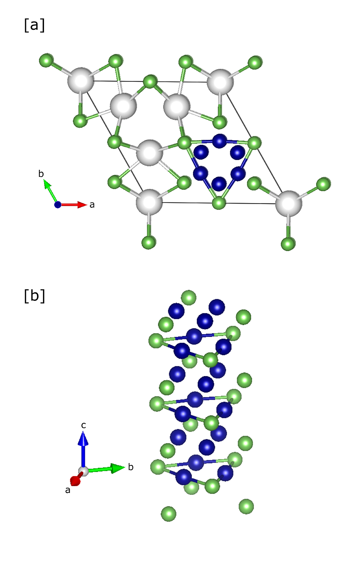
Figure 1: Crystal structure of K₂Cr₃As₃. The colours blue, green and white denote Cr, As and K atoms, respectively. (a) Top view of the primitive cell. (b) The double-walled nanotube formed by Cr and As atoms.

In this paper, we present the construction of a minimal tight-binding (TB) model hamiltonian, which reproduces with high accuracy the band structure of K₂Cr₃As₃ around the Fermi level, as obtained via first-principle calculations. We demonstrate that such description can be derived starting from a minimal set of five quasi-atomic orbitals with mainly $d$ character, namely four planar orbitals ($d_{xy}$ and $d_{x^{2}-y^{2}}$ for each of the two planes KCr₃As₃ and K₃Cr₃As₃) and a single out-of-plane one ($d_{z^{2}}$). Moreover, we derive an explicit simplified analytical expression of our five-band TB model, which includes three nearest-neighbor (NN) hopping terms along the $z$ direction and one NN within the $xy$ plane.

Such TB representation of the K₂Cr₃As₃ band structure is obtained within a three-stage approach consisting of the following steps: (i) Guided by first-principles DFT calculations, we first construct the model based on the atomic Cr and As orbitals and use it to investigate the orbital character and the symmetry of the bands which dominate in a certain energy window around the Fermi level; (ii) we use the Löwdin procedure to downfold the original full hamiltonian into a much smaller space spanned by a set of atomic Cr and As orbitals which are symmetric with respect to the basal plane; iii) the knowledge of the results of steps i) and ii) allows to formulate, within a Wannier projection, a TB description based on five atomic-like orbitals of mainly $d$ character, which are spatially localized around virtual lattice sites located at the center of the Cr-triangles of the K₃Cr₃As₃ planes, stacked along the chain direction.

We point out that this minimal model well reproduces all the details of the low-energy band structures in a broad energy region around the Fermi level, which makes it a remarkable improvement with respect to previous three-band models. Moreover, we expect that, by solving such minimal model and its extensions using suitable approximations, one may obtain information about the superconducting pairing mechanism especially for the pairing symmetry, starting from a more complete band structure.

The paper is organized as follows. In the next Section, we present the details of the DFT calculations as well as their extension taking into account the effect of the local Hubbard interaction. In Sec. III, we present the TB description in terms of atomic orbitals, which serves as a starting point for the study of the total and the local density of states, together with the characterization of the Cr and As orbital components of the electronic bands. In Sec. IV, we present the results of the Löwdin down-folding procedure giving the projection of the total Hamiltonian on the subspace of the orbitals that dominate at the Fermi level. From the results of this last section, we are able to identify the relevant orbitals at the Fermi level, so that we formulate a minimal five-band effective tight-binding model, as described in Section V, whereas last Section contains our conclusions.

II Density functional calculations

In this section, we present the first-principle calculations which supply a basis for constructing the TB modeling of the K₂Cr₃As₃ band structure that will be described in the following sections. The real space Hamiltonian matrix elements have been set according to the outcome of DFT calculations (CAutieri17, ), performed by using the VASP package (vasp, ). In such an approach, the core and the valence electrons have been treated within the projector augmented wave method (vasp1, ) and with a cutoff of 500 eV for the plane wave basis. All the calculations have been performed using a 4$\times$4$\times$10 $k$-point grid. For the treatment of the exchange correlation, the local density approximation and the Perdew-Zunger (Perdew, ) parametrization of the Ceperley-Alder (Ceperley, ) data have been considered. After obtaining the Bloch wave functions, the maximally localized Wannier functions (Marzari97, ; Souza01, ) are constructed using the WANNIER90 code (Mostofi08, ). To extract the Cr 3$d$ and As 4$p$ electronic bands, the Slater-Koster interpolation scheme has been used, in order to determine the real-space Hamiltonian matrix elements (Mostofi08, ).

The role of the electronic correlations on the energy spectrum of K₂Cr₃As₃ has also been explored. To this purpose, we have performed first-principle calculations taking into account the effect of the local Hubbard interactions, assumed to be non-vanishing on all the Cr $d$ orbitals, and efficiently parametrized by a finite number of Slater integrals. We follow the convention (Anisimov93, ) of identifying $U$ with the Slater integral $F^{0}$ and the Hund coupling with $F^{2}$ and $F^{4}$. The direct calculation gives for the intra-$t_{2g}$ orbital Hund interaction the value $J_{H}$ = 0.15 $U$ (Vaugier12, ). Considering that previous studies (Jiang15, ) indicate that the system is weakly correlated, we have assumed for $U$ values ranging in a interval going from 0 to 4 eV. The band structure obtained in the two limiting cases of $U=0$ and $U=4$ eV is reported in Fig. 2. As far as the $U=0$ case is concerned, the results are in agreement with the literature (Jiang15, ). The character of the bands at low energies is mainly due to the $d$ states of Cr atoms, whereas the $p$ states of the As atoms are located few electronvolts above and below the Fermi level, as also found for CrAs (Autieri17, ; Autieri18, ; CAutieri17, ).

We can see that, apart from a slight increase of the energy bandwidth corresponding to the chromium states being pushed away from the Fermi level, electronic correlations on chromium orbitals barely affect the energy spectrum. In particular, the band energy separation occurring when the Coulomb repulsion is turned on is one order of magnitude lower than the value of $U$ considered in the calculation. This result thus seems to confirm that K₂Cr₃As₃ is in a moderate-coupling regime, characterized by a robust metallic phase, expected to remain stable also under the influence of pressure, strain or doping. As also found for CrAs (CAutieri17, ), the nonmagnetic and the antiferromagnetic phases turn out to be very close in energy. In the case of K₂Cr₃As₃, the triangular geometry tends to frustrate antiferromagnetism, so that the nonmagnetic phase is the most stable one.

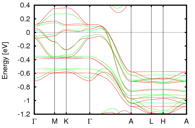
Figure 2: LDA+U band structure near the Fermi level for $U=0$ (green lines) and $U=4$ eV (red lines).

III Tight binding approximation and orbital characterization of the band structure

In this section, we derive a TB model obtained from a basis set of localized atomic orbitals at each site of the crystal structure. Our starting point will be the most reliable TB description that is capable to reproduce the LDA band structure close to the Fermi level. This description will then be used to examine in detail the orbital character of the energy bands, which will be resolved both with respect to the energy itself and to the $k$ vector in the main high-symmetry points of the Brillouin zone.

We construct the TB model by considering all the atomic orbitals that participate to conduction, namely Cr 3$d$ and As 4$p$ orbitals. The basis in the Hilbert space is given by the vector

$$\phi_{i}^{\dagger}=(d_{i,xy}^{\dagger},d_{i,x^{2}-y^{2}}^{\dagger},d_{i,z^{2}}^{\dagger},p_{i,x}^{\dagger},p_{i,y}^{\dagger},d_{i,yz}^{\dagger},d_{i,xz}^{\dagger},p_{i,z}^{\dagger}),$$ (1)

where $i$ is the lattice index and the orbitals are ordered having first those symmetric with respect to the basal plane and then the antisymmetric ones.

The tight-binding Hamiltonian is defined as

$$H=\sum_{i}\phi_{i}^{\dagger}\hat{\varepsilon}_{i}\phi_{i}+\sum_{i,j}\phi_{i}^{\dagger}\hat{t}_{i,j}\phi_{j}$$ (2)

where $i$ and $j$ denote the positions of Cr or As atoms in the crystal, and $\hat{\varepsilon}_{i}$ and $\hat{t}_{i,j}$ are matrices whose elements have indices associated with the different orbitals involved. The first term of the Hamiltonian takes into account the on-site energies, with $\left(\hat{\varepsilon}_{i}\right)^{\alpha\beta}=\varepsilon_{i}^{\alpha}\delta_{\alpha,\beta}$, while the second term describes hopping processes between distinct orbitals, with amplitudes given by the matrix elements $t_{ij}^{\alpha\beta}$. The latter are given by the expectation values of the residual lattice potential $V({\bf r})$ on the complete orthogonal set of the Wannier functions $\phi_{\alpha}({\bf r}-{\bf R}_{i})$:

$$t_{ij}^{\alpha\beta}=\bigl{\langle}\phi_{\alpha}({\bf r}-{\bf R}_{i})|V({\bf r})|\phi_{\beta}({\bf r}-{\bf R}_{j})\bigr{\rangle}\;.$$ (3)

Their values are obtained according to the procedure described in the previous Section. The Hamiltonian in Eq. (2) is a $48\times 48$ matrix because the primitive cell contains six Cr and six As atoms and we have to consider five $d$ orbitals for each Cr atom and three $p$ orbitals for each As atom.

Recently, we have carried out a detailed TB analysis in order to address the nature of the electronic bands provided by ab-initio calculations, in particular with respect to its supposed one-dimensionality (Cuono18, ). Such study revealed that considering only the hoppings between the orbitals of the atoms that lie within a single sub-nanotube fails completely to describe the in-plane band structure, not even allowing the correct description of the band structure along the $z$ axis. Such result is also in agreement with previous DFT calculations showing that, in contrast with other quasi-1D superconductors, K₂Cr₃As₃ exhibits a relatively complex electronic structure and the Fermi surface contains both 1D and 3D components (Jiang15, ).

In order to understand how the band structure is affected by the number and the position of the lattice cells involved in the hopping processes, here we have carried out a more accurate optimization of the TB hamiltonian, as explained in detail in Appendix A. Such procedure starts by first considering the hopping processes within the quasi one-dimensional [(Cr₃As₃)^2-]^∞ double-walled nanotubes only, and then including step by step inter-tube and longer-range intra-tube processes. Our analysis suggests that the LDA results arise from a delicate combination of several very small contributions, which are crucial in order to faithfully determine the dispersion of the bands that cut the Fermi level perpendicular to the chain direction ($\Gamma MK\Gamma$ path). We thus conclude that, in order to obtain a faithful representation of the electronic ab-initio band structure, it is necessary to take into account all hopping processes up to the fifth-neighbor cells along the $z$-axis, together with the in-plane hoppings up to the second-neighbor cells. Diagonalizing the Hamiltonian in Eq. 2 and retaining such hopping terms, we obtain an energy spectrum that perfectly matches the one for $U=0$ in Fig. 2 (see Fig. 16), as evaluated along the high symmetry path of the hexagonal Brillouin zone considered in Ref. Setyawan10, . Accordingly, the results presented in this section have been obtained within this framework. However, although the agreement is extremely satisfactory, we cannot consider successfully concluded our quest for a minimal model because of the need for so many hopping parameters. Therefore, in order to gain sufficient insight in the behavior of the system and design an efficient reduction procedure leading us to a real minimal model, we proceed with the analysis of the partial density of states and of the orbital character of the bands.

In order to evaluate the orbital character of the low-energy excitations around the Fermi level, we calculate the total density of states (DOS), together with its projection on the Cr and As relevant orbitals. The total DOS is obtained from the standard definition

$$\rho(\epsilon)=\frac{1}{N}\sum_{\bm{k}}\delta(\epsilon-\epsilon_{\bm{k}})$$ (4)

in which $\epsilon_{\bm{k}}$ is the energy dispersion as obtained from the tight-binding calculation presented in the previous Section, and the sum is carried out on the Brillouin zone, our grid consisting of $6\times 6\times 12$ $\bm{k}$ points. The delta functions in Eq. (4) have been approximated by Gaussian functions where the variance is assumed to be $\sigma=$ 0.025 eV. The total DOS reported in Fig. 3 exhibits, as expected, peaks in correspondence of the flat portions of the energy spectrum. Similarly to what found for CrAs (Autieri17, ; Autieri18, ; CAutieri17, ), the DOS has a predominant As character at energies of the order of $\pm 2\,$eV away from the Fermi level. The peaks near -0.5 eV and 1 eV are instead associated with the Cr-$d_{yz}$ and $d_{xz}$ orbitals, whereas, differently from what happens for CrAs, there is no clear prevalence of Cr states around the Fermi energy, but rather the Cr-$d_{xy}$, $d_{x^{2}-y^{2}}$ and $d_{z^{2}}$ and the As-$p_{x}$ and $p_{y}$ contributions are all relevant, as we will point out below in more detail.

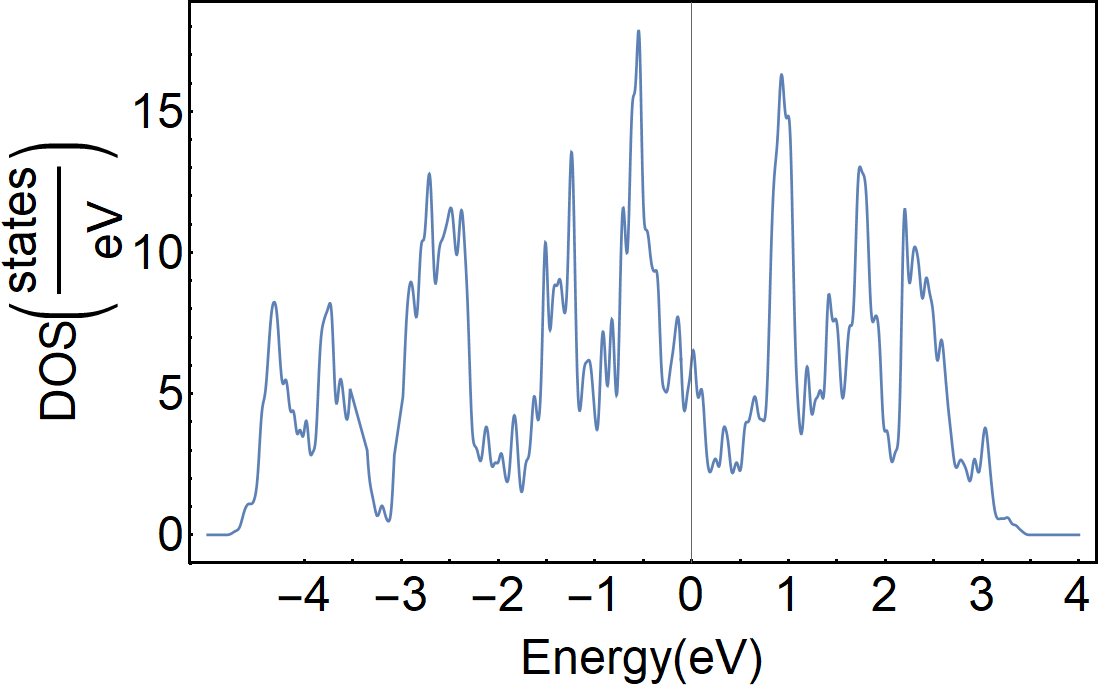
Figure 3: Total density of states of K₂Cr₃As₃ (Fermi level is at zero energy).

We have also determined the projections of the total DOS on the orbitals of the Cr or As atoms of the material. These are defined as

$$\rho_{\alpha}(\epsilon)=\frac{1}{N}\sum_{\bm{k}}|\bigl{\langle}\psi_{\bm{k}}|f_{\alpha}\bigr{\rangle}|^{2}\delta(\epsilon-\epsilon_{\bm{k}})$$ (5)

where $\psi_{\bm{k}}$ are the eigenstates of our problem and $f_{\alpha}$ represents the orbital on which we project (the delta functions are again approximated with Gaussians). The projected DOSs associated with the orbitals symmetric with respect to the basal plane, i.e. $d_{xy}$, $d_{x^{2}-y^{2}}$, $d_{z^{2}}$, $p_{x}$, $p_{y}$, are shown in Fig. 4, while those associated with the antisymmetric ones, i.e. $d_{yz}$, $d_{xz}$, $p_{z}$, are presented in Fig. 5.

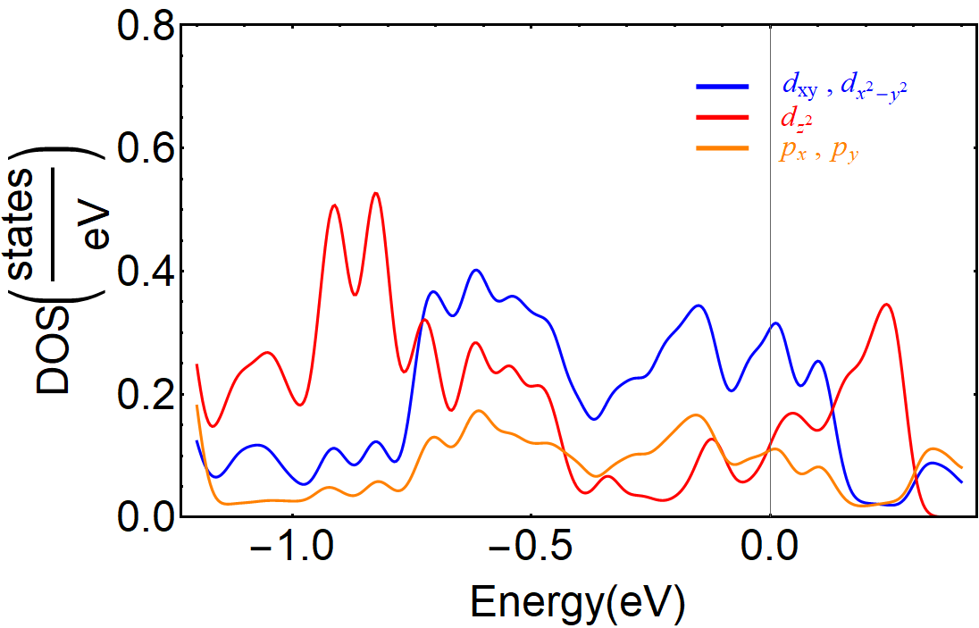
Figure 4: DOSs per atom of K₂Cr₃As₃ projected onto orbitals symmetric with respect to the basal plane, i.e. $d_{xy}$ and $d_{x^{2}-y^{2}}$ (blue line), $d_{z^{2}}$ (red line) and $p_{x}$ and $p_{y}$ (orange line). The curves have been obtained averaging the projected DOSs over all the atoms of the unit cell.

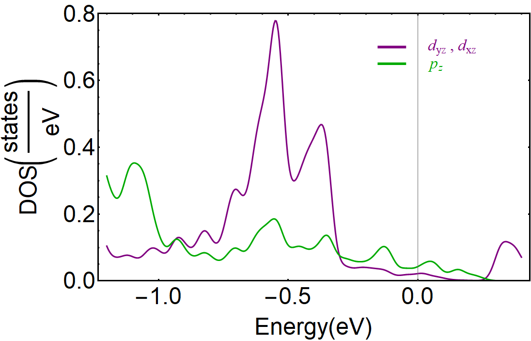
Figure 5: Same as in Fig.4 for antisymmetric orbitals, i.e. $d_{yz}$ and $d_{xz}$ (purple line) and $p_{z}$ (green line).

Their behavior confirms the results of first-principle calculations, namely the orbitals that dominate the low-energy excitations are the chromium $d_{xy}$, $d_{x^{2}-y^{2}}$ and $d_{z^{2}}$ (Jiang15, ), with the highest contribution corresponding to a pronounced peak at the Fermi energy associated with the $d_{xy}$ and $d_{x^{2}-y^{2}}$ orbitals. Nonetheless, we see that an appreciable contribution also comes from As $p_{x}$ and $p_{y}$ orbitals, this signaling the difficulty of reducing the full Hamiltonian (2) to a simpler effective one where the $d$ and the $p$ orbital degrees of freedom are efficiently disentangled. Finally, from Fig. 5 we see that the projected DOS for antisymmetric orbitals exhibits negligible contribution at the Fermi energy, providing evidence of the decoupling between the two sectors corresponding to orbitals symmetric or antisymmetric with respect to the basal plane.

To gain a better insight into the nature of the isolated set of ten bands in the energy window [-1.2 eV, 0.4 eV] around the Fermi level, we have performed a detailed analysis of the orbital character of each energy level along the main directions in the Brillouin zone. This is provided through the "fat bands" representation, where the width of each band-line is proportional to the weight of the corresponding orbital component, as shown in Figs. 6-10. One can notice that an accurate description of the conduction and valence bands along the various paths involves both Cr and As. As one can see, the three bands crossing the Fermi level are mainly built from the $d_{xy}$, $d_{x^{2}-y^{2}}$, $d_{z^{2}}$ orbitals of Cr, with a degree of mixing which is highly dependent on the selected path in the Brillouin zone.

Figure 6: Contribution to the tight binding band structure (blue curve) of the $d_{xy}$ and $d_{x^{2}-y^{2}}$ orbitals, represented as fat band (in orange).

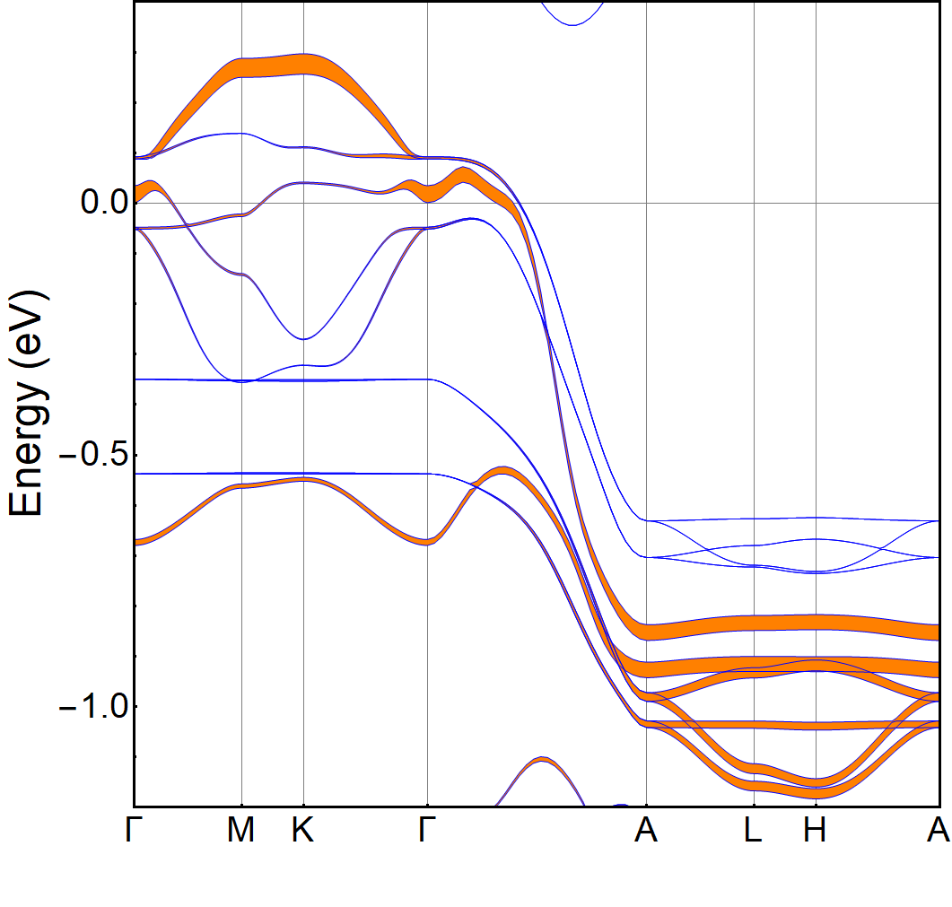
Figure 7: Same as in Fig.6, referred to the $d_{z^{2}}$ orbital.

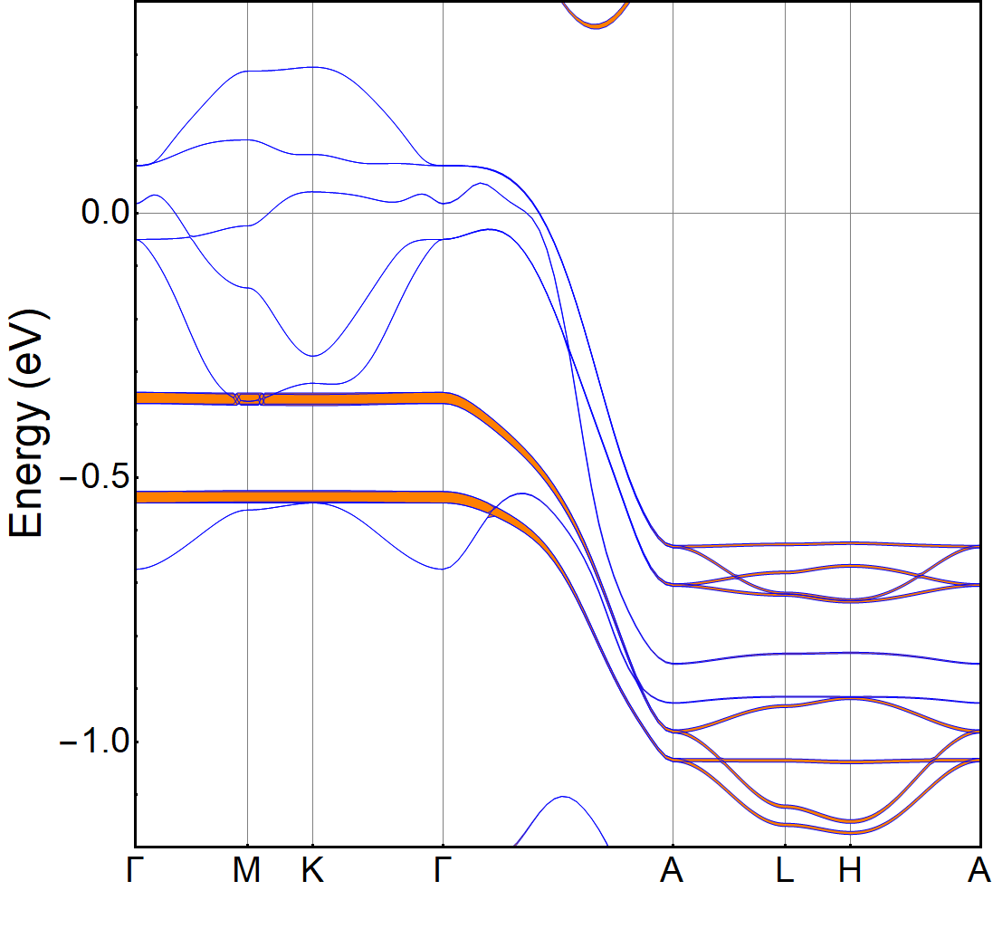
Figure 8: Same as in Fig.6, referred to the $d_{xz}$ and $d_{yz}$ orbitals.

Figure 9: Same as in Fig.6, referred to the $p_{x}$ and $p_{y}$ orbitals.

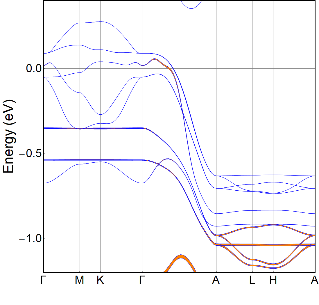
Figure 10: Same as in Fig.6, referred to the $p_{z}$ orbital.

IV Löwdin procedure

As our previous analysis suggests, the symmetric orbitals $d_{xy}$, $d_{x^{2}-y^{2}}$, $d_{z^{2}}$, $p_{x}$ and $p_{y}$ dominate at the Fermi level, so one can project out the low-lying degrees of freedom using the Löwdin downfolding procedure (lowdin50, ). This method is based on the partition of a basis of unperturbed eigenstates into two classes, related to each other by a perturbative formula giving the influence of one class of states on the other one. In this case, the two classes are the symmetric (s) and antisymmetric (a) $p$ and $d$ orbitals with respect to the basal plane.

Schematically, given the basis defined in Eq.(1), the matrix has the structure

$$H=\left[\begin{array}[]{c|c}H_{ss}&H_{sa}\\ \hline\cr H_{as}&H_{aa}\end{array}\right]\,,$$ (6)

where $H_{ss}$ is the submatrix including hoppings between symmetric orbitals, $H_{sa}$ hoppings between symmetric and anti-symmetric orbitals, and $H_{aa}$ hoppings between anti-symmetric orbitals.

The submatrices are in turn made of block matrices. Considering for instance $H_{ss}$, we have

$$H_{ss}=\left[\begin{array}[]{c|c}H_{Cr_{s}Cr_{s}}&H_{Cr_{s}As_{s}}\\ \hline\cr H_{As_{s}Cr_{s}}&H_{As_{s}As_{s}}\end{array}\right]\,,$$ (7)

where the subscripts indicate the orbitals involved, so that

$$H_{Cr_{s}Cr_{s}}=\begin{bmatrix}H_{xy/xy}&H_{xy/x^{2}-y^{2}}&H_{xy/z^{2}}\\ H_{x^{2}-y^{2}/xy}&H_{x^{2}-y^{2}/x^{2}-y^{2}}&H_{x^{2}-y^{2}/z^{2}}\\ H_{z^{2}/xy}&H_{z^{2}/x^{2}-y^{2}}&H_{z^{2}/z^{2}}\end{bmatrix},$$

$$H_{As_{s}As_{s}}=\begin{bmatrix}H_{x/x}&H_{x/y}\\ H_{y/x}&H_{y/y}\end{bmatrix}.$$

and similarly for $H_{Cr_{s}As_{s}}$. Here $xy$, $x^{2}-y^{2}$, $z^{2}$, $yz$ and $xz$ denote the five $d$ orbitals of the Cr atoms, while $x$, $y$ and $z$ denote the three $p$ orbitals of the As atoms. For example, $H_{xy/x^{2}-y^{2}}$ is the submatrix that includes all the hopping processes between the $d_{xy}$ and $d_{x^{2}-y^{2}}$ orbitals belonging to the six chromium atoms.

Referring to the matrix of Eq. (6) and downfolding the $H_{aa}$ submatrix, the solution of the original eigenvalue problem is mapped to that of a corresponding effective Hamiltonian $\widetilde{H}_{ss}$, whose rank is 30, with $\widetilde{H}_{ss}$ given by (andersen95, )

$$\widetilde{H}_{ss}(\varepsilon)={H}_{ss}-{H}_{sa}\left({H}_{aa}-\varepsilon\mathbb{I}\right)^{-1}{H}_{as}\,.$$ (8)

Using this technique, we get the low-energy effective Hamiltonian projected into the subsector given by the symmetric orbitals, going beyond the simpler complete Wannier function method. The band structure that we have obtained applying the Löwdin procedure is shown in Fig. 11, where the DFT spectrum near the Fermi level is also reported for comparison. We can see that the band structure near the Fermi level is caught to a high degree of approximation and the agreement is almost complete. The $d$ and $p$ anti-symmetric orbitals thus can be fully disentangled from the symmetric ones, as a consequence of the peculiar geometry corresponding to the arrangement of the chromium atoms.

It is worth noting that we still have a disagreement in the A-L-H-A region. Such an occurrence is due to the predominance of the weight of the $d_{z^{2}}$ orbital in that region of the Brillouin zone, although the corresponding bands are somehow distant from the Fermi surface.

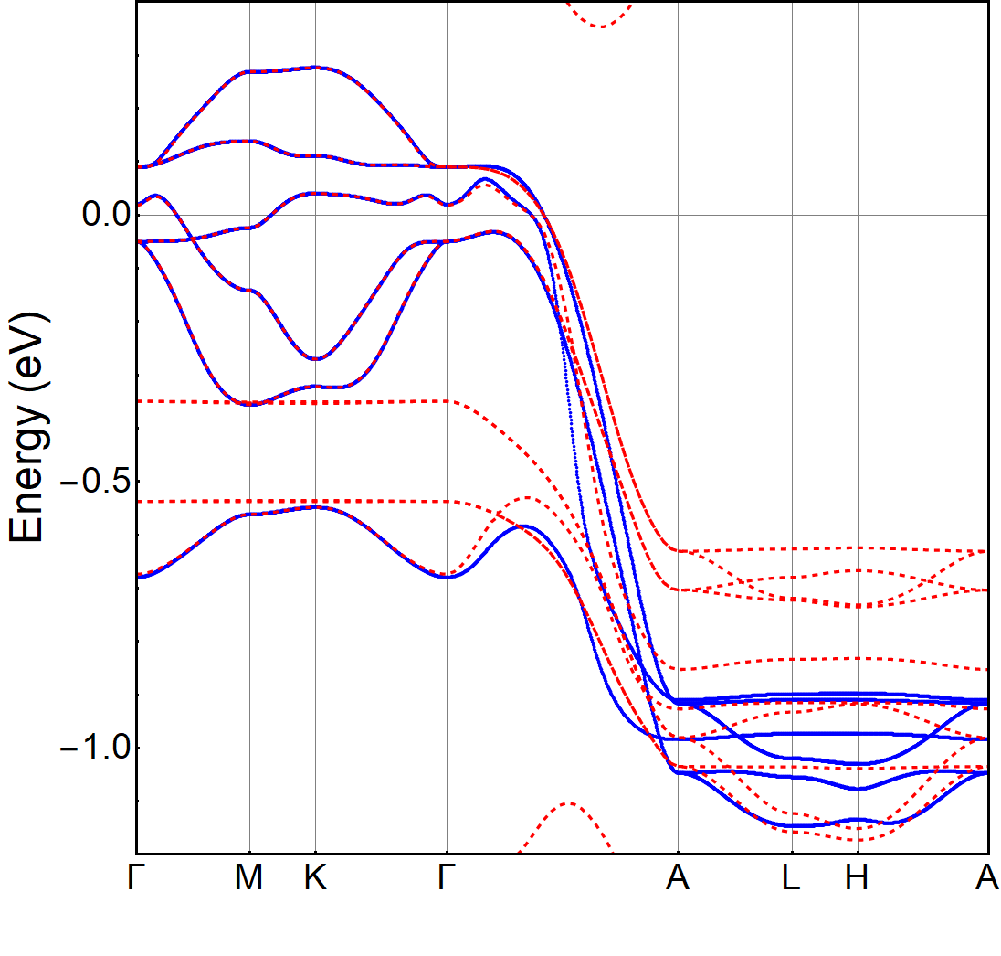
Figure 11: Comparison in the energy range around the Fermi level between the DFT band structure (red dashed lines) and the one obtained from the Löwdin downfolding procedure described in the text (blue lines).

V Derivation of a minimal five-band tight-binding model

On the basis of the indications provided by the orbital characterization of the band structure and by the Löwdin procedure, we now introduce a minimal tight-binding model allowing to satisfactorily reproduce the energy spectrum around the Fermi energy in the whole ${\bf k}$-space. We start by referring to the isolated set of ten bands developing in the energy range going approximately from -1.2 to 0.4 eV (see, for instance, Fig. 11). The fat band representation used in Figs. 6-10 provides evidence that these bands have mainly the character of the orbitals that are symmetric with respect to the basal plane. The Löwdin projection clearly demonstrated that downfolding the ten bands over the six symmetric ones, it is possible to obtain a very good description of the energy bands in proximity of the Fermi energy. These results naturally suggest a further refinement of our calculations, consisting in an application of the Wannier method taking explicitly into account the predominant weight of the symmetric states. We eventually find that this combination of the Löwdin and the Wannier approaches allows to obtain a fully reliable minimal tight-binding model.

We observe that the non-dispersive bands in the $k_{z}$=0 plane present an anti-symmetric character with weight mainly coming from $d_{xz}$ and $d_{yz}$ orbitals. Moreover, as one can see from the behavior of the DOS shown in Fig. 5, the contribution at the Fermi level of these bands, as well as the one of the $p$ bands, is small compared to that of the symmetric ones. This suggests to exclude the anti-symmetric bands from the construction of a simplified model Hamiltonian, and thus to consider only the six symmetric ones, associated with two $d_{xy}$, two $d_{x^{2}-y^{2}}$ and two $d_{z^{2}}$ orbitals. A further simplification is applied limiting to one the number of the $d_{z^{2}}$ orbital, in consideration of the fact that the corresponding band is the one lying farther from the Fermi energy. We thus perform the Wannier calculation referring to a five-band effective model, consistently with the fact that four bands cut the Fermi level, one of them being doubly degenerate at $\Gamma$ point.

Since chromium-based compounds, such as K₂Cr₃As₃, exhibit weak or moderate electronic correlations, they have a covalent character rather than a ionic one, so that, in the case of low-dimensional systems, a Wannier function can also be placed between equivalent atoms (Autieri17a, ). Our choice is to place $d_{xy}$, $d_{x^{2}-y^{2}}$, and $d_{z^{2}}$ wave functions in the middle of the Cr-triangle belonging to the KCr₃As₃ plane, locating the other two $d_{xy}$ and $d_{x^{2}-y^{2}}$ wave functions in the middle of the Cr-triangle lying in the K₃Cr₃As₃ plane. The interpolated band structure obtained by this method is shown in Fig. 12 together with the DFT band structure. We can observe a perfect match between the two spectra, thus demonstrating that our five-band model allows to describe the low energy physics in a range of about 0.3 eV around the Fermi level with the same accuracy provided by DFT. We also notice that the mixing of two different types of orbital which is at the basis of the model, suggests that K₂Cr₃As₃ might actually behave as a two-channel Stoner $d$-electron metallic magnet (Wysokinski2018, ). Interestingly, this effect can drive pressure-induced transitions between ferromagnetic and antiferromagnetic ground states.

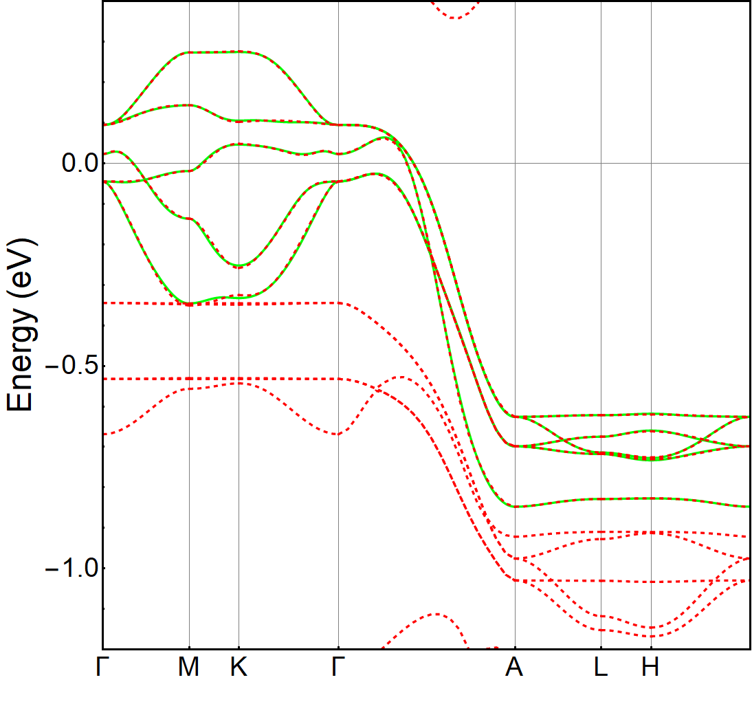
Figure 12: Comparison between the LDA band structure (red dashed lines) and the one obtained from the five-band model described in the text (green solid lines).

We now derive the analytic expression of our tight-binding model, including in the calculation three NN hopping terms along $z$, one in the plane and one along the diagonal. We will denote by $\alpha_{1}$ and $\alpha_{2}$ the Wannier functions relative to the orbitals in the plane at $z=c/2$ with predominant $xy$ and $x^{2}-y^{2}$ character, $c/2$ being the distance between KCr₃As₃ and K₃Cr₃As₃ planes, and by $\alpha_{3}$, $\alpha_{4}$ and $\alpha_{5}$ those relative to the orbitals with predominant $xy$, $x^{2}-y^{2}$ and $z^{2}$ character, respectively, in the plane with $z=0$. We will also denote by $t_{\alpha_{i},\alpha_{j}}^{lmn}$ the hopping amplitudes between the Wannier states $\alpha_{i}$ and $\alpha_{j}$ along the direction l$\mathbf{x}$ + m$\mathbf{y}$ + n$\mathbf{z}$. Since the system exhibits inversion symmetry along the $z$ axis and the orbitals under consideration are even, we will get terms proportional to $cos(nk_{z}c/2)$ for the hopping along $z$, $n$ being an even (odd) integer for hopping between homologous (different) orbitals.

According to the above assumptions, the Hamiltonian in momentum space is represented as a 5$\times$5 matrix, with elements $H_{\alpha_{i},\alpha_{j}}$. Concerning the diagonal elements, i.e. those referring to the same Wannier state, they result from the sum of different contributions related to on-site, out-of-plane and in-plane amplitudes, respectively. They thus read as

$$H_{\alpha_{i},\alpha_{i}}(k_{x},k_{y},k_{z})=H_{\alpha_{i},\alpha_{i}}^{0}+H_{\alpha_{i},\alpha_{i}}^{\perp}(k_{z})+H_{\alpha_{i},\alpha_{i}}^{\parallel}(k_{x},k_{y})$$

where

$$H_{\alpha_{i},\alpha_{i}}^{0} = t_{\alpha_{i},\alpha_{i}}^{000}\equiv\varepsilon_{\alpha_{i}}^{0}$$

$$H_{\alpha_{i},\alpha_{i}}^{\perp}(k_{z}) = \sum_{n=1,2,3}2t_{\alpha_{i},\alpha_{i}}^{00n}\cos{(nk_{z}c)}$$

$$H_{\alpha_{i},\alpha_{i}}^{\parallel}(k_{x},k_{y}) = 2t_{\alpha_{i},\alpha_{i}}^{100}\cos{(k_{x}a)}$$

$$+4t_{\alpha_{i},\alpha_{i}}^{010}\cos{(k_{x}\frac{a}{2})}\cos{(k_{y}a\frac{\sqrt{3}}{2})}\;,$$

with the numerical values of the hopping parameters being reported in Table 1.

	on site	out of plane			in plane
	000	001	002	003	100	010
$\alpha_{1}$	-86.6	154.1	-53.0	-6.3	23.0	-3.5
$\alpha_{2}$	-86.6	154.1	-53.0	-6.3	-12.3	14.2
$\alpha_{3}$	-37.0	165.0	-41.9	-2.9	30.9	-0.2
$\alpha_{4}$	-37.0	165.0	-41.9	-2.9	-10.6	20.6
$\alpha_{5}$	0	271.6	-63.9	-14.2	-15.4	-15.4

Table 1: On-site energies and out-of-plane and in-plane hopping integrals between the same Wannier states. The on-site energy of the $z^{2}$-like function is set to zero (energy units in meV).

Going to the off-diagonal elements connecting different Wannier states, we first observe on a general ground that when a crystal structure exhibits a reflection symmetry with respect to the $x$ axis, one has for pure $d$-orbitals $t_{xy,x^{2}-y^{2}}^{100}=0$ and $t_{xy,x^{2}-y^{2}}^{010}=t_{xy,x^{2}-y^{2}}^{0\bar{1}0}$. As regards K₂Cr₃As₃, we have that its crystal structure is symmetric with respect to the $y$-axis, but not with respect to the $x$-axis. Since the Wannier functions keep this missing symmetry, we have $t_{\alpha_{1},\alpha_{2}}^{100}\neq 0$ and $t_{\alpha_{1},\alpha_{2}}^{010}\neq t_{\alpha_{1},\alpha_{2}}^{0\bar{1}0}$. We stress that in our tight-binding model this effect is explicitly taken into account, differently from previous approaches where the above-mentioned $x$-axis symmetry is nonetheless applied (XWu15, ; Zhang16, ). As in the previous case, we have that the non-diagonal elements of the Hamiltonian result from in-plane and out-of-plane contributions associated with hopping processes connecting different Wannier states. Their expressions are reported in Appendix B, together with the Tables giving the numerical values of the hopping amplitudes involved.

VI Conclusions

We have presented a method that combines the Löwdin and the Wannier procedures to derive a minimal five-band tight-binding model correctly describing the low-energy physics of K₂Cr₃As₃ in terms of four planar orbitals ($d_{xy}$ and $d_{x^{2}-y^{2}}$ for each of the two planes KCr₃As₃ and K₃Cr₃As₃) and a single out-of-plane one ($d_{z^{2}}$). We are confident that this combined method can be applied to other transition-metal compounds, including the iron-based superconductors.

Our results give clear indication that the physics of the system is significantly affected by in-plane dynamics, in spite of the presence in the lattice of well-defined quasi-1D nanotube structures. The results presented here also make evident the minor role played by the local electronic correlations in determining the physical properties of the compound. Indeed, the inclusion within a LDA+U calculation scheme of a non-vanishing Hubbard repulsion developing in the Cr $d$-orbitals leads to only slight quantitative differences with respect to the non-interacting case.

We notice that although a six-band model was previously reported (Zhang16, ) using six symmetric orbitals, the five-band model proposed here describes with higher accuracy the low-energy physics as a consequence of the application of the Wannier method. We also point out that, with a filling of four electrons shared among two kinds of orbitals, the planar $d_{xy}$ and $d_{x^{2}-y^{2}}$ and the out-of-plane $d_{z^{2}}$ ones, the system might be in the Hund’s metal regime. In this framework, it has been proposed that Hund’s coupling may lead to an orbital decoupling that makes the orbitals independent from each other, so that some of them can acquire a remarkably larger mass enhancement with respect to the other ones. Furthermore, a possible connection between the orbital-selective correlations and superconductivity might be investigated: the selective correlations could be the source of the pairing glue or, alternatively, could strengthen the superconducting instability arising from a more conventional mechanism based on the exchange of bosons or spin fluctuations. Work in this direction is in progress.

Finally, we point out that the model may be used to study transport properties, magnetic instabilities, as well as superconductivity in anisotropic crystal structures (Aperis, ), also allowing to investigate dynamical effects in this class of superconductors (Demedici, ). In this case, the evidence that the main features of the energy spectrum around the Fermi level are essentially determined by the three symmetric $d_{xy}$, $d_{x^{2}-y^{2}}$ and $d_{z^{2}}$ Cr orbitals and by the $p_{x}$ and $p_{y}$ As ones, provides a constraint on the form of the superconducting order parameter that should be assumed in the development of the theory.

Appendix A Tight-binding parametrization

In this appendix, we report the systematic procedure leading to the TB parametrization based on the 48 atomic orbitals taken into account in the model Hamiltonian (2). In the following, we perform the calculations by first considering the hopping processes within the quasi one-dimensional [(Cr₃As₃)^2-]^∞ double-walled nanotubes only, and then including step by step inter-tube and longer-range intra-tube processes.

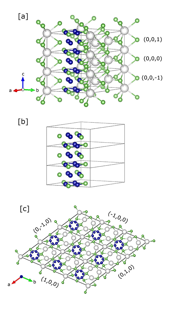
Figure 13: (a) (0,0,0), (0,0,1) and (0,0,-1) primitive cells of K₂Cr₃As₃. (b) Atoms taken into account in the diagonalization procedure when only short-range intratube hopping processes are considered. (c) (0,0,0), (1,0,0), (-1,0,0), (0,1,0), (0,-1,0), (1,-1,0), (-1,1,0), (1,1,0) and (-1,-1,0) primitive cells.

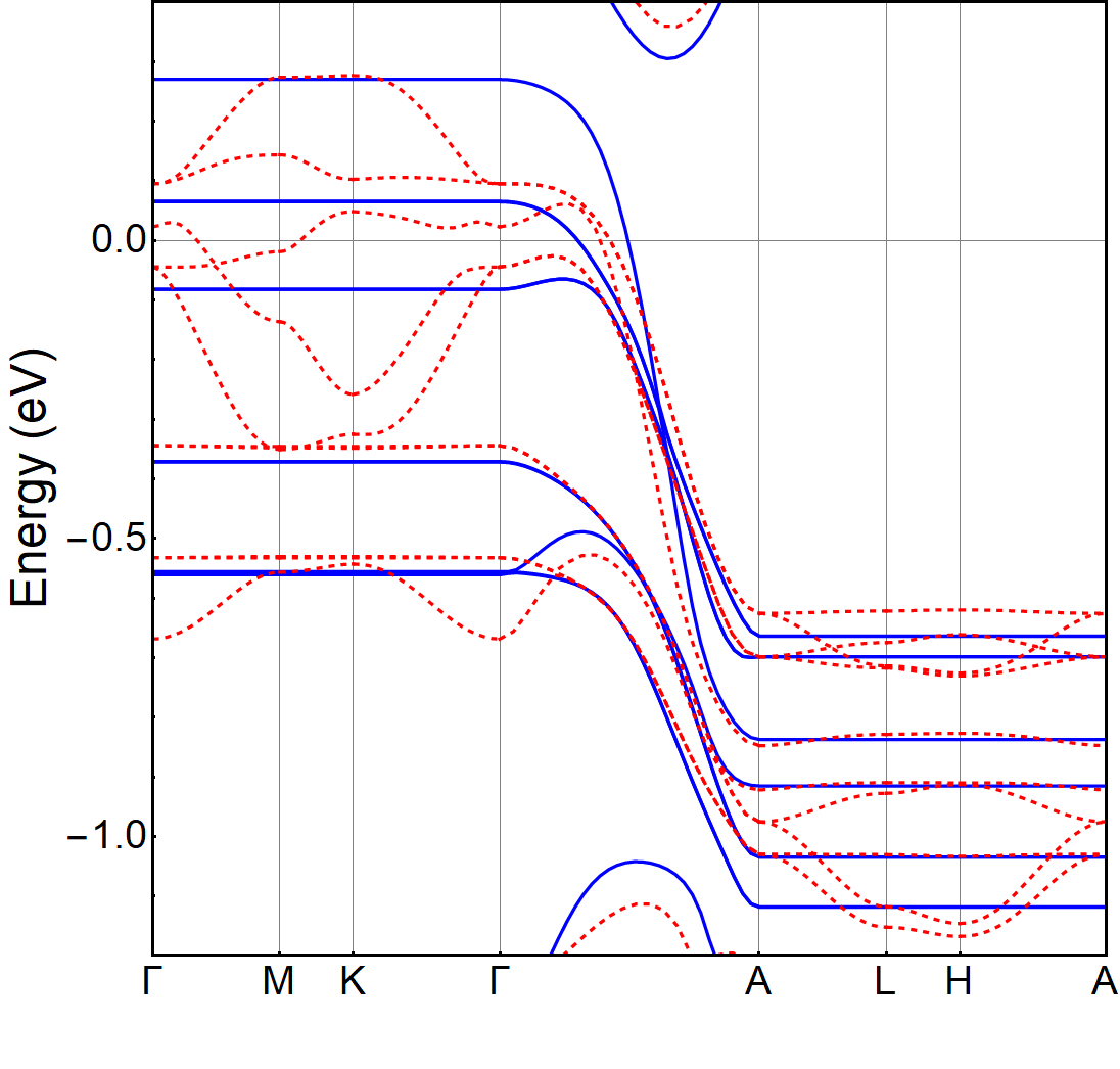
Figure 14: Comparison between the tight-binding band structure obtained considering hoppings within the (0,0,0), (0,0,1) and (0,0,-1) primitive cells (blue lines) and the DFT band structure (red dashed lines), in an energy range around the Fermi level (set equal to zero).

A.1 Short range intra-tube hybridizations

As previously pointed out, the most relevant sub-geometry of the K₂Cr₃As₃ lattice is a quasi-one dimensional double-walled sub-nanotube extending mainly along the $z$-axis. So, if we consider only hopping processes between intra-tube atoms, an already reasonable approximation of the band structure can be obtained, in particular along the line of the Brillouin zone associated with variations of $k_{z}$, i.e. the $\Gamma$-A line. Referring to the notation $\bm{R}=n_{1}\bm{a}_{1}+n_{2}\bm{a}_{2}+n_{3}\bm{a}_{3}$, we start by limiting ourselves to the primitive cells denoted by ($n_{1}$,$n_{2}$,$n_{3}$)=(0,0,0), (0,0,1) and (0,0,-1), as shown in Fig. 13(a-b).

The band structure that we have obtained is shown in Fig. 14 in an energy window around the Fermi level, with the DFT spectrum being also reported for comparison. We can see that the bands are flat along the in-plane paths of the Brillouin zone where $k_{x}$ and $k_{y}$ vary, as expected, but along the $\Gamma$-A line they exhibit a behavior quite close to the DFT results. It is also evident that more reliable results require in any case the inclusion of hopping processes involving longer range intra-tube cells as well as inter-tube ones.

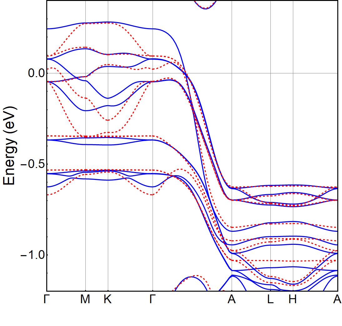
Figure 15: Same as in Fig. 14, with the tight-binding calculations extended to hopping processes in the (1,0,0), (-1,0,0), (0,1,0), (0,-1,0), (1,-1,0), (-1,1,0), (1,1,0) and (-1,-1,0) primitive cells.

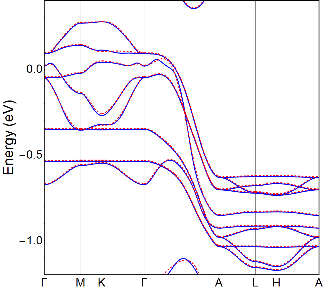
Figure 16: Same as in Fig. 15, with the tight-binding calculations further extended to fifth neighbour cells along the$z$-axis (from $n_{3}=5$ to $n_{3}=-5$) and to second-neighbor in-plane cells.

A.2 Inter-tube and long-range intra-tube hybridizations

We now include in the diagonalization procedure inter-tube hoppings in the $x$-$y$ plane ($n_{3}=0$), taking into account the contributions coming from the cells (1,0,0), (-1,0,0), (0,1,0), (0,-1,0), (1,-1,0), (-1,1,0), (1,1,0) and (-1,-1,0) (see Fig. 13(c)). The comparison of the band structure correspondingly obtained with the one given by DFT (see Fig. 15) makes evident that the agreement improves along the $\Gamma$-A line as well as along the other lines of the Brillouin zone, though there are still some qualitative differences, also at the Fermi level. In order to get a truly satisfactory agreement, it is necessary to include all hopping processes up to the fifth-neighbor cells along the z-axis (from $n_{3}=5$ to $n_{3}=-5$), together with the in-plane hoppings up to the second-neighbor cells (see Fig. 16).

Appendix B Off-diagonal elements of tight-binding Hamiltonian

We report here the expressions of the off-diagonal elements $H_{\alpha_{i},\alpha_{j}}(k_{x},k_{y},k_{z})$ $(\alpha_{i}\neq\alpha_{j})$ of the tight-binding Hamiltonian introduced in Section VI. They refer to hopping processes which connects different Wannier states and have the following form:

$$H_{\alpha_{1},\alpha_{3}} = \sum_{n=0,1,2}2t_{\alpha_{1},\alpha_{3}}^{00n+\frac{1}{2}}\cos{((n+\frac{1}{2})k_{z}c)}$$

$$+4t_{\alpha_{1},\alpha_{3}}^{100}\cos{(k_{x}a)}\cos{(k_{z}c/2)}$$

$$+4t_{\alpha_{1},\alpha_{3}}^{010}e^{i(k_{y}a\frac{\sqrt{3}}{2})}\cos{(k_{x}a/2)}\cos{(k_{z}c/2)}$$

$$+4t_{\alpha_{1},\alpha_{3}}^{0\bar{1}0}e^{-i(k_{y}a\frac{\sqrt{3}}{2})}\cos{(k_{x}a/2)}\cos{(k_{z}c/2)}$$

$$H_{\alpha_{2},\alpha_{4}} = \sum_{n=0,1,2}2t_{\alpha_{2},\alpha_{4}}^{00n+\frac{1}{2}}\cos{((n+\frac{1}{2})k_{z}c)}$$

$$+4t_{\alpha_{2},\alpha_{4}}^{100}\cos{(k_{x}a)}\cos{(k_{z}c/2)}$$

$$+4t_{\alpha_{2},\alpha_{4}}^{010}e^{i(k_{y}a\frac{\sqrt{3}}{2})}\cos{(k_{x}a/2)}\cos{(k_{z}c/2)}$$

$$+4t_{\alpha_{2},\alpha_{4}}^{0\bar{1}0}e^{-i(k_{y}a\frac{\sqrt{3}}{2})}\cos{(k_{x}a/2)}\cos{(k_{z}c/2)}$$

$$H_{\alpha_{1},\alpha_{2}} = 2it_{\alpha_{1},\alpha_{2}}^{100}\sin{(k_{x}a)}+2it_{\alpha_{1},\alpha_{2}}^{010}e^{i(k_{y}a\frac{\sqrt{3}}{2})}\sin{(k_{x}a/2)}$$

$$+2it_{\alpha_{1},\alpha_{2}}^{0\bar{1}0}e^{-i(k_{y}a\frac{\sqrt{3}}{2})}\sin{(k_{x}a/2)}$$

$$H_{\alpha_{1},\alpha_{4}} = 4it_{\alpha_{1},\alpha_{4}}^{100}\sin{(k_{x}a)}\cos{(k_{z}c/2)}$$

$$+4it_{\alpha_{1},\alpha_{4}}^{010}e^{i(k_{y}a\frac{\sqrt{3}}{2})}\sin{(k_{x}a/2)}\cos{(k_{z}c/2)}$$

$$+4it_{\alpha_{1},\alpha_{4}}^{0\bar{1}0}e^{-i(k_{y}a\frac{\sqrt{3}}{2})}\sin{(k_{x}a/2)}\cos{(k_{z}c/2)}$$

$$H_{\alpha_{1},\alpha_{5}} = 4it_{\alpha_{1},\alpha_{5}}^{100}\sin{(k_{x}a)}\cos{(k_{z}c/2)}$$

$$+4it_{\alpha_{1},\alpha_{5}}^{010}e^{i(k_{y}a\frac{\sqrt{3}}{2})}\sin{(k_{x}a/2)}\cos{(k_{z}c/2)}$$

$$+4it_{\alpha_{1},\alpha_{5}}^{0\bar{1}0}e^{-i(k_{y}a\frac{\sqrt{3}}{2})}\sin{(k_{x}a/2)}\cos{(k_{z}c/2)}$$

$$H_{\alpha_{2},\alpha_{3}} = 4it_{\alpha_{2},\alpha_{3}}^{100}\sin{(k_{x}a)}\cos{(k_{z}c/2)}$$

$$+4it_{\alpha_{2},\alpha_{3}}^{010}e^{i(k_{y}a\frac{\sqrt{3}}{2})}\sin{(k_{x}a/2)}\cos{(k_{z}c/2)}$$

$$+4it_{\alpha_{2},\alpha_{3}}^{0\bar{1}0}e^{-i(k_{y}a\frac{\sqrt{3}}{2})}\sin{(k_{x}a/2)}\cos{(k_{z}c/2)}$$

$$H_{\alpha_{2},\alpha_{5}} = 4t_{\alpha_{2},\alpha_{5}}^{100}\cos{(k_{x}a)}\cos{(k_{z}c/2)}$$

$$+4t_{\alpha_{2},\alpha_{5}}^{010}e^{i(k_{y}a\frac{\sqrt{3}}{2})}\cos{(k_{x}a/2)}\cos{(k_{z}c/2)}$$

$$+4t_{\alpha_{2},\alpha_{5}}^{0\bar{1}0}e^{-i(k_{y}a\frac{\sqrt{3}}{2})}\cos{(k_{x}a/2)}\cos{(k_{z}c/2)}$$

$$H_{\alpha_{3},\alpha_{4}} = 2it_{\alpha_{3},\alpha_{4}}^{100}\sin{(k_{x}a)}+2it_{\alpha_{3},\alpha_{4}}^{010}e^{i(k_{y}a\frac{\sqrt{3}}{2})}\sin{(k_{x}a/2)}$$

$$+2it_{\alpha_{3},\alpha_{4}}^{0\bar{1}0}e^{-i(k_{y}a\frac{\sqrt{3}}{2})}\sin{(k_{x}a/2)}$$

$$H_{\alpha_{3},\alpha_{5}} = 2it_{\alpha_{3},\alpha_{5}}^{100}\sin{(k_{x}a)}+2it_{\alpha_{3},\alpha_{5}}^{010}e^{i(k_{y}a\frac{\sqrt{3}}{2})}\sin{(k_{x}a/2)}$$

$$+2it_{\alpha_{3},\alpha_{5}}^{0\bar{1}0}e^{-i(k_{y}a\frac{\sqrt{3}}{2})}\sin{(k_{x}a/2)}$$

$$H_{\alpha_{4},\alpha_{5}} = 2t_{\alpha_{4},\alpha_{5}}^{100}\cos{(k_{x}a)}+2t_{\alpha_{4},\alpha_{5}}^{010}e^{i(k_{y}a\frac{\sqrt{3}}{2})}\cos{(k_{x}a/2)}$$

$$+2t_{\alpha_{4},\alpha_{5}}^{0\bar{1}0}e^{-i(k_{y}a\frac{\sqrt{3}}{2})}\cos{(k_{x}a/2)}$$

The numerical values of the hopping parameters in the above expressions are reported in Tables 2 and 3. In particular we see from Table 3 that the most relevant hopping amplitudes, larger than 30 meV, occur between the planar $\alpha_{1}$ and $\alpha_{2}$ and between the planar $\alpha_{3}$ and $\alpha_{4}$ Wannier states in the $xy$ plane.

	out of plane			in plane
	001	002	003	100	010	$0\bar{1}0$
$\alpha_{1}\alpha_{3}$	7.9	7.3	14.6	-7.4	-6.9	1.4
$\alpha_{2}\alpha_{4}$	7.9	7.3	14.6	-1.2	-1.7	-9.9

Table 2: Hopping integrals between $\alpha_{1}$-$\alpha_{3}$ and $\alpha_{2}$-$\alpha_{4}$ Wannier states (energy units in meV).

	100	010	$0\bar{1}0$
$\alpha_{1}\alpha_{2}$	-15.0	30.3	-0.2
$\alpha_{1}\alpha_{4}$	-7.1	-2.7	2.6
$\alpha_{1}\alpha_{5}$	-9.1	-8.6	-0.5
$\alpha_{2}\alpha_{3}$	-2.4	-7.3	-2.1
$\alpha_{2}\alpha_{5}$	-4.7	-5.6	10.2
$\alpha_{3}\alpha_{4}$	17.4	0.6	-35.4
$\alpha_{3}\alpha_{5}$	13.0	-1.0	14.1
$\alpha_{4}\alpha_{5}$	-8.7	15.7	-6.9

Table 3: Hopping integrals between different Wannier states, other than those listed in Table II (energy units in meV).

References

- (1) Chen R Y and Wang N L 2019 Rep. Prog. Phys. 82 012503
- (2) Wu W, Zhang X, Yin Z, Zheng P, Wang N and Luo J 2010 Science China Physics, Mechanics & Astronomy 53 1207
- (3) Wu W, Cheng J, Matsubayashi K, Kong P, Lin F, Jin C, Wang N, Uwatoko Y and Luo J 2014 Nat. Commun. 5 5508
- (4) Kotegawa H, Nakahara S, Tou H and Sugawara H 2014 J. Phys. Soc. Japan 83 093702
- (5) Nigro A, Marra P, Autieri C, Wu W, Cheng J C, Luo J and Noce C 2018 arXiv:1812.09957v1[cond-mat.str-el]
- (6) Bao J-K, Liu J-Y, Ma C-W, Meng Z-H, Tang Z-T, Sun Y-L, Zhai H-F, Jiang H, Bai H, Feng C-M, Xu Z-A and Cao G-H 2015 Phys. Rev. X 5 011013
- (7) Tang Z-T, Bao J-K, Liu Y, Sun Y-L, Ablimit A, Zhai H-F, Jiang H, Feng C-M, Xu Z-A and Cao G-H 2015 Phys. Rev. B 91 020506(R)
- (8) Tang Z-T, Bao J-K, Wang Z, Bai H, Jiang H, Liu Y, Zhai H-F, Feng C-M, Xu Z-A and Cao G-H 2015 Sci. China Mater. 58 16
- (9) Mu Q-G, Ruan B-B, Pan B-J, Liu T, Yu J, Zhao K, Chen G-F and Ren Z-A 2018 Phys. Rev. Materials 2 034803
- (10) Kong T, Bud’ko S L and Canfield P C 2015 Phys. Rev. B 91 020507(R)
- (11) Zhi H Z, Imai T, Ning F L, Bao J-K and Cao G-H 2015 Phys. Rev. Lett. 114 147004
- (12) Adroja D T, Bhattacharyya A, Telling M, Feng Y, Smidman M, Pan B, Zhao J, Hillier A D, Pratt F L and Strydom A M 2015 Phys. Rev. B 92 134505
- (13) Pang G M, Smidman M, Jiang W B, Bao J K, Weng Z F, Jiao L, Zhang J L, Cao G H and Yuan H Q 2015 Phys. Rev. B 91 220502(R)
- (14) Watson M D, Feng Y, Nicholson C W, Monney C, Riley J M, Iwasawa H, Refson K, Sacksteder V, Adroja D T, Zhao J and Hoesch M 2017 Phys. Rev. Lett. 118 097002
- (15) Jiang H, Cao G and Cao C 2015 Sci. Rep. 5 16054
- (16) Taddei K M, Zheng Q, Sefat A S and de la Cruz C 2017 Phys. Rev. B 96 180506(R)
- (17) Taddei K M, Xing G, Sun J, Fu Y, Li Y, Zheng Q, Sefat A S, Singh D J and de La Cruz C 2018 Phys. Rev. Lett. 121 187002
- (18) Wu X, Fang F, Le C, Fan H and Hu J 2015 Phys. Rev. B 92 104511
- (19) Zhang L-D, Wu X, Fan H, Yang F and Hu J 2016 Europhys. Lett. 113 37003
- (20) Zhong H, Feng X-Y, Chen H and Dai J 2015 Phys. Rev. Lett. 115 227001
- (21) Zhou Y, Cao C and Zhang F-C 2017 Sci. Bull. 62 208
- (22) Autieri C and Noce C 2017 Phil. Mag. 97 3276
- (23) Kresse G and Hafner J 1993 Phys. Rev. B 47 558 Kresse G and Hafner J 1994 Phys. Rev. B 49 14251 Kresse G and Furthmüller J 1996 Phys. Rev. B 54 11169 Kresse G and Furthmüller 1996 Comput. Mat. Sci. 6 15
- (24) Kresse G and Joubert D 1999 Phys. Rev. B 59 1758
- (25) Predew J P and Zunger A 1981 Phys. Rev. B 23 5048
- (26) Ceperley D M and Alder B J 1980 Phys. Rev. Lett. 45 566
- (27) Marzari N and Vanderbilt D 1997 Phys. Rev. B 56 12847
- (28) Souza I, Marzari N and Vanderbilt D 2001 Phys. Rev. B 65 035109
- (29) Mostofi A A, Yates J R, Lee Y S, Souza I, Vanderbilt D and Marzari N 2008 Comput. Phys. Comm. 178 685
- (30) Anisimov V I, Solovyev I V, Korotin M A, Czyzyk M T and Sawatzky G A 1993 Phys. Rev. B 48 16929
- (31) Vaugier L, Jiang H and Biermann S 2012 Phys. Rev. B 86 165105
- (32) Autieri C, Cuono G, Forte F and Noce C 2017 J. Phys.: Condens. Matter 29 224004
- (33) Autieri C, Cuono G, Forte F and Noce C 2018 J. Phys.: Conf. Ser. 969 012106
- (34) Cuono G, Autieri C, Forte F, Busiello G, Mercaldo M T, Romano A, Noce C and Avella A 2018 AIP Advances 8 101312
- (35) Setyawan W and Curtarolo S 2010 Comput. Mater. Sci. 49 299
- (36) Löwdin P O 1950 J. Chem. Phys. 18 365
- (37) Andersen O K, Liechtenstein A I, Jepsen O and Paulsen F 1995 J. Phys. Chem. Solids 56 1573
- (38) Autieri C, Bouhon A and Sanyal B 2017 Phil. Mag. 97 3381
- (39) Wysokinski M 2018 arXiv:1808.04109v2 [cond-mat.str-el]
- (40) Aperis A, Maldonado P and Oppeneer P M 2015 Phys. Rev. B 92 054516
- (41) Edelmann M, Sangiovanni G, Capone M and de’ Medici L 2017 Phys. Rev. B 95 205118