Approximation to Singular Quadratic Collision Model in Fokker-Planck-Landau Equation

Abstract

We propose a Hermite-Galerkin spectral method to numerically solve the spatially homogeneous Fokker-Planck-Landau equation with singular quadratic collision model. To compute the collision model, we adopt a novel approximation formulated by a combination of a simple linear term and a quadratic term very expensive to evaluate. Using the Hermite expansion, the quadratic term is evaluated exactly by calculating the spectral coefficients. To deal with singularities, we make use of Burnett polynomials so that even very singular collision model can be handled smoothly. Numerical examples demonstrate that our method can capture low-order moments with satisfactory accuracy and performance.

Keywords: Fokker-Planck-Landau equation; Hermite-Galerkin spectral method; Burnett polynomials; Quadratic collision operator; Super singularity

1 Introduction

The Fokker-Planck-Landau (FPL) equation is a common kinetic model in plasma physics, accelerator physics and astrophysics. It describes binary collision between charged particles with long-range Coulomb interaction, and is represented by a nonlinear partial integro-differential equation.

As a classical result, the FPL operator is the limit of the Boltzmann operator for a sequence of scatting cross sections which converge in a convenient sense to a delta function at zero scattering angle [8]. The original derivation of the equation based on this idea is due to Landau [22], and then several work has been devoted to this problem, such as [2, 12, 29]. Recently Villani [33] has obtained a rigorous proof of this asymptotic problem in the space homogeneous scenario. For the mathematical properties of the FPL equation, such as the existence of the solutions, we refer the reader to Villani [32] and the reference therein.

The numerical solution of the nonlinear kinetic equations, such as FPL equation, also represents a real challenge for numerical method. This is essentially due to the non-linearity, as well as the high dimension of variables, which is seven for the full problem. Moreover, the complex three dimensional integro-differential stiff advection-diffusion operator in velocity space is also remarkably difficult to deal with due to the high singularity. Besides, this integration has to be handled carefully since it is closely related to the macroscopic properties, for example the collision term does not change the total mass, momentum and energy. Several numerical approaches have been brought up to solve FPL equation. Generally speaking, there are two kinds of methods, stochastic methods and the deterministic methods. For the stochastic methods, DSMC method which is widely in the simulation of Boltzmann equation[4] is adopted to solve FPL equation. A detail discussion about the stochastic method is beyond the scope of this paper, and we refer the reader to [15, 5] for a much more complete treatment. For the deterministic methods, due to the complex form of the FPL operator, several numerical approaches are devoted to the simpler diffusive Fokker-Planck model [17, 37], the space homogeneous situations in the isotropic case [6] or cylindrically symmetric problems [26]. Moreover, Villani [34] has brought up a linear collision model for the Maxwell molecules. The construction of conservative and entropy schemes for the space homogeneous case has been proposed in [13, 7], where the main physical properties are all satisfied. But the direct implementation of such schemes are all quite expensive. Several fast approximated algorithms to reduce the complexity of these methods, based on multipole expansion [23] or multigrid techniques [6] have been proposed. A fast spectral method based on Fourier spectral approximation of the collision operator is introduced in [25], and it is then also utilized to solve inhomogeneous FPL equation [36, 16]. For the numerical stiffness of the Fokker-Planck collision operator, the implicit time scheme is also studied [24, 31]. There is a certain kind of asymptotic-preserving method that seeks to accelerate the solution of the FPL equation by the so-called penalization techniques [21].

As another kind of spectral method, Hermite spectral method is also utilized to solve FPL equation. Hermite method, where the basis functions with weighted orthogonality in $\mathbb{R}^{3}$ are employed, dates back to Grad’s work [19] where it is used to solve the Boltzmann equation and is known as the moment method ever since. Besides, the expansion with respect to Burnett polynomials was proposed in [9, 18] to find the coefficients of the collision term of the expansion in the Hermite basis. Using the Hermite expansion, it is still a tough job to evaluate the exact coefficients in the expansion of the collision operator, since the computational cost for the quadratic from is hardly bearable and novel models need to be introduced. In a recent work [35], the explicit expressions of all the coefficients in the Hermite spectral method for the quadratic Boltzmann collision operator are presented, and the new collision model which can preserve the physical properties and reduce computational cost at the same time was brought up using these coefficients. It is much harder to evaluate these coefficients for the quadratic FPL collision operator compared to the Boltzmann equation, because of the high singularity and the operator of partial derivative. In [27], the coefficients for the Coulombian case were evaluated numerically, and the explicit form was listed for the first few moments.

Inspired by these work, we in this paper are devoted to the numerical method for FPL equation with quadratic collision model, which may be very singular. Following the approach in [35], we approximate the collision model as the combination of a simple linear term and a quadratic term. The idea is to take only a portion in the truncated series expansion to be treated “quadratically”, and the remaining part is approximated by the linear collision operator brought up by Villani [34]. This may greatly reduce the computational cost and we can still capture the evolution of physical variables accurately. The linear term can be handled easily, while the difficulty imposed by the singularity in the quadratic collision model remains. We reveal that by making use of Burnett polynomials, the singular part of the integral in the collision operator can be handled smoothly. For the typical case that the repulsive force between molecules is proportional to a negative power of their distance, our method can handle problems where the index for the power of distance is as great as $-5$, in comparison to the index fixed as $-3$ in [27]. To deal with the remaining part in the quadratic term without singularity, the Hermite-Galerkin spectral method is then adopted. We derive the explicit formulae for all the coefficients in the Hermite expansion of the collision operator, and these formulae can all be evaluated exactly offline for immediate applications. Thus eventually the quadratic term is able to be evaluated efficiently.

The rest of this paper is organized as follows. In Section 2, we briefly review the FPL equation and the Hermite expansion of the distribution function. In Section 3, we first give an explicit expression of the series expansion of the quadratic collision operator and then introduce precisely how to deal with the singularity by Burnett polynomials. The construction of the approximated collision model is presented in Section 4. Some numerical experiments verifying the effectiveness of our methods are carried out in Section 5. The concluding remarks and detailed derivation of the expansions are given in Section 6 and 7 respectively.

2 FPL equation and Hermite expansion

We will first give a brief review of the FPL equation, and then introduce the Hermite spectral method for the expansion of the distribution function.

2.1 FPL equation

The Fokker-Planck-Landau equation is a prevalent kinetic model in plasma physics, describing the state of the particles in terms of a distribution function $f(t,\boldsymbol{x},\boldsymbol{v})$, where $t$ is the time coordinate, $\boldsymbol{x}$ represents the spatial coordinates, and $\boldsymbol{v}$ stands for the velocity of particles. The governing equation of $f$ is

$$\frac{\partial f}{\partial t}+\nabla_{\boldsymbol{x}}\cdot(\boldsymbol{v}f)=\mathcal{Q}[f],\qquad t\in\mathbb{R}^{+},\quad\boldsymbol{x}\in\mathbb{R}^{3},\quad\boldsymbol{v}\in\mathbb{R}^{3},$$ (2.1)

where $\mathcal{Q}[f]$ is the collision operator with a quadratic form

$$\mathcal{Q}[f](t,\boldsymbol{x},\boldsymbol{v})=\nabla_{\boldsymbol{v}}\cdot\int_{\mathbb{R}^{3}}A(\boldsymbol{v}-\boldsymbol{v}_{\ast})(f(\boldsymbol{v}_{\ast})\nabla_{\boldsymbol{v}}f(\boldsymbol{v})-f(\boldsymbol{v})\nabla_{\boldsymbol{v}_{\ast}}f(\boldsymbol{v}_{\ast}))\,\mathrm{d}\boldsymbol{v}_{\ast},$$ (2.2)

where $A$ depends on the interaction between particles and is a $3\times 3$ negative and symmetric matrix in the form [25] of

$$A(\boldsymbol{v})=\Psi(|\boldsymbol{v}|)\Pi(\boldsymbol{v}),$$ (2.3)

where $\Psi$ is a non-negative radial function, and $\Pi(\boldsymbol{v})$ is the orthogonal projection upon the space orthogonal to $\boldsymbol{v}$, as $\Pi_{ij}(\boldsymbol{v})=\delta_{ij}-\frac{v_{i}v_{j}}{|\boldsymbol{v}|^{2}}$.

We are primarily concerned with the IPL model, for which the force between two molecules is always repulsive and proportional to a negative power of their distance. In this case, the function $\Psi(\boldsymbol{v})$ has the form

$$\Psi(\boldsymbol{v}):=\Lambda|\boldsymbol{v}|^{\gamma+2},$$ (2.4)

where $\Lambda>0$ is a constant and $\gamma$ is the index of the power of distance. This equation is obtained as a limit of the Boltzmann equation, when all the collisions become grazing [14]. In the case of the Boltzmann equation, different $\gamma$ lead to different models. The case $\gamma>0$ corresponds to the “hard potential” case, whereas for $\gamma<0$, it corresponds to the case of “soft potential”. In the critical case $\gamma=0$, the gas molecules are referred to as “Maxwell molecules”. Another case of interest is when $\gamma=-3$ of the Coulombian case, which is a very important model for applications in plasma.

We shall focus on the numerical approximation of $\mathcal{Q}[f]$, especially when $\gamma$ is very small. Our model of approximating the collision operator is best illustrated in the spatially homogeneous FPL equation case, namely

$$\frac{\partial f}{\partial t}=\mathcal{Q}[f],\qquad t\in\mathbb{R}^{+},\quad\boldsymbol{v}\in\mathbb{R}^{3}.$$ (2.5)

As a classical result in kinetic equations, the steady state solution of this equation takes the form of the Maxwellian:

$$\mathcal{M}_{\rho,\boldsymbol{u},\theta}(\boldsymbol{v}):=\frac{\rho}{(2\pi\theta)^{3/2}}\exp\left(-\frac{|\boldsymbol{v}-\boldsymbol{u}|^{2}}{2\theta}\right),$$ (2.6)

where the density $\rho$, velocity $\boldsymbol{u}$ and temperature $\theta$ are defined as follows

$$\rho=\int_{\mathbb{R}^{3}}f(t,\boldsymbol{v})\,\mathrm{d}\boldsymbol{v},\quad\boldsymbol{u}=\frac{1}{\rho}\int_{\mathbb{R}^{3}}\boldsymbol{v}f(t,\boldsymbol{v})\,\mathrm{d}\boldsymbol{v},\quad\theta=\frac{1}{3\rho}\int_{\mathbb{R}^{3}}|\boldsymbol{v}-\boldsymbol{u}|^{2}f(t,\boldsymbol{v})\,\mathrm{d}\boldsymbol{v}.$$ (2.7)

Moreover, the physical variables such as the heat flux $q_{i}$ and the stress tensor $\sigma_{ij}$ are also of interest. They are defined as

$$q_{i}=\frac{1}{2}\int_{\mathbb{R}^{3}}|\boldsymbol{v}-\boldsymbol{u}|^{2}(v_{i}-u_{i})f\,\mathrm{d}\boldsymbol{v},\qquad i=1,2,3,$$

$$\sigma_{ij}=\int_{\mathbb{R}^{3}}\left((v_{i}-u_{i})(v_{j}-u_{j})-\frac{1}{3}\delta_{ij}|\boldsymbol{v}-\boldsymbol{u}|^{2}\right)f\,\mathrm{d}\boldsymbol{v},\quad i,j=1,2,3.$$

Similar to the Boltzmann equation, the collision operator preserves in time the macroscopic quantities mass, momentum and energy. Therefore, those are invariant quantities under evolution, and (2.7) holds for any $t$. Thus we can obtain

$$\rho=1,\quad\boldsymbol{u}=0,\quad\theta=1,$$ (2.8)

by selecting proper frame of reference and applying appropriate non-dimensionalization. Now the Maxwellian (2.6) is simply reduced to

$$\mathcal{M}(\boldsymbol{v}):=\frac{1}{(2\pi)^{3/2}}\exp\left(-\frac{|\boldsymbol{v}|^{2}}{2}\right).$$ (2.9)

The heat flux and stress tensor are reduced into

$$q_{i}=\frac{1}{2}\int_{\mathbb{R}^{3}}|\boldsymbol{v}|^{2}v_{i}f\,\mathrm{d}\boldsymbol{v},\qquad\sigma_{ij}=\int_{\mathbb{R}^{3}}\left(v_{i}v_{j}-\frac{1}{3}\delta_{ij}|\boldsymbol{v}|^{2}\right)f\,\mathrm{d}\boldsymbol{v},\quad i,j=1,2,3.$$

The normalization (2.8) shall always be assumed in the following context.

In the literature, the complicated form of the collision operator $\mathcal{Q}[f]$ is handled by introducing approximations of less complexity. For instance, for the Maxwell molecules with $\Lambda=1$, if the distribution function $f$ is radially symmetric, which is a property to be preserved under time evolution, the collision operator can be rewritten as

$$\mathcal{Q}^{\mathrm{linear}}[f]=(D-1)\nabla_{\boldsymbol{v}}\cdot(\nabla f+f\boldsymbol{v}),$$ (2.10)

which was proposed by C. Villani [34] . Here $D$ is the dimension of the velocity space, and we always set $D=3$ in the context. In this case, the FPL equation is reduced into the linear Fokker-Planck equation (FP), which can be used to describe the relation of Brownian molecules in a gas.

Due to the complex form of the FPL operator, several numerical approaches are devoted to the simpler diffusive Fokker-Planck model or on the reduced collision models [28, 3]. Hence it is of high necessity to develop efficient numerical methods for the original FPL equation with quadratic collision operator.

2.2 Series expansion of distribution function

Our numerical discretization shall be based on the series expansion in the weighted $L^{2}$ space of the distribution function $\mathcal{F}=L^{2}(\mathbb{R}^{3};\mathcal{M}^{-1}\,\mathrm{d}\boldsymbol{v})$:

$$f(t,\boldsymbol{v})=\sum_{|{\alpha}|=0}^{+\infty}f_{{\alpha}}(t)H^{{\alpha}}(\boldsymbol{v})\mathcal{M}(\boldsymbol{v}),$$ (2.11)

where $\mathcal{M}(\boldsymbol{v})$ is the Maxwellian, and ${\alpha}=(\alpha_{1},\alpha_{2},\alpha_{3})^{T}$ is a three-dimensional multi-index, and $|{\alpha}|=\alpha_{1}+\alpha_{2}+\alpha_{3}$. In (2.11), $H^{{\alpha}}(\boldsymbol{v})$ are the Hermite polynomials defined as follows:

Definition 1 (Hermite polynomials).

For $\alpha_{i}\in\mathbb{N},i=1,2,3$, the Hermite polynomial $H^{{\alpha}}(\boldsymbol{v})$ is defined as

$$H^{{\alpha}}(\boldsymbol{v})=\frac{(-1)^{n}}{\mathcal{M}(\boldsymbol{v})}\frac{\partial^{|{\alpha}|}}{\partial v_{1}^{\alpha_{1}}\partial v_{2}^{\alpha_{2}}\partial v_{3}^{\alpha_{3}}}\mathcal{M}(\boldsymbol{v}),$$ (2.12)

where $\mathcal{M}(\boldsymbol{v})$ is given in (2.9).

The expansion (2.2) was introduced to solve Boltzmann equations [19], where such an expansion was invoked to deploy moment methods. We can derive moments based on the coefficients $f_{{\alpha}}$ from the orthogonality of Hermite polynomials

$$\int_{\mathbb{R}^{3}}H^{{\alpha}}(\boldsymbol{v})H^{{\beta}}(\boldsymbol{v})\mathcal{M}(\boldsymbol{v})\,\mathrm{d}\boldsymbol{v}=\delta_{{\alpha},{\beta}}{\alpha}!,$$ (2.13)

where $\delta_{{\alpha},{\beta}}$ is defined as $\delta_{{\alpha},{\beta}}=\prod\limits_{i=1}^{3}\delta_{\alpha_{i},\beta_{i}}$ and ${\alpha}!=\prod\limits_{i=1}^{3}\alpha_{i}!$. For example, by the orthogonality aforementioned, we can insert the expansion (2.11) into the definition of $\rho$ in (2.7) to get $f_{\boldsymbol{0}}=\rho$, where $\boldsymbol{0}=(0,0,0)$. In our case, the normalization (2.8) gives us $f_{{\boldsymbol{0}}}=1$. In a similar manner, we can see from the other two equations in (2.7) and (2.8) that

$$f_{{e}_{i}}=0,\quad i=1,2,3,\qquad\sum_{i=1}^{3}f_{2{e}_{i}}=0,$$ (2.14)

where ${e}_{i}$ is a three dimensional index whose $i$-th entry equals $1$ and other entries equal zero. The heat flux and stress tensor are related to the coefficients by

$$q_{j}=2f_{3{e}_{j}}+\sum_{k=1}^{3}f_{{e}_{j}+2{e}_{k}},\qquad\sigma_{ij}=(1+\delta_{ij})f_{{e}_{i}+{e}_{j}},\qquad i,j=1,2,3.$$

3 Approximation of quadratic collision term

In order to investigate the evolution of the coefficients $f_{{\alpha}}$ in the expansion (2.11), we shall expand the collision term under the same function space. The expansion of collision operator of the linear type is rather straightforward. As an example, the explicit form of expansion of (2.10) in three dimensional case is

$$\mathcal{Q}^{\mathrm{linear}}[f]=\sum_{|{\alpha}|=0}^{+\infty}Q_{{\alpha}}^{\mathrm{linear}}H^{{\alpha}}(\boldsymbol{v})\mathcal{M}(\boldsymbol{v}),\qquad Q_{{\alpha}}^{\mathrm{linear}}=-(D-1)|{\alpha}|f_{{\alpha}}.$$ (3.1)

which comes as a consequence of the property that Hermite polynomials can diagonalize the linear FP operator. It is also intrinsically implied by the fact that Fokker-Planck equation can be used in the context of stochastic process while Hermite polynomials play a crucial role in Brownian motion, but we shall not take the stochastic perspective here.

We shall first discuss the series expansion of the quadratic collision term $\mathcal{Q}[f]$ defined in (2.2), and then combine the quadratic result with the linear-type collision operators to construct collision models with better accuracy and less computational complexity.

3.1 Series expansions of quadratic collision terms

Suppose the binary collision term $\mathcal{Q}[f]$ is expanded into the following form

$$\mathcal{Q}[f](\boldsymbol{v})=\sum_{|{\alpha}|=0}^{+\infty}Q_{{\alpha}}H^{{\alpha}}(\boldsymbol{v})\mathcal{M}(\boldsymbol{v}).$$ (3.2)

Due to the orthogonality of Hermite polynomials, we get

$$Q_{{\alpha}}=\frac{1}{{\alpha}!}\int H^{{\alpha}}(\boldsymbol{v})\mathcal{Q}[f](\boldsymbol{v})\,\mathrm{d}\boldsymbol{v}=\sum\limits_{|{\lambda}|=0}^{+\infty}\sum\limits_{|{\kappa}|=0}^{+\infty}A_{{\alpha}}^{{\lambda},{\kappa}}f_{{\lambda}}f_{{\kappa}},$$ (3.3)

where the last equality can be derived by inserting (2.11) into (2.2), and

$$A_{{\alpha}}^{{\lambda},{\kappa}}=\frac{1}{{\alpha}!}\int_{\mathbb{R}^{3}}H^{{\alpha}}(\boldsymbol{v})\nabla_{\boldsymbol{v}}\cdot\int_{\mathbb{R}^{3}}A(\boldsymbol{v}-\boldsymbol{v}_{\ast})$$ (3.4)

$$\qquad\Big{(}H^{{\lambda}}(\boldsymbol{v}_{\ast})\mathcal{M}(\boldsymbol{v}_{\ast})\nabla_{\boldsymbol{v}}\left(H^{{\kappa}}(\boldsymbol{v})\mathcal{M}(\boldsymbol{v})\right)-H^{{\lambda}}(\boldsymbol{v})\mathcal{M}(\boldsymbol{v})\nabla_{\boldsymbol{v}_{\ast}}\left(H^{{\kappa}}(\boldsymbol{v}_{\ast})\mathcal{M}(\boldsymbol{v}_{\ast})\right)\Big{)}\,\mathrm{d}\boldsymbol{v}_{\ast}\,\mathrm{d}\boldsymbol{v}.$$

The above formula is of an extremely complex form, with the evaluation of every single coefficient requiring a six dimensional integration, as well as differential operations. Granted this can be computed by numerical quadrature; the computational cost would be unbearble for getting all these coefficients. Recently, in [27], a strategy to simplify the above integral is introduced for the Coulombian case $\gamma=-3$, and the explicit values are given with small indices. In order to deal with this integral, we give the explicit expressions of all the coefficients $A_{{\alpha}}^{{\lambda},{\kappa}}$ and enlarge the applicable region of these expressions to $\gamma>-5$ for the quadratic collision kernel, which incorporates the domain of definition for $\gamma$ in the IPL model. The main results are summarized in the following theorem:

Theorem 1.

The expansion coefficients of the collision operator $\mathcal{Q}[f](\boldsymbol{v})$ defined in (3.3) have the following form:

$$A_{{\alpha}}^{{\lambda},{\kappa}}= 2^{(\gamma+3-|{\alpha}|)/2}\sum\limits_{s,t=1}^{3}\sum\limits_{|{p}|=0}^{|{\alpha}|-1}\frac{\Lambda}{{q^{[s]}}!}\left(a_{p,r^{[t]}}^{{\kappa}+{e}_{t},{\lambda}}-a_{p,r^{[t]}}^{\lambda,\kappa+e_{t}}\right)B_{r^{[t]}}^{q^{[s]}}(\gamma,s,t),$$ (3.5)

where $p=(p_{1},p_{2},p_{3})^{T}$ is a three-dimensional multi-index and

$$q^{[s]}=\alpha-e_{s}-p,\quad r^{[t]}=\lambda+\kappa+e_{t}-p,\quad a_{p,q}^{\lambda,\kappa}=\prod_{i=1}^{3}a_{p_{i}q_{i}}^{\lambda_{i}\kappa_{i}},\qquad s,t=1,2,3.$$ (3.6)

the sum is taken for the indices in the range if and only if each subindex is non-negative.

The coefficients $a_{pq}^{\lambda\kappa}$ and $B_{p}^{q}(\gamma,s,t)$ are defined by

$$a_{pq}^{\lambda\kappa}=2^{-(p+q)/2}\lambda!\kappa!\sum_{s=\max(0,p-\kappa)}^{\min(p,\lambda)}\frac{(-1)^{q-\lambda+s}}{s!(\lambda-s)!(p-s)!(q-\lambda+s)!},$$ (3.7)

and

$$B_{p}^{q}(\gamma,s,t):=-G_{st}(\gamma,p,q)+\delta_{st}\sum_{r=1}^{3}G_{rr}(\gamma,p,q),$$ (3.8)

where

$$G_{st}(\gamma,p,q)=\int_{\boldsymbol{g}\in\mathbb{R}^{3}}|\boldsymbol{g}|^{\gamma}g_{s}g_{t}H^{p}(\boldsymbol{g})H^{q}(\boldsymbol{g})\mathcal{M}(\boldsymbol{g})\,\mathrm{d}\boldsymbol{g},\qquad s,t=1,2,3.$$ (3.9)

The proof of Theorem 1 can be found in Appendix 7.1. Hence, we only have to compute (3.9). When $\gamma>-3$, it can be computed directly by the recursive formula of the Hermite Polynomials following the method in [35]. However, for the Coulombian case $\gamma=-3$, the recursive formula can not be adopted directly due to the singularity induced by the small value of $\gamma$. In [27], the Coulombian case $\gamma=-3$ is evaluated by adopting the special form of the quadratic collision term there. In the next section, we will introduce a new method to deal with the super singularity for a large region of $\gamma$.

3.2 Derivation of exact coefficients in super singular integral

In this section, we will introduce a different method to calculate these coefficients exactly and the applicable area of $\gamma$ is enlarged as well. In order to deal with the singularity , Burnett polynomials, products of Sonine polynomials and solid spherical harmonics [20], are utilized here. Burnett polynomials are introduced in [9] to approximate the distribution function of Boltzmann equation, and was adopted in [10, 18] to reduce the quadratic collision operator. To be concrete, the normalized form of the Burnett polynomials is

$$B_{\hat{{\alpha}}}(\boldsymbol{v})=\sqrt{\frac{2^{1-\hat{\alpha}_{1}}\pi^{3/2}\hat{\alpha}_{3}!}{\Gamma(\hat{\alpha}_{3}+\hat{\alpha}_{1}+3/2)}}L_{\hat{\alpha}_{3}}^{(\hat{\alpha}_{1}+1/2)}\left(\frac{|\boldsymbol{v}|^{2}}{2}\right)|\boldsymbol{v}|^{\hat{\alpha}_{1}}Y_{\hat{\alpha}_{1}}^{\hat{\alpha}_{2}}\left(\frac{\boldsymbol{v}}{|\boldsymbol{v}|}\right),$$

where the index $\hat{{\alpha}}$ is defined as

$$\hat{{\alpha}}=(\hat{\alpha}_{1},\hat{\alpha}_{2},\hat{\alpha}_{3})^{T},\quad\hat{\alpha}_{1},\hat{\alpha}_{3}\in\mathbb{N},\quad\hat{\alpha}_{2}=-\hat{\alpha}_{1},\cdots,\hat{\alpha}_{1}.$$

Here $L_{n}^{(\beta)}(x)$ is the Laguerre polynomials

$$L_{n}^{(\beta)}(x)=\frac{x^{-\beta}\exp(x)}{n!}\frac{\mathrm{d}^{n}}{\mathrm{d}x^{n}}\left[x^{n+\beta}\exp(-x)\right],$$

and $Y_{l}^{m}(\boldsymbol{n})$ is spherical harmonics

$$Y_{l}^{m}(\boldsymbol{n})=\sqrt{\frac{2l+1}{4\pi}\frac{(l-m)!}{(l+m)!}}P_{l}^{m}(\cos\theta)\exp(\mathrm{i}m\phi),\qquad\boldsymbol{n}=(\sin\theta\cos\phi,\sin\theta\sin\phi,\cos\theta)^{T}$$

with $P_{l}^{m}$ the associate Legendre polynomial

$$P_{l}^{m}(x)=\frac{(-1)^{m}}{2^{l}l!}(1-x^{2})^{m/2}\frac{\mathrm{d}^{l+m}}{\mathrm{d}x^{l+m}}\left[(x^{2}-1)^{l}\right].$$

By the orthogonality of Laguerre polynomials and spherical harmonics, one can find that

$$\int_{\mathbb{R}^{3}}\overline{B_{\hat{{\alpha}}}(\boldsymbol{v})}B_{\hat{{\beta}}}(\boldsymbol{v})\mathcal{M}(\boldsymbol{v})\,\mathrm{d}\boldsymbol{v}=\delta_{\hat{{\alpha}},\hat{{\beta}}}.$$ (3.10)

In order to reduce complexity, the symmetry of $G_{st}(\gamma,p,q)$, which is stated in Lemma 2, is utilized first to reduce the cost of computation and storage.

Lemma 2.

For the expressions $G_{st}(\gamma,p,q)$, it holds that

$$G_{st}(\gamma,p,q)=G_{ts}(\gamma,p,q),\qquad s,t=1,2,3,$$ (3.11)

and

$$\begin{split}G_{11}(\gamma,p,q)=G_{22}(\gamma,\Pi_{2}^{1}p,\Pi_{2}^{1}q)=G_{33}(\gamma,\Pi_{3}^{1}p,\Pi_{3}^{1}q),\\ G_{12}(\gamma,p,q)=G_{13}(\gamma,\Pi_{3}^{2}p,\Pi_{3}^{2}q)=G_{23}(\gamma,\Pi_{3}^{1}p,\Pi_{3}^{1}q).\end{split}$$ (3.12)

Here $\Pi_{i}^{j}p$ is a permutation operator which exchanges the $i$-th and $j$-th entries of $p$.

Based on Lemma 2, we only have to compute two cases $G_{33}(\gamma,p,q)$ and $G_{13}(\gamma,p,q)$. In order to handle the singularity in $G_{st}(\gamma,p,q)$, Hermite polynomials in (3.9) is expressed by a linear combination of the Burnett polynomials, precisely

$$H^{{\alpha}}(\boldsymbol{v})=\sum_{|\hat{{\alpha}}|_{B}=|{\alpha}|}C_{\hat{{\alpha}}}^{{\alpha}}B_{\hat{{\alpha}}}(\boldsymbol{v}),\qquad C_{\hat{{\alpha}}}^{{\alpha}}=\int_{\mathbb{R}^{3}}B_{\hat{{\alpha}}}(\boldsymbol{v})H^{{\alpha}}(\boldsymbol{v})\mathcal{M}(\boldsymbol{v})\,\mathrm{d}\boldsymbol{v},$$ (3.13)

where $|\hat{{\alpha}}|_{B}=\hat{\alpha}_{1}+2\hat{\alpha}_{3}.$ Since both Hermite and Burnett polynomials are orthogonal polynomials associated with the same weight function, thus the coefficients $C_{\hat{{\alpha}}}^{{\alpha}}$ defined in (3.13) are nonzero only when the degrees of $H^{{\alpha}}$ and $B_{\hat{{\alpha}}}$ are equal, precisely $|\hat{{\alpha}}|_{B}=|{\alpha}|$. The detailed algorithm to compute the coefficient $C_{\hat{{\alpha}}}^{{\alpha}}$ can be found in [10] and we also explain that briefly in Appendix 7.3. With the help of the Burnett polynomials, we can finally get the exact value of $G_{st}(\gamma,p,q).$

Proposition 3.

When $\gamma>-5$, $G_{st}(\gamma,p,q)$ defined in (3.9) can be simplified as

$$G_{st}(\gamma,p,q) =2^{(\gamma+2)/2}\sum_{|\hat{p}|_{B}=|p|}\sum_{|\hat{q}|_{B}=|q|}C_{\hat{p}}^{p}C_{\hat{q}}^{\hat{q}}D_{\hat{p}_{3},\hat{q}_{3}}^{\hat{p}_{1}\hat{q}_{1}}$$ (3.14)

$$K\left(\frac{\gamma+\hat{p}_{1}+\hat{q}_{1}+3}{2},\hat{p}_{1}+\frac{1}{2},\hat{q}_{1}+\frac{1}{2},\hat{p}_{3},\hat{q}_{3}\right)F_{st}(\hat{p}_{1},\hat{p}_{2},\hat{q}_{1},\hat{q}_{2}),$$

where

$$F_{st}(\hat{p}_{1},\hat{p}_{2},\hat{q}_{1},\hat{q}_{2})=\int_{\mathbb{S}^{2}}n_{s}n_{t}Y_{\hat{p}_{1}}^{\hat{p}_{2}}(\boldsymbol{n})Y_{\hat{q}_{1}}^{\hat{q}_{2}}(\boldsymbol{n})\,\mathrm{d}\boldsymbol{n},\qquad s,t=1,2,3,$$ (3.15)

where $n_{s}$ and $n_{t}$ are the $s$-th and $t$-th entries of the unit vector $\boldsymbol{n}$ in spherical coordinates $\boldsymbol{n}=(\sin\theta\cos\phi,\sin\theta\sin\phi,\cos\theta)^{T}$. The parameters in (3.14) are defined as

$$D_{n_{1}n_{2}}^{l_{1}l_{2}}=\sqrt{\frac{n_{1}!n_{2}!}{\Gamma(n_{1}+l_{1}+3/2)\Gamma(n_{2}+l_{2}+3/2)}}$$

and

$$\begin{split}K(\mu,\alpha,\kappa,m,n)=(-1)^{m+n}\Gamma(\mu+1)\sum_{i=0}^{\min(m,n)}\binom{\mu-\alpha}{m-i}\binom{\mu-\kappa}{n-i}\binom{i+\mu}{i}.\end{split}$$ (3.16)

Proof.

Substituting (3.13) into (3.9), and adopting the formula introduced in [30, eq.(10)]

$$\begin{split}\int_{0}^{+\infty}L_{m}^{(\alpha)}(s)L_{n}^{(\kappa)}(s)s^{\mu}\exp(-s)\,\mathrm{d}s=(-1)^{m+n}\Gamma(\mu+1)\sum_{i=0}^{\min(m,n)}\binom{\mu-\alpha}{m-i}\binom{\mu-\kappa}{n-i}\binom{i+\mu}{i},\end{split}$$ (3.17)

we have thus validated this proposition. ∎

Finally, as stated previously in Lemma 2, we only need to compute $G_{33}(\gamma,p,q)$ and $G_{13}(\gamma,p,q)$. Therefore, only these two corresponding cases of (3.15) are discussed in the following theorem and the proof is presented in Appendix 7.2.

Theorem 4.

Define $\eta_{lm}^{\mu}$ as

$$\eta_{lm}^{\mu}=\sqrt{\frac{[l+(2\delta_{1,\mu}-1)m+\delta_{1,\mu}][l-(2\delta_{-1,\mu}-1)m+\delta_{-1,\mu}]}{2^{|\mu|}(2l-1)(2l+1)}}.$$ (3.18)

Then the coefficients $F_{13}(l_{1},m_{1},l_{2},m_{2})$ and $F_{33}(l_{1},m_{1},l_{2},m_{2})$ have the following explicit form

$$F_{13}(l_{1},m_{1},l_{2},m_{2})=\frac{(-1)^{m_{2}+1}}{\sqrt{2}}\sum_{k,j,l=0,1}(-1)^{l+j}\eta_{\delta_{0k}+(-1)^{k}l_{2},m_{2}}^{0}\eta_{(-1)^{j}l_{1}+\delta_{0j},m_{1}}^{(-1)^{l}}\delta_{l_{1}+\delta_{1k}-\delta_{1j},l_{2}-\delta_{1k}+\delta_{1j}}^{m_{1}+(-1)^{l},-m_{2}},$$ (3.19)

$$F_{33}(l_{1},m_{1},l_{2},m_{2})=(-1)^{m_{2}}\sum_{k,j=0,1}\eta_{\delta_{0k}+(-1)^{k}l_{2},m_{2}}^{0}\eta_{(-1)^{j}l_{1}+\delta_{0j},m_{1}}^{0}\delta_{l_{1}+\delta_{1k}-\delta_{1j},l_{2}-\delta_{1k}+\delta_{1j}}^{m_{1},-m_{2}}.$$

The above analysis shows that for the FPL collision operator, the coefficients $A_{{\alpha}}^{{\lambda},{\kappa}}$ can be calculated exactly for $\gamma>-5$, which makes it much easier to build the high order scheme to numerically solve FPL equation. Moreover, this algorithm for the coefficients here is readily applicable for offline numerical evaluation, the effectiveness of which is corroborated by our numerical examples.

4 Construction of novel collision model

Until now, we already obtain a complete algorithm to calculate the coefficients $A_{{\alpha}}^{{\lambda},{\kappa}}$, which can be utilized either to discretize the quadratic collision term or to construct new collision models. We will now discuss both topics.

4.1 Discretization of homogeneous FPL equation

We will discrete the homogeneous FPL equation by the Galerkin spectral method in terms of the expansion of the distribution function (2.11). For any positive integer $M$, we define as the functional space of numerical solution

$$\mathcal{F}_{M}=\text{span}\{H^{{\alpha}}(v)M(v)|{\alpha}\in I_{M}\}\subset\mathcal{F}=L^{2}(\mathbb{R}^{3};\mathcal{M}^{-1}dv),$$ (4.1)

where $I_{M}=\{(\alpha_{1},\alpha_{2},\alpha_{3})|0\leqslant|{\alpha}|\leqslant M,\alpha_{i}\in\mathbb{N},i=1,2,3\}$. Then the semi-discrete function $f_{M}(t,\cdot)\in\mathcal{F}_{M}$ satisfies

$$\int_{\mathbb{R}^{3}}\frac{\partial f_{M}}{\partial t}\varphi\mathcal{M}^{-1}\,\mathrm{d}\boldsymbol{v}=\int_{\mathbb{R}^{3}}\mathcal{Q}(f_{M},f_{M})\varphi\mathcal{M}^{-1}\,\mathrm{d}\boldsymbol{v},\qquad\forall\varphi\in\mathcal{F}_{M}.$$ (4.2)

Suppose

$$f_{M}(t,\boldsymbol{v})=\sum\limits_{{\alpha}\in I_{M}}f_{{\alpha}}(t)H^{{\alpha}}(\boldsymbol{v})\mathcal{M}(\boldsymbol{v})\in\mathcal{F}_{M}.$$ (4.3)

The equations (3.2) and (3.3) imply that the variational form (4.2) is equivalent to the ODE system below:

$$\frac{\mathrm{d}f_{{\alpha}}}{\mathrm{d}t}=\sum\limits_{{\lambda}\in I_{M}}\sum\limits_{{\kappa}\in I_{M}}A_{{\alpha}}^{{\lambda},{\kappa}}f_{{\lambda}}f_{{\kappa}},\qquad{\alpha}\in I_{M}.$$ (4.4)

We thus obtain the formulation of the ODE system in its full form (4.4), with the help of the exact coefficients $A_{{\alpha}}^{{\lambda},{\kappa}}$ for all ${\alpha},{\lambda},{\kappa}\in I_{M}$. With $M$ fixed, these coefficients need to be computed only once, and then can be used repeatedly for multiple numerical examples.

4.2 Approximation to general collision model

In practical computation, the storage cost of computing the coefficients $A_{{\alpha}}^{{\lambda},{\kappa}}$ is formidably expensive, as the number of coefficients increases significantly with $M$ increasing. Moreover, the computational cost $O(M^{9})$ is an issue especially when solving the spatially non-homogeneous problems.

To overcome this difficulty, the method in [35] is utilized to reduce the computational cost, precisely that the coefficients $A_{{\alpha}}^{{\lambda},{\kappa}}$ for a small number $M_{0}$ are computed and stored, when the computational cost for solving (4.4) is acceptable. As for ${\alpha}\not\in I_{M_{0}}$, we apply the linear model (2.10) brought up by Villani and compute as:

$$\frac{\,\mathrm{d}f_{{\alpha}}}{\,\mathrm{d}t}=-(D-1)|{\alpha}|f_{{\alpha}},\qquad{\alpha}\not\in I_{M_{0}}.$$ (4.5)

Combining (4.4) and (4.5), we obtain a novel collision operator

$$\mathcal{Q}^{M_{0}}[f]=P_{M_{0}}\mathcal{Q}[P_{M_{0}}f]-\mathcal{Q}^{\rm linear}[(I-P_{M_{0}})f],\qquad\forall f\in\mathcal{F},$$ (4.6)

where $P_{M_{0}}$ is the orthogonal projection from $\mathcal{F}$ onto $\mathcal{F}_{M_{0}}$. After applying spectral method to this collision operator in the functional space $\mathcal{F}_{M}$, where $M$ is chosen to be larger than ${M_{0}}$ the final ODE system for the new model is

$$\frac{\,\mathrm{d}f_{{\alpha}}}{\,\mathrm{d}t}=\mathcal{Q}^{M,M_{0}}_{{\alpha}},$$ (4.7)

where

$$\mathcal{Q}^{M,M_{0}}_{{\alpha}}=\left\{\begin{array}[]{cc}\sum\limits_{{\lambda}\in I_{M_{0}}}\sum\limits_{{\kappa}\in I_{M_{0}}}A_{{\alpha}}^{{\lambda},{\kappa}}f_{{\lambda}}f_{{\kappa}},&{\alpha}\in I_{M_{0}},\\ -(D-1)|{\alpha}|f_{{\alpha}},&{\alpha}\in I_{M}\setminus I_{M_{0}}\end{array}\right.$$ (4.8)

By now, we have obtained a series of new collision models (4.6). It can be expected that such combination could reduce the time cost significantly due to the simple form of the linear FP collision operator in the Hermite basis, while at the same time manage to maintain a high level of accuracy since the evolution function already captures the most crucial information in coefficients of lower order and performs a satisfactory approximation in the other coefficients. This will be observed in the numerical examples.

5 Numerical examples

In this section, we shall present several results in our numerical computation. In all of the numerical experiments, we shall adopt the newly proposed collision operator (4.6), and solve the equation

$$\frac{\partial f}{\partial t}=\mathcal{Q}^{M_{0}}[f],$$

numerically for some positive integer $M_{0}$. Such an equation is solved by the Galerkin spectral method for solution defined in the functional space $\mathcal{F}_{M}$, with $M$ chosen to be greater than $M_{0}$. Namely we solve the system of ODE (4.8). As for the discretization in time, we use the 4th-order Runge-Kutta method in the examples, and the time step is chosen as $\Delta t=0.01$. In the examples, we shall set $\Lambda=1.$

Finally, we would like to mention that the derivation of the expansion coefficients in the Hermite basis are exact in each case by mathematical derivation instead of numerical integration in order to achieve high accuracy.

5.1 BKW solution

For the Maxwell gas $\gamma=0$, the original FPL equation admits an exact solution with the following expression:

$$f(t,\boldsymbol{v})=(2\pi\tau(t))^{-3/2}\exp\left(-\frac{|\boldsymbol{v}|^{2}}{2\tau(t)}\right)\left[1+\frac{1-\tau(t)}{\tau(t)}\left(\frac{|\boldsymbol{v}|^{2}}{2\tau(t)}-\frac{3}{2}\right)\right],$$

where $\tau(t)=1-0.4\exp\left(-4t\right)$. As a good approximation of the initial distribution function, we use $M=15$ ($816$ degrees of freedom) in our simulation. For the visualization purpose, we define the marginal distribution functions (MDFs)

$$g(t,v_{1})=\int_{\mathbb{R}^{2}}f(t,\boldsymbol{v})\,\mathrm{d}v_{2}\,\mathrm{d}v_{3},\qquad h(t,v_{1},v_{2})=\int_{\mathbb{R}}f(t,\boldsymbol{v})\,\mathrm{d}v_{3}.$$

The initial MDFs are plotted in Figure 1, in which the lines for exact functions and their numerical approximation are hardly distinguishable.

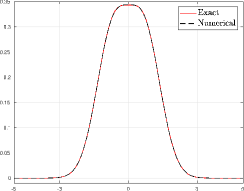
(a) Initial MDF $g(0,v_{1})$

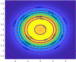
(b) Contours of $h(0,v_{1},v_{2})$

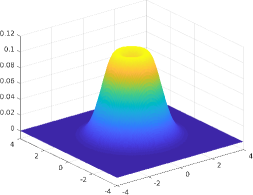
(c) Initial MDF $h(0,v_{1},v_{2})$

Figure 1: Figure (a) is the initial marginal distribution functions $g(0,v_{1})$. The red solid line corresponds to the exact solution, and the blue dashed line corresponds to the numerical approximation. Figure (b) is the initial marginal distribution functions $h(0,v_{1},v_{2})$. The blue solid lines correspond to the exact solution, and the red dashed lines correspond to the numerical approximation. Figure (c) shows only the numerical approximation.

Numerical results for $t=0.01$, $0.02$ and $0.06$ are given in Figures 2 and 3, respectively for the marginal distribution function $g(t,v_{1})$ and $h(t,v_{1},v_{2})$. Here we set $M_{0}$ as $M_{0}=5$ and $15$. For $M_{0}=5$, the numerical solution provides a reasonable approximation, but still with noticeable deviations, while for $M_{0}=15$, the two solutions match perfectly in all cases.

(a) $t=0.01$

(b) $t=0.02$

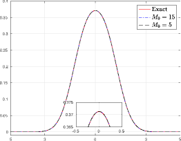
(c) $t=0.06$

Figure 2: Marginal distribution functions $g(t,v_{1})$ for $M_{0}=5$ and $15$ at $t=0.01$, $0.02$ and $0.06$. The red solid lines correspond to the exact solution, and the blue dot dashed and black dashed lines correspond to the numerical solutions with $M_{0}=15$ and $5$ respectively.

(a) $t=0.01,M_{0}=5$

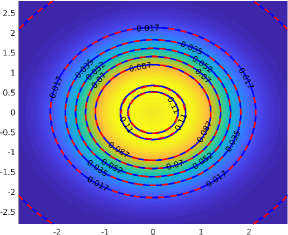
(b) $t=0.02,M_{0}=5$

(c) $t=0.06,M_{0}=5$

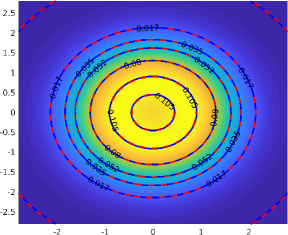
(d) $t=0.01,M_{0}=15$

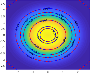
(e) $t=0.02,M_{0}=15$

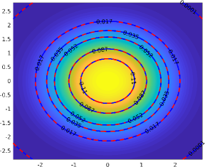
(f) $t=0.06,M_{0}=15$

Figure 3: Marginal distribution functions $h(t,v_{1},v_{2})$ for $M_{0}=5$ and $15$ at $t=0.01$, $0.02$ and $0.06$. The red dashed lines correspond to the exact solution, and the blue solid lines at different columns correspond to the numerical solutions $M_{0}=5$ and $M_{0}=15$.

Now we consider the time evolution of the expansion coefficients. By expanding the exact solution into Hermite series, we get the exact solution for the coefficients:

$$f_{\alpha}(t)=\left\{\begin{array}[]{ll}\left[-0.2\exp\left(-4t\right)\right]^{\frac{|\alpha|}{2}}\dfrac{1-|\alpha|/2}{(\alpha_{1}/2)!(\alpha_{2}/2)!(\alpha_{3}/2)!},&\text{if }\alpha_{1},\alpha_{2},\alpha_{3}\text{ are even},\\[13.0pt] 0,&\text{ otherwise}.\end{array}\right.$$ (5.1)

From (5.1), we can find that the coefficients $f_{\alpha}$ are zero for any $t$ if $1\leqslant|\alpha|\leqslant 3$. Hence we will focus on the coefficients $f_{400}$ and $f_{220}$ here. Figure 4 gives the comparison between the numerical solution and the exact solution for these two coefficients. In both plots, all the three lines coincide perfectly.

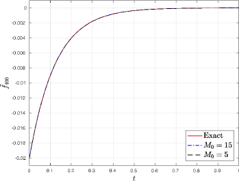
(a) $f_{400}(t)$

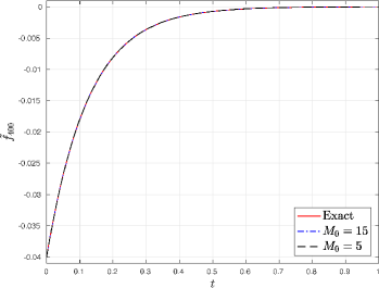
(b) $f_{220}(t)$

Figure 4: The evolution of the coefficients. The red lines correspond to the reference solution, and the blue dot dashed and black dashed lines correspond to the numerical solutions of $M_{0}=15$ and $M_{0}=5$ respectively.

5.2 Bi-Gaussian initial data

In this example, we perform the numerical test for the Bi-Gaussian problem. Here the Coulombian case $\gamma=-3$ are tested. The initial distribution function is

$$f(0,\boldsymbol{v})=\frac{1}{2\pi^{3/2}}\left[\exp\Big{(}-(v_{1}+\sqrt{3/2})^{2}+v_{2}^{2}+v_{3}^{2}\Big{)}+\exp\Big{(}-(v_{1}-\sqrt{3/2})^{2}+v_{2}^{2}+v_{3}^{2}\Big{)}\right].$$

In this numerical test, we use $M=20$ which gives a good approximation of the initial distribution function (see Figure 5).

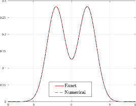
(a) Initial MDF $g(0,v_{1})$

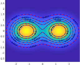
(b) Contours of $h(0,v_{1},v_{2})$

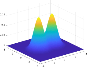
(c) Initial MDF $h(0,v_{1},v_{2})$

Figure 5: Figure (a) is the initial marginal distribution functions $g(0,v_{1})$. The red solid line corresponds to the exact solution, and the blue dashed line corresponds to the numerical approximation. Figure (b) is the initial marginal distribution functions $h(0,v_{1},v_{2})$. The blue solid lines correspond to the exact solution, and the red dashed lines correspond to the numerical approximation. Figure (c) shows only the numerical approximation.

For this example, we consider the three cases $M_{0}=5,10,15$, and the corresponding one-dimensional marginal distribution functions at $t=0.4$, $1$ and $3$ are given in Figure 6. In all the results, the numerical results are converging to the reference solution as $M_{0}=15$, and the lines for $M_{0}=10$ and $M_{0}=15$ are very close to each other. To get a clearer picture, similar comparisons of two-dimensional results are also provided in Figure 7.

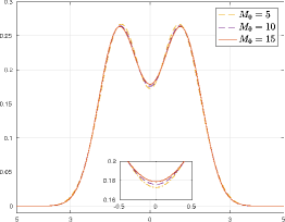
(a) $t=0.4$

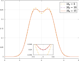
(b) $t=1$

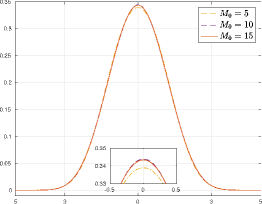
(c) $t=3$

Figure 6: The Coulombian case $\gamma=-3$. Marginal distribution functions at different times.

(a) $t=0.4,M_{0}=5$

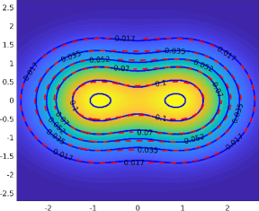
(b) $t=1,M_{0}=5$

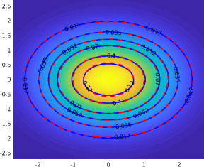
(c) $t=3,M_{0}=5$

(d) $t=0.4,M_{0}=10$

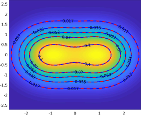
(e) $t=1,M_{0}=10$

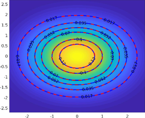
(f) $t=3,M_{0}=10$

Figure 7: The Coulombian case $\gamma=-3$. Comparison of numerical results with the reference solution. The red dashed contours are the reference solution as $M_{0}=15$. The blue solid contours at different columns are respectively the results for $M_{0}=5$ and $M_{0}=10$.

Now we consider the evolution of stress tensor and heat flux. In this example, we always have $\sigma_{11}=-2\sigma_{22}=-2\sigma_{33}$ and $q_{i}=0,i=1,2,3$. Therefore we focus only on the evolution of $\sigma_{11}$, which is plotted in Figure 8. It can be seen that even for $M_{0}=5$, the evolution of the stress tensor is almost exact, where the distribution function is not approximated very well. The three lines are all on top of each other.

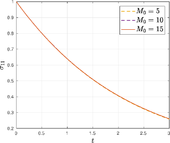
Figure 8: The Coulombian case $\gamma=-3$. Evolution of $\sigma_{11}(t)$. Three lines are on top of each other.

In order to test the computational capacity of our new model, the same example with a very small $\gamma$ as $\gamma=-4.9$ is tested. Here we also set $M=20$, and choose the numerical results with $M_{0}=15$ as the reference solution. Figure 9 shows the marginal distribution $h(t,v_{1},v_{2})$ at $t=0.4,1$ and $3$ with $M_{0}=5$ and $10$. It illustrates that when $\gamma$ equals $-4.9$, the numerical solutions are converging to the reference solution as $M_{0}=15$, and that the solution with $M_{0}=10$ is almost the same as the reference solution. The time evolution of $\sigma_{11}$ is plotted in Figure 10, where the three results are also on top of each other, even with $M_{0}=5$. Moreover, from Figure 9 and 10, we can find that the time evolution of the distribution function with $\gamma=-4.9$ is slower than that with $\gamma=-3$, which is also consistent with the form of the FPL collision operator.

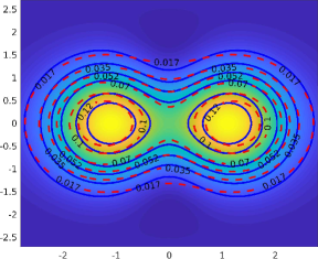
(a) $t=0.4,M_{0}=5$

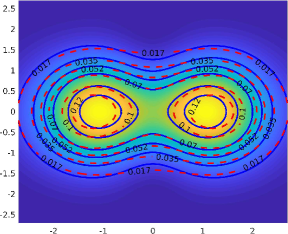
(b) $t=1,M_{0}=5$

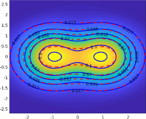
(c) $t=3,M_{0}=5$

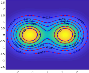
(d) $t=0.4,M_{0}=10$

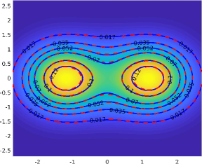
(e) $t=1,M_{0}=10$

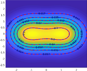
(f) $t=3,M_{0}=10$

Figure 9: The case $\gamma=-4.9$. Comparison of numerical solutions and the reference solution. The red dashed contours are the reference solutions $M_{0}=15$. The blue solid contours at different columns are respectively the numerical solutions $M_{0}=5$ and $M_{0}=10$.

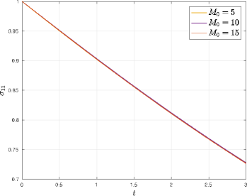
Figure 10: The case $\gamma=-4.9$. Evolution of $\sigma_{11}(t)$. Three lines are on top of each other.

5.3 Rosenbluth problem

In this example, the Rosenbluth problem is tested. Also the Coulombian case $\gamma=-3$ and the case $\gamma=-4.9$ are tested. The initial condition is from [25] as

$$f(0,\boldsymbol{v})=A\exp(-(B|\boldsymbol{v}|-1)^{2}).$$ (5.2)

The parameter $A,B$ are standardized to satisfy the condition that the initial density and temperature all equal $1$, precisely

$$A=\frac{(b/3)^{3/2}}{a^{5/2}},\qquad B=\frac{(b/3)^{1/2}}{a^{1/2}},$$ (5.3)

where $a=\pi(3\sqrt{\pi}({\rm erf}(1)+1+2/e)$ and $b=\pi(9.5\sqrt{\pi}({\rm erf}(1)+1)+7/e)$. Here $e$ is the Euler number and $\rm erf(x)=\frac{1}{\sqrt{\pi}}\int_{0}^{x}e^{-t^{2}}\,\mathrm{d}t$ is the error function.

In order to approximate the initial distribution function well, in this numerical test, we set $M=40$. The initial MDFs are plotted in Figure 11, which illustrates the perfect numerical approximation to the exact distribution function.

For this example, also the three cases $M_{0}=5,10,15$ are tested. The numerical solution with $M_{0}=15$ is treated as the reference solution. The corresponding one and two dimensional marginal distribution functions for the Coulombian $\gamma=-3$ are shown in Figure 12 and 13, where the numerical solutions are converging to the reference solution and that with $M_{0}=10$ is almost the same as the reference solution.

Moreover, our new model can also approximate the $\gamma=-4.9$ case well. The two dimensional marginal distribution functions for $\gamma=-4.9$ are presented in Figure 14. The numerical solution with $M_{0}=15$ is also chosen as the reference solution. Similar to the example in Sec 5.2, the time evolution of the distribution function with $\gamma=-4.9$ is also slower than that with $\gamma=-3$. Further more, though there are distinct differences between the numerical solution $M_{0}=5$ and $M_{0}=15$, the numerical solutions are converging to the reference solutions $M_{0}=15$.

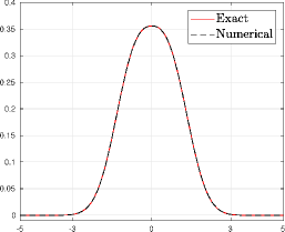
(a) Initial MDF $g(0,v_{1})$

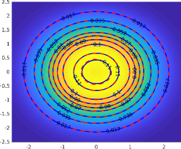
(b) Contours of $h(0,v_{1},v_{2})$

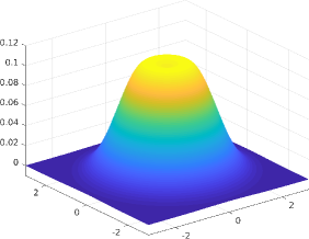
(c) Initial MDF $h(0,v_{1},v_{2})$

Figure 11: Figure (a) is the initial marginal distribution function $g(0,v_{1})$. The red solid line corresponds to the exact solution, and the blue dashed line corresponds to the numerical approximation. Figure (b) is the initial marginal distribution functions $h(0,v_{1},v_{2})$. The blue solid lines correspond to the exact solution, and the red dashed lines correspond to the numerical approximation. Figure (c) shows only the numerical approximation.

(a) $t=0.4$

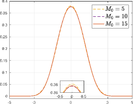
(b) $t=0.6$

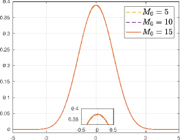
(c) $t=2$

Figure 12: The Coulombian case $\gamma=-3$. Marginal distribution functions at different times.

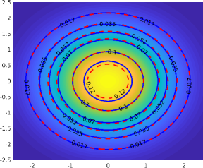
(a) $t=0.4,M_{0}=5$

(b) $t=0.6,M_{0}=5$

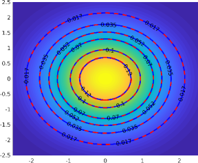
(c) $t=2,M_{0}=5$

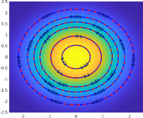
(d) $t=0.4,M_{0}=10$

(e) $t=0.6,M_{0}=10$

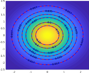
(f) $t=2,M_{0}=10$

Figure 13: The Coulombian case $\gamma=-3$. Comparison of numerical solutions and the reference solution $M_{0}=15$. The red dashed contours are the reference solution. The blue solid contours in different columns are respectively the numerical solutions $M_{0}=5$ and $M_{0}=10$.

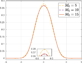
(a) $t=0.4$

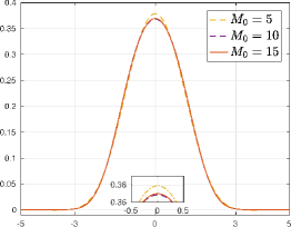
(b) $t=0.6$

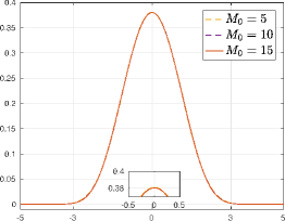
(c) $t=2$

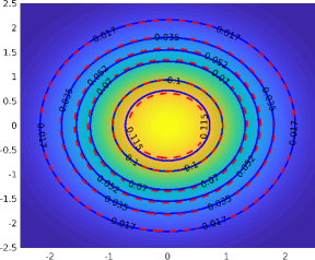
(d) $t=0.4,M_{0}=5$

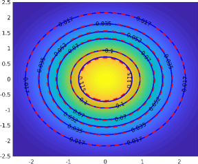
(e) $t=0.6,M_{0}=5$

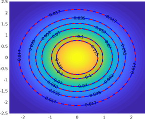
(f) $t=2,M_{0}=5$

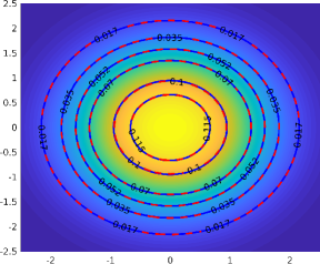
(g) $t=0.4,M_{0}=10$

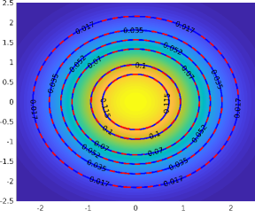
(h) $t=0.6,M_{0}=10$

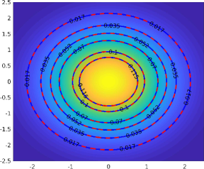
(i) $t=2,M_{0}=10$

Figure 14: The Coulombian case $\gamma=-4.9$. Marginal distribution functions at different times. The first row is the marginal distribution $g(t,v_{1})$, and the latter two rows are the marginal distribution functions $h(t,v_{1},v_{2})$ with different $M_{0}$. The red dashed contours are the reference solutions $M_{0}=15$. The blue solid contours at different rows are respectively the numerical solutions when $M_{0}=5$ and $M_{0}=10$.

6 Conclusion

In this paper, we focus on applying the Hermite spectral method to develop an efficient and accurate way of approximating and numerically solving the Fokker-Planck-Landau equation. Basic properties of Hermite polynomials are utilized to obtain a simplified expression of the coefficients, which renders the numerical method feasible. Burnett polynomials are introduced to deal with the super singular integral in the computation. This method could cover more practical cases up to $\gamma>-5$.

A novel collision model is built with a combination of quadratic collision model and the linearized collision model brought up by C. Villani [34]. The numerical experiments validate the efficiency of this new model. With the model introduced, the numerical solutions are of a high accuracy, as well as an affordable computational cost. This method should be further validated in the numerical tests for the full FPL equation with spatial variables, which will be one of the future works.

7 Appendix

7.1 Proof of Theorem 1

We shall present of proof of Theorem 1 here. In order to prove Theorem 1, we first introduce the lemma below:

Lemma 5.

Let $\boldsymbol{v}=\boldsymbol{h}+\boldsymbol{g}/2$ and $\boldsymbol{w}=\boldsymbol{h}-\boldsymbol{g}/2$. It holds that

$$\begin{split}&H^{\alpha}(\boldsymbol{v})H^{\kappa}(\boldsymbol{w})=\sum_{\alpha^{\prime}+\kappa^{\prime}=\alpha+\kappa}a_{\alpha^{\prime}\kappa^{\prime}}^{\alpha\kappa}H^{\alpha^{\prime}}(\sqrt{2}\boldsymbol{h})H^{\kappa^{\prime}}\left(\frac{\boldsymbol{g}}{\sqrt{2}}\right),\end{split}$$

where the coefficients $a_{\alpha^{\prime}\kappa^{\prime}}^{\alpha\kappa}$ are defined in (3.7).

Corollary 1.

Let $\boldsymbol{v}=\boldsymbol{h}+\boldsymbol{g}/2$. We have

$$H^{\alpha}(\boldsymbol{v})=\sum_{\kappa+\lambda=\alpha}\frac{2^{-|\alpha|/2}\alpha!}{\kappa!\lambda!}H^{\kappa}\left(\sqrt{2}\boldsymbol{h}\right)H^{\lambda}\left(\frac{\boldsymbol{g}}{\sqrt{2}}\right).$$

The proof of Lemma 5 can be found in [35]. Next we will prove Theorem 1.

Proof of Theorem 1.

Using an integration by parts and the recursion formula of Hermite polynomials

$$\frac{\partial}{\partial v_{s}}\Big{(}\mathcal{M}(\boldsymbol{v})H^{\alpha}(\boldsymbol{v})\Big{)}=(-1)\mathcal{M}(\boldsymbol{v})H^{\alpha+e_{s}}(\boldsymbol{v}),\qquad s=1,2,3,$$ (7.1)

the coefficients $A_{\alpha}^{\lambda,\kappa}$ (3.4) can be simplified as

$$A_{\alpha}^{\lambda,\kappa}=\sum_{s,t=1}^{3} \frac{\Lambda}{(\alpha-e_{s})!}\int_{\mathbb{R}^{3}\times\mathbb{R}^{3}}\lvert\boldsymbol{v}-\boldsymbol{v}^{*}\rvert^{\gamma}G_{st}(\boldsymbol{v}-\boldsymbol{v}^{*})$$ (7.2)

$$H^{\alpha-e_{s}}(\boldsymbol{v}^{*})\mathcal{M}(\boldsymbol{v})\mathcal{M}(\boldsymbol{v}^{*})\left(H^{\lambda}(\boldsymbol{v}^{\ast})H^{\kappa+e_{t}}(\boldsymbol{v})-H^{\lambda}(\boldsymbol{v})H^{\kappa+e_{t}}(\boldsymbol{v}^{*})\right)\,\mathrm{d}\boldsymbol{v}\,\mathrm{d}\boldsymbol{v}^{\ast},$$

where $G_{st}(\boldsymbol{v})=-v_{s}v_{t}+\delta_{st}|\boldsymbol{v}|^{2}$. Further simplification of (7.2) follows the method in [35], where the velocity of the mass center is defined as $\boldsymbol{h}=(\boldsymbol{v}+\boldsymbol{v}^{\ast})/2$ and the relative velocity is defined as $\boldsymbol{g}=\boldsymbol{v}-\boldsymbol{v}^{\ast}$. Hence, it holds that

$$\boldsymbol{v}=\boldsymbol{h}+\frac{1}{2}\boldsymbol{g},\quad\boldsymbol{v}^{\ast}=\boldsymbol{h}-\frac{1}{2}\boldsymbol{g},\quad|\boldsymbol{v}|^{2}+|\boldsymbol{v}^{\ast}|^{2}=\frac{1}{2}|\boldsymbol{g}|^{2}+2|\boldsymbol{h}|^{2},\qquad\mathrm{d}\boldsymbol{v}\,\mathrm{d}\boldsymbol{v}^{\ast}=\mathrm{d}\boldsymbol{g}\,\mathrm{d}\boldsymbol{h}.$$ (7.3)

Combing Lemma 5, (7.2) and (7.3), the integral in $A_{\alpha}^{\lambda,\kappa}$ can be rewritten with respect to $\boldsymbol{g}$ and $\boldsymbol{h}$

$$A_{\alpha}^{\lambda,\kappa}=2^{(\gamma/2+3-|\alpha|)/2}\sum_{s,t=1}^{3}\sum_{p+q=k-e_{s}}\sum_{r+\beta=\lambda+\kappa}\int_{\mathbb{R}^{3}\times\mathbb{R}^{3}}\lvert\boldsymbol{g}\rvert^{\gamma}\frac{\Lambda}{p!q!}G_{st}(\boldsymbol{g})H^{q}(\boldsymbol{g})\mathcal{M}(\boldsymbol{g})\mathcal{M}(\boldsymbol{h})$$ (7.4)

$$\left(a_{(\beta+e_{t})r}^{(\kappa+e_{t})\lambda}H^{r}(\boldsymbol{g})H^{\beta+e_{t}}(\boldsymbol{h})H^{p}(\boldsymbol{h})-a_{r(\beta+e_{t})}^{\lambda(\kappa+e_{t})}H^{\beta+e_{t}}(\boldsymbol{g})H^{r}(\boldsymbol{h})H^{p}(\boldsymbol{h})\right)\,\mathrm{d}\boldsymbol{g}\,\mathrm{d}\boldsymbol{h}.$$

Using the orthogonality of Hermite polynomials, we can finally prove Theorem 1.

∎

7.2 Proof of Theorem 4

In order to prove Theorem 4, we will introduce the lemma below:

Lemma 6.

For three spherical harmonics $Y_{l}^{m}$, $Y_{l_{1}}^{m_{1}}$ and $Y_{l_{2}}^{m_{2}}$, if $m\neq m_{1}+m_{2}$, or $l\not\in[|l_{1}-l_{2}|,l_{1}+l_{2}]$, then

$$\int_{\mathbb{S}^{2}}Y_{l_{1}}^{m_{1}}({\boldsymbol{n}})Y_{l_{2}}^{m_{2}}({\boldsymbol{n}})\overline{Y_{l}^{m}({\boldsymbol{n}})}\,\mathrm{d}{\boldsymbol{n}}=0.$$ (7.5)

Especially, we have

$$Y_{l}^{m}({\boldsymbol{n}})Y_{1}^{\mu}(\boldsymbol{n})=\sqrt{\frac{3}{4\pi}}\left(\eta_{l+1,m}^{\mu}Y_{l+1}^{m+\mu}({\boldsymbol{n}})+(-1)^{\mu}\eta_{-l,m}^{\mu}Y_{l-1}^{m+\mu}({\boldsymbol{n}})\right),\qquad\mu=-1,0,1,$$ (7.6)

where $\eta_{lm}^{\mu}$ is defined in (3.18).

The result of this lemma can be found in Section 12.9 of [1].

Proof of Theorem 4.

Noting that

$$n_{1}=\sqrt{\frac{2\pi}{3}}\left(Y_{1}^{1}-Y_{1}^{-1}\right),\qquad n_{2}=-\mathrm{i}\sqrt{\frac{2\pi}{3}}\left(Y_{1}^{1}+Y_{1}^{-1}\right),\qquad n_{3}=2\sqrt{\frac{\pi}{3}}Y_{1}^{0}.$$ (7.7)

Based on Lemma 6 and the property of spherical harmonic $\overline{Y_{l}^{m}(\boldsymbol{n})}=(-1)^{m}Y_{l}^{-m}(\boldsymbol{n})$, we can derive the results in Theorem 4 with the orthogonality property of spherical harmonics

$$\int_{\mathbb{S}^{2}}Y_{l_{1}}^{m_{1}}(\boldsymbol{n})\overline{Y_{l_{2}}^{m_{2}}({\boldsymbol{n}})}\,\mathrm{d}{\boldsymbol{n}}=\delta_{l_{1}l_{2}}\delta_{m_{1}m_{2}}.$$ (7.8)

∎

7.3 Computation of Coefficients $C_{\hat{{\alpha}}}^{{\alpha}}$

In this section, we will briefly introduce the algorithm to calculate $C_{\hat{{\alpha}}}^{{\alpha}}$, and the original algorithm is in [10].

Define

$$S_{-1}=\frac{1}{2}(v_{1}-\mathrm{i}v_{2}),\quad S_{0}=v_{3},\quad S_{1}=-\frac{1}{2}(v_{1}+\mathrm{i}v_{2}),$$ (7.9)

and the recursive formula of the basis functions [11] is

$$S_{\mu}B_{\hat{{\alpha}}}(\boldsymbol{v})=\frac{1}{2^{|\mu|/2}}\left[\sqrt{2(\hat{\alpha}_{1}+\hat{\alpha}_{3})+3}\eta_{\hat{\alpha}_{1}+1,m}^{\mu}B_{\hat{{\alpha}}+(1,\mu,0)^{T}}(\boldsymbol{v})-\sqrt{2\hat{\alpha}_{3}}\eta_{\hat{\alpha}_{1}+1,\hat{\alpha}_{2}}^{\mu}B_{\hat{{\alpha}}+(1,\mu,-1)^{T}}(\boldsymbol{v})\right.$$ (7.10)

$$\left.+(-1)^{\mu}\sqrt{2(\hat{\alpha}_{3}+\hat{\alpha}_{1})+1}\eta_{-\hat{\alpha}_{1},\hat{\alpha}_{2}}^{\mu}B_{\hat{{\alpha}}+(-1,\mu,0)^{T}}(\boldsymbol{v})-(-1)^{\mu}\sqrt{2(\hat{\alpha}_{3}+1)}\eta_{-\hat{\alpha}_{1},\hat{\alpha}_{2}}^{\mu}B_{\hat{{\alpha}}+(-1,\mu,1)^{T}}(\boldsymbol{v})\right],$$

where $\eta_{lm}^{\mu}$ is defined in (3.9) and we set $B_{\hat{{\alpha}}}(\boldsymbol{v})=0$ if $|\hat{\alpha}_{2}|>\hat{\alpha}_{1}$ or either of $\hat{\alpha}_{1},\hat{\alpha}_{3}$ is negative. Based on the recursion formula of Hermite polynomials

$$v_{s}H^{{\alpha}}(\boldsymbol{v})=H^{{\alpha}+e_{s}}(\boldsymbol{v})+k_{s}H^{{\alpha}-e_{s}}(\boldsymbol{v}),\qquad s=1,2,3,$$ (7.11)

we can get the recursive formula to compute $C_{\hat{{\alpha}}}^{{\alpha}}$, precisely

$$a_{\hat{{\alpha}}+e_{2}}^{(-1)}C_{\hat{{\alpha}}+e_{1}}^{{\alpha}}+b_{\hat{{\alpha}}+e_{2}}^{(-1)}C_{\hat{{\alpha}}-e_{1}+e_{3}}^{{\alpha}} =\frac{1}{2}k_{1}C_{\hat{{\alpha}}+e_{2}}^{{\alpha}-e_{1}}-\frac{\mathrm{i}}{2}k_{2}C_{\hat{{\alpha}}+e_{2}}^{{\alpha}-e_{2}},$$ (7.12)

$$a_{\hat{{\alpha}}}^{(0)}C_{\hat{{\alpha}}+e_{1}}^{{\alpha}}+b_{\hat{{\alpha}}}^{(0)}C_{\hat{{\alpha}}-e_{1}+e_{3}}^{{\alpha}} =k_{3}C_{\hat{{\alpha}}}^{{\alpha}-e_{3}},$$

$$a_{\hat{{\alpha}}-e_{2}}^{(1)}C_{\hat{{\alpha}}+e_{1}}^{{\alpha}}+b_{\hat{{\alpha}}-e_{2}}^{(1)}C_{\hat{{\alpha}}-e_{1}+e_{3}}^{{\alpha}} =-\frac{1}{2}k_{1}C_{\hat{{\alpha}}-e_{2}}^{{\alpha}-e_{1}}-\frac{\mathrm{i}}{2}k_{2}C_{\hat{{\alpha}}-e_{2}}^{{\alpha}-e_{2}},$$

where $|{\alpha}|=|\hat{{\alpha}}|_{B}$ and

$$a_{\hat{{\alpha}}}^{(\mu)}=\frac{1}{2^{|\mu|/2}}\sqrt{(2(\hat{\alpha}_{1}+\hat{\alpha}_{3})+3)}\eta_{\hat{\alpha}_{1}+1,\hat{\alpha}_{3}}^{\mu},\quad b_{\hat{{\alpha}}}^{(\mu)}=\frac{(-1)^{\mu+1}}{2^{|\mu|/2}}\sqrt{2(\hat{\alpha}_{3}+1)}\eta_{-\hat{\alpha}_{1},\hat{\alpha}_{3}}^{\mu},\quad\mu=-1,0,1,$$ (7.13)

As is stated in [10], we solve all the coefficients $C_{\hat{{\alpha}}}^{{\alpha}}$ by the order of $|{\alpha}|$, so that the right-hand sides of (7.12) are always known. The initial condition and the boundary conditions are $C_{\boldsymbol{0}}^{\boldsymbol{0}}=1$ and $C_{\hat{{\alpha}}}^{{\alpha}}=0$ if $|\hat{\alpha}_{2}|>\hat{\alpha}_{1}$ or either of $\hat{\alpha}_{1},\hat{\alpha}_{3}$ is negative. Moreover, the time complexity for computing all the coefficients $C_{\hat{{\alpha}}}^{{\alpha}}$ with $|\hat{{\alpha}}|_{B}=|{\alpha}|\leqslant M$ is $O(M^{5})$.

References

• [1] G. Arfken and H. Weber. Mathematical Methods for Physicists, Sixth Edition. Academic Press, 2005.
• [2] A. Arsen’ev and O. Buryak. On the connection between a solution of the Boltzmann equation and a solution of the Landau-Fokker-Planck equation. Math. USSR Sbornik, 69(2):465, 1991.
• [3] Yu. Berezin, V. Khudick, and M. Pekker. Conservative finite-difference schemes for the Fokker-Planck equation not violating the law of an increasing entropy. J. Comput. Phys., 69(1):163–174, 1987.
• [4] G. Bird. Molecular Gas Dynamics and the Direct Simulation of Gas Flows. Oxford: Clarendon Press, 1994.
• [5] A. Bobylev and I. Potapenko. Monte carlo methods and their analysis for coulomb collisions in multicomponent plasma. J. Comput. Phys., 246:123–144, 2013.
• [6] C. Buet and S. Cordier. Conservative and entropy decaying numerical scheme for the isotropic Fokker-Planck-Landau equation. J. Comput. Phys., 145(1):1228–245, 1998.
• [7] C. Buet and S. Cordier. Numerical analysis of conservative and entropy schemes for the Fokker-Planck-Landau equation. SIAM J. Numer. Anal., 36(3):953–973, 1999.
• [8] C. Buet, S. Cordier, and F. Filbet. Comparison of numerical schemes for Fokker-Planck-Landau equation. ESAIM: Proc., 10:161–181, 2001.
• [9] D. Burnett. The distribution of molecular velocities and the mean motion in a non-uniform gas. Proc. London Math. Soc., 40(1):382–435, 1936.
• [10] Z. Cai, Y. Fan, and Y. Wang. Burnett spectral method for the spatially homogeneous Boltzmann equation. arXiv:1810.07804, 2018.
• [11] Z. Cai and M. Torrilhon. Numerical simulation of microflows using moment methods with linearized collision operator. J. Sci. Comput., 74(1):336–374, 2018.
• [12] P. Degond and B. Lucquin-Desreux. The Fokker-Planck asymptotics of the Boltzmann collision operator in the coulomb case. Math. Models Methods Appl. Sci., 02(02):167–182, 1992.
• [13] P. Degond and B. Lucquin-Desreux. An entropy scheme for the Fokker-Planck collision operator of plasma kinetic throey. Numer. Math., 68:239–262, 1994.
• [14] L. Desvillettes. On asymptotics of the Boltzmann equation when the collisions become grazing. Transport. Theor. Stat., 21(3):259–276, 1992.
• [15] G. Dimarco, R. Caflish, and L. Pareschi. Direct simulation Monte Carlo schemes for Coulomb interactions in plasma. Commun. Appl. Ind. Math, 1:72–91, 2010.
• [16] F. Filbet and L. Pareschi. A numerical method for the accurate solution of the Fokker-Planck-Landau equation in the nonhomogeneous case. J. Comput. Phys., 179(1):1–26, 2002.
• [17] J. Fok, B. Guo, and T. Tang. Combined hermite spectral-finite difference method for the Fokker-Planck equation. Math. Comp., 71:1497–1528, 2002.
• [18] I. Gamba and S. Rjasanow. Galerkin-Petrov approach for the Boltzmann equation. J. Comput. Phys., 366:341–365, 2018.
• [19] H. Grad. On the kinetic theory of rarefied gases. Comm. Pure Appl. Math., 2(4):331–407, 1949.
• [20] E. Ikenberry and C. Truesdell. On the pressures and the flux of energy in a gas according to Maxwell’s kinetic theory I. J. Rat. Mech. Anal., 5(1):1–54, 1956.
• [21] S. Jin and B. Yan. A class of asymptotic-preserving schemes for the Fokker-Planck-Landau equation. J. Comput. Phys., 230:6420–6437, 2011.
• [22] L. Landau. The transport equation in the case of coulomb interactions. In D. Haar, editor, Collected Papers of L. Landau, pages 163 – 170. Pergamon, 1965.
• [23] M. Lemou. Multipole expansions for the Fokker-Planck-Landau operator. Numer. Math., 78(4):597–618, Feb 1998.
• [24] M. Lemou and L. Mieussens. Implicit schemes for the Fokker-Planck-Landau equation. SIAM J. Sci. Comput., 27(3):809–830, 2005.
• [25] L. Pareschi, G. Russo, and G. Toscani. Fast spectral methods for the Fokker-Planck-Landau collision operator. J. Comput. Phys., 165(1):216–236, 2000.
• [26] M. Pekker and V. Khudik. Conservative difference scheme for the Fokker-Planck equation. USSR. Comput. Maths. Math. Phys., 24(3):206–210, 1984.
• [27] D. Pfefferlé, E. Hirvijoki, and M. Lingam. Exact collisional moments for plasma fluid theories. Phys. Plasmas, 24(4):042118, 2017.
• [28] I. Potapenko and C. de Azevedo. The completely conservative difference schemes for the nonlinear Landau-Fokker-Planck equation. J. Comput. Appl. Math., 103(1):115–123, 1999. Applied and Computational Topics in Partial Differential Equations.
• [29] M. Rosenbluth, W. MacDonald, and D. Judd. Fokker-Planck Equation for an Inverse-Square Force. Phys. Rev., 107:1–6, 1957.
• [30] H. Srivastava, H. Mavromatis, and R. Alassar. Remarks on some associated Laguerre integral results. Appl. Math. Lett., 16(7):1131–1136, 2003.
• [31] W. Taitano, L. Chacón, A. Simakov, and K. Molvig. A mass, momentum, and energy conserving, fully implicit, scalable algorithm for the multi-dimensional, multi-species Rosenbluth-Fokker-Planck equation. J. Comput. Phys., 297:357–380, 2015.
• [32] C. Villain. A review of mathematical topics in collisional kinetic theory. In S. Friedlander and D. Serre, editors, Handbook of Mathematical Fluid Dynamics, volume 1, pages 71–305. North Holland, 2002.
• [33] C. Villani. On a new class of weak solutions to the spatially homogeneous Boltzmann and Landau equations. Arch. Rat. Mech. Anal., 143(3):273–307, 1998.
• [34] C. Villani. On the spatially homogeneous Landau equation for Maxwellian molecule. Math. Models Methods Appl. Sci., 08(06):957–983, 1998.
• [35] Y. Wang and Z. Cai. Approximation of the Boltzmann collision operator based on Hermite spectral method. arXiv:1803.11191, 2018.
• [36] C. Zhang and M. Gamba. Deterministic conservative solver for the inhomogeneous Fokker-Planck-Landau equation coupled with poisson equation. AIP Conf. Proc., 1786(1):180008, 2016.
• [37] D. Zhang, G. Wei, D. Kouri, and D. Hoffman. Numerical method for the nonlinear Fokker-Planck equation. Phys. Rev. E, 56:1197–1206, Jul 1997.