The Most Luminous Supernovae

Abstract

Over a decade ago, a group of supernova explosions with peak luminosities far exceeding (often by $>100$) those of normal events, has been identified. These superluminous supernovae (SLSNe) have been a focus of intensive study. I review the accumulated observations and discuss the implications for the physics of these extreme explosions. $\bullet$ SLSNe can be classified into hydrogen poor (SLSNe-I) and hydrogen rich (SLSNe-II) events. $\bullet$ Combining photometric and spectroscopic analysis of samples of nearby SLSNe-I and lower-luminosity events, a threshold of M${}_{g}<-19.8$ mag at peak appears to separate SLSNe-I from the normal population. $\bullet$ SLSN-I light curves can be quite complex, presenting both early bumps and late post-peak undulations. $\bullet$ SLSNe-I spectroscopically evolve from an early hot photospheric phase with a blue continuum and weak absorption lines, through a cool phtospheric phase resembling spectra of SNe Ic, and into the late nebular phase. $\bullet$ SLSNe-II are not nearly as well studied, lacking information based on large sample studies. Proposed models for the SLSN power source are challenged to explain all the observations. SLSNe arise from massive progenitors, with some events associated with very massive stars (M$>40$ M_⊙). Host galaxies of SLSNe in the nearby universe tend to have low mass and sub-solar metallicity. SLSNe are rare, with rates $<100$ times lower than ordinary SNe. SLSN cosmology and their use as beacons to study the high-redshift universe offer exciting future prospects.

1 INTRODUCTION: A BRIEF HISTORICAL REVIEW

The luminosity of supernovae (SNe) was the defining feature of these remarkable stellar events, and set these apart from less luminous and much more common stellar eruptions such as classical novae. Observed SN populations are invariably dominated by Type Ia events, the most luminous of all common SNe (e.g., Gal-Yam et al. 2013). Analyzing the statistics of peak SN luminosities, Richardson et al. (2002) noted a population of rare, overluminous events that are significantly more luminous than SNe Ia (L$>1.2\times 10^{43}$ erg s^-1; M$<$-19.5). Following the discovery and detailed studies of a few nearby superluminous events (and in particular SN 2005ap, Quimby et al. 2007; SN 2006gy, Ofek et al. 2007, Smith et al. 2007; and SN 2007bi, Gal-Yam et al. 2009) this population become a focus of intense study. In particular, Quimby et al. (2011) used observations across a range of redshift in order to unify several fragmented reports and define a spectroscopic class of hydrogen-poor super-luminous events. Gal-Yam (2012) reviewed extant observation, provided a detailed historical review, set a fiducial threshold to consider an event as a superluminous supernova (SLSN), and introduced the subclasses of hydrogen poor (SLSN-I) and hydrogen-rich (SLSN-II) events. More recently, this class of objects was reviewed by Howell (2017) and by Gal-Yam (2017) in the context of supernova classification, while Moriya et al. (2018) provide a broad theoretical perspective. The goal of this review is to update and expand on the work of Gal-Yam (2012), using a substantially larger data set collected since: 98 SLSNe are currently listed on WISeREP (Yaron & Gal-Yam, 2012), a sample $>5$ times larger than the 18 events available for analysis in 2012.

2 DEFINING THE CLASS OF SUPERLUMINOUS SUPERNOVAE

2.1 Luminosity Threshold

SLSNe are by definition more luminous than normal events (see Gal-Yam 2017 for a summary of the properties of normal SN classes), with individual events as luminous as L_bolometric$>3\times 10^{44}$ erg s^-1 (Vreeswijk et al., 2014). Gal-Yam (2012) set an arbitrary fiducial luminosity threshold of absolute magnitude L$>7\times 10^{43}$ erg s^-1 (M$<$-21 mag) in any band to consider object as superluminous. The drawbacks of this choice (beyond its arbitrary nature) are obvious, and include ambiguity due to choice of observing bands, color effects and K-corrections, that are significant for SLSNe at high redshifts. Additional ambiguity involves the event timescale. In this review, we focus on events that maintain their peak luminosity over a minimal time scale of $>48$ hours. This excludes shorter, luminous flares that can reach $>10^{44}$ erg s^-1, such as those associated with supernova explosion shocks (e.g., Yaron et al. 2017) and Gamma-Ray Burst afterglow emission that is associated with some SNe Ic-BL. We also exclude events with a peak luminosity that is within the range of standard events, but that are exceptionally long-lived such that they can reach a high integrated luminosity over several years (e.g., Miller et al. 2010; Ben-Ami et al. 2014; Arcavi et al. 2017).

[] Transient sky surveys providing samples of SLSNe: PTFThe Palomar Transient Factory; Law et al. (2009) PS1-MDSThe PanSTARRS1 Medium Deep Survey (PS1 MDS); Chambers et al. (2016) TSSThe Texas Supernova Survey (TSS); Quimby et al. (2013) SNLSThe Supernova Legacy Survey (SNLS); Prajs et al. (2017)

De Cia et al. (2018) inspected a large sample of Type I (hydrogen poor) SLSNe, as well as normal and broad-line (BL) SNe Ic from PTF in order to test whether a natural luminosity threshold emerges from the data (e.g., a double peaked luminosity distribution of normal and superluminous events). However, after correcting for the much larger volume probed by the PTF survey for SLSNe, the luminosity distributions of SLSNe-I, SNe Ic and SNe Ic-BL seem to join smoothly into a single distribution. Current observations therefore do not support a natural luminosity threshold separating SLSNe-I from lower-luminosity SNe Ic.

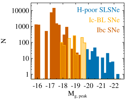
Figure 1: A histogram of the luminosity of SLSNe-I, SNe Ic and SNe-Ic-BL from PTF with a volumetric correction accounting for the detectability of more luminous events out to larger distances, adapted from De Cia et al. (2018) with perission from the AAS. The more luminous events (blue) also share spectral similarity according to Quimby et al. (2018) suggestion a threshold of M${}_{g}=-19.8$ mag may separate SLSNe-I from lower-luminosity events.

Inserra et al. (2018) conduct a more sophisticated analysis of the photometric properties of SLSNe-I and propose a set of 4 photometric parameters (the peak magnitude at restframe 400 nm, the magnitude decline in this band within 30 restframe days from peak, and the 400 nm - 520 nm color at peak and at 30 d after), that can be used to statistically select SLSNe-I without a luminosity threshold. While this method could be used to select SLSNe-I from large samples of events, it has several limitations: It does not apply to all SLSNe-I (for example, those with double-peaked light curves); it is only $90\%$ complete even within the restricted event sub-sample presented by Inserra et al. (2018), it requires multiband photometric coverage during and after peak, and its selection purity (number of false SLSN identifications) has not been robustly estimated. It thus cannot be used as a definition of the SLSN-I class at this time.

Similar analysis is yet to be carried out for hydrogen-rich SLSNe-II. While individual events exist that span the range ($>5$ mag) of luminosities from normal events to the most luminous SLSN-II, it is unclear whether the most luminous events are drawn from a luminosity distribution that smoothly extends to normal events.

2.2 Spectroscopic Definition

Lacking a clear luminosity threshold, one may hope to find a spectroscopic definition for SLSNe, i.e., a set of spectroscopic features that are common to SLSNe and differ from those of normal, lower-luminosity events. Quimby et al. (2018) were able to achieve this for the hydrogen poor (SLSN-I) variety. Applying an estimate for spectral similarity based on automated $\chi^{2}$ minimization ranking against spectral template libraries, these authors show that the most luminous events are also spectroscopically similar, and a threshold exists (M${}_{\rm g}=-19.8$ mag) that separates the more luminous events (blue in Fig.1) and more common events with normal luminosity. As this threshold separates presumably two distributions of different object clasees, one does not expect it to be sharp: rare luminous “normal” SNe may have brighter peak magnitudes, as there could be some spectroscopic SLSNe-I that fall below this threshold. Yet, at this time this value seems to offer a useful threshold. For example, the implied lower luminosity threshold for SLSNe-I includes all of the events spectroscopically identified by Lunnan et al. (2018) as SLSNe-I in their luminosity-unbiased analysis of events from the PS1-MDS survey.

At this time, no similar investigations have been conducted for SLSNe-II.

2.3 Relation to Normal Events

2.3.1 Hydrogen-poor SLSNe-I

Even though the volume-corrected luminosity distributions of SLSNe-I, SNe Ic and SNe Ic-BL join smoothly (De Cia et al. 2018; Fig.1), several differences exist between these populations suggesting that SLSNe are not just the upper luminosity tail of SNe Ic, as supported also by spectroscopic analysis (Quimby et al., 2018). De Cia et al. (2018) point out that the rise time of SLSNe-I is significantly longer compared to that of normal events with similar decay times, i.e., that the ratio of rise to decay time constitutes a photometric criterion to statistically separate these populations. In addition, as discussed below, early bumps prior to the first peak appear to be common in SLSNe-I (Nicholl & Smartt, 2016) and are very rare in less luminous SNe Ic. Finally, Perley et al. (2016) and Schulze et al. (2018) show that the fraction of SLSNe-I from all SNe is strongly suppressed in typically high-mass galaxies with metallicity above Z=0.4-0.5Z_⊙, unlike normal SNe Ic (but perhaps similar to SNe Ic-BL, e.g. Arcavi et al. 2010; Kelly & Kirshner 2012).

2.3.2 Hydrogen-rich SLSNe-II

Due to very few studies, it is hard to determine whether and how SLSNe-II are related to lower-luminosity SNe II. Host galaxy properties do seem to suggest a distinction between SLSNe-II and lower luminosity SNe ($\S$ 8).

[h]

3 A photometric threshold for hydregen-poor superluminous supernovae (SLSN-I)

The combination of photometric and spectroscopic analysis of the PTF sample of SLSN-I (De Cia et al. 2018; Quimby et al. 2018) suggests an absolute magnitude threshold of M${}_{g}=-19.8$ mag, above which all H- and He-poor events in this sample belong to a single spectroscopic similarity class that we identify as SLSN-I.  

4 CLASSIFICATION OF SUPERLUMINOUS SUPERNOVAE

The classification scheme of SLSNe follows that of lower-luminosity events (Gal-Yam, 2017) and relies mainly on near-peak flux visible-light spectroscopy.

4.1 SLSN-I

Fig.2 shows typical pre-peak spectra of this class of hydrogen-poor SLSNe. The strongest lines in visible-light spectra of SLSNe-I arise from the cumulative absorption of a large number of dense OII transitions in the blue (3000Å $<\lambda<$ 5000Å; see, e.g., Quimby et al. 2018). In the UV there are several strong absorption features, while the red part of the spectrum shows typically much weaker features of OI and CII (see, e.g., Gal-Yam 2018). At later phases, weeks to months after peak, the spectrum evolves and becomes similar to that of more normal SNe Ic around peak (Fig.3). Below we refer to these two phases as the hot and cool photospheric phases (see $\S$ 6.2.1 and $\S$ 6.2.2, respectively).

Spectroscopic classification of SLSNe-I is thus usually done at or before peak based on either the identification of the OII complex in low-redshift events, or the UV lines that are redshifted into the visible for higher-redshift SLSNe (Fig.2). Events lacking peak spectra can alternatively be classified by a combination of high peak luminosity and late-time similarity to SNe Ic (Fig. 3).

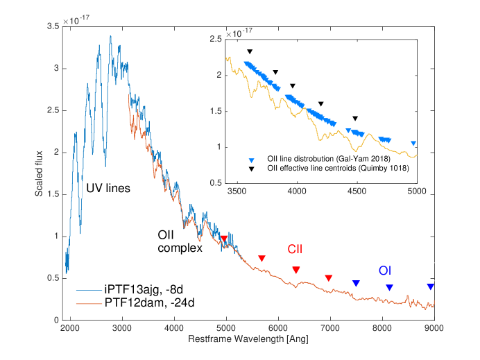
Figure 2: Pre-peak spectra of SLSNe-I during the hot photospheric phase ($\S$ 6.2.1). Combining visible-light observations of typical high-redshift (iPTF13ajg, z=0.74; Vreeswijk et al. 2014) and low-redshift (PTF12dam, z=0.1075; Quimby et al. 2018) events traces the near UV and optical spectrum covering the SLSN emission peak. Weak lines of OI and CII are detected redward of 5000Å. A dense forest of OII absorption features dominates the spectrum between 3500Å and 5000Å, with the strongest features appearing around 4200Å and 4500Å, and several strong absorption features are seen in the UV below 3200Å. Inset: an illustration of the formation of the OII complex by a dense distribution of OII lines. Gaps in the distribution of OII transitions (blue) appear as emission “peaks”. The effective central wavelengths of the five main OII absorption features calculated by Quimby et al. 2018 (4650.71Å, 4357.97Å, 4115.17Å, 3959.83Å, and 3737.59Å) are plotted in black and match the data very well. Lines of all elements have been shifted by an expansion velocity of 11000 km s^-1.

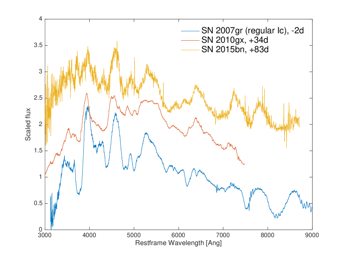
Figure 3: Post-peak spectra of SLSNe-I during the cool photospheric phase ($\S$ 6.2.2). Several weeks (e.g., SN 2010gx; Pastorello et al. 2010, Quimby et al. 2018) to months (e.g., SN 2015bn; Nicholl et al. 2016) after peak, SLSN-I evolve to resemble normal SNe Ic around peak (SN 2007gr shown for comparison; Valenti et al. 2008).

[8cm] Spectra shown in this and all other figures are publicly available from WISeREP (Yaron & Gal-Yam, 2012)

4.1.1 Proposed subdivisions

Gal-Yam (2012) proposed a possible division among hydrogen-poor SLSNe into rapidly declining SLSNe-I and slowly-declining events (with a decay rate consistent with radioactive decay of ⁵⁶Co) designated SLSN-R. This division was not broadly adopted. Recent sample studies (e.g., De Cia et al. 2018, Lunnan et al. 2018 and Nicholl et al. 2017) fail to find a clear natural division into two distinct classes of rapidly- and slowly-declining hydrogen-poor events (though Lunnan et al. 2018 may see a hint for bimodality).

Inserra et al. (2018) conduct a more sophisticated statistical analysis (including unsupervised clustering) of multiple photometric and spectroscopic parameters of SLSNe-I, and claim that a restricted set of events does cluster into two groups defined by rapid/slow evolution. This interesting work is limited by small numbers (only 3 events cluster into the slow category). Inserra et al. (2017) inspect the light curve properties of slowly-fading SLSNe-I, and propose that these may show ubiquitous post-peak undulations. Spectroscopic analaysis conducted by Quimby et al. (2018) also suggests a division based on similarity to two prototype events (PTF12dam and SN2011ke) that are slowly- and rapidly-declining SLSNe-I. A clear test of whether distinct groups of SLSN-I exist would greatly benefit from the large numbers of events expected for forthcoming massive surveys. Until that time, the term SLSN-I is applied to the entire class.

4.2 SLSN-II

Hydrogen-rich SLSNe-II show clear spectroscopic signatures of hydrogen around peak. He features are often also seen, especially in early, hot events.

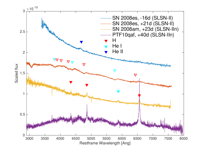
Figure 4: Spectra of SLSNe-II. SLSNe-IIn show strong H Balmer emission lines over a blue continuum at early time (SN 2008am; Chatzopoulos et al. 2011) evolving into a more complex spectrum after peak (PTF10qaf; Gal-Yam 2012). Rare SLSNe-II do not show narrow emission lines but rather blue continuum spectra (with broad He II in the case of SN 2008es shown; Gezari et al. 2009) that evolve into broad absorption features of H and He I after peak (Miller et al. 2009; empty markers have been blueshifted by 6000 km s^-1 to match the observed absorption features).

4.2.1 The Narrow-line SLSN-IIn class

The majority of events (similar in numbers to SLSNe-I; Gal-Yam 2012; Perley et al. 2016) show prominent emission lines of the hydrogen Balmer series, often accompanied by He I, with a narrow core over a broader base (Fig. 4), similar to lower luminosity SNe IIn. Initially some objects show a blue continuum with Balmer emission lines only, while more complex spectra develop later (Fig. 4).

4.2.2 The SLSN-II class and its relation to SLSN-I

The first hydrogen-rich SLSN that did not exhibit narrow Balmer lines was SN 2008es (Gezari et al. 2009; Miller et al. 2009; Fig. 4). The sample of similar events remains small and currently includes but a handful of additional events including CSS121015 (Benetti et al., 2014), SN 2013hx and PS15br (Inserra et al., 2018).

The group is characterized by spectra with evident Balmer lines in absorption or with P-Cygni profiles, but lacking narrow IIn-like features, an important distinction as such narrow features are generally taken as evidence for strong CSM interaction. Spectra are typically featureless initially with lines developing with time and becoming strong post-peak. Late spectra, in particular those studied by Benetti et al. (2014) evolve to strongly resemble late SLSN-I spectra superposed with a weak Balmer series, suggesting a connection between these rare SLSNe-II and the more common SLSNe-I, perhaps driven by a small amount of residual hydrogen left in the outer stellar envelope when these SNe explode.

PTF10hgi is currently a unique case of a SLSN that was initially classified as a SLSN-I, but actually shows clear spectral signatures of hydrogen and helium (Quimby et al., 2018), motivating a classification of SLSN-IIb in analogy to lower luminosity events. Interestingly, this event is also among the few that cannot be satisfactorily fit by a parameterized magnetar model by De Cia et al. (2018), and is an outlier in the analysis of Nicholl et al. (2015), having very slow photospheric velocities.

[h]

5 Summary of SLSN classification

Hydrogen-poor SLSNe-I lack strong features of hydrogen in peak-light spectra. Hydrogen-rich events include SLSNe-IIn that show strong narrow emission lines of hydrogen, SLSNe-II that show broad hydrogen absorption features, and a single SLSN-IIb that shows strong absorption features of both H and He.  

6 OBSERVED PROPERTIES OF SLSNE

6.1 Photometry

As a class, SLSNe of both types I and II typically have longer timescales in both rise and fall from peak compared to most lower luminosity events. Fig 5 shows the bolometric light curve of PTF12dam from Vreeswijk et al. (2017). This slowly-declining SLSN-I was discovered shortly after explosions and extensively followed.

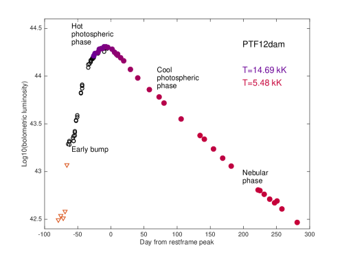
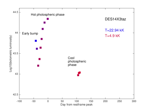
Figure 5: Top: the bolometric light curve of PTF12dam, a well-observed slowly-declining SLSN-I from Vreeswijk et al. (2017). The symbols are color-coded based on the temperature fits from Vreeswijk et al. (2017); values prior to -25 d require extrapolations and are less certain, and not coded. Main spectroscopic phases discussed below are marked for reference. PTF12dam transitioned from the hot to the cool photospheric phase about a month after peak, and went into the nebular phase around 200 d post-peak. An early bump is detected shortly after explosion (Vreeswijk et al., 2017). Late (post-peak) bumps, often seen in slowly-declining events (Inserra et al., 2017) are not obvious in the bolometric light curve of this event. Bottom: A similar plot for the rapidly-declining SLSN-I DES14X3taz from Smith et al. (2016). This event has a prominent early bump, during which the temperature measured is significantly hotter than at peak. The decline from peak to the cool photospheric phase is rapid but not well measured; for such rapid decliners, nebular phase observations are challenging.

6.1.1 SLSNe-I

6.1.1.1 Typical light curves: peak

As explained in $\S$ 2.1, when correcting for the larger volume within which more luminous events can be observed, SLSNe-I do not seem to separate from normal SNe Ib/c into a bimodal luminosity distribution, but hydrogen-poor SNe brighter than M${}_{g}=-19.8$ mag appear to belong to the spectroscopic class of SLSNe-I (De Cia et al. 2018; Quimby et al. 2018). The range of peak magnitudes observed extends from this lower cutoff up to M${}_{g}=-22.5$ or so for the brightest events (e.g., Vreeswijk et al. 2014). The mean peak luminosity of observed SLSN-I samples somewhat depends on the survey properties. Using a relatively small sample based on TSS, Quimby et al. (2013) find a a typical peak magnitude of M${}_{\rm unfiltered}=-21.7\pm 0.4$ mag. Several literature compilation studies find similar values, including Nicholl & Smartt (2016) that derived M${}_{g}=-21.62\pm 0.59$ mag (assuming M${}_{griz}=$M${}_{g}-0.9$ mag) and Inserra et al. (2018) that measure M${}_{400nm}=-21.7\pm 0.5$ mag. Applying a volumetric correction, De Cia et al. (2018) find a mean g-band absolute peak magnitude of M${}_{g}=-21.14\pm 0.75$ mag for the PTF sample, while Lunnan et al. (2018) measure M${}_{400nm}=-21.1\pm 0.7$ mag from PS1. Transforming either observed or calculated restframe magnitude distributions into luminosities depends on assumptions regarding SLSN-I K-corrections, but typical luminosity values are $2.5\times 10^{43}-5\times 10^{44}$ erg s^-1 (De Cia et al. 2018, Lunnan et al. 2018).

Of note is ASASSN-15lh (SN 2015L; Dong et al. 2016) a transient with a peak magnitude that stands out above even the most luminous SLSNe-I (M$\sim$-23.5 mag). However, the association of this transient with the class of SLSNe-I has been challenged (Leloudas et al., 2016; Gal-Yam, 2018) and remains uncertain.

6.1.1.2 Typical light curves: rise times

Using the time difference between first detection and peak as a lower limit on the rise time, the SLSN-I samples of Lunnan et al. (2018) and De Cia et al. (2018) include events with a bolometric rise time ranging from $\sim 20$ to $>100$ restframe days, with PTF10nmn and PS1-14bj being examples of events with extremely long rise times from each sample, respectively. Even the fastest-rising events have longer bolometric rise times than those of normal hydrogen-poor type I SNe ($<20$ d; e.g., Prentice et al. 2016). Various quantitative measures of the rise time are provides in the literature. De Cia et al. (2018) tabulate the time to rise by 1 mag or from half flux to peak in restframe g band, while Nicholl et al. (2015) and Lunnan et al. (2018) tabulate the bolometric time to rise from 1/e below maximum to peak. Nicholl et al. (2017) provide bolometric rise times estimated from light curve models that are consistent with the values cited above.

6.1.1.3 Typical light curves: decay times and slopes

SLSN-I decay times are typically slower than those of normal SNe I (e.g., Nicholl et al. 2015, De Cia et al. 2018). Since SLSNe are rarely (if ever) followed till their physical disappearance (i.e., when the SN is less luminous than its progenitor star), absolute decay times are not well defined. Various works tabulate decay slopes, ranging in restframe g band from $<0.01$ to about 0.08 mag d^-1 (e.g., De Cia et al. 2018), or times to decay by 1 mag or to 1/2 of peak flux (De Cia et al., 2018) or by 1/e (Nicholl et al. 2015, Lunnan et al. 2018). Alternatively, measures of the light decay in a certain band in magnitudes within a given period in days (e.g., $\Delta$M₂₀, $\Delta$M₃₀) is measured, for example by Inserra & Smartt (2014) and Inserra et al. (2018).

6.1.1.4 Early bumps

Leloudas et al. (2016) identified an early $\sim 10$ d long bump in the rising light curve of the SLSN-I SN 2006oz. Additional examples were later identified including the well observed LSQ14bdq (Nicholl et al., 2015) and DES14X3taz (Smith et al., 2016). Vreeswijk et al. (2017) presented a weak bump that was evident in early observations of PTF12dam, as well as an extreme early bump in the light curve of iPTF13dcc. Early bumps for which color information exists indicate the emission is initially very hot ($\sim 25000$ K) and cools rapidly (Smith et al., 2016; Nicholl & Smartt, 2016, see Fig. 5). Bump durations range from about 10 d to several weeks, and bump luminosities extend from about -19 mag to above -21 mag for the extreme iPTF13dcc, making these bumps brighter than almost all normal supernovae and in some cases rivaling in flux and duration the main peak of SLSNe. Nicholl & Smartt (2016) undertook a systematic search for such early bumps in the light curves of a literature sample of SLSNe-I. They find evidence for plausible early bumps in 8 of the 14 events with relevant early data, and can not rule out the existence of such a bump in any of the events, suggesting that these bumps may be common or even ubiquitous in SLSNe-I. However, the recent, nearby SN 2018bsz seems to lack a distinct bump, showing instead a long, slowly-rising early plateau (Anderson et al., 2018); and the sample of SLSNe from the DES survey also shows that significant early bumps are not ubiquitous (C. Inserra, private communication).

6.1.1.5 Late bumps

SN 2007bi, one of the first published SLSNe-I (Gal-Yam et al., 2009), showed apparent minor undulations in its declining post-peak light curve. Nicholl et al. (2016) studied the well observed SN 2015bn, and documented several undulation occurring up to $\sim 100$ days post peak, with typical durations of $\sim 20$ d and amplitudes of $\sim 20\%$ compared to a smooth fit to the bolometric light curve. The bumps appeared to result from excess blue light. Inserra et al. (2017) inspected several slowly-declining SLSNe-I, and found evidence for such small late-time bumps in all the objects studied. Light curves of more rapidly-declining events lack similar evidence for multiple bumps, though a single rapidly-declining event may show a late-time bump (Nicholl et al., 2016; Inserra et al., 2017) and in any case the rapid fading of these events makes detection of weak features post-peak more difficult. Whether such late bumps are correlated with a slowly-declining light curve thus remains an open question.

6.1.2 SLSNe-II

The information about SLSNe-II is scarce compared to studies of SLSNe-I. Preliminary results from a sample study of PTF events (Leloudas et al., in preparation, private communication) indicate that the sample, which is dominated by SLSNe-IIn, has a mean peak magnitude of M${}_{r}=-21.1\pm 0.5$. Rise times are comparable to, and decay times are longer than, those measured for SLSNe-I from the same survey.

6.1.2.1 Precursors

Ofek et al. (2014) present the detection of a pre-explosion precursor eruption prior to the luminous Type IIn supernova PTF10weh (peak magnitude M${}_{g}=-20.7$ mag). It is not clear at this time whether there is a threshold separating SLSNe-IIn from lower-luminosity events, and if so, whether PTF10weh should be considered a SLSN-IIn. In any case, pre-explosion LBV-like massive eruptions could explain the evidence for massive CSM surrounding at least some SLSNe-IIn (see $\S~{}$7.1.4 below).

6.2 Spectroscopy: SLSNe-I

SLSNe-I evolve through three main phases in their spectral evolution.

6.2.1 Hot photospheric phase

Initially, SLSN spectra are dominated by a hot blue continuum, with black-body temperatures often reaching 20000 K before maximum light (e.g., Smith et al. 2016; Bose et al. 2018; Fig. 5). Absorption features are detected on top of the continuum, typically of OI and CII in the red part of the visible light spectrum (e.g., Gal-Yam 2018, Anderson et al. 2018), the OII absorption complex in the blue part of the visible spectrum (e.g., Quimby et al. 2018, Gal-Yam 2018) and several strong UV absorption features, see $\S$ 4.1, $\S$ 6.4 and Fig. 2 above.

The OII complex is quite unique to SLSNe-I, that are the only type of SNe where these features are detected persistently up to peak. As shown by Mazzali et al. (2016), the formation of these lines requires population of highly excited levels of OII, which in turn implies significant departure from LTE and high temperatures; these conditions probably do not persist in normal hydrogen-poor SNe. OII has a very large number of lines in the blue part of the visible light spectrum, all with comparable strength. Gal-Yam (2018) show that gaps in the distribution of these lines appear as emission “peaks” in the spectrum (Fig 2, inset). Quimby et al. (2018) synthesized the OII absorption spectrum based on line lists from NIST, and compared it to their data. They found some inconsistencies that might be due to a few specific poorly measured laboratory transition data, and after adjusting for these findings derive effective central wavelengths for the main absorption features that match the observations very well (Fig 2, inset).

The identification of the UV lines is less certain. As seen in Fig. 2, there are four absorption features in the near UV, approximately around 2680Å, 2450Å, 2200Å and 1950Å. Quimby et al. (2018) review the proposed identifications of these lines by several studies (Quimby et al., 2011; Dessart et al., 2012; Howell et al., 2013; Mazzali et al., 2016) that did not converge to a consensus. Adopting the identifications of Mazzali et al. (2016) whose models recover the spectral evolution of SLSNe-I across this and later phases, the reddest feature at 2680Å is due to MgII and CII, The next two arise from a combination of TiIII and CII, along with SiIII (2450Å) and CIII (2200Å) while the bluest feature at 1950Å is due to Fe III and Co III.

Typical expansion velocities derived from C and O lines before and around peak are v=$10000-15000$ km s^-1 (Quimby et al., 2018; Gal-Yam, 2018). The ejecta velocity dispersion $\Delta$v during this phase is remarkably narrow (Quimby et al., 2018; Gal-Yam, 2018) with lines from single transitions suggesting $\Delta$v=1500 km s^-1 (Gal-Yam, 2018), making SLSNe-I strong outliers to the correlation found by Modjaz et al. (2016) between expansion velocity (line blueshift) and velocity dispersion (line width) for SNe Ib/c (Gal-Yam, 2018).

Theoretical spectral synthesis studies of this phase have been conducted by Dessart et al. (2012), and more recently Mazzali et al. (2016) developed spectral synthesis models that reproduce the evolution of SLSNe-I through this and later stages.

6.2.2 Cool photospheric phase

As the photosphere expands and cools the spectrum of SLSNe-I evolves. In the visible, OII features weaken as the temperature falls below 12000 K or so (Bose et al., 2018; Mazzali et al., 2016), and the spectrum rapidly changes to resemble spectra of more normal SNe Ic once the temperatures are below 10000 K (Fig.3; Pastorello et al. 2010, Quimby et al. 2011). Mazzali et al. (2016) predict that He I lines should briefly appear during the transition phase. This transition typically occurs a few days to weeks after peak, though some events (in particular some slowly evolving events like SN 2015bn; Nicholl et al. 2016) cool to the transition temperature well before peak magnitude. Liu et al. (2017) conducted a thorough investigation of the spectroscopic evolution of SLSNe-I in comparison with SNe Ic. They find that in terms of expansion velocities deduced from Fe II lines that become observable as the SNe cool, SLSNe-I are more similar to SNe Ic-BL than to normal SNe Ic.

6.2.3 Nebular emission

As SNe continue to cool and expand, their ejecta eventually become transparent and they enter the nebular phase. This phase begins later in SLSNe ($>100$ d post-peak) compared to normal SNe Ic, indicating high density is maintained in the ejecta during a longer period, due to more massive ejecta, ionization effects, or a combination of these (e.g., Nicholl et al. 2015). Analysis of nebular spectra is a powerful probe of the physics of SNe, and it has been applied to SLSNe-I with suitable data over the years (e.g., Gal-Yam et al. 2009, Nicholl et al. 2016, Jerkstrand et al. 2017)

Nicholl et al. (2018) combine new nebular phase observations with a large literature sample (in particular the large PTF data set released by Quimby et al. 2018) of SLSN-I spectra to conduct a detailed analysis of the nebular emission from these events, based on line identifications from Inserra et al. (2017) and Jerkstrand et al. (2017). In order to account for the intrinsically different timescales of SLSNe, they normalize the spectral phase according to the respective light curves. These authors define an early nebular phase, beginning two exponential decay timescales after peak (a mean restframe phase of $\sim 180$ d after peak; equivalent to $\times 2.5$ the time to decline by 1 mag measured by De Cia et al. 2018), and a late nebular phase beginning after 4 exponential timescales ($\sim 360$ restframe days on average) after peak. Early nebular spectra contain residual continuum emission and the strongest emission line is often Ca II 7300Å, while late nebular spectra are typically dominated by the OI 6300Å line (Fig. 6).

Strong emission lines in high S/N mean spectra calculated by Nicholl et al. (2018) can be identified with ions of O, Mg, Ca, Fe and Na (Fig. 6). The spectra are overall similar to those of SNe Ic, but show stronger emission from Fe in the blue (as noted early on by Gal-Yam et al. 2009) suggesting a larger fraction of Fe-group elements in the ejecta. OI 7774Å is stronger in SLSNe compared to SNe Ic, and in some events OII and OIII lines are seen (Lunnan et al., 2014; Inserra et al., 2017), indicating high ionization. Nebular line widths are remarkably high, with FWHM velocities of OI 6300Å extending to above 15000 km s^-1 at the early nebular phase, and dropping to $\sim 8000$ km s^-1 during the late phase.

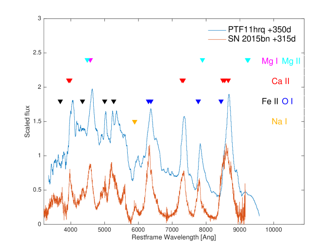
Figure 6: Nebular spectra of SLSNe-I. High S/N spectra of PTF11hrq from Quimby et al. (2018) and SN 2015bn from Jerkstrand et al. (2017) are shown; these are among the most nearby SLSNe-I with high quality late-time spectra. Line identifications are drawn from NIST; with the addition of the semi-forbidden line of Mg I at 4571Å.

6.2.4 Late-time emergence of hydrogen in SLSN-I

Yan et al. (2015) reported the first detection of an emerging emission of hydrogen in late-time spectra of the SLSN-I iPTF13ehe. Yan et al. (2017) presented two additional cases of such SLSNe-I with late-time hydrogen emission, and discussed the properties of this small sample. The first spectra of iPTF13ehe were obtained around peak, and the object was already in the cool photospheric phase; it resembled slowly-evolving events like SN 2007bi and SN 2015bn in both its light curve and its early spectra. About 250 d after peak, broad emission lines emerge, initially hydrogen H$\alpha$ and later (around 322 d after peak) also H$\beta$ and He I 5876Å become apparent. The two additional events presented by Yan et al. (2017) have narrower light curves, and their earlier spectra (obtained around peak) do not resemble the standard hot photospheric spectra of SLSNe-I described in $\S$ 6.2.1 (Gal-Yam, 2018), suggesting perhaps that SLSNe-I that present these late-time interaction features may also have distinct early spectra. The observations require a distribution of hydrogen-rich material lying at distances of a few$\times 10^{16}$ cm. Yan et al. (2015) estimate $\sim 15\%$ of SLSNe-I may show late-time hydrogen Balmer emission.

6.3 Spectroscopy: SLSNe-II

6.3.1 SLSNe-IIn

The spectroscopic evolution of samples of SLSNe-IIn has been poorly explored so far. Smith et al. (2008) and Smith et al. (2010) presented spectroscopic sequences extending to late phases of the luminous SLSNe-IIn SN 2006gy and SN 2006tf, respectively. Very roughly, the observations trace a spectral evolution beginning with blue spectra with a few emission lines with typically simple emission profiles, evolve into more complex spectra with significant structure in the continuum shape and emission line profiles, and eventually an evolution at late times (several hundred days) to spectra with very little continuum dominated by residual h$\alpha$ emission. There is significant variation among objects so that a more definitive description will have to wait for the publication of larger and better understood samples.

6.3.2 SLSNe-II

There are only a handful of events in this class of SLSNe-II without narrow lines (Gezari et al. 2009, Miller et al. 2009, Benetti et al. 2014, Inserra et al. 2018). However, their spectral evolution seems to be quite similar: initially the spectra show a hot blue continuum with weak or no features. This is followed (around 20 d or so after peak) by a significant cooling of the spectral continuum, along with development of more prominent lines, most notable a broad hydrogen H$\alpha$ that grows stronger for several months. As these events rapidly decline in flux, spectroscopic follow-up is usually limited in duration, but the few late-time spectra (Benetti et al., 2014; Inserra et al., 2018; Bhirombhakdi et al., 2018) show only H$\alpha$ emission at $>200$ d.

6.4 UV spectroscopy

The high UV luminosity of SLSNe made these objects attractive targets for UV spectroscopy using HST, extending to short wavelengths. Fig. 7 shows available spectroscopy down to 1000Å for SLSNe-I and SLSNe-II (Yan et al., 2017, 2018; Curtin et al., 2018).

Yan et al. (2018) compare the few available far UV spectra of SLSNe-I during the hot photospheric phase ($\S$ 6.2.1), and find these are quite homogeneous (Fig. 7). A significant fraction of the total luminosity of these events is emitted in the UV (e.g., $50\%$ below 2500Å for Gaia16apd, Yan et al. 2017) but that the optical-UV flux is not well described by a single BB function, and invoke varying degrees of additional UV flux suppression, perhaps reflecting the metal contents in the outer ejecta. Smith et al. (2018) collect a sample of high-redshift SLSNe-I with restframe UV spectra (redshifted into the visible) and provide further evidence that these objects have rather homogeneous spectra, peaking around 3000Å with varying UV suppression and marked diversity below 2500Å. They find no correlation between peak photometric magnitude and spectral properties, nor evidence for spectral evolution at least to modest ($z>1$) redshifts.

Far-UV Spectra of SLSNe-II are scarce. Fig. 7 shows the single HST spectrum available. This object shows weaker UV absorption features as well as Ly$\alpha$ emission supporting its classification as a SLSN-IIn. A larger sample of data is needed to further characterize the UV emission from this spectral class.

Figure 7: Far UV Spectra of SLSNe around peak. SLSNe-I (bottom curves) show a continuum with strong and wide absorption features. The wavelengths and equivalent width of these features are quite homogeneous among the few objects with available observations (Yan et al., 2018); a ground-based observation of iPTF13ajg (Vreeswijk et al., 2014) is also shown. The only far UV spectrum of a SLSN-IIn (LSQ15abl) has weaker features and some of these might be blended with host galaxy absorption features; however Ly$\alpha$ emission and CIV 1548Å absorption are broad and are therefore likely associated with the SN (Curtin et al., 2018).

6.5 Polarimetry

Only a handful of polarimetric studies of SLSNe-I were conducted so far (Leloudas et al., 2015; Inserra et al., 2016; Leloudas et al., 2017; Bose et al., 2018). An interesting result emerged from observations of SN 2015bn, that show a higher level of polarization after peak than prior to peak (Inserra et al., 2016; Leloudas et al., 2017), suggesting an ellipsoidal core (Inserra et al., 2016) within a more spherical envelope; consistent with analysis by Bose et al. (2018). The rapid increase in polarization degree that coincides with a sharp spectral transition (Fig 8; Leloudas et al., 2017) may suggest that the core/envelope border could mark the transition from a relatively pristine C/O progenitor envelope to an inner core of freshly synthesized heavier elements.

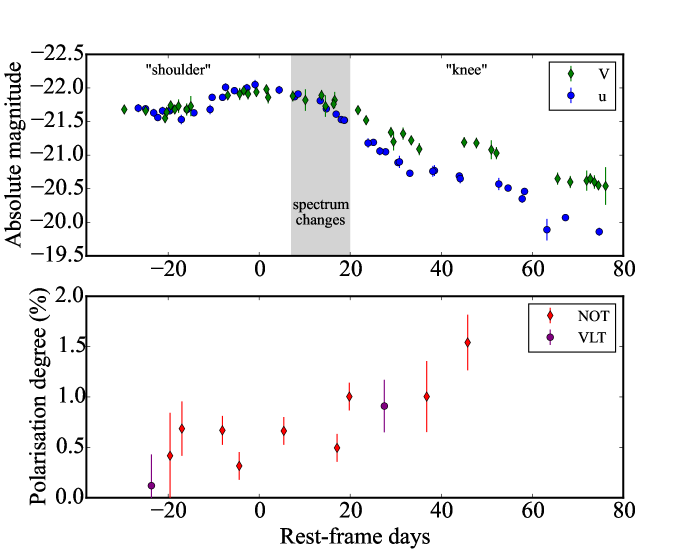
Figure 8: Time evolution of the polarisation of SN 2015bn (from Leloudas et al. 2017; reproduced with permission from the AAS) showing an increase in polarisation following the transition of this object from the hot to the cool photospheric phase.

6.6 Observations at other wavelengths

6.6.1 X-rays

X-ray observations of nearby SLSNe-I using Swift, Chandra, and XMM-Newton (Ofek et al., 2013; Levan et al., 2013; Margutti et al., 2017) have so far yielded null detections only. Ofek et al. (2013) report flux limit in the 0.2-10 keV band around peak magnitude extending from L${}_{\rm X}<0.5\times 10^{42}$ erg s^-1 for nearby ($z\approx 0.2$) events to about L${}_{\rm X}<2\times 10^{44}$ erg s^-1 for less well-observed or higher redshift events. Levan et al. (2013), Inserra et al. (2017) and Margutti et al. (2017) extend this work to a larger sample of events and later time, placing similar limits from pre-peak to $>1000$ d post-peak for some events. Margutti et al. (2017) also place much deeper limits (L${}_{\rm X}<2\times 10^{40}$ erg s^-1) on emission from PTF12dam prior to peak, interpreting the emission detected in the SN location in deep Chandra observations as arising from the vigorously star-forming host.

A remarkable exception is the distant (z=1.189) SLSN-I SCP06F6. Levan et al. (2013) use XMM observations obtained about 100 restframe days after discovery to measure L${}_{\rm X}\approx 10^{45}$ erg s^-1 in 0.2-2 keV X-rays, making SCP06F6 the most luminous X-ray supernova ever detected. Such an emission would have been easily detected for the tens of lower-redshift events monitored with Swift indicating that either this was an exceptional SLSN-I, or that X-ray emission from SLSNe-I is extremely short-lived and has been missed for most events and fortuitously observed for SCP06F6, or that perhaps the XMM detection is unrelated to the SLSN. Additional similar detections for other SLSNe-I may have significant implications for the physics of these events (Levan et al., 2013).

6.6.2 Radio

GHz radio observations of SLSNe-I have yielded only non-detections so far. Nicholl et al. (2016) report a deep VLA upper limit 238 d after maximum. Bose et al. (2018) report deep limits (L${}_{\rm 10GHz}<5.4\times 10^{26}$ erg s${}^{-1}\,Hz$^-1) at the location of the nearby SN2017egm observed around peak, the tightest limits placed so far. These limits rule out an association of these SLSNe-I with GRB-like engines, as even low-luminosity GRB radio afterglow emission would have been recovered (Bose et al., 2018). A radio luminosity similar to those of some regular SNe Ib/c is not ruled out.

7 PHYSICS OF SUPERLUMINOUS SUPERNOVAE

Reviewing all the theoretical aspects related to the physics of SLSNe lies far outside the scope of this review. We therefore focus on aspects of SLSN physics that can be related relatively directly to the observations reviewed above.

7.1 Energy Source - SLSNe I

A main puzzle about the nature of SLSNe-I is the energy source that powers these very luminous and often very long-lived events. Several possible mechanisms have been proposed and are briefly reviewed here. Sukhbold & Woosley (2016) review the maximal theoretical energy output of such models, and find that current observations are so far within the theoretically allowed range. A summary of the models strengths and weaknesses is presented in Table 1.

7.1.1 Central engines - magnetars

A rapidly spinning newborn megnetar was first invoked as an extra power source for a supernova by Maeda et al. (2007). This idea was further developed and applied to SLSNe by Woosley (2010) and Kasen & Bildsten (2010). A popular implementation of the model (Inserra et al., 2013) fits the observed light curves and constrains three physical parameters: the ejecta mass M_ej, the initial magnetic field B and the initial magnetar period P. Variants of this model have now been fit to large samples of SLSNe-I (e.g., Liu et al., 2017; Nicholl et al., 2017; De Cia et al., 2018). Nicholl et al. (2017) find typical derived values for the physical parameters are B$\approx 10^{14}$ G, P$\approx 2$ ms, and M${}_{\rm ej}\approx$5 M_⊙, with the mass estimate having a scatter of at least $\times 2$ with more massive ejecta typically found for the slowly-declining SLSNe-I; De Cia et al. (2018) find similar values for P and somewhat higher values for B. Overall, photometric observations of most SLSNe-I around peak magnitude are well fit by this model, though see De Cia et al. (2018) for a few exceptions.

Dessart et al. (2012) and Mazzali et al. (2016) calculate synthetic photospheric spectra of SLSNe-I using assumptions motivated by magnetar models and provide good fits to observed spectra. Jerkstrand et al. (2017) carry out similar successful modelling of nebular spectra of some slowly-declining SLSNe-I. Overall, magnetar-based models seem to be able to fit both the basic light curves and spectra of SLSNe-I.

The magnetar model does face some challenges though. As pointed out by Nicholl et al. (2015), the early bump seen in many SLSNe-I before peak ($\S$ 6.1.1.4), if interpreted in the context of standard shock-cooling models, requires a large explosion energy ($>10^{52}$ erg) that might be challenging for neutron-star forming magnetar models. However, Kasen et al. (2016) introduce the idea of magnetar shock breakout, that could explain these early bumps.

Another challenge for this model is that light curve models calculated to fit the early-time observations of SLSNe-I tend to over-predict the emission at late phases (e.g., Chen et al. 2015, Vreeswijk et al. 2017). To alleviate this discrepancy, it is often assumed that the ejecta become progressively transparent with time, such that the energy deposition from the slowing-down magnetar is not fully trapped at late epochs. Since the nature of the energy output from the magnetar engine and its interaction with the ejecta is unspecified, this may be equivalent to introducing a free time-dependent escape function, making comparison to observations less constraining for the model.

As the magnetar model predicts a smooth, monotonically decreasing energy generation, it cannot naturally explain the post-peak late bumps ($\S$ 6.1.1.5) observed in several SLSNe. Metzger et al. (2014) proposed that emerging ionization fronts can create such features, and Nicholl et al. (2016) suggest a similar idea based on oxygen recombination; however, Inserra et al. (2017) argue why both of these ideas are unlikely to explain the multiple undulations seen in some slowly-decaying SLSNe-I. Combined with strong evidence for late-time interaction seen in some objects (see below), these authors suggest magnetar-only models are insufficient and hybrid models (e.g., magnetar + interaction) may be required.

Finally, a consistency issue with this model manifesting as a “missing mass” problem appears to arise when comparing ejecta masses derived using the latest data compilation of Nicholl et al. (2017) with ejecta masses derived from extensive nebular spectroscopy modelling by Jerkstrand et al. (2017). For slowly declining SLSNe-I and in particular for SN 2007bi, the magnetar model light-curve-derived mass ($3.8$ M_⊙) is $>4$ times smaller than the lower limit from Jerkstrand et al. (2017) ($>15$ M_⊙) and inconsistent with previous estimates from Nicholl et al. (2015). However, see Nicholl et al. (2018) for a discussion of the caveats of such a comparison.

7.1.2 Central engines - BH accretion

Dexter & Kasen (2013) propose fallback accretion onto a newly formed black hole (BH) following the core-collapse of a massive star can power SN-like transients, including SLSNe of both type I and II. This model is similar in many respects to the magnetar model described above, having a central engine energizing the expanding SN ejecta, but unlike the magnetar model, no simple prescription connecting the observed light curve to the model physics exists, beyond the prediction that the late-time energy supply rate falls with time as $t^{-5/3}$.

While there are few direct comparisons of SLSN observations with predictions based on BH fallback accretion models (beyond those provided by Dexter & Kasen 2013), these models do have some potential benefits. In particular, unstable mass accretion onto the BH (as is often the case in, for example, AGN) can naturally explain light curve undulations on various timescales ($\S$ 6.1.1.5), and Kasen et al. (2016) claim that BH fallback accretion events can also drive a shock breakout flare that can explain the initial bumps observed ($\S$ 6.1.1.4).

With a large reservoir of fallback mass to draw from, and exploiting the high mass to energy conversion possible for thin accretion disks around BHs, the energy budget of BH accretion models is substantially larger than available for NS-forming models (including magnetar models), making them attractive for very energetic events, especially in terms of large integrated luminosity.

7.1.3 Radioactivity

Gradual energy injection by radioactive decay of newly synthesized radioactive nuclides (most notably ⁵⁶Ni) is generally assumed to be the power source of standard SNe I (both SNe Ia and SNe Ib/c). Some amount of ⁵⁶Ni is assumed to form in most variants of massive star explosion models. A particular theoretical variant, predicted to occur for extremely massive stellar cores, involves a rapid contraction of the core following loss of pressure due to electron-positron pair production, leading to a thermonuclear explosion that disrupts the star (Barkat et al., 1967; Rakavy & Shaviv, 1967). Such Pair-Instability SN (PISN) explosions are predicted to produce, for high-mass cores, very large amounts of ⁵⁶Ni (several solar masses) and therefore result in very luminous SNe (Kasen et al., 2011).

The intrinsic nature of ⁵⁶Ni radioactivity as an energy source relates the peak luminosity and integrated energy (both roughly proportional to the total ⁵⁶Ni mass) to the ejecta mass and opacity (since Ni and other Fe-group elements have high opacity). One would expect therefore high peak luminosity to be accompanied by long diffusion times for radiation in the ejecta, that should manifest as long rise times to peak. In addition, the energy production rate is known (for ⁵⁶Ni and its progeny, ⁵⁶Co, the predicted deline rate at late times is $\sim 0.01$ mag d^-1), up to an escape function that is also amenable to calculation, since the energy is deposited into the ejecta by $\gamma$-rays and positrons, and one can calculate the relevant transport equations. This makes radioactivity-based models highly predictive and testable. For PISNe in particular, large ⁵⁶Ni masses are produced (Heger & Woosley, 2002) from explosions of very massive cores, predicting ejected masses of order $\sim 100$ M_⊙, and SN rise times of $>100$ d (Kasen et al., 2011).

In the context of SLSNe-I, the discussion of radioactive models has initially forked into two channels. For some slowly-declining events, in particular for SN 2007bi (Gal-Yam et al., 2009), PISN models seemed to provide a good fit to available observations. For the group of more rapidly-declining SLSNe-I, radioactive models were disfavored (Quimby et al., 2011). This led Gal-Yam (2012) to propose that there are two separate groups of SLSNe-I, those powered by radioactivity (SLSNe-R) and those that are not (SLSNe-I). However, additional work challenged the association of slowly-declining SLSNe-I with PISNe (Nicholl et al., 2013). In particular, PISN spectroscopic models seem to disagree with observations for both the photospheric (Dessart et al., 2012) and nebular (Jerkstrand et al., 2017) phases. In addition, as detailed above, additional analysis does not clearly support a division of SLSNe-I into two separate subclasses based on their light curve shapes.

PISN models producing the large amounts of ⁵⁶Ni relevant for SLSNe-I require very massive exploding cores (with masses $\sim 100$ M_⊙, e.g., Gal-Yam et al. 2009; Kasen et al. 2011). Assuming a monotonic initial mass function extending to these extremely massive stars, the detection of even a handful of such objects implies there should be a much larger population of fainter PISN explosions (producing much less ⁵⁶Ni from slightly less massive cores; Heger & Woosley 2002). Kozyreva et al. (2018) present a plausible candidate for such an event, and the discovery and study of additional similar events by the new generation of massive all-sky transient surveys is an interesting prospect for the nearby future.

At this time, it seems like the radioactive (and in particular, PISN) model is relevant only for a very small subclass of SLSNe-I, that show both a very long rise time, and a slow decline - the two best examples are PS1-14bj (Lunnan et al., 2016) and PTF10nmn (Kozyreva & Blinnikov, 2015; De Cia et al., 2018). While observations of events with spectra similar to the models of Dessart et al. (2012) have not been published, alternative models (Kozyreva et al., 2017) seem to be, at least roughly, compatible with observations of some SLSNe-I, making the viability of PISN models more a theoretical than an observational debate.

7.1.4 CSM Interaction

Interaction with CSM around an exploding star is an efficient mechanism to convert the ejecta kinetic energy into radiation via strong shocks. Such a CSM (see Smith 2014 for a review) may result from thick stellar winds, binary interaction and mergers, or stellar eruptions (e.g., of LBV stars). A particular physical mechanism that is often mentioned is pulsational pair-instability (e.g., Woosley et al., 2007; Waldman, 2008; Woosley, 2017, and references therein), occurring when massive stellar cores become pair-unstable, but the resulting contraction is halted prior to full core disruption, leading to an ejection of a limited amount of mass - the process may repeat several times prior to final core-collapse.

CSM interaction is likely responsible for powering hydrogen rich type IIn SNe, helium-rich SNe Ibn, rare luminous SN Ia explosions (Ia-CSM) and even some SNe Ic (see Gal-Yam 2017 for a recent review of these SN classes). While most interacting SNe show strong emission lines, making this mechanism mostly relevant to SLSNe-II (see below), evidence for interaction with hydrogen-free material largely without prominent emission lines (e.g., Ben-Ami et al. 2014) motivates consideration of this powering mechanism also for SLSNe-I.

Several lines of evidence suggest CSM interaction may be important in powering at least some SLSNe-I. Late-time observations of some SLSNe show emerging emission lines of hydrogen (Yan et al., 2017, $\S$ 6.2.4) or other elements (Lunnan et al., 2018) suggesting CSM shells surround the progenitors of some SLSNe-I. Lunnan et al. (2018) show evidence that the PPISN mechanism may have been responsible for the SLSN-I iPTF16eh.

The observation of post-peak undulations in several slowly-declining SLSNe-I can also be explained by interaction of the expanding ejecta with a structured CSM distribution, leading Inserra et al. (2017) to propose that CSM interaction likely contributes to powering these events.

Chatzopoulos et al. (2012) provide a semi-analytic formula to simulate CSM-powered SN light curves, that has been fit to numerous observed SLSNe. While this model is simple and has a lot of freedom (since it depends on the physical properties of both the SN and the CSM) it typically provides fits to light curves that are as good as those provided by Magnetar models (e.g., Nicholl et al., 2016; Vreeswijk et al., 2017).

A major shortcoming of the CSM models is that there are currently no published models that fit observed SLSN-I spectra assuming pure CSM interaction power. Nicholl & Smartt (2016) point out that having ubiquitous early bumps with similar properties in SLSN-I light curves would be surprising for interaction-powered models, since shock breakout is expected to occur in widely varying locations within complex CSM. The observations of Vreeswijk et al. (2017) suggest early bumps may indeed be more diverse than initially thought, as do recent observations of SN 2018bsz (Anderson et al., 2018) and the set of SLSNe-I from DES (C. Inserra, private communication), so early bump properties are probably not a significant challenge for CSM models.

7.1.5 Hybrid models

Hybrid models combine two or more of the specific models discussed above. Such combinations are in some sense expected and perhaps inevitable - for example, megnetar-forming SN explosions may also synthesize some amount of ⁵⁶Ni, some late-time CSM interaction may be expected for many massive-star explosions, and so on. Some hybrid models combine a leading model to explain most of the SLSN emission, with a secondary model to explain specific features that are hard to reproduce with the main model - for example, Inserra et al. (2017) advocate CSM interaction on top of a central engine explosion to explain slowly-declining SLSNe-I and their ubiquitous light curve undulations, while Chen et al. (2017) invoke CSM interaction to explain evidence for an additional luminosity source near peak. The inherent additional parametric flexibility in hybrid models makes them philosophically weaker compared to any single model, but with accumulated observations, perhaps no single model can explain all data.

Table 1: SLSN-I energy source models

Model	Strengths	Challenges / Weaknesses
Magnetar	Good fits to observed light curves	Early bumps
	Models fit photospheric spectra	Late decay slope
	Models fit nebular spectra	Post-peak bumps
		Interaction signatures
		“Missing mass” problem
Black Hole	Naturally explain LC undulations	Rarely tested with observations
	Potentially large energy supply	Interaction signatures
Radioactivitya	Predictive models fit some events	Spectroscopic behavior debated
CSM Interaction	Interaction signatures in some events	Early bumps
	Late bumps	No predictive spectral models
Hybrid models	Can fit most observations	Hard to test

^aOnly for the most slowly-rising SLSNe-I;

7.2 Energy sources - SLSNe-II

Since most SLSN-II show signs of CSM interactions similar to those of lower luminosity SNe IIn, it is natural to assume that these events are powered by continued conversion of the SN ejecta kinetic energy into radiation by distributions of massive CSM. Some cases require large explosion kinetic energies or large CSM masses, or both (e.g., Smith et al. 2010), but no clear cases have been published where an energetic core-collapse explosion of a massive star embedded in a thick CSM cannot suffice. Lacking published samples of events, information about typical physical properties of SLSNe-II are not yet available.

7.3 Progenitor stars

The association of SLSNe of all types with star-forming hosts (see $\S$ 8 below) strongly suggest these are explosions of massive stars. Analysis of host galaxy samples suggests the progenitors of SLSNe-I have a strong preference for sub-solar metallicity ($<0.5$ solar; see $\S$ 8 below).

7.3.1 Evidence for massive-star progenitors

Assuming SLSNe are massive star explosions, it is interesting to consider whether they arise from the same mass range as lower-luminosity events (e.g., $8-17$ M_⊙ for common SNe II, Smartt 2015), or do they arise from even more massive stars, and whether SLSNe-I and SLSNe-II have similar mass progenitors.

7.3.1.1 Slowly-rising SLSNe-I

There is strong evidence that at least some SLSNe arise from extremely massive stars. While initial claims for very massive progenitors for SLSNe-I with the most extended light curves, based on association of some events with PISN models (Gal-Yam et al., 2009) have been challenged (see $\S$ 7.1.3), the combined evidence from multiple lines of evidence, including both light curve analysis (Nicholl et al., 2015; Lunnan et al., 2016) as well as nebular spectroscopy, suggests very massive progenitors for these events, with ejecta masses of $>20$ M_⊙ and derived initial masses M$>40$ M_⊙ (Jerkstrand et al., 2017).

7.3.1.2 PPISNe

Lunnan et al. (2018) present evidence, based on spectroscopic analysis of the evolution of transient emission lines, interpreted as echoes from a CSM shell, associating the SLSN-I iPTF16eh with PPISN models. These models can potentially explain the origin of the CSM shell, and indicate an extremely massive progenitor with initial mass $>100$ M_⊙.

7.3.1.3 SLSNe-IIn

For several SLSNe-IIn with long duration light curves, the long diffusion time and large integrated luminosity require both massive ejecta and a massive CSM shell. Taken together, these require very massive progenitors, perhaps similar to massive LBVs (e.g, Smith et al., 2010). An association with massive LBV-like stars would also explain possible precursor eruptions that may be associated with at least some SLSNe-IIn (see $\S$ 6.1.2.1; Ofek et al. 2014).

7.3.1.4 Host galaxy eviedence

Leloudas et al. (2015) and Schulze et al. (2018) present evidence from the association of SLSNe-I with extreme emission line galaxies (EELGs) suggestion very young ages, and therefore very high progenitor initial masses (M$>60$ M_⊙), with some slowly-evolving events (e.g., PTF12dam, Thöne et al. 2015) coming from even higher masses (M$\approx$120 M_⊙; see $\S$ 8 below).

7.3.2 Metallicity

As shown in $\S$ 9 below, there is strong evidence from host galaxy population studies that the progenitors of SLSNe-I have low metallicity compared to that of the average massive star population at relatively low redshift (i.e., to recover the observed distribution of host galaxy properties, one must assume a suppression of SLSN-I formation above a metallicity of Z$=0.5$ Z_⊙). The lower their natal metallicity, stars of a given initial mass undergo weaker mass loss during their evolution (Langer, 2012). Such stars would thus evolve to have pre-explosion cores that are both more massive and retain more angular momentum, all other parameters being equal. Stars with rapidly rotating core are natural candidates to form central engines such as magnetars ($\S$ 7.1.1) and accreting black holes ($\S$ 7.1.2). The positive correlation shown by Kushnir (2015) between progenitor luminosity, and hence progenitor mass, and the resulting amount of radioactive ⁵⁶Ni synthesized in the resulting explosion, if it extends to large Ni masses, also makes low-metallicity stars favored progenitors for Ni-powered SLSN models ($\S$ 7.1.3), and in particular for PISN models for slowly-declining SLSNe-I (Langer et al., 2007; Langer, 2012; Kozyreva et al., 2017).

7.3.3 Possible connection with Gamma-Ray Bursts

The association of both SLSNe-I and long-duration GRBs with dwarf, star-forming galaxies, begs the question of a possible connection between these energetic cosmic explosion classes. As discussed in $\S$ 8 below, while the host galaxies of SLSNe-I and long-duration GRBs show some similarities, they also show significant differences.

Greiner et al. (2015) show a possible association between an ultra-long GRB and a supernova that is similar to members of the SLSN-I class. The implications of this discovery are unclear though, as the GRB is a member of a rare, unusual subclass (ultra-long duration GRBs; Levan et al. 2014) and the associated supernova is somewhat fainter and has spectral peculiarities (it is UV-faint) compared to other SLSNe-I. In any case, limits from observations of nearby GRBs indicate that most GRBs cannot be associated with SLSN-I explosions - all detected SNe associated with GRBs are fainter than SLSNe-I.

8 HOST GALAXIES OF SUPERLUMINOUS SUPERNOVAE

8.1 Population Studies

Neill et al. (2011) carried our the first sample study of SLSN hosts, including 17 SLSNe-I and SLSNe-II. Based on the UV and r-band properties of this initial literature compilation, they found that SLSNe occur in blue star-forming galaxies, prefer galaxies with low mass and high specific star formation, and suggested that SLSNe occurrence in high-mass galaxies is suppressed due to high metallicity.

Additional studies followed using larger samples of SLSNe-I, extensive photometric observations from IR to UV as well as spectroscopy (Lunnan et al., 2014; Leloudas et al., 2015; Angus et al., 2016; Perley et al., 2016; Schulze et al., 2018). Typical mean properties of SLSN host galaxies are M$<10^{9}$ M_⊙, specific star formation rates of $\sim 2$ Gy^-1 and low metallicities of 0.5 solar or below, with some exceptions. High resolution HST imaging (Lunnan et al., 2015; Angus et al., 2016) suggested a dominant compact irregular morphology for these dwarf hosts.

Lunnan et al. (2014) suggested SLSNe-I and long-duration GRBs occur in similar host galaxies within the overall population of star-forming galaxies, but this result was not supported by later studies (Leloudas et al., 2015; Angus et al., 2016; Schulze et al., 2018).

Taken together, the most recent results suggest that SLSNe-I likely occur mostly in compact, dwarf irregular galaxies, often with extremely strong emission lines (EELGs; EW${}_{\rm OIII}>100$Å, Leloudas et al., 2015), with an effective metallicity suppression above $0.5$ solar (Perley et al., 2016; Chen et al., 2017; Schulze et al., 2018). The hosts of SLSNe-IIn are different (Leloudas et al., 2015), span a very wide range of luminosities, masses and metallicities (Angus et al., 2016), possibly with metallicity suppression above 0.8 solar (Schulze et al., 2018) (though see Perley et al. 2016) but are distinct from host galaxies of the general core-collapse SN population (Schulze et al., 2018), for example in the fraction of events exploding in very low luminosity galaxies (Angus et al., 2016).

8.2 Absorption Spectroscopy

The high UV luminosity of SLSNe-I makes them attractive targets to UV absorption line studies that probe the ISM in and around the host galaxies of these events. Ground-based studies of this sort can be carried out for events with redshift $z>0.5$ once important UV metal lines are redshifted below the atmospheric cutoff. Berger et al. (2012) demonstrated this for a high-redshift SLSN-I from PS1. Vreeswijk et al. (2014) carried out an absorption line analysis for the high-redshift PTF object iPTF13ajg. Comparing Mg line absorption strengths for a sample of SLSNe-I and long-duration GRBs, they show that also in this respect, SLSNe-I hosts are distinct from GRB host galaxies in having weaker absorptions.

9 RATES

Quimby et al. (2013) use observations from the TSS survey to estimate the rate of SLSNe at low redshifts ($z\approx 0.15$). For SLSNe-I, they find a rate of $35^{+84}_{-29}$ events Gpc^-3 y^-1 for a Hubble constant H$=71$ km s^-1 Mpc^-1, based on a single event. The TSS survey discovered 3 SLSNe-II (2 SLSNe-IIn and a single SLSN-II, SN 2008es). The combined rate derived by Quimby et al. (2013) from these events is $151^{+151}_{-82}$ events Gpc^-3 y^-1. Note however that while the small TSS sample includes a single SLSN-II (without narrow lines) out of the sample of three SLSNe-II in total, the fraction of such SLSNe-II in literature compilations is much smaller (of order 10%; e.g., Gal-Yam 2012).

As noted by Gal-Yam (2012), the rates of SLSNe-I at low redshift are substantially lower than the rates of SNe Ib/c (25800 events Gpc^-3 y^-1; Li et al. 2011) as well as from the rate of low-redshift long-duration GRBs ($380^{+620}_{-225}$ events Gpc^-3 y^-1, Guetta & Della Valle 2007). If verified by better statistics, the fact that SLSN-I rates fall below that of GRBs suggests that if these events arise from massive progenitors in similar galaxies, the initial mass range of SLSN-I progenitors should be higher than that of GRB progenitors.

Prajs et al. (2017) measured the rate of SLSNe-I at higher redshifts ($z\approx 1.1$) using observations by the SNLS survey, and find a rate of $91^{+76}_{-36}$ events Gpc^-3 y^-1. Combined with the measurement at low redshift, the SLSN-I rate appears to rise in a manner consistent with the evolution of the cosmic star formation rate. These authors also find that the SLSN-I rate is substantially below that of SNe Ib/c or long GRBs, but is consistent with the rare class of ultra-long GRBs.

Cooke et al. (2012) used the detection of two likely SLSNe (lacking spectral confirmation) at very high redshifts (z=2.04 and z=3.9) to estimate the high-redshift rate of SLSNe, finding a rate of $\approx 400$ events Gpc^-3 y^-1 with very large errors. If these events are related to lower-luminosity SLSNe-I, then this rate is marginally above that expected from scaling the measurement of Prajs et al. (2017) by the cosmic star formation rate, suggesting that the fraction of SLSN progenitors of the massive star population may have been larger in the past.

10 POSSIBLE USE IN COSMOLOGY

Assembling a sample of SLSNe-I from the literature and their own observations, Quimby et al. (2013) noted that the peak magnitude of SLSNe-I tends to cluster quite strongly around the mean value (M$=-21.7$ mag) and speculated that this class of objects may become useful distance estimators for cosmology.

Inserra & Smartt (2014) investigated this option further using a larger sample of relatively well-observed events, and suggested that correlations between the peak magnitude and the light curve shape, as well as color, could help standardize these objects as cosmological probes, perhaps competitive with SNe Ia. De Cia et al. (2018) attempted to conducted a similar analysis on their sample of SLSNe-I, but could not provide further support to this result. Inserra et al. (2018) inspected correlations among photometric parameters of SLSNe-I, suggesting these do support their division into two photometric subclasses (slowly- and rapidly-declining events), and that these correlations can further assist in cosmological use of these events.

11 FUTURE PROSPECTS AND OPEN QUESTIONS

The study of SLSNe is a young subject with less than a dozen years having passed since the publications of the first pioneering works. It is clear that significant additional work remains in order to observationally characterize these objects and to better understand their physics. I highlight here several important open questions and areas where additional important progress is likely.

A major open question highlighted in this work is the energy source powering these extremely luminous and long-lived events. Are all SLSNe-I powered by the same source or are there two, or more, sub-groups? Are some or all SLSNe-II similar to SLSNe-I in this sense? Is a central engine definitely required, and if so, is it a Magnetar, an accreting black hole, or perhaps both channels are at work? Have we ever observed the results of the PISN and PPISN mechanisms? These and additional question remain open, and continue to drive a wide and extensive observational effort.

Type II SLSNe are significantly less well studied compared to SLSNe-I, and in particular sample studies are missing. Leloudas et al. (in preparation, see $\S$ 6.1.2.1) should provide at least an initial characterization of SLSNe-IIn in the nearby Universe, but additional studies, in particular also at higher redshifts, are certainly called for.

With multiple transient surveys such as ASASSN, ATLAS, PS and ZTF monitoring almost the entire sky (both hemispheres, from ground and from space using Gaia) with typical cadence of a few days or less, long-lasting and luminous nearby SLSNe should be detected with high completeness, as demonstrated, e.g., with the discoveries of Gaia16apd (Nicholl et al., 2017; Yan et al., 2017; Kangas et al., 2017), SN 2017egm (Bose et al., 2018) and SN 2018bsz (Anderson et al., 2018). As more and more events are studied at lower and lower distances, new observational windows open to study these luminous events with diverse instrumentation. I am especially excited about the prospects to closely monitor a nearby SLSN-I in X-rays in order to test whether an X-ray burst similar to the one detected by Levan et al. (2013) can be recovered; such an event could provide strong support to central-engine models.

Moving to the other extreme, the high UV luminosity of SLSNe makes them perhaps the best targets for studies of transients at high redshift. Following the pioneering work of Cooke et al. (2012), several works have already highlighted the prospects for detecting SLSNe at very high redshift using, for example, LSST, as well as future space missions such as Euclid (Inserra et al., 2018) and WFIRST (Smith et al., 2018). Wang et al. (2017) show that JWST could conduct a powerful survey for extremely high-redshift transients, and that $z>10$ SLSNe-I could be detected by JWST in the NIR bands; in fact, SLSNe (if they occur at very high redshifts) may be the most luminous source of light in the early universe, easily outshining infant galaxies. SLSNe at high redshift could be a focus of attention in the coming decade not only for the massive star, supernova and time-domain astronomy community, but also for those interested in the first stars, the early universe and the first sources of ionizing radiation.

12 SUMMARY

This review attempts to summarize our knowledge about SLSNe accumulated mostly in the last decade or so, from an observational perspective. SLSNe are spectroscopically classified into hydrogen-poor SLSNe-I and hydrogen-rich SLSNe-II.

Hydrogen-poor SLSNe-I are quite well characterized. This class includes events with a peak magnitude above a threshold of M${}_{g}=-19.8$ mag or so, based on a combination of photometric and spectroscopic studies of low-redshift SLSN-I samples ($\S$ 2.1). The light curves evolve more slowly than those of lower-luminosity SNe Ib/c, with typical rise times $>20$ d and a decay time distribution that extends to very slowly-declining events (Fig. 5). Light curve bumps and undulations are observed both at early ($\S$ 6.1.1.4) and late, post-peak ($\S$ 6.1.1.5) phases.

SLSNe-I evolve through several spectroscopic phases. A initial hot photospheric phase, charaterised by a blue continuum with high black-body temperature ($>12$ kK) with absorption features mostly of carbon and oxygen in visible light (Fig. 2) and several strong UV features (Fig. 7), typically persists until peak magnitude or a few weeks later (Fig. 5). This is followed by a cool photospheric phase with spectra similar to those of SNe Ic (Fig. 3) that further evolve into the nebular phase (Fig. 6) $>150$ d after peak.

Hydrogen-rich SLSNe-II are not nearly as well studied. The majority of these events show strong narrow emission lines of hydrogen and are spectroscopically similar to lower-luminosity SNe IIn ($\S$ 4); it is not clear if there is a threshold separating the SLSN-IIn population from their more common low-luminosity cousins. The mean peak magnitude of this population is M${}_{r}\approx-21.1\pm 0.5$ mag, and its rise and decay times are long, even compared to SLSNe-I ($\S$ 6.1.2.1). A handful of rare SLSNe-II show broad (but not narrow) hydrogen features, and some spectral similarities to SLSNe-I ($\S$ 4.2.2). A single event (PTF10hgi) should likely be spectroscopically classified as a SLSN-IIb.

The energy source of SLSNe-I is still an open question, with viable models including central-engine models driven by a newborn rapidly-spinning magnetar or an accreting black hole, interaction with hydrogen-poor CSM, or, perhaps for the most slowly-evolving events, models powered by large amounts of radioactive ⁵⁶Ni ($\S$ 7.1). The energy source for SLSNe-II is even less well understood. It is clear that interaction with CSM plays a major role for most of these events, but whether the underlying explosion is similar to that of lower-luminosity events is not known. The progenitor stars of SLSNe are young, massive stars; there is evidence that at least some events have extremely massive progenitors (M$>40$ M_⊙; $\S$ 7.3).

The host galaxies of SLSNe-I are typically compact, irregular dwarf galaxies with low stellar mass and high star formation rate, and often also with very strong emission lines. SLSN-I production seems to be suppressed above a metallicity threshold of Z$=0.5$ Z_⊙ ($\S$ 8). The hosts of SLSNe-II span a wider range of masses, but are also distinct from the hosts of lower-luminosity events. The rates of SLSNe are still rather poorly measured due to small number statistics, however, these events are rare, with volumetric rates at least two orders of magnitude below those of normal core-collapse SNe; SLSNe-I are likely rarer also from long-duration GRBs ($\S$ 9).

SLSNe-I have been proposed as cosmological probes visible to high redshifts, and several papers investigate this possibility, though the results are not yet conclusive ($\S$ 10). With likely near-term prospects extending from detection of additional very nearby SLSNe to the most distant events ($\S$ 11), the prospects of this young field of study for additional rapid development appear bright.

DISCLOSURE STATEMENT

The authors are not aware of any affiliations, memberships, funding, or financial holdings that might be perceived as affecting the objectivity of this review.

References

- Anderson et al. (2018) Anderson, J. P., Pessi, P. J., Dessart, L., et al. 2018, arXiv:1806.10609
- Angus et al. (2016) Angus, C. R., Levan, A. J., Perley, D. A., et al. 2016, MNRAS, 458, 84
- Arcavi et al. (2010) Arcavi, I., Gal-Yam, A., Kasliwal, M. M., et al. 2010, ApJ, 721, 777
- Arcavi et al. (2017) Arcavi, I., Howell, D. A., Kasen, D., et al. 2017, Nature, 551, 210
- Barkat et al. (1967) Barkat, Z., Rakavy, G., & Sack, N. 1967, Physical Review Letters, 18, 379
- Ben-Ami et al. (2014) Ben-Ami, S., Gal-Yam, A., Mazzali, P. A., et al. 2014, ApJ, 785, 37
- Benetti et al. (2014) Benetti, S., Nicholl, M., Cappellaro, E., et al. 2014, MNRAS, 441, 289
- Berger et al. (2012) Berger, E., Chornock, R., Lunnan, R., et al. 2012, ApJ, 755, L29
- Bhirombhakdi et al. (2018) Bhirombhakdi, K., Chornock, R., Miller, A. A., et al. 2018, arXiv:1807.07859
- Bose et al. (2018) Bose, S., Dong, S., Pastorello, A., et al. 2018, ApJ, 853, 57
- Chambers et al. (2016) Chambers, K. C., Magnier, E. A., Metcalfe, N., et al. 2016, arXiv:1612.05560
- Chatzopoulos et al. (2011) Chatzopoulos, E., Wheeler, J. C., Vinko, J., et al. 2011, ApJ, 729, 143