The geometry of nonholonomic Chaplygin systems revisited.

Abstract

We consider nonholonomic Chaplygin systems and associate to them a $(1,2)$ tensor field on the shape space, that we term the gyroscopic tensor, and that measures the interplay between the non-integrability of the constraint distribution and the kinetic energy metric. We show how this tensor may be naturally used to derive an almost symplectic description of the reduced dynamics. Moreover, we express sufficient conditions for measure preservation and Hamiltonisation via Chaplygin’s reducing multiplier method in terms of the properties of this tensor. The theory is used to give a new proof of the remarkable Hamiltonisation of the multi-dimensional Veselova system obtained by Fedorov and Jovanović in [20, 21].

1 Introduction

In recent years, a great deal of research in nonholonomic mechanics has been concerned with identifying a geometric structure of the equations of motion that can guide the dynamical investigation of these systems. In particular, it is of great interest to determine geometric conditions, usually related with symmetry, that lead to the existence of invariants of the flow, such as first integrals, volume forms and Poisson or symplectic structures (see e.g. [37, 7, 12, 53, 20, 14, 16, 3, 10, 22] and the references therein).

This article is concerned with the geometric structure, and certain dynamical consequences that may be derived from it, of a particular kind of nonholonomic systems with symmetry: the so-called Chaplygin, $G$-Chaplygin, or generalised Chaplygin systems^,. For these systems, the Lie group $G$ acts on the configuration space $Q$, and the corresponding tangent lift leaves both the Lagrangian and the constraint distribution $D$ invariant. Moreover, for all $q\in Q$ one has a splitting:

$$T_{q}Q=D_{q}\oplus(\mathfrak{g}\cdot q),$$ (1.1)

where $\mathfrak{g}$ denotes the Lie algebra of $G$ and $\mathfrak{g}\cdot q$ the tangent space to the $G$-orbit through $q$.

These systems were first considered by Chaplygin and Hamel around the year 1900, and their geometric features have since been investigated by a number of authors e.g. [2, 31, 48, 37, 7, 12, 20, 14, 11, 28, 4, 22] and references therein. Their key feature is that the reduced equations of motion may be formulated as an unconstrained, forced mechanical system on the shape space $S=Q/G$. The dimension $r$ of $S$ is termed the number of degrees of freedom and, because of (1.1), it coincides with the rank of the constraint distribution $D$ (in particular, the non-integrability of $D$ implies that $r\geq 2$).

Our contribution to the subject is to highlight the relevance of a tensor field $\mathcal{T}$ defined on $S$, that we term the gyroscopic tensor, in the structure of the reduced equations of motion and their properties. Moreover, using this tensor, we are able to single out a very special class of systems, that we term $\phi$-simple, which possess an invariant measure and allow a Hamiltonisation, and for which there exist non-trivial examples.

The gyroscopic tensor

The gyroscopic tensor $\mathcal{T}$ is introduced in Definition 3.3. It is a $(1,2)$ skew-symmetric tensor field on the shape space $S$, that to a pair of vector fields $Y,Z$ on $S$, assigns a third vector field $\mathcal{T}(Y,Z)$ on $S$. The assignment is done in a manner that measures the interplay between the nonintegrability of the noholonomic constraint distribution and the kinetic energy of the system. In particular, in the case of holonomic constraints, where the constraint distribution is integrable, we have $\mathcal{T}=0$. We mention that there is a close relation between $\mathcal{T}$ and the geometric formulation of nonholonomic systems in terms of linear almost Poisson brackets on vector bundles [27, 41] (see also [22]).

Although the tensor $\mathcal{T}$ appears in the previous works of Koiller [37] and Cantrijn et al. [12] (with an alternative definition than the one that we present here), its dynamical relevance had not been fully appreciated until the recent work García-Naranjo [25] where sufficient conditions for Hamiltonisation were given in terms of the coordinate representation of $\mathcal{T}$. This work continues the research started in [25] by providing a coordinate-free definition of the gyroscopic tensor (Definition 3.3), and studying in depth its role in the almost symplectic structure of the equations of motion, the conditions for the existence of an invariant measure, and the Hamiltonisation of Chaplygin systems. In particular, the gyroscopic tensor allows us to define in a straightforward manner the $\phi$-simple Chaplygin systems (see below) which always possess an invariant measure and allow a Hamiltonisation via a time reparametrisation. Our results in all of these aspects are summarised below. Our point of view is that the gyroscopic tensor is the fundamental geometric object that should be considered in the study of nonholonomic Chaplygin systems.

Almost symplectic structure of of the reduced equations

The reduced phase space of a $G$-Chaplygin system is isomorphic to the cotangent bundle $T^{*}S$ where the reduced equations may be formulated as:

$${\bf i}_{\overline{X}_{nh}}\Omega_{nh}=dH.$$ (1.2)

Here $H:T^{*}S\to\mathbb{R}$ is the (reduced) Hamiltonian, $\overline{X}_{nh}$ is the vector field on $T^{*}S$ describing the reduced dynamics, and $\Omega_{nh}$ is an almost symplectic 2-form, namely, it is a non-degenerate 2-form that in general fails to be closed. This structure of the equations was first noticed by Stanchenko [48] for abelian $G$ and by Cantrijn et al. [12] in the general case.

The almost symplectic 2-form $\Omega_{nh}=\Omega_{can}+\Omega_{\mathcal{T}}$, where $\Omega_{can}$ is the canonical symplectic form on $T^{*}S$ and $\Omega_{\mathcal{T}}$ is a semi-basic 2-form that encodes the nonholonomic reaction forces. In Section 3.2 we prove that the 2-form $\Omega_{\mathcal{T}}$ allows the following natural construction in terms of the gyroscopic tensor $\mathcal{T}$:

$$\Omega_{\mathcal{T}}(\alpha)(U,V)=\alpha\left({\mathcal{T}}((T_{\alpha}\tau_{S})(U),(T_{\alpha}\tau_{S})(V))\right),$$ (1.3)

for $\alpha\in T^{*}S$ and $U,V\in T_{\alpha}(T^{*}S)$, with $\tau_{S}:T^{*}S\to S$ the canonical projection. Our proof that the formulation (1.2) is valid with $\Omega_{\mathcal{T}}$ as above is given in Theorem 3.8.

Existence of a smooth invariant measure

It was shown in Cantrijn et al. [12] (see also [22]) that the reduced equations of motion of a Chaplygin system possess a basic invariant measure if and only if a certain 1-form $\Theta$ on $S$ is exact. In Section 3.3 we show that $\Theta$ is given by the following ordinary contraction of the gyroscopic tensor $\mathcal{T}$:

$$\Theta(Y)=\sum_{j=1}^{r}\langle X^{j}\,,\,\mathcal{T}(X_{j},Y)\rangle,$$ (1.4)

where $\{X_{1},\dots X_{r}\}$ is a basis of vector fields of $S$, $\{X^{1},\dots X^{r}\}$ is the dual basis, and $\langle\cdot\,,\,\cdot\rangle$ denotes the pairing of covectors and vectors on $S$.

The relationship between the exactness of $\Theta$ and the existence of an invariant measure for the reduced equations of motion of a Chaplygin system is stated precisely in Theorem 3.11, for which we give an intrinsic proof.

We note that the formulation of conditions for the existence of an invariant measure for nonholonomic systems in terms of the exactness of a 1-form goes back to Blackall [6], where, however, the treatment is done in local coordinates and not taking into account the geometric data of the problem.

Chaplygin Hamiltonisation

Let $g:S\to\mathbb{R}$ be a positive function. In view of Equation (1.2) we have

$${\bf i}_{g\overline{X}_{nh}}(g^{-1}\Omega_{nh})=dH.$$

If the function $g$ is such that $g^{-1}\Omega_{nh}$ is closed, then it is symplectic and the rescaled vector field $g\overline{X}_{nh}$ is Hamiltonian. The rescaling by $g$ is commonly interpreted as a time reparametrisation and one says that the system allows a Hamiltonisation. The process described above may be understood as a geometric instance of Chaplygin’s reducing multiplier method where one searches for a time reparametrisation that eliminates the gyroscopic reaction forces arising from the nonholonomic constraints.

It turns out that a positive function $g\in C^{\infty}(S)$ satisfying that $g^{-1}\Omega_{nh}$ is closed can exist if and only if the nonholonomic Chaplygin system is $\phi$-simple (defined below).

$\phi$-simple Chaplygin systems

A main contribution of this paper is to identify the class of $\phi$-simple Chaplygin systems. This is a rather special class of Chaplygin systems for which there exists a smooth function $\phi:S\to\mathbb{R}$ such that the gyroscopic tensor satisfies

$${\mathcal{T}}(Y,Z)=Z[\phi]Y-Y[\phi]Z,$$ (1.5)

for all vector fields $Y,Z\in{\mathfrak{X}}(S)$.

Our main result, contained in Theorem 3.21, shows that a nonholonomic Chaplygin system is $\phi$-simple if and only if the 2-form $\exp(\phi\circ\tau)\Omega_{nh}$ is closed. In particular $\phi$-simple systems always possess an invariant measure. Moreover, if the number of degrees of freedom $r=2$, the existence of a basic invariant measure is equivalent to the $\phi$-simplicity of the system.

Weak Noetherianity of our results

An interesting observation is that the definition of the gyroscopic tensor $\mathcal{T}$ only depends on the kinetic energy and on the constraints. Therefore, any dynamical feature of the system that is derived as a consequence of the properties of $\mathcal{T}$, continues to hold in the presence of an arbitrary potential that is $G$-invariant. Following the terminology of Fassò et al [15, 17], we shall say that such dynamical features are weakly Noetherian. In particular, our treatment shows that the Chaplygin Hamiltonisation of a $\phi$-simple Chaplygin system, and the preservation of a basic measure by a Chaplygin system, are weakly Noetherian (Corollaries 3.14 and 3.25 item $(iii)$).

Chaplygin Hamiltonisation of the multi-dimensional Veselova problem

Fedorov and Jovanović [20, 21] provided the first example of a nonholonomic Chaplygin system with arbitrary number of degrees of freedom that allows a Chaplygin Hamiltonisation. Their example is a multi-dimensional generalisation of the Veselova problem [52, 51] with a special type of inertia tensor.

In Section 4.2 we prove that the problem considered by Fedorov and Jovanović [20, 21] is $\phi$-simple (Theorem 4.3) so the Chaplygin Hamiltonisation of the problem may be understood within our geometric framework.

Other examples of $\phi$-simple Chaplygin systems with an arbitrary number of degrees of freedom are the multi-dimensional generalisation of the problem of a symmetric rigid body with a flat face that rolls without slipping or spinning over a sphere [25] and the multi-dimensional rubber Routh sphere [26]. We conjecture that other multi-dimensional Hamiltonisable Chaplygin nonholonomic systems considered by Jovanović [32, 34] are also $\phi$-simple. If our conjecture holds, then the notion of $\phi$-simplicity places all of these examples within a comprehensive geometric framework.

Structure of the paper

We begin by presenting a brief introduction to nonholonomic systems, that recalls known results, in Section 2. This serves to introduce the notation and makes the paper self-contained. The core of the paper is Section 3 that focuses on the geometric study of $G$-Chaplygin systems. In this section we give a coordinate-free definition of the gyroscopic tensor $\mathcal{T}$ and prove the results described above. The relationship of $\mathcal{T}$ with previous constructions in the literature is described in Section 3.6. In Section 4 we treat the examples. Apart from the treatment of the multi-dimensional Veselova problem described above, we illustrate our geometric constructions for the nonholonomic particle. We finish the paper by indicating some open problems in Section 5, and with a couple of appendices. The first appendix reviews some geometric constructions that are necessary to give intrinsic proofs within the text and the second contains the proof of a pair of technical lemmas that are used in Section 4.2.

In order to help the reader to keep track of the results in the text we recall again the main results and indicate their appearance on the text:

1. Definition 3.3 defines the gyroscopic tensor $\mathcal{T}$ and Proposition 3.4 shows that the definition is unambiguous.

2. Theorem 3.8 proves that the reduced equations of motion may be formulated as the almost symplectic system (1.2) in terms of the almost symplectic form $\Omega_{nh}=\Omega_{can}+\Omega_{\mathcal{T}}$, with $\Omega_{\mathcal{T}}$ given by (1.3). (This is an alternative construction of $\Omega_{nh}$ with respect to previous references [48, 12, 14]).

3. The conditions for measure preservation in terms of the 1-form $\Theta$ given by (1.4) are stated in Theorem 3.11. This is a reformulation of the main result in Cantrijn et al [12].

4. The main original results of the paper that state the properties of $\phi$-simple systems defined by condition (1.5) are presented in Theorem 3.21.

5. Finally, Theorem 4.3 states that the multi-dimensional Veselova problem considered by Fedorov and Jovanović [20, 21] is $\phi$-simple.

Glossary of symbols

Nonholonomic Chaplygin systems
$Q$ $n$-dimensional configuration manifold, $D\subset TQ$ rank $r<n$ vector subbundle defined by nonholonomic constraints, $\llangle\cdot,\cdot\rrangle$ kinetic energy metric on $Q$, $\mathcal{P}:TQ\to D$ bundle projector associated to the orthogonal decomposition $TQ=D\oplus D^{\perp}$ defined by the kinetic energy metric $\llangle\cdot,\cdot\rrangle$, $G$ symmetry group of dimension $n-r$ acting freely and properly on $Q$, $\mathfrak{g}$ Lie algebra of $G$, $S=Q/G$ shape space (differentiable manifold of dimension $r$), $\pi:Q\to S$ principal bundle projection, hor horizontal lift associated to the principal connection $D$, $\llangle\cdot\,,\,\cdot\rrangle^{-}$ induced kinetic energy on $S$, defined by (3.20), $\mathcal{T}$ gyroscopic tensor ((1,2) tensor field on $S$), defined by (3.2), $\tau_{S}:T^{*}S\to S$ canonical bundle projection, $\lambda_{S}\in\Omega^{1}(T^{*}S)$ Liouville 1-form on $T^{*}S$ defined by (3.40),

$\Omega_{can}=-d\lambda_{S}$	canonical symplectic form on $T^{*}S$,
$\nu=\Omega^{r}_{can}$	Liouville volume form on $T^{*}S$,
$\Omega_{\mathcal{T}}$	gyroscopic 2-form on $T^{*}S$, defined by (3.13),
$\Omega_{nh}=\Omega_{can}+\Omega_{\mathcal{T}}$	almost symplectic structure on $T^{*}S$,
$H\in C^{\infty}(T^{*}S)$	reduced Hamiltonian,
$\overline{X}_{nh}\in\mathfrak{X}(T^{*}S)$	vector field describing the reduced dynamics characterised by ${\bf i}_{\overline{X}_{nh}}\Omega_{nh}=dH$ (see Theorem 3.8),
$\Theta\in\Omega^{1}(S)$	1-form that is exact if and only if $X_{nh}$ preserves a basic volume form (defined in (3.26)), (see Theorem 3.11),
$\Psi:TQ\times_{Q}TQ\to{\mathfrak{g}}$	curvature form of the principal connection $D$ (defined by (3.45)).

Geometry
$\Omega^{1}(M)$ space of 1-forms on the manifold $M$, $\mathfrak{X}(M)$ space of vector fields on the manifold $M$, $\Gamma(E)$ space of sections of the vector bundle $E$, $Y^{\ell}\in C^{\infty}(E^{*})$ linear function induced by $Y\in\Gamma(E)$, where $E$ is a vector bundle (defined by (A.1)), $\beta^{\sharp}\in{\mathfrak{X}}(S)$ metric dual of the 1-form $\beta\in\Omega^{1}(S)$ (defined by (A.2)), $Y^{\flat}\in\Omega^{1}(S)$ metric dual of the vector field $Y\in{\mathfrak{X}}(S)$ (defined by (A.2)), $\gamma^{\bf v}\in\mathfrak{X}(T^{*}S)$ vertical lift of $\gamma\in\Omega^{1}(S)$ (defined by (A.4)), $Y^{*c}\in\mathfrak{X}(T^{*}S)$ complete lift of $Y\in\mathfrak{X}(S)$ (defined by (A.5)), $\Xi^{\mathfrak{q}}$ quadratic function on $T^{*}S$ associated to the type $(2,0)$ tensor $\Xi$ on $S$, (defined by (A.9)). ${\sharp}_{m}:T_{m}^{*}M\to T_{m}M$ ${\flat}_{m}:T_{m}M\to T_{m}^{*}M$ musical isomorphisms on the Riemannian manifold $M$ at the point $m\in M$ (defined by (A.2), (A.3)).

2 Preliminaries

We present a rather synthetic review of known results in the theory of nonholonomic systems that sets the notation and basic notions that will be used in Section 3 ahead.

2.1 Nonholonomic systems

A nonholonomic system consists of a triple $(Q,D,L)$ where $Q$ is the configuration space, $D\subset TQ$ is a vector sub-bundle whose fibres define a non-integrable constraint distribution on $Q$ and $L$ is the Lagrangian. The configuration space $Q$ is an $n$-dimensional smooth manifold, $D$ has rank $2\leq r<n$ and models $n-r$ independent linear constraints on the velocities of the system, and the Lagrangian $L:TQ\to\mathbb{R}$ is of mechanical type, namely

$$L=K-U,$$

where the kinetic energy $K$ defines a Riemannian metric $\llangle\cdot,\cdot\rrangle$ on $Q$ and $U:Q\to\mathbb{R}$ is the potential energy.

The vector sub-bundle $D\subset TQ$ is the velocity phase space of the system and the dynamics are described by a second order vector field on $D$ which is determined by the Lagrange-D’Alembert principle of ideal constraints. Classical references on the subject are [46, 50]. For an intrinsic definition of the vector field describing the dynamics see, for instance, [42].

An equivalent formulation of the dynamics may be given in the momentum phase space $D^{*}$ (the dual bundle of $D$) that is a rank $r$ vector bundle over $Q$ which is isomorphic to $D$. The space $D^{*}$ is equipped with an almost Poisson structure which codifies the reaction forces in a geometric manner. The dynamics on $D^{*}$ is described by a vector field which is obtained as the contraction of the almost Poisson structure on $D^{*}$ and the Hamiltonian function, which is the energy of the system. This formulation has its origins in [49, 44, 30]. In the following section we review this construction, which is useful for our purposes. Our description follows closely the exposition in [27, 41] (see also [22]).

2.2 Almost Poisson formulation of nonholonomic systems

Let $i_{D}:D\hookrightarrow TQ$ be the canonical bundle inclusion and $\mathcal{P}:TQ\to D$ the bundle projection associated to the orthogonal decomposition $TQ=D\oplus D^{\perp}$ defined by the kinetic energy metric. Passing to the dual spaces we respectively get the bundle projection and the bundle inclusion

$$i_{D}^{*}:T^{*}Q\rightarrow D^{*},\qquad\mathcal{P}^{*}:D^{*}\hookrightarrow T^{*}Q.$$

The nonholonomic bracket of the functions $\varphi,\psi\in C^{\infty}(D^{*})$ is the smooth function on $D^{*}$ defined by

$$\{\varphi,\psi\}_{D^{*}}:=\{\varphi\circ i_{D}^{*},\psi\circ i_{D}^{*}\}_{T^{*}Q}\circ\mathcal{P}^{*},$$ (2.1)

where $\{\cdot,\cdot\}_{T^{*}Q}$ denotes the canonical Poisson bracket on the cotangent bundle $T^{*}Q$ [41]. The nonholonomic bracket is skew-symmetric and satisfies Leibniz rule. On the other hand, the Jacobi identity is satisfied if and only if $D$ is integrable and the constraints are holonomic (see Theorem 2.2 below). For nonholonomic constraints, the failure of the Jacobi identity leads to the notion of an almost Poisson bracket.

The Lagrangian $L$ passes via the usual Legendre transform to the Hamiltonian function $h\in C^{\infty}(T^{*}Q)$, which is the sum of the kinetic and potential energy of the system. Explicitly, for $\alpha\in T_{q}^{*}Q$ we have

$$h(\alpha)=\frac{1}{2}\|\alpha\|^{2}+U(q),$$

where $\|\cdot\|$ denotes the norm on the fibres of $T^{*}Q$ induced by the kinetic energy Riemannian metric $K$ on $Q$. The constrained Hamiltonian is defined by $h_{c}:=h\circ\mathcal{P}^{*}\in C^{\infty}(D^{*})$.

The dynamics of the system is defined by the flow of the vector field $X_{nh}$ on $D^{*}$ defined as the derivation

$$X_{nh}[\varphi]=\{\varphi,h_{c}\}_{D^{*}},\qquad\varphi\in C^{\infty}(D^{*}).$$ (2.2)

Local expressions for the nonholonomic bracket, for $X_{nh}$, and the corresponding equations of motion are given below.

Linear structure of the nonholonomic bracket

The momentum phase space $D^{*}$ is a vector bundle $\tau:D^{*}\to Q$ and, according to this structure, it is convenient to give special attention to two kinds of functions. Linear functions on $D^{*}$ are characterised by being linear when restricted to the fibres. On the other hand basic functions on $D^{*}$ only depend on the base point. We now review how the nonholonomic bracket is determined by its value on functions that are either basic or linear.

We begin by noting that there is a one-to-one correspondence between the space of linear functions on $D^{*}$ and the space of sections $\Gamma(D)$. Such correspondence is the following: to a section $Y\in\Gamma(D)$ we associate the function $Y^{\ell}\in C^{\infty}(D^{*})$ given by

$$Y^{\ell}(\alpha)=\alpha(Y(\tau(\alpha))),\qquad\alpha\in D^{*}.$$

On the other hand, smooth functions on $Q$ are in one-to-one correspondence with basic functions on $D^{*}$. If $f$ is a basic function on $D^{*}$ we denote by $\tilde{f}\in C^{\infty}(Q)$ the unique function satisfying $f=\tilde{f}\circ\tau$. In the following proposition, and for the rest of the paper, $[\cdot,\cdot]$ denotes the Jacobi-Lie bracket of vector fields.

Proposition 2.1.

([41, Proposition 2.3]) Let $Y^{\ell},Z^{\ell}$ be the linear functions on $D^{*}$ corresponding to the sections $Y,Z\in\Gamma(D)$, and let $f,k$ be basic functions on $D^{*}$. We have

$$\begin{split}\{Y^{\ell},Z^{\ell}\}_{D^{*}}=-(\mathcal{P}[Y,Z])^{\ell},\qquad\{f,Y^{\ell}\}_{D^{*}}=Y[\tilde{f}]\circ\tau,\qquad\{f,k\}_{D^{*}}=0,\end{split}$$

where $f=\tilde{f}\circ\tau$.

In particular, the proposition shows that the nonholonomic bracket satisfies the following properties:
$\bullet$ The bracket of linear functions is linear.
$\bullet$ The bracket of a linear and a basic function is basic.
$\bullet$ The bracket of basic functions vanishes.
Brackets with these properties often appear in mechanics and were termed linear brackets in [41] (see also [27]).

Local expressions

Consider a local basis $\{e_{i}\}_{i=1}^{r}$ of sections of $D$ in an open subset of $Q$ with local coordinates $(\tilde{q}^{a})$, $a=1,\dots,n$. Let

$$q^{a}:=\tilde{q}^{a}\circ\tau,\quad a=1,\dots,n,\qquad p_{i}:=e_{i}^{\ell},\quad i=1,\dots,r.$$

Then $(q^{a},p_{i})$ is a system of local coordinates on $D^{*}$ consisting of basic and linear functions on $D^{*}$. Proposition 2.1 implies that the nonholonomic bracket is determined in this coordinate system by the relations

$$\{q^{a},q^{b}\}_{D^{*}}=0,\qquad\{q^{a},p_{i}\}_{D^{*}}=\rho_{i}^{a},\qquad\{p_{i},p_{j}\}_{D^{*}}=-\sum_{k=1}^{r}C_{ij}^{k}p_{k},$$

where the coefficients $\rho_{i}^{a}$ and $C_{ij}^{k}$ depend on $(q^{a})$ and are defined by the relations

$$e_{i}=\sum_{a=1}^{n}\rho_{i}^{a}\frac{\partial}{\partial\tilde{q}^{a}},\qquad\mathcal{P}[e_{i},e_{j}]=\sum_{k=1}^{r}C_{ij}^{k}e_{k}.$$

In view of (2.2), the equations of motion in these variables take the form

$$\dot{q}^{a}=\sum_{i=1}^{r}\rho_{i}^{a}\frac{\partial h_{c}}{\partial p_{i}},\qquad\dot{p}_{i}=-\sum_{a=1}^{n}\rho_{i}^{a}\frac{\partial h_{c}}{\partial q^{a}}-\sum_{k=1}^{r}C_{ij}^{k}p_{k}\frac{\partial h_{c}}{\partial p_{j}}.$$

The specific form of the constrained Hamiltonian in these variables is

$$h_{c}(q^{a},p_{i})=\frac{1}{2}\sum_{i,j=1}^{r}K^{ij}(q)p_{i}p_{j}+U(q),$$

where $K^{ij}$ are the entries of the inverse matrix of the positive definite matrix with entries $K_{ij}=\llangle e_{i},e_{j}\rrangle$.

It is shown in [49] that the bracket $\{\cdot,\cdot\}_{D^{*}}$ satisfies the Jacobi identity if and only if the distribution $D$ is integrable and hence the constraints are holonomic. Although we have no need in this paper for this fact, we take the opportunity to present a coordinate-free proof.

Theorem 2.2.

The almost Poisson bracket $\{\cdot,\cdot\}_{D^{*}}$ satisfies the Jacobi identity if and only if the distribution $D$ is integrable.

Proof.

Throughout the proof, for $\varphi\in C^{\infty}(D^{*})$ we denote by $X_{\varphi}$ the vector field on $D^{*}$ defined as the derivation $X_{\varphi}[\psi]=\{\psi,\varphi\}_{D^{*}}$, $\psi\in C^{\infty}(D^{*})$.

Suppose that $\{\cdot,\cdot\}_{D^{*}}$ satisfies the Jacobi identity so it is a Poisson bracket. Because of Frobenius theorem, in order to show that $D$ is integrable, it is enough to prove that ${\mathcal{P}}[Y,Z]=[Y,Z]$ for any sections $Y,Z$ of $D$. Considering that

$$\{f,Y^{\ell}\}_{D^{*}}=Y[\tilde{f}]\circ\tau,$$

for $f=\tilde{f}\circ\tau$, we deduce that $X_{Y^{\ell}}$ is $\tau$-projectable on $Y$. Consequently, the Lie bracket $[X_{Y^{\ell}},X_{Z^{\ell}}]$ is $\tau$-projectable on $[Y,Z]$. On the other hand, using our assumption that $\{\cdot,\cdot\}_{D^{*}}$ is a Poisson bracket we obtain

$$[{X}_{Y^{\ell}},{X}_{Z^{\ell}}]=-{X}_{\{Y^{\ell},Z^{\ell}\}_{D^{*}}}={X}_{{\mathcal{P}}[Y,Z]^{\ell}},$$

which implies that the vector field $[{X}_{Y^{\ell}},{X}_{Z^{\ell}}]$ is $\tau$-projectable on ${\mathcal{P}}[Y,Z]$. Therefore, ${\mathcal{P}}[Y,Z]=[Y,Z],$ and $D$ is integrable.

Conversely, assume that $D$ is integrable. Then, we have ${\mathcal{P}}[Y,Z]=[Y,Z]$ for any sections $Y,Z$ of $D$. Using this in Proposition 2.1, shows that the Jacobi identity holds for basic and linear functions. Namely,

$$\{\{\varphi,\psi\}_{D^{*}},\mu\}_{D^{*}}+\{\{\mu,\varphi\}_{D^{*}},\psi\}_{D^{*}}+\{\{\psi,\mu\}_{D^{*}},\varphi\}_{D^{*}}=0,$$

if $\varphi$, $\psi$ and $\mu$ are linear or basic functions on $D^{*}$. Since the bracket is determined by its value on these kinds of functions, we conclude that the Jacobi identity holds for general functions on $D^{*}$. ∎

2.3 Nonholonomic systems with symmetries and reduction

For the purposes of this paper a nonholonomic system with symmetry is a nonholonomic system $(Q,D,L)$ together with a Lie group $G$, that acts freely and properly on $Q$, and satisfies the following properties:

1. $G$ acts by isometries on $Q$ and the potential energy $U$ is $G$-invariant,

2. $D$ is $G$ invariant in the sense that $Tg(D_{q})=D_{g\cdot q}$ for all $g\in G$.

We shall now give a description of the reduction of the system in terms of almost Poisson structures. We begin with the following.

Proposition 2.3.

Consider a nonholonomic system with symmetry $(Q,D,L)$ with symmetry group $G$. Then $G$ defines a free and proper action on $D^{*}$ that leaves the constrained Hamiltonian and the nonholonomic bracket invariant. Moreover, the vector field $X_{nh}$ on $D^{*}$ that describes the dynamics is equivariant.

Proof.

Recall that the tangent lift of the action of $G$ on $Q$ is a free and proper action of $G$ on $TQ$ defined by

$$g\cdot v:=(T_{q}g)(v)\in T_{g\cdot q}Q,$$

where $g\in G$, $v\in T_{q}Q$ and $q\in Q$. The $G$-invariance of $D$ implies that this action restricts to a free and proper action of $G$ on $D\subset TQ$.

Recall also that the cotangent lift defines a free and proper action of $G$ on $T^{*}Q$, sending $\alpha\in T^{*}_{q}Q$ into the covector $g\cdot\alpha\in T^{*}_{g\cdot q}Q$ that is defined by

$$(g\cdot\alpha)(u):=\alpha(g^{-1}\cdot u),$$

where $u\in T_{g\cdot q}Q$. As before, the $G$-invariance of $D$ implies that this action restricts to a free and proper action of $G$ on $D^{*}$. Indeed, such action is defined by the above formula but with the restrictions that $\alpha\in D^{*}_{q}$ and the tangent vector $u\in D_{g\cdot q}$. This proves the first statement of the proposition.

Next, as a consequence of the invariance of $D$ and of the kinetic energy metric, it follows that both the projector ${\mathcal{P}}:TQ\to D$, and the dual morphism ${\mathcal{P}}^{*}:D^{*}\to T^{*}Q$, are $G$-equivariant. Namely,

$${\mathcal{P}}(g\cdot v)=g\cdot{\mathcal{P}}(v),\qquad{\mathcal{P}}^{*}(g\cdot\alpha)=g\cdot{\mathcal{P}}^{*}(\alpha),$$ (2.3)

for $v\in TQ$, $\alpha\in D^{*}$. On the other hand, our assumptions clearly imply that the Hamiltonian $h$ is also invariant and therefore the same is true about the constrained Hamiltonian $h_{c}=h\circ{\mathcal{P}}^{*}$ as claimed.

Now recall that the cotangent lifted action of $G$ on $T^{*}Q$ preserves the canonical Poisson bracket $\{\cdot,\cdot\}_{T^{*}Q}$ (see e.g. [45]). Moreover, in virtue of the invariance of $D$, both the canonical inclusion $i_{D}:D\to TQ$ and the dual projection $i_{D}^{*}:T^{*}Q\to D^{*}$ are $G$-equivariant. These observations, together with (2.3) show that the nonholonomic bracket defined by (2.1) is also $G$-invariant.

Finally, the equivariance of $X_{nh}$ follows from its definition (2.2) and the above observations. ∎

Denote by $\overline{D^{*}}:=D^{*}/G$ the orbit space which, as a consequence of the above proposition, is a smooth manifold, and let $\Pi:D^{*}\to\overline{D^{*}}$ be the orbit projection which is a surjective submersion. The invariance of the nonholonomic bracket proved above implies the existence of a well-defined almost Poisson bracket $\{\cdot,\cdot\}_{\overline{D^{*}}}$ on the reduced space $\overline{D^{*}}$ defined by the restriction of the nonholonomic bracket to invariant functions on $D^{*}$. In other words

$$\{\bar{\varphi}\circ\Pi,\bar{\psi}\circ\Pi\}_{D^{*}}=\{\bar{\varphi},\bar{\psi}\}_{\overline{D^{*}}}\circ\Pi,\qquad\mbox{for $\bar{\varphi},\bar{\psi}\in C^{\infty}(\overline{D^{*}})$.}$$ (2.4)

Note that the orbit space $\overline{D^{*}}$ is a vector bundle over the shape space $S:=Q/G$, so the reduced bracket $\{\cdot,\cdot\}_{\overline{D^{*}}}$ may also be described by its value on linear and basic functions. In order to give such description, first notice that the space of linear functions on $\overline{D^{*}}$ may be identified with the space $\Gamma(D)^{G}$ of $G$-equivariant sections of $D$:

$$\Gamma(D)^{G}:=\{X\in\Gamma(D)\,:\,X\mbox{ is $G$-equivariant }\}.$$

Moreover, if $X\in\Gamma(D)^{G}$ then $X$ is $\pi$-projectable to a vector field $\tilde{X}$ on $S=Q/G$, where $\pi:Q\to S$ denotes the principal bundle projection. The following proposition is a direct consequence of Proposition 2.1 and Equation (2.4).

Proposition 2.4.

Let $Y^{\ell},Z^{\ell}$ be the linear functions on $\overline{D^{*}}=D^{*}/G$ corresponding to the sections $Y,Z\in\Gamma(D)^{G}$, and let $f,k$ be basic functions on $\overline{D^{*}}=D^{*}/G$. Then,

$$\begin{split}\{Y^{\ell},Z^{\ell}\}_{\overline{D^{*}}}=-(\mathcal{P}[Y,Z])^{\ell},\qquad\{f,Y^{\ell}\}_{\overline{D^{*}}}=\tilde{Y}[\tilde{f}]\circ\overline{\tau},\qquad\{f,k\}_{\overline{D^{*}}}=0,\end{split}$$

where $f=\tilde{f}\circ\overline{\tau}$, $\overline{\tau}:\overline{D^{*}}\to S$ is the vector bundle projection, and $\tilde{Y}$ denotes the unique vector field on $S$ that is $\pi$-related to $Y$.

On the other hand, the invariance of the constrained Hamiltonian $h_{c}$, guaranteed by Proposition 2.3, implies the existence of a reduced Hamiltonian $H\in C^{\infty}(\overline{D^{*}})$ such that $h_{c}=H\circ\Pi$. Also, the equivariance of $X_{nh}$ implies the existence of a reduced vector field $\overline{X}_{nh}$ on $\overline{D^{*}}$, that is $\Pi$-related to $X_{nh}$ and describes the reduced dynamics of the system. As one may expect, we have:

Proposition 2.5.

The reduced vector field $\overline{X}_{nh}$ may be described in an almost Poisson manner with respect to the reduced almost Poisson bracket $\{\cdot,\cdot\}_{\overline{D^{*}}}$ and the reduced Hamiltonian $H\in C^{\infty}(\overline{D^{*}})$. In other words

$$\overline{X}_{nh}[\varphi]=\{\varphi,H\}_{\overline{D^{*}}},\qquad\mbox{for all $\varphi\in C^{\infty}(\overline{D^{*}})$.}$$

Proof.

Let $\varphi\in C^{\infty}(\overline{D^{*}})$. Using (2.2) and the fact that $X_{nh}$ is $\Pi$-projectable to $\overline{X}_{nh}$, we have

$$\overline{X}_{nh}[\varphi]\circ\Pi=X_{nh}[\varphi\circ\Pi]=\{\varphi\circ\Pi,h_{c}\}_{D^{*}}=\{\varphi\circ\Pi,H\circ\Pi\}_{D^{*}}=\{\varphi,H\}_{\overline{D^{*}}}\circ\Pi,$$

where we have used (2.4) in the last equality. Equation (2.5) follows from the above relation since $\Pi$ is surjective. ∎

3 Geometry of nonholonomic Chaplygin systems revisited

We now come to our main subject of study which are nonholonomic $G$-Chaplygin systems. Roughly speaking a nonholonomic $G$-Chaplygin system is a nonholonomic system with symmetry group $G$ for which the symmetry directions are incompatible with the constraints. An example is a ball that rolls without slipping on a horizontal plane with symmetry group $G=\mathbb{R}^{2}$ acting by horizontal translations. The system is obviously invariant under a horizontal translation of the origin of the inertial frame. However, a pure horizontal translation of the ball that does not involve rolling violates the nonholonomic constraint. The precise definition is the following.

Definition 3.1.

A nonholonomic $G$-Chaplygin system is a nonholonomic system with symmetry as defined in section 2.3 for which the following splitting is valid for all $q\in Q$:

$$T_{q}Q=D_{q}\oplus(\mathfrak{g}\cdot q),$$ (3.1)

where $\mathfrak{g}$ denotes the Lie algebra of $G$ and $\mathfrak{g}\cdot q$ the tangent space to the $G$-orbit through $q$.

Remark 3.2.

Suppose that the curve $(q(t),\dot{q}(t))$ is a solution of the nonholonomic system $G$-Chaplygin system with the property that $q(t)$ is contained in a $G$-orbit on $Q$ for all $t\in\mathbb{R}$. The transversality condition (3.1), and the nonholonomic constraints $\dot{q}(t)\in D_{q(t)}$, imply that $\dot{q}(t)=0$ and hence $q(t)=q_{0}$, and the solution is an equilibrium of the system. This shows that the only relative equilibria of a nonholonomic $G$-Chaplygin system are actual equilibria.

The study of Chaplygin systems goes back to Chaplygin. There are many references in the literature that focus on the geometry of these systems [48, 2, 37, 7, 14, 12]. As mentioned in the introduction, the purpose of this paper is to show that the main features of $G$-Chaplygin systems are conveniently encoded in the gyroscopic tensor which is a $(1,2)$-tensor field on $S$ that measures the interplay between the kinetic energy metric and the non-integrability of the constraint distribution. We also identify some conditions on the gyroscopic tensor that imply measure preservation and Hamiltonisation. The relationship between our definition of the gyroscopic tensor and other tensors that have appeared before in the literature is discussed in subsection 3.6.

We shall denote by $\pi:Q\to Q/G:=S$ the principal bundle projection, and continue to refer to the base manifold $S$ as the shape space. Note that condition (3.1) forces the dimension of $S$ to coincide with the rank $r\geq 2$ of $D$, and the dimension of $G$ to be $n-r$. We will say that the Chaplygin nonholonomic system has $r$ degrees of freedom.

3.1 The gyroscopic tensor

In order to give the definition of the gyroscopic tensor, we recall from Koiller [37] that the condition (3.1) implies that the fibres of $D$ may be interpreted as the horizontal spaces of a principal connection on the principal $G$-bundle $\pi:Q\to S$. Such a principal connection defines a horizontal lift that to a vector field $Y$ on $S$ assigns the equivariant vector field hor $Y$ on $Q$ taking values on the fibres of $D$ and which is $\pi$-related to $Y$.

Definition 3.3.

Let $Y,Z\in\mathfrak{X}(S)$. The gyroscopic tensor $\mathcal{T}$ is defined by assigning to $Y,Z$ the following vector field on $S$:

$$\mathcal{T}(Y,Z)(s)=(T_{q}\pi)\left(\mathcal{P}\left[\mbox{ hor $Y$}\,,\,\mbox{hor $Z$}\,\right](q)\right)-[Y,Z](s),$$ (3.2)

for $s\in S$, with $q\in Q$ and $\pi(q)=s$, and where $\mathcal{P}:TQ\to D$ denotes the orthogonal projector.

We begin by proving that $\mathcal{T}$ is well defined and is indeed a tensor.

Proposition 3.4.

The gyroscopic tensor $\mathcal{T}$ is well defined and is a skew-symmetric tensor field of type $(1,2)$ on $S$.

Proof.

First we prove that ${\mathcal{T}}$ is well defined. Let $q,q^{\prime}\in Q$ such that $\pi(q)=\pi(q^{\prime})$. Then there exists $g\in G$ satisfying $q^{\prime}=g\cdot q.$ Since $\mbox{ hor }Y$ and $\mbox{ hor }Z$ are equivariant, the same is true about their Lie bracket, and hence

$$\left[\mbox{ hor $Y$}\,,\,\mbox{hor $Z$}\,\right](g\cdot q)=g\cdot\left[\mbox{ hor $Y$}\,,\,\mbox{hor $Z$}\,\right](q).$$

This equation, together with the equivariance of the projector ${\mathcal{P}}$ shown in Equation (2.3) above, implies

$${\mathcal{P}}\left[\mbox{ hor $Y$}\,,\,\mbox{hor $Z$}\,\right](g\cdot q)=g\cdot{\mathcal{P}}\left[\mbox{ hor $Y$}\,,\,\mbox{hor $Z$}\,\right](q).$$

Therefore,

$$(T_{q^{\prime}}\pi)\left(\mathcal{P}\left[\mbox{ hor $Y$}\,,\,\mbox{hor $Z$}\,\right](q^{\prime})\right)=(T_{q}\pi)\left(\mathcal{P}\left[\mbox{ hor $Y$}\,,\,\mbox{hor $Z$}\,\right](q)\right),$$

and ${\mathcal{T}}$ is well defined.

Now, it is clear that ${\mathcal{T}}$ is $\mathbb{R}$-bilinear, so, in order to prove that $\mathcal{T}$ is a tensor field, we only need to show that

$${\mathcal{T}}(fY,Z)=f{\mathcal{T}}(Y,Z),\;\;\mbox{ for }f\in C^{\infty}(S).$$ (3.3)

To prove this first notice that

$$\mbox{ hor $fY$}=(f\circ\pi)\mbox{hor $Y$},$$

so, using that hor $Z$ is invariant and $\pi$-projectable onto $Z$ together with the standard properties of the Lie bracket, we have

$$\begin{split}[\mbox{ hor $fY$}\,,\,\mbox{hor $Z$}](q)&=(f\circ\pi)(q)[\mbox{ hor $Y$}\,\,\mbox{hor $Z$}](q)-(\mbox{hor $Z$})[f\circ\pi](q)\mbox{ hor $Y$}(q)\\ &=f(s)[\mbox{ hor $Y$}\,,\,\mbox{hor $Z$}](q)-Z[f](s)\mbox{ hor $Y$}(q),\end{split}$$

where $\pi(q)=s$. Since $\mbox{ hor }Y$ is a section of $D$, then ${\mathcal{P}}(\mbox{ hor }Y)=\mbox{ hor }Y$, and therefore,

$$\begin{split}\mathcal{P}[\mbox{ hor $fY$}\,,\,\mbox{hor $Z$}](q)=f(s)\mathcal{P}[\mbox{ hor $Y$}\,,\,\mbox{hor $Z$}](q)-Z[f](s)\mbox{ hor $Y$}(q).\end{split}$$

Finally, given that hor $Y$ is $\pi$-projectable onto $Y$ we obtain

$$(T_{q}\pi)(\mathcal{P}[\mbox{ hor $fY$}\,,\,\mbox{hor $Z$}](q))=-Z[f](s)Y(s)+f(s)(T_{q}\pi)(\mathcal{P}[\mbox{ hor $Y$}\,,\,\mbox{hor $Z$}](q)).$$ (3.4)

On the other hand, we have

$$[fY,Z](s)=f(s)[Y,Z](s)-Z[f](s)Y(s).$$ (3.5)

The proof of (3.3) follows immediately by substituting equations (3.4) and (3.5) into the definition (3.2) of the gyroscopic tensor $\mathcal{T}$. The skew-symmetry of $\mathcal{T}$ is obvious. ∎

We proceed to show that $\mathcal{T}=0$ if the constraints are holonomic.

Proposition 3.5.

The gyroscopic tensor $\mathcal{T}$ vanishes if the constraints are holonomic.

Proof.

Let $Y$, $Z$ be vector fields on $S=Q/G$. If $D$ is integrable, then it is involutive, and hence $[\mbox{ hor }Y,\mbox{ hor }Z]\in\Gamma(D).$ Thus,

$${\mathcal{P}}[\mbox{ hor }Y,\mbox{ hor }Z]=[\mbox{ hor }Y,\mbox{ hor }Z].$$

Moreover, given that the vector fields $\mbox{ hor }Y$ and $\mbox{ hor }Z$ are $\pi$-projectable on $Y$ and $Z$, their Lie bracket $[\mbox{ hor }Y,\mbox{ hor }Z]$ is $\pi$-projectable on $[Y,Z]$. Therefore, for any $q\in Q$, we have

$$(T_{q}\pi)({\mathcal{P}}[\mbox{ hor }Y,\mbox{ hor }Z](q))=[Y,Z](\pi(q))$$

which implies that ${\mathcal{T}}=0$. ∎

On the other hand, the vanishing of the gyroscopic tensor $\mathcal{T}$ does not imply that the constraints are holonomic. A simple example to illustrate this is the motion of a vertical rolling disk that rolls without sliding on the plane that we present at the end of this section. Before doing that, we give local expressions for the gyroscopic tensor.

Let $(s^{1},\dots,s^{r})$ be local coordinates on $S$. Then $\mathcal{T}$ is determined by its action on the coordinate vector fields as

$$\mathcal{T}\left(\frac{\partial}{\partial s^{i}}\,,\,\frac{\partial}{\partial s^{j}}\right)=\sum_{k=1}^{r}C_{ij}^{k}(s)\frac{\partial}{\partial s^{k}},$$

where the coefficients $C_{ij}^{k}(s)$ are defined by the relations

$$\mathcal{P}\left(\left[\mbox{hor}_{q}\left(\frac{\partial}{\partial s^{i}}\right)\,,\,\mbox{hor}_{q}\left(\frac{\partial}{\partial s^{j}}\right)\right]\right)=\sum_{k=1}^{r}C_{ij}^{k}(s)\mbox{hor}_{q}\left(\frac{\partial}{\partial s^{k}}\right).$$ (3.6)

The above relation follows immediately from Definition 3.3 since the commutator of the coordinate vector fields vanishes. Following [25], we refer to $C_{ij}^{k}(s)$ as the gyroscopic coefficients. Note that the skew-symmetry of $\mathcal{T}$ implies that $C_{ij}^{k}(s)=-C_{ji}^{k}(s)$.

We close this section by presenting some of the details of the calculation that shows that $\mathcal{T}=0$ for the vertical rolling disk. In our treatment we follow the notation of [8].

Example: The vertical rolling disk. The configuration space for the system is $Q=\mathbb{R}^{2}\times S^{1}\times S^{1}\ni(x,y,\varphi,\theta)$. The coordinates $(x,y)$ and the angle $\varphi$ specify, respectively, the contact point and the orientation of the disk with respect to an inertial frame $\{e_{1},e_{2}\}$. On the other hand, $\theta$ denotes an internal angle of the disk (see Figure 3.1).

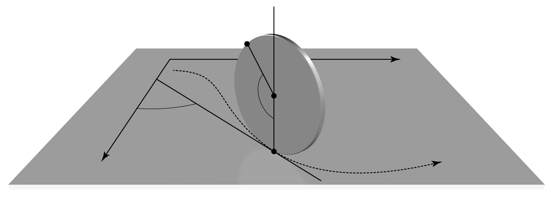
Figure 3.1: Vertical rolling disk.

The constraints of rolling without slipping are

$$\dot{x}=R\cos\varphi\dot{\theta},\qquad\dot{y}=R\sin\varphi\dot{\theta},$$

where $R$ is the radius of the disk, and hence

$$D=\mbox{span}\left\{\partial_{\varphi},\partial_{\theta}+R\cos\varphi\partial_{x}+R\sin\varphi\partial_{y}\right\}.$$ (3.7)

We assume that the disk is homogeneous so the pure kinetic energy Lagrangian is given by

$$L=\frac{1}{2}\left(m(\dot{x}^{2}+\dot{y}^{2})+I\dot{\varphi}^{2}+J\dot{\theta}^{2}\right),$$ (3.8)

where $m$ is the mass of the disk and $I$ and $J$ are the moments of inertia of the disk with respect to the axes that pass through the disk’s center and are, respectively, normal to the plane and normal to the surface of the disk.

The system may be considered as a $G$-Chaplygin system with $G=\mathbb{R}^{2}$ acting by translations. The shape space is the 2-torus $\mathbb{T}^{2}$ with coordinates $(\varphi,\theta)$ and bundle projection $\pi:Q\to\mathbb{T}^{2}$ given by $\pi(x,y,\varphi,\theta)=(\varphi,\theta)$. The horizontal lifts of the coordinate vector fields are

$$\mbox{hor }\partial_{\varphi}=\partial_{\varphi},\qquad\mbox{hor }\partial_{\theta}=\partial_{\theta}+R\cos\varphi\partial_{x}+R\sin\varphi\partial_{y}.$$

Therefore,

$$[\mbox{ hor }\partial_{\varphi},\mbox{ hor }\partial_{\theta}]=-R\sin\varphi\partial_{x}+R\cos\varphi\partial_{y}.$$

It is immediate to check that the above vector field on $Q$ is perpendicular to $D$ given by (3.7) with respect to the Riemannian metric defined by the Lagrangian (3.8). It follows that $\mathcal{P}[\mbox{ hor }\partial_{\varphi},\mbox{ hor }\partial_{\theta}]=0$ and hence also $\mathcal{T}(\partial_{\varphi},\partial_{\theta})=0$. Therefore $\mathcal{T}$ vanishes identically as claimed.

3.2 Almost symplectic structure of the reduced dynamics

The reduced equations for nonholonomic Chaplygin systems can be formulated in almost symplectic form. Namely, the reduced vector field $\overline{X}_{nh}$ describing the reduced dynamics is determined by an equation of the form ${\bf i}_{\overline{X}_{nh}}\Omega_{nh}=dH$, where $H$ is the reduced Hamiltonian and $\Omega_{nh}$ is a non-degenerate 2-form which is not necessarily closed. This structure of the equations seems to have been first noticed by Stanchenko [48, Theorem 1] in the case of an abelian symmetry group $G$, and by Cantrijn et al [12, Equation (17)] in the general case. This formulation of the equations is useful because the gyroscopic reaction forces that make the system non-Hamiltonian are encoded in the ‘non-closed’ part of $\Omega_{nh}$, and this interpretation allows one to give a geometric interpretation of Chaplygin’s multiplier method for Hamiltonisation (see Section 3.5 below).

As explained by Ehlers et al in [14], (see also [28]), a construction of the almost symplectic 2-form $\Omega_{nh}$ may be given utilising the momentum map of the $G$-action and the curvature of the principal connection defined by the constraints. In this section we give an alternative construction of $\Omega_{nh}$ in terms of the gyroscopic 2-form $\Omega_{\mathcal{T}}$, that is defined by (3.13) below using the gyroscopic tensor $\mathcal{T}$ in a way that resembles the definition of the Liouville 1-form on a cotangent bundle. The equivalence of the two approaches is proved at the end of Section 3.6. The main result of this section is Theorem 3.8. We begin with the following:

Proposition 3.6.

The reduced space $\overline{D^{*}}={D^{*}}/G$ is naturally identified with the cotangent bundle $T^{*}S$ (recall that $S=Q/G$ is the shape space).

Proof.

There is a vector bundle isomorphism ${\mathcal{I}}:D/G\to TS$ defined by ${\mathcal{I}}([v])=(T_{q}\pi)(v)$ for $v\in D_{q}$. The inverse morphism is given by ${\mathcal{I}}^{-1}(u)=[\mbox{hor}_{q}u]$, where $u\in T_{\pi(q)}S$, and $\mbox{hor}_{q}:T_{\pi(q)}S\to D_{q}\subseteq T_{q}Q$ is the horizontal lift to $D_{q}$ induced by the principal connection. The dual isomorphisms, ${\mathcal{I}}^{*}:T^{*}S\to\overline{D^{*}}$ and $({\mathcal{I}}^{-1})^{*}:\overline{D^{*}}\to T^{*}S$, define our desired identification and are given by

$${\mathcal{I}}^{*}(\alpha)=[(T_{q}^{*}\pi)(\alpha)_{|D_{q}}],\qquad({\mathcal{I}}^{-1})^{*}([\beta])(u)=\beta(\mbox{hor}_{q}u),$$ (3.9)

for $\alpha\in T^{*}_{\pi(q)}S$, $\beta\in D^{*}_{q}$ and $u\in T_{\pi(q)}S$. ∎

The proposition above allows us to transfer the reduced almost Poisson structure described by Proposition 2.4 on $\overline{D^{*}}$ onto $T^{*}S$. The resulting bracket on $T^{*}S$, that will be denoted by $\{\cdot,\cdot\}_{T^{*}S}$, is again linear and the following proposition, whose proof is postponed until the end of this subsection, gives its description in terms of the gyroscopic tensor $\mathcal{T}$. Note that we continue using the construction outlined in section 2.2 for general vector bundles and identify the linear functions on $T^{*}S$ with vector fields on $S$.

Proposition 3.7.

Let $Y^{\ell},Z^{\ell}$ be the linear functions on $T^{*}S$ corresponding to the vector fields $Y,\,Z\in{\mathfrak{X}}(S)$, and let $f,k$ be basic functions on $T^{*}S$. Then,

$$\begin{split}\{Y^{\ell},Z^{\ell}\}_{T^{*}S}=-[Y,Z]^{\ell}-{\mathcal{T}}(Y,Z)^{\ell},\qquad\{f,Y^{\ell}\}_{T^{*}S}=Y[\tilde{f}]\circ\tau_{S},\qquad\{f,k\}_{T^{*}S}=0,\end{split}$$

where $f=\tilde{f}\circ\tau_{S}$ and $\tau_{S}:T^{*}S\to S$ is the canonical projection.

Let $(s^{1},\dots,s^{r})$ be local coordinates on $S$ and let $(s^{1},\dots,s^{r},p_{1},\dots p_{r})$ be the induced bundle coordinates on $T^{*}S$ (i.e. an element $\alpha\in T^{*}S$ is written as $\alpha=\sum p_{i}ds^{i}$). We have $\left(\frac{\partial}{\partial s^{j}}\right)^{\ell}=p_{j}$ and therefore the above proposition implies that the almost Poisson bracket $\{\cdot,\cdot\}_{T^{*}S}$ is given locally by

$$\{p_{i},p_{j}\}_{T^{*}S}=-\sum_{k=1}^{r}C_{ij}^{k}(s)p_{k},\qquad\{s^{i},p_{j}\}_{T^{*}S}=\delta_{j}^{i},\qquad\{s^{i},s^{j}\}_{T^{*}S}=0,$$ (3.10)

where $\delta_{j}^{i}$ is the Kronecker delta and $C_{ij}^{k}(s)$ are the gyroscopic coefficients determined by (3.6).

Denote by $\Lambda_{T^{*}S}$ the bivector on $T^{*}S$ determined by the almost Poisson bracket $\{\cdot,\cdot\}_{T^{*}S}$, that is,

$$\Lambda_{T^{*}S}(d\varphi,d\mu)=\{\varphi,\mu\}_{T^{*}S},$$

for $\varphi,\mu\in C^{\infty}(T^{*}S)$, and let $\Lambda_{T^{*}S}^{\sharp}$ be vector bundle morphism $\Lambda_{T^{*}S}^{\sharp}:T^{*}(T^{*}S)\to T(T^{*}S)$ defined by $\Lambda_{T^{*}S}^{\sharp}(\beta)=\Lambda_{T^{*}S}(\cdot,\beta)$. Equations (3.10) imply that $\Lambda_{T^{*}S}^{\sharp}$ has block matrix representation

$$\Lambda_{T^{*}S}^{\sharp}=\begin{pmatrix}0&I\\ -I&-\mathcal{C}\end{pmatrix},$$

with respect to the bases $\{ds^{i},dp_{i}\}$ of $T_{(s,p)}^{*}(T^{*}S)$ and $\{\frac{\partial}{\partial s^{j}},\frac{\partial}{\partial p_{j}}\}$ of $T_{(s,p)}(T^{*}S)$. Here $I$ denotes the $r\times r$ identity matrix and $\mathcal{C}$ the $r\times r$ matrix with entries $\mathcal{C}_{ij}=\sum_{k=1}^{r}C_{ij}^{k}(s)p_{k}$. It is clear that the above matrix for $\Lambda_{T^{*}S}^{\sharp}$ is invertible. As a consequence, there is a unique non-degenerate 2-form $\Omega_{nh}$ on $T^{*}S$ whose induced bundle morphism $\Omega_{nh}^{\flat}:T(T^{*}S)\to T^{*}(T^{*}S)$, defined by $\Omega_{nh}^{\flat}:U\mapsto\Omega_{nh}(U,\cdot)={\bf i}_{U}\Omega_{nh}$, is the inverse of $\Lambda_{T^{*}S}^{\sharp}$. Its matrix representation is

$$\Omega_{nh}^{\flat}=(\Lambda_{T^{*}S}^{\sharp})^{-1}=\begin{pmatrix}-\mathcal{C}&-I\\ I&0\end{pmatrix},$$ (3.11)

and so

$$\Omega_{nh}^{\flat}\left(\frac{\partial}{\partial s^{i}}\right)=dp_{i}+\sum_{j,k=1}^{r}C_{ij}^{k}(s)p_{k}\,ds^{j},\qquad\Omega_{nh}^{\flat}\left(\frac{\partial}{\partial p_{i}}\right)=-ds^{i}.$$

Therefore, $\Omega_{nh}$ is locally given by

$$\Omega_{nh}=\sum_{k=1}^{n}ds^{i}\wedge dp_{i}+\sum_{i<j}\sum_{k=1}^{r}C_{ij}^{k}(s)p_{k}\,ds^{i}\wedge ds^{j}.$$ (3.12)

In order to give an intrinsic definition of $\Omega_{nh}$, we start by defining the gyroscopic 2-form $\Omega_{\mathcal{T}}$ on $T^{*}S$ as follows:

$$\Omega_{\mathcal{T}}(\alpha)(U,V):=\alpha\left({\mathcal{T}}((T_{\alpha}\tau_{S})(U),(T_{\alpha}\tau_{S})(V))\right),$$ (3.13)

for $\alpha\in T^{*}S$ and $U,V\in T_{\alpha}(T^{*}S)$, with $\tau_{S}:T^{*}S\to S$ the canonical projection. It is straightforward to check that $\Omega_{\mathcal{T}}$ is semi-basic and that it has the following local expression in bundle coordinates

$$\Omega_{\mathcal{T}}=\sum_{i<j}\sum_{k=1}^{r}C_{ij}^{k}(s)p_{k}\,ds^{i}\wedge ds^{j}.$$ (3.14)

Let $\Omega_{can}$ be the canonical symplectic form on $T^{*}S$. We define $\Omega_{nh}$ intrinsically by:

$$\Omega_{nh}:=\Omega_{can}+\Omega_{\mathcal{T}},$$ (3.15)

so that the local expression (3.12) holds.

We will now formulate the main result of this section. In order to keep the notation simple, we also denote by $H$ and $\overline{X}_{nh}$ the respective pull-backs to $T^{*}S$ of the reduced Hamiltonian $H\in C^{\infty}(\overline{D^{*}})$ and the reduced vector field $\overline{X}_{nh}\in\mathfrak{X}(\overline{D^{*}})$ by the isomorphism ${\mathcal{I}}^{*}:T^{*}S\to\overline{D^{*}}$.

Theorem 3.8.

The 2-form $\Omega_{nh}$ defined by (3.15) is non-degenerate and characterises the reduced vector field $\overline{X}_{nh}$ on $T^{*}S$ uniquely by the relation

$${\bf i}_{\overline{X}_{nh}}\Omega_{nh}=dH,$$ (3.16)

where $H\in C^{\infty}(T^{*}S)$ is the reduced Hamiltonian. Moreover, $\Omega_{nh}$ is closed (and hence symplectic) if and only if the gyroscopic tensor $\mathcal{T}$ vanishes.

Proof.

The non-degeneracy of $\Omega_{nh}$ follows from the local expressions given above. In particular from the matrix representation (3.11) for $\Omega_{nh}^{\flat}$. Now, Proposition 2.5 together with our identification of $\overline{D^{*}}$ with $T^{*}S$ implies that $\Lambda_{T^{*}S}^{\sharp}(dH)=\overline{X}_{nh}$ and therefore $\Omega_{nh}^{\flat}(\overline{X}_{nh})=dH$ which is equivalent to (3.16).

Finally, note that since $\Omega_{can}$ is closed, then $d\Omega_{nh}=d\Omega_{\mathcal{T}}$. Hence, if $\mathcal{T}=0$ then $d\Omega_{nh}=0$. Conversely, suppose that $d\Omega_{nh}=d\Omega_{\mathcal{T}}=0$ and let $\gamma\in\Omega^{1}(S)$. Considering that the vertical lift $\gamma^{\bf v}\in\mathfrak{X}(T^{*}S)$ (defined by (A.4)) is vertical and $\Omega_{\mathcal{T}}$ is semi-basic we have ${\bf i}_{\gamma^{\bf v}}\Omega_{\mathcal{T}}=0$ and therefore

$$0={\bf i}_{\gamma^{\bf v}}d\Omega_{\mathcal{T}}=\mathcal{L}_{\gamma^{\bf v}}\Omega_{\mathcal{T}}=\tau_{S}^{*}(\mathcal{T}_{\gamma}),$$

where $\mathcal{T}_{\gamma}$ is the 2-form on $S$ given by $\mathcal{T}_{\gamma}(s)(u,v)=\langle\gamma(s),\mathcal{T}(u,v)\rangle$ for $s\in S$ and $u,v\in T_{s}S$. Considering that $\tau_{S}^{*}$ is injective, the above equation implies that $\mathcal{T}_{\gamma}=0$ for any 1-form $\gamma$. Hence $\mathcal{T}=0$.

∎

Taking into account (3.16), and the local expression (3.12) of $\Omega_{nh}$, leads to the following local expressions that determine the reduced vector field $\overline{X}_{nh}$:

$$\dot{s}^{i}=\frac{\partial H}{\partial p_{i}},\qquad\dot{p}_{i}=-\frac{\partial H}{\partial s^{i}}-\sum_{j,k=1}^{r}C_{ij}^{k}p_{k}\frac{\partial H}{\partial p_{j}},\qquad i=1,\dots,r.$$ (3.17)

The above equations differ from the standard Hamilton equations by the presence of the terms proportional to the gyroscopic coefficients $C_{ij}^{k}$. These terms correspond to gyroscopic forces that take the system outside of the Hamiltonian realm since, in accordance to the above theorem, $\Omega_{nh}$ is in general not symplectic.

We note that the reduced Hamiltonian $H\in C^{\infty}(T^{*}S)$ is given in bundle coordinates by

$$H(s^{i},p_{i})=\frac{1}{2}\sum_{i,j=1}^{k}K^{ij}(s)p_{i}p_{j}+\overline{U}(s),$$ (3.18)

where $\overline{U}\in C^{\infty}(S)$ is the reduced potential energy induced by the $G$-invariant potential $U\in C^{\infty}(Q)$ and $K^{ij}(s)$ are the entries of the inverse matrix of the positive definite matrix with entries

$$K_{ij}(s)=\left\llangle\mbox{ hor }\frac{\partial}{\partial s^{i}}\,,\,\mbox{ hor }\frac{\partial}{\partial s^{j}}\right\rrangle,$$ (3.19)

where we recall that $\llangle\cdot\,,\,\cdot\rrangle$ is the kinetic energy metric on $Q$. One can easily verify that $K_{ij}$ are well defined functions on the coordinate chart of $S$ by using the $G$-invariance of the kinetic energy and of the horizontal lift. In fact, $(K_{ij})$ is the matrix of the coefficients of the Riemannian metric $\llangle\cdot\,,\,\cdot\rrangle^{-}$ on $S$ characterised by

$$\llangle X,Y\rrangle^{-}\circ\pi_{s}=\llangle\mbox{ hor }X,\mbox{ hor }Y\rrangle,\;\;\mbox{ for }X,Y\in\mathfrak{X}(S).$$ (3.20)

We now use this metric to construct the tensor field ${\mathcal{B}}$ of type $(2,1)$ on $S$ by raising an index of $\mathcal{T}$. Namely, we define

$$\langle{\mathcal{B}}(\alpha,\beta),X\rangle=\langle\alpha,{\mathcal{T}}(\beta^{\sharp},X)\rangle,\;\;\mbox{ for }\alpha,\beta\in\Omega^{1}(S)\mbox{ and }X\in{\mathfrak{X}}(S),$$ (3.21)

where $\beta^{\sharp}\in{\mathfrak{X}}(S)$ denotes the metric dual of the $1$-form $\beta\in\Omega^{1}(S)$ (see (A.2)). Next, we define the semi-basic $1$-form $\eta_{\mathcal{T}}$ on $T^{*}S$ by

$$\eta_{\mathcal{T}}(\alpha)(X)=\langle{\mathcal{B}}(\alpha,\alpha),(T_{\alpha}\tau_{S})(X)\rangle,\;\;\mbox{ for }\alpha\in T^{*}S\mbox{ and }X\in T_{\alpha}(T^{*}S).$$ (3.22)

The 1-form $\eta_{\mathcal{T}}$ encodes the gyroscopic forces that deviate the vector field $\overline{X}_{nh}$ from being Hamiltonian in the manner that is made precise in the following proposition that will be useful ahead.

Proposition 3.9.

We have

$${\bf i}_{\overline{X}_{nh}}\Omega_{can}=dH+\eta_{\mathcal{T}},$$

where $\eta_{\mathcal{T}}$ is the $1$-form on $T^{*}S$ defined by (3.22).

Proof.

In view of the almost symplectic formulation ${\bf i}_{\overline{X}_{nh}}\Omega_{nh}=dH$, and the definition $\Omega_{nh}=\Omega_{can}+\Omega_{\mathcal{T}}$, it suffices to show that $\eta_{\mathcal{T}}=-{\bf i}_{\overline{X}_{nh}}\Omega_{\mathcal{T}}$. Locally we have

$$\mathcal{B}=\sum_{i,j,k,l=1}^{r}C_{ij}^{k}K^{jl}\left(\frac{\partial}{\partial s^{k}}\otimes\frac{\partial}{\partial s^{l}}\right)\otimes ds^{i}.$$

This implies that $\eta_{\mathcal{T}}$ admits the local expression

$$\eta_{\mathcal{T}}=\sum_{i,j,k,l=1}^{r}C_{ij}^{k}K^{jl}p_{k}p_{l}\,ds^{i}.$$ (3.23)

A direct calculation that uses (3.14), (3.17) and (3.18), shows that the right hand side of this equation coincides with the local expression for $-{\bf i}_{\overline{X}_{nh}}\Omega_{\mathcal{T}}$. ∎

We finish this section by presenting the following:

Proof of Proposition 3.7.

The almost-Poisson bracket $\{\cdot,\cdot\}_{T^{*}S}$ on $T^{*}S$ induced by the almost-Poisson bracket $\{\cdot,\cdot\}_{\overline{D^{*}}}$ on $\overline{D^{*}}$ is given by

$$\{\varphi,\mu\}_{T^{*}S}=\{\varphi\circ({\mathcal{I}}^{-1})^{*},\mu\circ({\mathcal{I}}^{-1})^{*}\}_{\overline{D^{*}}}\circ{\mathcal{I}}^{*},$$ (3.24)

for $\varphi,\mu\in C^{\infty}(T^{*}S)$. On the other hand, if $Y\in{\mathfrak{X}}(S)$ and $\tilde{f}\in C^{\infty}(S)$, then (3.9) implies that

$$Y^{\ell}\circ({\mathcal{I}}^{-1})^{*}=(\mbox{ hor }Y)^{\ell},\qquad(\tilde{f}\circ\tau_{S})\circ({\mathcal{I}}^{-1})^{*}=\tilde{f}\circ\overline{\tau},$$ (3.25)

where $\mbox{ hor }X$ is interpreted as a section of $D/G$ in virtue of its equivariance and $\overline{\tau}:\overline{D^{*}}\to S$ denotes the vector bundle projection. Therefore, in view of (3.24), (3.25) and Proposition 2.4, for $\alpha\in T_{\pi(q)}^{*}S$ we have

$$\begin{split}\{Y^{\ell},Z^{\ell}\}_{T^{*}S}(\alpha)&=\{(\mbox{ hor }Y)^{\ell},(\mbox{ hor }Z)^{\ell}\}_{\overline{D^{*}}}({\mathcal{I}}^{*}(\alpha))\\ &=-(\mathcal{P}[\mbox{ hor }Y\,,\,\mbox{ hor }Z])^{\ell}({\mathcal{I}}^{*}(\alpha))\\ &=-\langle{\mathcal{I}}^{*}(\alpha)\,,\,\mathcal{P}[\mbox{ hor }Y\,,\,\mbox{ hor }Z]\rangle\\ &=-\langle T^{*}_{q}\pi(\alpha)\,,\,\mathcal{P}[\mbox{ hor }Y\,,\,\mbox{ hor }Z]\rangle\\ &=-\langle\alpha\,,\,T_{q}\pi\left(\mathcal{P}[\mbox{ hor }Y\,,\,\mbox{ hor }Z]\right)\rangle\\ &=-\langle\alpha\,,\,[Y,Z]+\mathcal{T}(Y,Z)\rangle\\ &=\left(-[Y,Z]^{\ell}-\mathcal{T}(Y,Z)^{\ell}\right)(\alpha),\end{split}$$

where we have used (3.9) to give an expression for ${\mathcal{I}}^{*}(\alpha)$ in the third equality. In a similar manner, but even simpler, we have

$$\begin{split}\{f,Y^{\ell}\}_{T^{*}S}&=\{\tilde{f}\circ\overline{\tau},(\mbox{ hor }Y)^{\ell}\}_{\overline{D^{*}}}\circ{\mathcal{I}}^{*}\\ &=Y[\tilde{f}]\circ\overline{\tau}\circ{\mathcal{I}}^{*}\\ &=Y[\tilde{f}]\circ\tau_{S},\end{split}$$

and

$$\begin{split}\{f,k\}_{T^{*}S}&=\{\tilde{f}\circ\overline{\tau},\tilde{k}\circ\overline{\tau}\}_{\overline{D^{*}}}\circ{\mathcal{I}}^{*}=0.\end{split}$$

∎

3.3 Existence of a smooth invariant measure

One of the most important invariants that a nonholonomic system may have is a smooth volume form. For Chaplygin systems without potential forces, a necessary and sufficient condition for its existence is that a certain 1-form on $S$, that we will denote by $\Theta$, is exact (see Cantrijn et al [12, Theorem 7.5], and also [22, Corollary 4.5]). The 1-form $\Theta$ is naturally constructed as the ordinary contraction of the gyroscopic tensor $\mathcal{T}$:

$$\Theta(Y):=\sum_{j=1}^{r}\langle X^{j}\,,\,\mathcal{T}(X_{j},Y)\rangle,$$ (3.26)

where $\{X_{1},\dots X_{r}\}$ is a local basis of vector fields of $S$, $\{X^{1},\dots X^{r}\}$ is the dual basis, and $\langle\cdot\,,\,\cdot\rangle$ denotes the pairing of covectors and vectors on $S$. It is clear that $\Theta$ is well-defined (globally and independently of the basis). A local expression for $\Theta$ may be obtained by taking $\{\frac{\partial}{\partial s^{j}}\}$ as the basis of vector fields $\{X_{j}\}$ in its definition. In view of the definition of the gyroscopic coefficients, we get $\Theta\left(\frac{\partial}{\partial s^{i}}\right)=\sum_{j=1}^{r}C_{ji}^{j}(s)$, and, therefore, $\Theta$ is locally given by

$$\Theta=\sum_{i,j=1}^{r}C_{ji}^{j}(s)\,ds^{i}.$$ (3.27)

Recall that the cotangent bundle $T^{*}S$ is equipped with the Liouville volume form $\nu$ defined as $\nu:=\Omega_{can}^{r}$.

Definition 3.10.

A volume form $\mu$ on $T^{*}S$ is basic if its density with respect to the Liouville volume form $\nu$ is a basic function. Namely if

$$\mu=(f\circ\tau_{S})\,\nu,$$

for a positive function $f\in C^{\infty}(S)$.

The relationship between $\Theta$ and the existence of an invariant measure is given in the following theorem.

Theorem 3.11 (Cantrijn et al. [12]).

Let $\nu=\Omega_{can}^{r}$ be the Liouville volume form on $T^{*}S$.

1. For a Hamiltonian $H=K+U$, the reduced equations of motion of a nonholonomic Chaplygin system preserve the basic measure

   $$\mu=\exp(\sigma\circ\tau_{S})\,\nu,\qquad\sigma\in C^{\infty}(S),$$ (3.28)

   if and only if $\Theta$ is exact with $\Theta=d\sigma$.

2. In the absence of potential energy, the reduced equations posses a smooth invariant measure if and only if it is basic (which is then characterised by item (i)).

Remark 3.12.

In section 4.1 below we give an example of a Chaplygin system with non-trivial potential possessing a smooth invariant measure that is not basic. Such example shows that the conclusion of item (ii) may not be extended to systems with potential energy.

Theorem 3.11 was proved in [12] (see also [22]) with an alternative definition of the 1-form $\Theta$. Here we present an alternative intrinsic proof which is based on the following lemma. In its statement, recall that $\Theta^{\sharp}\in\mathfrak{X}(S)$ denotes the metric dual of $\Theta\in\Omega^{1}(S)$ (see (A.2)), and $(\Theta^{\sharp})^{\ell}\in C^{\infty}(T^{*}S)$ is the associated linear function (see (A.1)).

Lemma 3.13.

Let $\mu$ be a general (not necessarily basic) volume form on $T^{*}S$ given by $\mu=\exp{(\overline{\sigma})}\nu$, with $\overline{\sigma}\in C^{\infty}(T^{*}S)$ and where as usual $\nu$ is the Liouville measure on $T^{*}S$. Denote by ${\mathcal{L}}_{\overline{X}_{nh}}$ the Lie derivative operator with respect to $\overline{X}_{nh}$. Then

$${\mathcal{L}}_{\overline{X}_{nh}}(\mu)=(\overline{X}_{nh}[\overline{\sigma}]-(\Theta^{\sharp})^{\ell})\,\mu.$$ (3.29)

The proof of this lemma is postponed to the end of the section and we proceed to give the proof of Theorem 3.11.

Proof of Theorem 3.11.

To prove item $(i)$ consider the basic measure $\mu=\exp(\sigma\circ\tau_{S})\nu$ with $\sigma\in C^{\infty}(S)$. Using the local expressions (3.17) and (3.18) for $\overline{X}_{nh}$ one shows that $\overline{X}_{nh}[\sigma\circ\tau_{S}]=(d\sigma^{\sharp})^{\ell}$. Hence, in this case, (3.29) may be written as

$${\mathcal{L}}_{\overline{X}_{nh}}(\mu)=((d\sigma^{\sharp})^{\ell}-(\Theta^{\sharp})^{\ell})\,\mu,$$

which implies that ${\mathcal{L}}_{\overline{X}_{nh}}(\mu)=0$ if and only if $(d\sigma^{\sharp})^{\ell}-(\Theta^{\sharp})^{\ell}=0$ or, equivalently, $d\sigma=\Theta$.

Next, we will prove item $(ii)$ of the theorem. Suppose that the volume form $\mu=\exp(\overline{\sigma})\nu$ is invariant under the action of $\overline{X}_{nh}$. Then (3.29) implies that $\overline{X}_{nh}[\overline{\sigma}]=(\Theta^{\sharp})^{\ell}$ and therefore, for any $\gamma\in\Omega^{1}(S)$, we have

$$(\gamma^{\bf v}[\overline{X}_{nh}[\overline{\sigma}]])\circ 0=(\gamma^{\bf v}[(\Theta^{\sharp})^{\ell}])\circ 0=\langle\gamma,\Theta^{\sharp}\rangle\circ\tau_{S},$$ (3.30)

where $0:S\to T^{*}S$ is the zero section of the vector bundle $\tau_{S}:T^{*}S\to S$.

On the other hand, using the local equations (3.17) and (3.18) which determine to the vector field $\overline{X}_{nh}$ and the local expression (A.6) of the vector field $\gamma^{\bf v}$, we conclude that

$$(\gamma^{\bf v}[\overline{X}_{nh}[\overline{\sigma}]])\circ 0=\langle\gamma,(d\sigma)^{\sharp}\rangle\circ\tau_{S},\;\;\;\forall\gamma\in\Omega^{1}(S)$$

with $\sigma=\overline{\sigma}\circ 0\in C^{\infty}(S)$. So, from (3.30), we deduce that

$$\langle\gamma,(d\sigma)^{\sharp}\rangle\circ\tau_{S}=\langle\gamma,\Theta^{\sharp}\rangle\circ\tau_{S},\;\;\forall\gamma\in\Omega^{1}(S)$$

which implies that $d\sigma=\Theta$. Thus, using item $(i)$, it follows that the basic volume form $\exp({\sigma}\circ\tau_{S})\nu$ is invariant under the action of $\overline{X}_{nh}$. ∎

We now present the following:

Corollary 3.14 (Stanchenko [48]).

The existence of a basic invariant measure for a $G$-Chaplygin nonholonomic system is weakly Noetherian. Namely, if a $G$-Chaplygin nonholonomic system preserves a basic measure, then it continues to preserve the same basic measure under the addition of a $G$-invariant potential.

Proof.

The gyroscopic tensor $\mathcal{T}$ only depends on the kinetic energy and not on the potential. Thus, the same is true for the 1-form $\Theta$. In virtue of item (i) of Theorem 3.11, the preservation of a basic measure is equivalent to the exactness of $\Theta$, which holds independently of the potential. ∎

We finish the section with the proof of Lemma 3.13.

Proof.

Using the basic properties of the Lie derivative we have

$${\mathcal{L}}_{\overline{X}_{nh}}(\mu)={\mathcal{L}}_{\overline{X}_{nh}}(\exp(\overline{\sigma})\nu)=\exp(\overline{\sigma})(\overline{X}_{nh}[\overline{\sigma}]\nu+r\,({\mathcal{L}}_{\overline{X}_{nh}}\Omega_{can})\wedge\Omega_{can}^{r-1}).$$ (3.31)

On the other hand, using Cartan’s magic formula and the fact that $\Omega_{can}$ is closed, we get

$${\mathcal{L}}_{\overline{X}_{nh}}\Omega_{can}={\bf i}_{\overline{X}_{nh}}(d\Omega_{can})+d({\bf i}_{\overline{X}_{nh}}\Omega_{can})=d({\bf i}_{\overline{X}_{nh}}\Omega_{can}),$$

which, in view of Proposition 3.9 allows us to write (3.31) as

$${\mathcal{L}}_{\overline{X}_{nh}}(\mu)=\exp(\overline{\sigma})(\overline{X}_{nh}[\overline{\sigma}]\nu+r\,d\eta_{\mathcal{T}}\wedge\Omega_{can}^{r-1}).$$ (3.32)

However we claim that

$$r\,d\eta_{\mathcal{T}}\wedge\Omega_{can}^{r-1}=-(\Theta^{\sharp})^{\ell}\,\nu.$$ (3.33)

Note that substitution of (3.33) into (3.32) proves the lemma, so it only remains to prove that (3.33) holds.

Let $\{X_{i}\}$ be a local basis of $\mathfrak{X}(S)$ and $\{X^{i}\}$ be the dual basis of $\Omega^{1}(S)$. To prove (3.33) we will show that the following two identities hold:

$$(\Theta^{\sharp})^{\ell}=-\sum_{i=1}^{r}d\eta_{\mathcal{T}}\left(X_{i}^{*c},(X^{i})^{\bf v}\right),\qquad\qquad rd\eta_{\mathcal{T}}\wedge\Omega_{can}^{r-1}=\sum_{i=1}^{r}d\eta_{\mathcal{T}}(X_{i}^{*c},(X^{i})^{\bf v})\nu,$$ (3.34)

where the vertical lifts $(X^{i})^{\bf v}$ and the complete lifts $X_{i}^{*c}$ are respectively defined in (A.4) and (A.5).

Starting from the local expression (3.23) of $\eta_{\mathcal{T}}$ and using (A.6), we have

$$\eta_{\mathcal{T}}(\alpha^{\bf v})=0,\qquad\eta_{\mathcal{T}}(Y^{*c})=\sum_{i,j,k,l=1}^{r}Y^{i}C_{ij}^{k}K^{jl}p_{k}p_{l},$$ (3.35)

for $\alpha\in\Omega^{1}(S)$ and $Y\in\mathfrak{X}(S)$. So, if $({\mathcal{B}},Y)$ is the tensor of type $(2,0)$ on $S$ given by

$$({\mathcal{B}},Y)(\alpha,\beta)=\langle\mathcal{B}(\alpha,\beta),Y\rangle=\langle\alpha,{\mathcal{T}}(\beta^{\sharp},Y)\rangle,\mbox{ for }\alpha,\beta\in\Omega^{1}(S),$$ (3.36)

it follows that the quadratic function $({\mathcal{B}},Y)^{\mathfrak{q}}$ on $T^{*}S$ (see (A.9)) is just $-\eta_{\mathcal{T}}(Y^{*c})$. Thus, using (A.8) and (3.35), we deduce that

$$d\eta_{\mathcal{T}}(\alpha^{\bf v},Y^{*c})=\alpha^{\bf v}(\eta_{\mathcal{T}}(Y^{*c}))-Y^{*c}(\eta_{\mathcal{T}}(\alpha^{\bf v}))-\eta_{\mathcal{T}}[\alpha^{\bf v},Y^{*c}]=-\alpha^{\bf v}(({\mathcal{B}},Y)^{\mathfrak{q}}).$$

This implies that

$$d\eta_{\mathcal{T}}(\alpha^{\bf v},Y^{*c})=\sum_{i,j,k,l=1}^{r}Y^{i}\alpha_{l}(C_{ij}^{k}K^{jl}+C_{ij}^{l}K^{jk})p_{k}$$

or, equivalently,

$$d\eta_{\mathcal{T}}(\alpha^{\bf v},Y^{*c})=-({\mathcal{T}}(\alpha^{\sharp},Y))^{\ell}-(({\mathcal{B}},Y)(\alpha,\cdot))^{\ell},$$

where $({\mathcal{B}},Y)(\alpha,\cdot)$ is the vector field on $S$ which is characterized by

$$\langle\beta,({\mathcal{B}},Y)(\alpha,\cdot)\rangle=({\mathcal{B}},Y)(\alpha,\beta),\;\;\mbox{ for }\beta\in\Omega^{1}(S).$$

Therefore,

$$\sum_{i=1}^{r}d\eta_{\mathcal{T}}\left(X_{i}^{*c},(X^{i})^{\bf v}\right)=\sum_{i=1}^{r}({\mathcal{T}}((X^{i})^{\sharp},X_{i}))^{\ell}+\sum_{i=1}^{r}(({\mathcal{B}},X_{i})(X^{i},\cdot))^{\ell}.$$

Now, since the gyroscopic tensor $\mathcal{T}$ is skew-symmetric, ${\mathcal{T}}((X^{i})^{\sharp},X_{i})=0$, for all $i$. In fact, if our local basis $\{X_{i}\}$ is orthonormal then $(X^{i})^{\sharp}=X_{i}$, for all $i$. Consequently,

$$\sum_{i=1}^{r}d\eta_{\mathcal{T}}\left(X_{i}^{*c},(X^{i})^{\bf v}\right)=\sum_{i=1}^{r}(({\mathcal{B}},X_{i})(X^{i},\cdot))^{\ell}.$$ (3.37)

On the other hand, in view of the local expression (3.27) of $\Theta$ and using (3.36), we have

$$\Theta(\alpha^{\sharp})=-\langle\alpha,\sum_{i=1}^{r}({\mathcal{B}},X_{i})(X^{i},\cdot)\rangle,\;\;\mbox{ for }\alpha\in\Omega^{1}(S).$$

This implies that

$$\Theta^{\sharp}=-\sum_{i=1}^{r}({\mathcal{B}},X_{i})(X^{i},\cdot)$$

and, by (3.37), it follows that

$$(\Theta^{\sharp})^{\ell}=-\sum_{i=1}^{r}d\eta_{\mathcal{T}}\left(X_{i}^{*c},(X^{i})^{\bf v}\right),$$

which proves that the first identity in (3.34) holds.

Now, (A.6) shows that $\{X_{i}^{*c},(X^{i})^{\bf v}\}$ is a local basis of $\mathfrak{X}(T^{*}S)$ and, moreover,

$$\Omega_{can}(Y^{*c},\alpha^{\bf{v}})=\alpha(Y)\circ\tau_{S},\;\;\mbox{ for }Y\in\mathfrak{X}(S)\mbox{ and }\alpha\in\Omega^{1}(S).$$ (3.38)

Thus, we deduce that

$$\begin{split}(r\,d\eta_{\mathcal{T}}\wedge\Omega_{can}^{r-1})&(X_{1}^{*c},(X^{1})^{\bf v},\dots,X_{r}^{*c},(X^{r})^{\bf v})=\\ &=r\sum_{i=1}^{r}d\eta_{\mathcal{T}}(X_{i}^{*c},(X^{i})^{\bf v})\Omega_{can}^{r-1}(X_{1}^{*c},(X^{1})^{\bf v},\dots,\widehat{X_{i}^{*c}},\widehat{(X^{i})^{\bf v}},\dots,X_{r}^{*c},(X^{r})^{\bf v})\\ &=r!\sum_{i=1}^{r}d\eta_{\mathcal{T}}(X_{i}^{*c},(X^{i})^{\bf v}).\end{split}$$

On the other hand, using (3.38), it also follows that

$$\nu(X_{1}^{*c},(X^{1})^{\bf v},\dots,X_{r}^{*c},(X^{r})^{\bf v})=r!$$

which shows that the second equation in (3.34) also holds. ∎

3.4 Chaplygin Hamiltonisation

Within the class of Chaplygin systems with an invariant measure there is a special subclass whose equations of motion may be written in Hamiltonian form after a time reparametrisation $dt=g(s)\,d\tau$, for a positive function $g\in C^{\infty}(S)$. This observation goes back to Chaplygin who introduced his reducing multiplier method [13]. The geometric formulation of this procedure was given first by Stanchenko [48]. Given that the time reparametrisation corresponds to the vector field rescaling $\overline{X}_{nh}\mapsto g\overline{X}_{nh}$, we define:

Definition 3.15.

A nonholonomic Chaplygin system is said to be Hamiltonisable if there exists a positive function $g\in C^{\infty}(S)$ and a symplectic form $\overline{\Omega}$ on $T^{*}S$ such that the rescaled vector field $g\overline{X}_{nh}$ satisfies

$${\bf i}_{g\overline{X}_{nh}}\overline{\Omega}=dH.$$

In this case we say that the vector field $\overline{X}_{nh}$ is conformally Hamiltonian and that the system is Hamiltonisable with the time reparametrisation $dt=g(s)\,d\tau$.

In this paper it will always be the case that the 2-form $\overline{\Omega}=g^{-1}\Omega_{nh}$. So the task is to determine conditions that guarantee that $\Omega_{nh}$ is closed after multiplication by a positive function $g^{-1}$. If such a function exists we shall say that $\Omega_{nh}$ is conformally symplectic and the function $g^{-1}$ will be called the conformal factor. A characterisation of the condition that $\Omega_{nh}$ is conformally symplectic is given in our main Theorem 3.21 ahead in terms of the gyroscopic tensor.

Remark 3.16.

We note that according to [48, 14], one could more generally have $\overline{\Omega}=g^{-1}(\Omega_{nh}+\Omega_{0})$ where the degenerate 2-form $\Omega_{0}$ satisfies ${\bf i}_{\overline{X}_{nh}}\Omega_{0}=0$. The possibility of achieving a Hamiltonisation with $\Omega_{0}\neq 0$, is not considered in this paper and therefore our approach only leads to sufficient conditions for Hamiltonisation.

Remark 3.17.

In many references Chaplygin’s Hamiltonisation procedure is presented as a time reparametrisation together with a rescaling of the momenta. From the geometric perspective, the rescaling of the momenta serves to obtain Darboux coordinates for the symplectic form $\overline{\Omega}$. This is illustrated in our treatment of the nonholonomic particle in Section 4.1.

Below we show that a Hamiltonisable Chaplygin system indeed admits an invariant measure. This is a well-known result appearing in various references, e.g. [20, 14], and which is a consequence of the following general observation for conformally Hamiltonian systems.

Proposition 3.18.

Let $\overline{\Omega}$ a symplectic structure on a manifold $P$ of dimension $2r$, $\overline{X}$ a vector field on $P$ and $g$ a real positive $C^{\infty}$-function on $P$ such that $g\overline{X}$ is Hamiltonian vector field with respect to the symplectic structure $\overline{\Omega}$. Then, $g\overline{\Omega}^{r}$ is an invariant measure for $\overline{X}$.

Proof.

Since $g\overline{X}$ is a Hamiltonian vector field with respect to the symplectic structure $\overline{\Omega}$, it follows that $\overline{\Omega}^{r}$ is an invariant measure for $g\overline{X}$. Thus, using the properties of the Lie derivative operator ${\mathcal{L}}$, we have that

$$0={\mathcal{L}}_{g\overline{X}}\overline{\Omega}^{r}=g{\mathcal{L}}_{\overline{X}}\overline{\Omega}^{r}+dg\wedge i_{\overline{X}}\overline{\Omega}^{r}.$$

On the other hand, considering that $dg\wedge\overline{\Omega}^{r}$ is a $(2r+1)$-form on $P$, it identically vanishes, and hence

$$0=i_{\overline{X}}(dg\wedge\overline{\Omega}^{r})=\overline{X}[g]\overline{\Omega}^{r}-dg\wedge i_{\overline{X}}\overline{\Omega}^{r}.$$

Therefore, using the properties of the Lie derivative and the above equalities, we have

$${\mathcal{L}}_{\overline{X}}(g\overline{\Omega}^{r})=g\,{\mathcal{L}}_{\overline{X}}\overline{\Omega}^{r}+\overline{X}[g]\overline{\Omega}^{r}=0.$$

∎

3.5 $\phi$-simple Chaplygin systems and Hamiltonisation

We now introduce the notion of a $\phi$-simple Chaplygin system that is central to the results of our paper.

Definition 3.19.

A non-holonomic Chaplygin system is said to be $\phi$-simple, if there exists a function $\phi\in C^{\infty}(S)$ such that the gyroscopic tensor ${\mathcal{T}}$ satisfies

$${\mathcal{T}}(Y,Z)=Z[\phi]Y-Y[\phi]Z,$$ (3.39)

for all $Y,Z\in{\mathfrak{X}}(S)$.

Remark 3.20.

Considering that the definition of the gyroscopic tensor $\mathcal{T}$ is independent of the potential energy, we conclude that the notion of $\phi$-simplicity is weakly Noetherian. Namely, if a $G$-Chaplygin nonholonomic system is $\phi$-simple, then it continues to be $\phi$-simple under the addition of a $G$-invariant potential.

The following is the main result of the paper:

Theorem 3.21.

1. A nonholonomic Chaplygin system is $\phi$-simple if and only if $\Omega_{nh}$ is conformally symplectic with conformal factor $\exp(\phi\circ\tau_{S})$ (i.e. $d(\exp(\phi\circ\tau_{S})\Omega_{nh}=0$).

2. The reduced equations of motion of a $\phi$-simple non-holonomic Chaplygin system possess the basic invariant measure $\mu=\exp(\sigma\circ\tau_{S})\,\nu$, where $\nu$ is the Liouville measure and $\sigma=(r-1)\phi$.

3. If $r=2$ then statement (ii) may be inverted: if the reduced equations of motion possess the basic invariant measure $\mu=\exp(\phi\circ\tau_{S})\,\nu$, then the system is $\phi$-simple.

In particular, item $(i)$ implies:

Corollary 3.22.

A $\phi$-simple Chaplygin system is Hamiltonisable after the time reparametrisation $dt=\exp(-\phi(s))\,d\tau$.

Remark 3.23.

Recently Jovanović [35] proved the existence of a Chaplygin system with $r>2$ degrees of freedom that possesses an invariant measure but does not allow a Hamiltonisation, and hence is not $\phi$-simple. This shows that the reciprocal of the statement in item $(ii)$ is not true in general if $r>2$. Another example of this instance is the Chaplygin sphere treated as a Chaplygin system with $G=\mathbb{R}^{2}$. The system has an invariant measure but, as shown in [14, Section 3], the system does not allow a Hamiltonisation at the $T^{*}\mathrm{SO}(3)$ level.

For the proof of Theorem 3.21 we will require the following.

Lemma 3.24.

The following conditions are equivalent:

1. $\Omega_{nh}$ is conformally symplectic with conformal factor $\exp(\phi\circ\tau_{S})$,

2. $d\Omega_{nh}=-d(\phi\circ\tau_{S})\wedge\Omega_{nh}$,

3. The gyroscopic 2-form $\Omega_{\mathcal{T}}=\lambda_{S}\wedge d(\phi\circ\tau_{S})$, where $\lambda_{S}$ is the Liouville $1$-form on $T^{*}S$ given by

   $$\lambda_{S}(\alpha)(U)=\alpha((T_{\alpha}\tau_{S})(U)),\;\;\mbox{ for }\alpha\in T^{*}S\mbox{ and }U\in T_{\alpha}(T^{*}S).$$ (3.40)

Proof.

We have

$$d(\exp(\phi\circ\tau_{S})\Omega_{nh})=\exp(\phi\circ\tau_{S})\ \left(d(\phi\circ\tau_{S})\wedge\Omega_{nh}+d\Omega_{nh}\right)$$

which shows the equivalence of $(i)$ and $(ii)$.

$(iii)$ $\implies$ $(i)$ This result was first proved by Stanchenko [48, Proposition 2] (see also Cantrijn et al [12, Equation (18)]). For the sake of completeness, we present a proof here. Using that $\Omega_{nh}=\Omega_{can}+\Omega_{\mathcal{T}}$ and that $d\Omega_{can}=0$, we have

$$\begin{split}d\left(\exp(\phi\circ\tau_{S})\Omega_{nh}\right)&=\exp\left(\phi\circ\tau_{S}\right)\left(d(\phi\circ\tau_{s})\wedge(\Omega_{can}+\Omega_{\mathcal{T}})+d\Omega_{\mathcal{T}}\right)\\ &=\exp\left(\phi\circ\tau_{S}\right)\left(d(\phi\circ\tau_{s})\wedge\Omega_{can}+d\Omega_{\mathcal{T}}\right),\end{split}$$

where we have used $d(\phi\circ\tau_{s})\wedge\Omega_{\mathcal{T}}=0$ in the second equality as is implied by item $(iii)$. On the other hand, taking the exterior differential in the expression $\Omega_{\mathcal{T}}=\lambda_{S}\wedge d(\phi\circ\tau_{S})$ and using the well-known relation $d\lambda_{S}=-\Omega_{can}$ yields

$$d\Omega_{\mathcal{T}}=-d(\phi\circ\tau_{S})\wedge\Omega_{can},$$

which shows that $d(\exp(\phi\circ\tau_{S})\Omega_{nh})=0$.

$(ii)$ $\implies$ $(iii)$ Starting from $d\Omega_{nh}=-d(\phi\circ\tau_{S})\wedge\Omega_{nh}$ and using that $\Omega_{nh}=\Omega_{can}+\Omega_{\mathcal{T}}$ and $d\Omega_{can}=0$, we deduce that

$$d\Omega_{\mathcal{T}}=-d(\phi\circ\tau_{S})\wedge\Omega_{can}-d(\phi\circ\tau_{S})\wedge\Omega_{\mathcal{T}}.$$ (3.41)

Now, let $\gamma\in\Omega^{1}(S)$ and $\gamma^{\bf v}\in\mathfrak{X}(T^{*}S)$ be its vertical lift (see (A.4)). Then, since $\gamma^{\bf v}$ is a vertical vector field (see e.g. (A.6)) and the 2-form $\Omega_{\mathcal{T}}$ is semi-basic, we obtain the identities

$${\bf i}_{\gamma^{\bf v}}(d(\phi\circ\tau_{S}))=0,\qquad i_{\gamma^{\bf v}}\Omega_{\mathcal{T}}=0.$$

Therefore, from (3.41), we have that

$${\bf i}_{\gamma^{\bf v}}d\Omega_{\mathcal{T}}=d(\phi\circ\tau_{S})\wedge i_{\gamma^{\bf v}}\Omega_{can},$$ (3.42)

which in view of (A.7) becomes

$${\bf i}_{\gamma^{\bf v}}d\Omega_{\mathcal{T}}=-d(\phi\circ\tau_{S})\wedge\tau_{S}^{*}\gamma.$$

In particular, we obtain that

$$({\bf i}_{\gamma^{\bf v}}d\Omega_{\mathcal{T}})\circ\gamma=-(d(\phi\circ\tau_{S})\wedge\tau_{S}^{*}\gamma)\circ\gamma.$$ (3.43)

In addition, using the local expressions of the $2$-form $\Omega_{\mathcal{T}}$, given respectively by (3.14) and (A.6), we can prove that

$$({\bf i}_{\gamma^{\bf v}}d\Omega_{\mathcal{T}})\circ\gamma=\Omega_{\mathcal{T}}\circ\gamma.$$ (3.44)

Moreover, the definition (3.40) of the Liouville $1$-form $\lambda_{S}$, implies that

$$\left(\lambda_{S}(\gamma(s))\right)(U)=\gamma(s)\left((T_{\gamma(s)}\tau_{S})(U)\right)=\left(\tau_{S}^{*}\gamma\right)(\gamma(s))(U),$$

for $s\in S$ and $U\in T_{\gamma(s)}(T^{*}S)$. In other words,

$$\lambda_{S}\circ\gamma=(\tau_{S}^{*}\gamma)\circ\gamma.$$

Thus, from (3.43) and (3.44), we conclude that

$$\Omega_{\mathcal{T}}\circ\gamma=-(d(\phi\circ\tau_{S})\wedge\lambda_{S})\circ\gamma,$$

and since the $1$-form $\gamma$ is arbitrary we obtain

$$\Omega_{\mathcal{T}}=\lambda_{S}\wedge d(\phi\circ\tau_{S}),$$

as required. ∎

We are now ready to present the proof of Theorem 3.21.

Proof.

(of Theorem 3.21) $(i)$ Suppose that the system is $\phi$-simple so (3.39) holds. Using this equation in the definition (3.13) of $\Omega_{\mathcal{T}}$ we have that, for $\alpha\in T^{*}S$ and $U,V\in T_{\alpha}(T^{*}S)$

$$\begin{split}\Omega_{\mathcal{T}}(\alpha)(U,V)&=d\phi(T_{\alpha}\tau_{S}V)\alpha(T_{\alpha}\tau_{S}(U))-d\phi(T_{\alpha}\tau_{S}U)\alpha(T_{\alpha}\tau_{S}(V))\\ &=d(\phi\circ\tau_{S})(\alpha)(V)\lambda_{S}(\alpha)(U)-d(\phi\circ\tau_{S})(\alpha)(U)\lambda_{S}(\alpha)(V)\\ &=\lambda_{S}\wedge d(\phi\circ\tau_{S})(\alpha)(U,V).\end{split}$$

So, it follows that $\Omega_{\mathcal{T}}=\lambda_{S}\wedge d(\phi\circ\tau_{S})$ and Lemma 3.24 implies that $d(\exp(\phi\circ\tau_{S})\Omega_{nh})=0$ as required.

Conversely, assume that $d(\exp(\phi\circ\tau_{S})\Omega_{nh})=0$. Then, using again Lemma 3.24, we deduce that $\Omega_{\mathcal{T}}=\lambda_{S}\wedge d(\phi\circ\tau_{S})$. So, from the definition (3.13) of $\Omega_{\mathcal{T}}$ we obtain

$$\begin{split}&\alpha\left({\mathcal{T}}(\tau_{S}(\alpha))((T_{\alpha}\tau_{S})(U),(T_{\alpha}\tau_{S})(V)\right)=\\ &\qquad\qquad\qquad\alpha\left((T_{\alpha}\tau_{S})(V)[\phi](T_{\alpha}\tau_{S})(U)-(T_{\alpha}\tau_{S})(U)[\phi](T_{\alpha}\tau_{S})(V)\right).\end{split}$$

Therefore, since $\tau_{S}$ is a submersion, we conclude that

$${\mathcal{T}}(s)(Y,Z)=Z[\phi]Y-Y[\phi]Z,\;\;\mbox{ for }Y,Z\in T_{s}S,$$

that is, the system is $\phi$-simple.

$(ii)$ This is a consequence of item $(i)$ and Proposition 3.18 but we present a simple alternative proof. Suppose that the system is $\phi$-simple so (3.39) holds and let $\sigma=(r-1)\phi$. Let $Y\in\mathfrak{X}(S)$, then the 1-form $\Theta$ defined by (3.26) satisfies

$$\begin{split}\Theta(Y)&=\sum_{i=1}^{r}\left\langle X^{i}\,,\,\left(Y[\phi]X_{i}-X_{i}[\phi]Y\right)\right\rangle\\ &=rY[\phi]-\sum_{i=1}^{k}\langle X_{i},Y\rangle X_{i}[\phi]\\ &=(r-1)Y[\phi].\end{split}$$

Therefore $\Theta=d\sigma$ and Theorem 3.11 implies the preservation of the measure $\mu=\exp(\sigma)\,\nu$.

$(iii)$ Now suppose that $r=2$ and that the reduced equations of motion preserve the basic measure $\mu=\exp(\phi\circ\tau_{S})\,\nu$. Then item $(i)$ of Theorem 3.11 implies that $\Theta=d\phi$. In view of the local expression (3.27) for $\Theta$ we obtain the following relations between the partial derivatives of $\phi$ and the gyroscopic coefficients:

$$\frac{\partial\phi}{\partial s^{1}}=C_{21}^{2}(s),\qquad\frac{\partial\phi}{\partial s^{2}}=C_{12}^{1}(s).$$

Therefore,

$$\begin{split}{\mathcal{T}}\left(\frac{\partial}{\partial s^{1}},\frac{\partial}{\partial s^{2}}\right)&=C_{12}^{1}(s)\frac{\partial}{\partial s^{1}}+C_{12}^{2}(s)\frac{\partial}{\partial s^{2}}\\ &=\frac{\partial\phi}{\partial s^{2}}\frac{\partial}{\partial s^{1}}-\frac{\partial\phi}{\partial s^{1}}\frac{\partial}{\partial s^{2}}.\end{split}$$

The above expression shows that the $\phi$-simplicity relation (3.39) holds for the basis $\{\frac{\partial}{\partial s^{1}},\frac{\partial}{\partial s^{2}}\}$, and hence, by linearity, for general $Y,Z\in\mathfrak{X}(S)$. ∎

Corollary 3.25.

1. A purely kinetic, nonholonomic Chaplygin system with 2 degrees of freedom possesses an invariant measure if and only if it is $\phi$-simple.

2. [Chaplygin’s Reducing Multiplier Theorem [13]] If a Chaplygin system with 2 degrees of freedom preserves the basic measure $\mu=\exp(\sigma\circ\tau_{S})\,\nu$, then the system is Hamiltonisable after the time reparametrisation $dt=\exp(-\sigma(s))\,d\tau$.

3. The Hamiltonisation of a $\phi$-simple Chaplygin system by the time reparametrisation
   $dt=\exp(-\sigma(s))\,d\tau$ is weakly Noetherian. Namely, the same time reparametrisation Hamiltonises the system under the addition of an arbitrary $G$-invariant potential.

Proof.

$(i)$ is a direct consequence of item $(ii)$ of Theorem 3.11 and item $(iii)$ of Theorem 3.21. Item $(ii)$ follows from item $(i)$ and Corollary 3.22. Finally, item $(iii)$ follows from Remark 3.20. ∎

We now show that the sufficient conditions for Hamiltonisation that were recently obtained in García-Naranjo [25] are equivalent to $\phi$-simplicity. For this matter we recall the so-called hypothesis (H) from this reference:

(H).

The gyroscopic coefficients $C_{ij}^{k}$ written in the coordinates $(s^{1},\dots,s^{r})$ satisfy:

$$C_{ij}^{k}=0,\quad\mbox{for}\quad k\neq i\neq j\neq k,\qquad C_{ij}^{j}=C_{ik}^{k}\quad\mbox{for all }\quad j,k\neq i.$$

It is shown in [25] that (H) is an intrinsic condition (independent of the choice of coordinates). Moreover, in this reference it is also shown that if (H) holds, and the basic measure $\mu=\exp(\sigma)\nu$ is preserved by the reduced flow, then the system is Hamiltonisable with the time reparametrisation $dt=\exp(\sigma/(1-r))\,d\tau$. Proposition 3.26 below shows that these two hypothesis taken together are equivalent to the condition that the system is $\phi$-simple with $\phi=\sigma/(r-1)$, so the Hamiltonisation result of [25] is a particular consequence of Corollary 3.22.

Before presenting Proposition 3.26 and its proof, we note that (H) is equivalent to the existence of a 1-form $\beta$ on $S$ such that the gyroscopic tensor satisfies ${\mathcal{T}}(Y,Z)=\beta(Z)Y-\beta(Y)Z$, for vector fields $Y,Z\in\mathfrak{X}(S)$. In this case, using its definition (3.26), it is easy to show that the 1-form $\Theta=(r-1)\beta$. Therefore, the condition (H) may be reformulated as:

(H’).

The gyroscopic tensor satisfies

$${\mathcal{T}}(Y,Z)=\frac{1}{r-1}\left(\Theta(Z)Y-\Theta(Y)Z\right),$$

for vector fields $Y,Z\in\mathfrak{X}(S)$.

Proposition 3.26.

A Chaplygin system is $\phi$-simple if and only if (H) holds and the reduced equations of motion preserve the invariant measure $\mu=\exp(\sigma)\nu$ with $\sigma=(r-1)\phi$ (where, as usual, $\nu$ is the Liouville measure in $T^{*}S$).

Proof.

Suppose that the Chaplygin system under consideration is $\phi$-simple. Then, item $(ii)$ of Theorem 3.21 implies that the measure $\mu=\exp(\sigma)\nu$ in the statement of the proposition is preserved by the flow of the reduced system. Moreover, because of item $(i)$ of Theorem 3.11, the invariance of $\mu$ implies that $\Theta=d\sigma=(r-1)d\phi$. Substituting $d\phi=\frac{1}{r-1}\Theta$ in (3.39) shows that (H’) and hence also (H) holds.

Conversely, using again item $(i)$ of Theorem 3.11, the invariance of $\mu$ implies $\Theta=d\sigma$. So (H’) implies that the system is $\phi$-simple with $\phi=\sigma/(r-1)$. ∎

We finish this section with the following remark concerning the work of Hochgerner [29].

Remark 3.27.

Following [43] (see Proposition 16.5 in Chapter 1), the differential of $\Omega_{nh}$ may be written uniquely as

$$d\Omega_{nh}=\psi+\frac{1}{r-1}(\delta\Omega_{nh})\wedge\Omega_{nh},$$

where $\psi$ is an “effective $3$-form” with respect to $\Omega_{nh}$ and $\delta$ is the almost symplectic codifferential associated with $\Omega_{nh}$. This is Lepage’s decomposition of the $3$-form $d\Omega_{nh}$ (for more details, see [43]).

In a setup that is more general than that of Chaplygin systems, Hochgerner [29, Theorem 2.3] gives sufficient conditions for Hamiltonisation by requiring that $\psi=0$, that the system is kinetic, and there exists an invariant measure. Under these assumptions one can prove that the codifferential $\delta\Omega_{nh}=-d(\phi\circ\tau_{S})$ for a certain $\phi\in C^{\infty}(S)$ and Lemma 3.24 together with Theorem 3.21 imply that the system is $\phi$-simple. Hence, in the context of Chaplygin systems, the Hamiltonisation criteria of [29] are always satisfied by $\phi$-simple systems.

3.6 Relation of the gyroscopic tensor with previous constructions in the literature

In this section we show that the gyroscopic tensor ${\mathcal{T}}$ appears in the previous works of Koiller [37] and Cantrijn et al [12]. The occurrence of ${\mathcal{T}}$ in these works is in the geometric study of Chaplygin systems using an affine connection approach.

Let ${\mathfrak{g}}$ be the Lie algebra of $G$ and denote by $\xi_{Q}\in\mathfrak{X}(Q)$ the infinitesimal generator of the $G$-action associated with $\xi\in{\mathfrak{g}}$. As is well known, the curvature form of the principal connection is the map $\Psi:TQ\times_{Q}TQ\to{\mathfrak{g}}$, characterised by the condition

$$(\Psi(\mbox{ hor}_{q}\,Y,\mbox{ hor}_{q}\,Z))_{Q}(q)=(\mbox{ hor }[Y,Z]-[\mbox{ hor }Y,\mbox{ hor }Z])(q),$$ (3.45)

for $Y,Z$ vector fields on $S$. The following proposition gives an expression for the gyroscopic tensor $\mathcal{T}$ in terms of $\Psi$.

Proposition 3.28.

If $Y,Z$ are vector fields on $S$ and $q\in Q$ then

$${\mathcal{T}}(Y,Z)(\pi(q))=-(T_{q}\pi)({\mathcal{P}}((\Psi(\mbox{\em hor}_{q}\,Y,\mbox{\em hor}_{q}\,Z))_{Q}(q))).$$

Proof.

Using (3.2), we have

$$\begin{split}{\mathcal{T}}(Y,Z)(\pi(q))=(T_{q}\pi)({\mathcal{P}}[\mbox{ hor }Y,\mbox{ hor }Z]-\mbox{ hor }[Y,Z])(q).\end{split}$$

But $\mbox{hor}\,[Y,Z]={\mathcal{P}}(\mbox{hor}\,[Y,Z])$ since $\mbox{ hor }[Y,Z]$ is a section of $D$, so using the characterisation (3.45) of $\Psi$, the result follows. ∎

Consider now the $(0,3)$ tensor field ${\mathcal{K}}$ on $S$ defined by

$${\mathcal{K}}(X,Y,Z)=\llangle\mbox{ hor }X,\mbox{ hor }{\mathcal{T}}(Y,Z)\rrangle,$$

for vector fields $X,Y,Z\in\mathfrak{X}(S)$. Then Proposition 3.28 shows that

$$\mathcal{K}(X,Y,Z)(\pi(q))=-\llangle\mbox{ hor}_{q}\,X(q),(\Psi(\mbox{ hor}_{q}Y,\mbox{ hor}_{q}\,Z))_{Q}(q)\rrangle_{q}.$$ (3.46)

This implies that $-{\mathcal{K}}$ coincides with the tensor $\tilde{K}$ in [12, Page 337]. As explained in this reference, this tensor is induced by the so-called metric connection tensor $K$, of type $(0,3)$ and defined on $Q$, that was first introduced by Koiller [37, Equation (3.14a)].

The above observation implies that, up to a sign, the gyroscopic tensor $\mathcal{T}$ coincides with the tensor field denoted by $C$ in [37, Proposition 8.5] and [12, Page 337].

Remark 3.29.

Another relation between our constructions and [37, 12] involves the tensor field $\mathcal{B}$ of type $(2,1)$ on $S$ defined by (3.21). To see this, note that (3.20) and (3.21) imply

$$\langle\mathcal{B}(\alpha,\beta),X\rangle(\pi(q))=\llangle\mbox{ hor }\alpha^{\sharp},\mbox{ hor }{\mathcal{T}}(\beta^{\sharp},X)\rrangle(q),\;\mbox{ for }q\in Q,\alpha,\beta\in\Omega^{1}(S)\mbox{ and }X\in{\mathfrak{X}}(S).$$

So, using (3.46), Proposition 3.28, and the fact that the tensor ${\mathcal{K}}=-\tilde{K}$ is skew-symmetric in the last two arguments, we deduce that

$$\langle{\mathcal{B}}(\alpha,\beta),X\rangle=-{\mathcal{K}}(\alpha^{\sharp},\beta^{\sharp},X)=\tilde{K}(\alpha^{\sharp},\beta^{\sharp},X).$$

This relation implies that

$$B(\alpha^{\sharp},\beta^{\sharp})={\mathcal{B}}(\alpha,\beta)^{\sharp},$$

where $B$ is the tensor of type $(1,2)$ on $S$ considered in  [12, Page 337] and that was first introduced by Koiller in [37, Equation (8.9)]. So, in the terminology of the Riemannian geometry (see, for instance, [47]), ${\mathcal{B}}$ and $B$ are metrically equivalent.

$\Omega_{\mathcal{T}}$ coincides with minus the “$\langle J,K\rangle$” term

A number of references in nonholonomic Chaplygin systems (e.g. [28, 4, 39, 29]) follow the construction in [38, 14] and write the almost symplectic structure $\Omega_{nh}$ on $T^{*}S$ as

$$\Omega_{nh}=\Omega_{can}-\langle J,K\rangle,$$ (3.47)

where “$\langle J,K\rangle$” is a semi-basic 2-form on $T^{*}S$ obtained by pairing the momentum map and the curvature of the principal connection $D$. Here we recall the construction of “$\langle J,K\rangle$” and show that it coincides with $-\Omega_{\mathcal{T}}$ defined by (3.13). This shows that our definition of $\Omega_{nh}$ in (3.15) is consistent with (3.47). Since we have introduced the curvature in (3.45) with the symbol $\Psi$, we write $\langle J,\Psi\rangle$ instead of $\langle J,K\rangle$ from now on.

We begin by noticing that the definition (3.13) of the gyroscopic $2$-form $\Omega_{\mathcal{T}}$ together with Proposition 3.28 lead to the expression

$$\Omega_{\mathcal{T}}(\alpha)(U,V)=-\alpha\left((T_{q}\pi\circ{\mathcal{P}})(\Psi(\mbox{ hor}_{q}\,(T_{\alpha}\tau_{S})(U),\mbox{ hor}_{q}\,(T_{\alpha}\tau_{S})(V))_{Q}(q))\right).$$ (3.48)

On the other hand, we recall that the momentum map $J:T^{*}Q\to{\mathfrak{g}}^{*}$ is given by

$$\langle J(\tilde{\alpha}),\xi\rangle=\langle\tilde{\alpha},\xi_{Q}(q)\rangle,\qquad\mbox{ for }\tilde{\alpha}\in T_{q}^{*}Q\mbox{ and }\xi\in\mathfrak{g}.$$ (3.49)

References [38, 14] define the action of the 2-form $\langle J,\Psi\rangle$ on the vectors $U,V\in T_{\alpha}(T^{*}S)$, by

$$\langle J,\Psi\rangle(\alpha)(U,V)=\langle J(\tilde{\alpha}),\Psi(\mbox{ hor}_{q}\,(T_{\alpha}\tau_{S})(U),\mbox{ hor}_{q}\,(T_{\alpha}\tau_{S})(V))\rangle,$$ (3.50)

where $q\in Q$ is any point satisfying $\pi(\tau_{S}(\alpha))=q$, and $\tilde{\alpha}\in T^{*}_{q}Q$ is defined through the “clockwise diagram” [14, Diagram (3.11)]. In our notation this is

$$\mbox{$\tilde{\alpha}=(\flat_{q}\circ\,\mbox{hor}_{q}\circ\sharp_{\pi(q)})(\alpha)$},$$ (3.51)

where $\flat_{q}:T_{q}Q\to T^{*}_{q}Q$ and $\sharp_{\pi(q)}:T^{*}_{\pi(q)}S\to T_{\pi(q)}S$ are the linear isomorphisms induced by the Riemannian metrics $\llangle\cdot,\cdot\rrangle$ and $\llangle\cdot,\cdot\rrangle^{-}$ on $Q$ and $S$, respectively (see (A.2) and (A.3)). In view of (3.49) and (3.51), we rewrite (3.50) as

$$\mbox{$\langle J,\Psi\rangle(\alpha)(U,V)=\langle\alpha,(\flat_{q}\circ\,\mbox{hor}_{q}\circ\sharp_{\pi(q)})^{*}(\Psi(\mbox{ hor}_{q}\,(T_{\alpha}\tau_{S})(U),\mbox{ hor}_{q}\,(T_{\alpha}\tau_{S})(V)))_{Q}(q)\rangle$},$$ (3.52)

where $(\flat_{q}\circ\mbox{ hor}_{q}\circ\sharp_{\pi(q)})^{*}:T_{q}Q\to T_{\pi(q)}S$ is the dual morphism of the linear map $\flat_{q}\circ\mbox{ hor}_{q}\circ\sharp_{\pi(q)}:T_{\pi(q)}^{*}S\to T_{q}^{*}Q$. Below we will prove that

$$(\flat_{q}\circ\mbox{ hor}_{q}\circ\sharp_{\pi(q)})^{*}=\left.T_{q}\pi\circ{\mathcal{P}}\right|_{T_{q}Q}.$$ (3.53)

Therefore, up to a sign, the expression (3.52) equals the right hand side of (3.48) proving that $\langle J,\Psi\rangle=-\Omega_{\mathcal{T}}$ as claimed.

In order to prove that (3.53) indeed holds, let $v\in T_{q}Q$ and $\alpha\in T_{\pi(q)}^{*}S$. Considering that

$$(\mbox{ hor}_{q}\circ\sharp_{\pi(q)})(\alpha)\in D_{q}$$

we have

$$\langle\alpha,(\flat_{q}\circ\mbox{ hor}_{q}\circ\sharp_{\pi(q)})^{*}(v)\rangle=\llangle v,(\mbox{ hor}_{q}\circ\sharp_{\pi(q)})(\alpha)\rrangle=\llangle{\mathcal{P}}(v),(\mbox{ hor}_{q}\circ\sharp_{\pi(q)})(\alpha)\rrangle.$$

Finally, using that $\mbox{ hor}_{q}((T_{q}\pi)({\mathcal{P}}v))={\mathcal{P}}(v)$ and the definition (3.20) of the Riemannian metric $\llangle\cdot,\cdot\rrangle^{-}$ on $S$, we obtain

$$\begin{split}\mbox{$\langle\alpha,(\flat_{q}\circ\mbox{ hor}_{q}\circ\sharp_{\pi(q)})^{*}(v)\rangle$}&=\llangle\mbox{hor}_{q}((T_{q}\pi)({\mathcal{P}}v)),\,\mbox{hor}_{q}(\mbox{$\sharp_{\pi(q)}$}\alpha)\rrangle\\ &=\mbox{ $\llangle(T_{q}\pi)({\mathcal{P}}v),\sharp_{\pi(q)}(\alpha)\rrangle^{-}$}\\ &=\langle\alpha,T_{q}\pi({\mathcal{P}}(v))\rangle,\end{split}$$

which shows that $(\flat_{q}\circ\mbox{ hor}_{q}\circ\sharp_{\pi(q)})^{*}(v)=T_{q}\pi({\mathcal{P}}(v))$, and therefore (3.53) indeed holds.

4 Examples

We present two examples. The first one is the nonholonomic particle considered by Bates and Śniatycki [5] with a slightly more general kinetic energy, that we include to illustrate the geometric constructions of Section 3 in a toy system and to prove that, in the presence of a potential, there may exist Chaplygin systems possessing only an invariant measure that is not basic. The second example is more involved and treats the multi-dimensional version of the Veselova problem considered by Fedorov and Jovanović [20, 21]. We show that the system is $\phi$-simple and hence, the remarkable Hamiltonisation of the problem obtained in [20, 21] may be understood as a consequence of Corollary 3.22.

4.1 The nonholonomic particle

The configuration space of the system is $Q=\mathbb{R}^{3}$ with coordinates $(x,y,z)$. The Lagrangian $L$ and the nonholonomic constraint are given by

$$L=\frac{1}{2}(\dot{x}^{2}+\dot{y}^{2}+\dot{z}^{2})+a\dot{y}\dot{z}-U(x,y),\qquad\dot{z}=y\dot{x},$$

for a potential $U\in C^{\infty}(\mathbb{R}^{2})$ and a constant real number $|a|<1$. The nonholonomic constraint defines the constraint distribution $D=\mbox{span}\{\partial_{x}+y\partial_{z},\partial_{y}\}$.

The symmetry group is $G=\mathbb{R}$ acting by translations of $z$. It is easy to check that both $L$ and $D$ are invariant under the lifted action to $TQ$. Notice that $\mbox{span}\{\partial_{z}\}\oplus D$ is the total tangent space to $Q=\mathbb{R}^{3}$ at every point, so the condition (3.1) is satisfied and the system is $G$-Chaplygin (with $r=2$ degrees of freedom).

The shape space is $S=\mathbb{R}^{3}/\mathbb{R}=\mathbb{R}^{2}$ with coordinates $(x,y)$ and the orbit projection $\pi:Q\to S$ is $\pi(x,y,z)=(x,y)$. We now proceed to compute the gyroscopic tensor. The horizontal lift of the coordinate vector fields on $S$ is

$$\mbox{hor}\,\partial_{x}=\partial_{x}+y\partial_{z},\qquad\mbox{hor}\,\partial_{y}=\partial_{y}.$$

And so, $[\mbox{hor}\,\partial_{x},\mbox{hor}\,\partial_{y}]=-\partial_{z}$. On the other hand, the orthogonal complement of $D$ with respect to the kinetic energy metric is

$$D^{\perp}=\mbox{span}\{(1-a^{2})y\partial_{x}+a\partial_{y}-\partial_{z}\},$$

so we have the orthogonal decomposition

$$[\mbox{hor}\,\partial_{x},\mbox{hor}\,\partial_{y}]=\frac{-(1-a^{2})y}{1+(1-a^{2})y^{2}}\left(\partial_{x}+y\partial_{z}\right)+\frac{-a}{1+(1-a^{2})y^{2}}\partial_{y}+\frac{1}{1+(1-a^{2})y^{2}}\left((1-a^{2})y\partial_{x}+a\partial_{y}-\partial_{z}\right),$$

which implies

$$\mathcal{P}[\mbox{hor}\,\partial_{x},\mbox{hor}\,\partial_{y}]=\frac{-(1-a^{2})y}{1+(1-a^{2})y^{2}}\left(\partial_{x}+y\partial_{z}\right)+\frac{-a}{1+(1-a^{2})y^{2}}\partial_{y}.$$

Hence, the gyroscopic tensor defined by (3.2) is determined by its action on the basis vectors by:

$$\mathcal{T}(\partial_{x},\partial_{y})=\frac{-(1-a^{2})y}{1+(1-a^{2})y^{2}}\partial_{x}+\frac{-a}{1+(1-a^{2})y^{2}}\partial_{y}.$$ (4.1)

The 1-form $\Theta$ defined by (3.26) is given by

$$\Theta=\frac{a\,dx-(1-a^{2})y\,dy}{1+(1-a^{2})y^{2}},$$

and, for $|a|<1$, it is exact if and only if $a=0$. Therefore, in accordance with item (i) of Theorem 3.11, the system possesses a basic invariant measure if and only if $a=0$.

For $a=0$ the expression (4.1) may be rewritten as $\mathcal{T}(\partial_{x},\partial_{y})=\frac{\partial\phi}{\partial y}\partial_{x}-\frac{\partial\phi}{\partial x}\partial_{y}$, where $\phi(y)=-\frac{1}{2}\ln(1+y^{2})$, so the system is $\phi$-simple (Definition 3.19). We conclude from Theorem 3.21 and Corollary 3.22 that the reduced equations of motion on $T^{*}\mathbb{R}^{2}$ preserve the measure $\mu=(1+y^{2})^{-1/2}dx\wedge dy\wedge dp_{x}\wedge dp_{y}$, and become Hamiltonian after the time reparametrisation $dt=(1+y^{2})^{1/2}\,d\tau$.

The above conclusions were obtained without writing the reduced equations of motion. For completeness, we now derive them in their almost Hamiltonian form for general $a$. Using (3.18) the reduced Hamiltonian $H\in C^{\infty}(T^{*}\mathbb{R}^{2})$ is computed to be

$$H(x,y,p_{x},p_{y})=\frac{p_{x}^{2}+(1+y^{2})p_{y}^{2}-2ayp_{x}p_{y}}{2(1+(1-a^{2})y^{2})}+U(x,y).$$

On the other hand, using the definition (3.13) we compute the value of the semi-basic gyrosocopic 2-form $\Omega_{\mathcal{T}}$ on the vectors $\partial_{x},\partial_{y}$ to be given by

$$\begin{split}\Omega_{\mathcal{T}}(x,y,p_{x},p_{y})\left(\partial_{x},\partial_{y}\right)=(p_{x}\,dx+p_{y}\,dy)\left(\mathcal{T}(\partial_{x},\partial_{y})\right)=-\frac{(1-a^{2})yp_{x}+ap_{y}}{1+(1-a^{2})y^{2}}.\end{split}$$

It follows that $\Omega_{\mathcal{T}}=-\left(\frac{(1-a^{2})yp_{x}+ap_{y}}{1+(1-a^{2})y^{2}}\right)\,dx\wedge dy$ and hence

$$\Omega_{nh}=dx\wedge dp_{x}+dy\wedge dp_{y}-\left(\frac{(1-a^{2})yp_{x}+ap_{y}}{1+(1-a^{2})y^{2}}\right)\,dx\wedge dy.$$

Using the above expressions, one may verify that the vector field $\overline{X}_{nh}$, determined by ${\bf i}_{\overline{X}_{nh}}\Omega_{nh}=dH$, defines the following reduced equations on $T^{*}\mathbb{R}^{2}$:

$$\begin{split}&\dot{x}=\frac{p_{x}-ayp_{y}}{1+(1-a^{2})y^{2}},\qquad\dot{y}=\frac{-ayp_{x}+(1+y^{2})p_{y}}{1+(1-a^{2})y^{2}}\\ &\dot{p}_{x}=-\frac{\partial U}{\partial x}+\frac{((1-a^{2})yp_{x}+ap_{y})(-ayp_{x}+(1+y^{2})p_{y})}{(1+(1-a^{2})y^{2})^{2}},\qquad\dot{p}_{y}=-\frac{\partial U}{\partial y}.\end{split}$$ (4.2)

For $a=0$ one can check directly that the above equations preserve the measure $\mu=(1+y^{2})^{-1/2}dx\wedge dy\wedge dp_{x}\wedge dp_{y}$ given before and that the 2-form $\overline{\Omega}=(1+y^{2})^{-1/2}\Omega_{nh}$ is closed. Moreover, the coordinates $(x,y,\tilde{p}_{x},\tilde{p}_{y})$ with

$$\tilde{p}_{x}=(1+y^{2})^{-1/2}p_{x},\qquad\tilde{p}_{y}=(1+y^{2})^{-1/2}p_{y},$$

satisfy $\overline{\Omega}=dx\wedge d\tilde{p}_{x}+dy\wedge d\tilde{p}_{y}$, i.e. they are Darboux coordinates for $\overline{\Omega}$. This rescaling of the momenta is natural since these variables are proportional to the velocities and we have introduced the time reparametrisation $dt=(1+y^{2})^{1/2}\,d\tau$. This rescaling is often encountered in the literature as an ingredient of Chaplygin’s Hamiltonisation method (see Remark 3.17).

Finally, we notice that for more general $|a|<1$ and the special potential

$$U_{a}(x,y)=\frac{1}{4}\ln(1+(1-a^{2})y^{2}),$$

the equations (4.2) possess the non-basic invariant measure

$$\eta_{a}=\exp\left(ax+p_{y}^{2}\right)\,dx\wedge dy\wedge dp_{x}\wedge dp_{y}.$$

This example shows that in the presence of a potential the exactness of the 1-form $\Theta$ is not a necessary condition for the existence of a general smooth invariant volume form. In this case, it is only a necessary condition for the existence of a basic invariant measure (see Theorem 3.11).

Remark 4.1.

For $a=0$ the system possesses the invariant measures $\mu$ and $\eta_{0}$. There is no contradiction since we have $\eta_{0}=F(y,p_{y})\mu$ with $F(y,p_{y})=\exp\left(p_{y}^{2}\right)\left(1+y^{2}\right)^{1/2}$ which is a first integral of (4.2) when $a=0$.

4.2 The multi-dimensional Veselova system

The Veselova system, introduced by Veselova [52], concerns the motion of a rigid body that rotates under its own inertia and is subject to a nonholonomic constraint that enforces the projection of the angular velocity to an axis that is fixed in space to vanish (see also [51]). A multi-dimensional version of the system was considered by Fedorov and Kozlov [19], and later by Fedorov and Jovanović [20, 21]. In these two papers the authors show that, for a special family of inertia tensors, the system allows a Hamiltonisation via Chaplygin’s multiplier method. Apparently, this was the first time that Chaplygin’s method was successfully applied to obtain the Hamiltonisation of a nonholonomic Chaplygin system with an arbitrary number $r$ of degrees of freedom. Other examples having this property have since been reported in the literature [32, 34, 25, 26].

In this section we show that the gyroscopic tensor of the multi-dimensional Veselova problem considered by Fedorov and Jovanović [20, 21] is $\phi$-simple. In this manner, we show that the remarkable result of [20, 21] falls under the umbrella of Theorem 3.21 and Corollary 3.22. Our description of the problem is kept brief. Readers who are not familiar with the system may wish to consult [19, 20, 21, 18] for more details.

The configuration space of the system is $Q=\mathrm{SO}(n)$. An element $g\in\mathrm{SO}(n)$ specifies the attitude of the multi-dimensional rigid body by relating a frame that is fixed in the body with an inertial frame that is fixed in space. The angular velocity in the body frame is the skew-symmetric matrix

$$\Omega=g^{-1}\dot{g}\in\mathfrak{so}(n).$$ (4.3)

The Lagrangian $L:T\mathrm{SO}(n)\to\mathbb{R}$ is the kinetic minus the potential energy. In the left trivialisation of $T\mathrm{SO}(n)$ it is given by

$$L(g,\Omega)=\frac{1}{2}(\mathbb{I}\Omega,\Omega)_{\kappa}-U(g).$$ (4.4)

In the above expression $\mathbb{I}:\mathfrak{so}(n)\to\mathfrak{so}(n)$ is the inertia tensor and $(\cdot,\cdot)_{\kappa}$ is the Killing metric in $\mathfrak{so}(n)$:

$$(\xi,\eta)_{\kappa}=-\frac{1}{2}\mathop{\mathrm{missing}}{tr}\nolimits(\xi\eta).$$

We will assume that the potential energy $U:\mathrm{SO}(n)\to\mathbb{R}$ is invariant under the $\mathrm{SO}(n-1)$ action indicated below.

Following [20, 21], we assume that there exists a diagonal matrix $A=\mbox{diag}(a_{1},\dots,a_{n})$, with positive entries, such that the inertia tensor satisfies:

$$\mathbb{I}(u\wedge v)=(Au)\wedge(Av),$$ (4.5)

for $u,v\in\mathbb{R}^{n}$, where $u\wedge v=uv^{T}-vu^{T}$.

Remark 4.2.

The Hamiltonisation of several other multi-dimensional nonholonomic systems relies on the assumption that the inertia tensor satisfies (4.5) [32, 33, 34, 23]. Interestingly, this condition always holds if $n=3$, but, for $n\geq 4$, it is generally inconsistent with the standard ‘physical’ considerations of multi-dimensional rigid body dynamics (see the discussion in [18]).

The nonholonomic constraints are simpler to write in terms of the angular velocity as seen in the space frame:

$$\omega=\mathrm{Ad}_{g}\Omega=\dot{g}g^{-1}\in\mathfrak{so}(n).$$ (4.6)

The constraints require that the following entries of $\omega$ vanish during the motion:

$$\omega_{ij}=0,\qquad 1\leq i,j\leq n-1.$$ (4.7)

Denote by $e_{n}:=(0,\dots,0,1)\in\mathbb{R}^{n}$. As was first explained in [20], the problem is an $\mathrm{SO}(n-1)$-Chaplygin system with $r=n-1$ degrees of freedom, where

$$\mathrm{SO}(n-1)=\{h\in\mathrm{SO}(n)\,:\,h^{-1}e_{n}=e_{n}\},$$

acts on $Q=\mathrm{SO}(n)$ by left multiplication. The shape space $S=\mathrm{SO}(n)/\mathrm{SO}(n-1)=\mathrm{S}^{n-1}$ and the corresponding bundle map is

$$\pi:\mathrm{SO}(n)\to\mathrm{S}^{n-1},\qquad\pi(g)=\gamma(g):=g^{-1}e_{n},$$ (4.8)

where $\mathrm{S}^{n-1}$ is realised as

$$\mathrm{S}^{n-1}=\{\gamma=(\gamma_{1},\dots,\gamma_{n})\in\mathbb{R}^{n}\,:\,\gamma_{1}^{2}+\dots+\gamma_{n}^{2}=1\}.$$

The rest of this section is dedicated to the proof of the following theorem. In its statement, and throughout, $(\cdot,\cdot)$ denotes the Euclidean scalar product in $\mathbb{R}^{n}$.

Theorem 4.3.

The multidimensional Veselova system with special inertia tensor (4.5) is $\phi$-simple with $\phi:\mathrm{S}^{n-1}\to\mathbb{R}$ given by $\phi(\gamma)=-\frac{1}{2}\ln(A\gamma,\gamma)$.

It follows from Theorem 3.21 and Corollary 3.22 that the reduced equations of motion on $T^{*}\mathrm{S}^{n-1}$ preserve the measure $\mu=(A\gamma,\gamma)^{(2-n)/2}\,\nu$, and become Hamiltonian after the time reparametrisation $dt=(A\gamma,\gamma)^{1/2}\,d\tau$. This recovers the results of Fedorov and Jovanović [20, 21] on the Hamiltonisation of the problem.

We will prove Theorem 4.3 by computing the gyroscopic tensor in local coordinates in $\mathrm{S}^{n-1}$. Namely, let $(s_{1},\dots,s_{n-1})$ be the coordinates on the northern hemisphere $\mathrm{S}_{+}^{n-1}:=\{(\gamma_{1},\dots,\gamma_{n})\in\mathrm{S}^{n}\,:\,\gamma_{n}>0\}$ given by:

$$\gamma_{1}=s_{1},\quad\dots\quad,\gamma_{n-1}=s_{n-1},\quad\gamma_{n}=\sqrt{1-s_{1}^{2}-\dots-s_{n-1}^{2}}.$$ (4.9)

In terms of the canonical vectors $e_{1},\dots,e_{n}$ in the ambient space $\mathbb{R}^{n}$, we have

$$\frac{\partial}{\partial s_{i}}=e_{i}-\frac{\gamma_{i}}{\gamma_{n}}e_{n},\qquad i=1,\dots,n-1.$$ (4.10)

For the rest of the section, we identify $T_{g}\mathrm{SO}(n)=\mathfrak{so}(n)$ via the left trivialisation. The following proposition gives the form of the horizontal lift of the coordinate vector fields. To simplify notation, for the rest of the section we denote $X_{i}(g):=\mbox{ hor}_{g}\left(\frac{\partial}{\partial s_{i}}\right)\in\mathfrak{so}(n)$.

Proposition 4.4.

Let $\gamma\in\mathrm{S}_{+}^{n-1}$ and $g\in\pi^{-1}(\gamma)$, (i.e. $\gamma=g^{-1}e_{n}$). The horizontal lift

$$\mbox{\em hor}_{g}\left(\frac{\partial}{\partial s_{i}}\right)=:X_{i}(g)=\gamma\wedge\left(e_{i}-\frac{\gamma_{i}}{\gamma_{n}}e_{n}\right),\qquad i=1,\dots,n-1.$$ (4.11)

Proof.

The nonholonomic constraints (4.7) imply $\omega=e_{n}\wedge a$ for a vector $a\in\mathbb{R}^{n}$ that may be assumed to be perpendicular to $e_{n}$. Hence,

$$\Omega=\mbox{Ad}_{g^{-1}}(e_{n}\wedge a)=(g^{-1}e_{n})\wedge(g^{-1}a)=\gamma\wedge v,$$

where $v=g^{-1}a$ is perpendicular to $\gamma$. On the other hand, differentiating $\gamma=g^{-1}e_{n}$ gives $\dot{\gamma}=-\Omega\gamma$. Whence, $\dot{\gamma}=-(\gamma\wedge v)\gamma=v$ and we conclude that $\Omega=\gamma\wedge\dot{\gamma}$. This implies that the horizontal lift of the tangent vector $\dot{\gamma}\in T_{\gamma}\mathrm{S}^{n-1}$ to $T_{g}\mathrm{SO}(n)$, with $\gamma=g^{-1}e_{n}$, is the vector $\Omega=\gamma\wedge\dot{\gamma}$ (in the left trivialisation). The result then follows from (4.10). ∎

The Lie brackets of the vector fields $X_{i}$ defined by (4.11) may be computed directly. To simplify the reading of this section, the details of the calculation are outlined in the proof of the following lemma given in Appendix B.1.

Lemma 4.5.

We have

$$[X_{i},X_{j}]=\left(e_{i}-\frac{\gamma_{i}}{\gamma_{n}}e_{n}\right)\wedge\left(e_{j}-\frac{\gamma_{j}}{\gamma_{n}}e_{n}\right),\qquad i,j=1,\dots,n-1.$$

According to Definition 3.2 of the gyroscopic tensor, in order to compute $\mathcal{T}$ on the coordinate vector fields, we should compute the orthogonal projection $\mathcal{P}[X_{i},X_{j}]$ onto the constraint distribution with respect to the kinetic energy metric $\llangle\cdot,\cdot\rrangle$. Note that, in view of the kinetic energy of the Lagrangian (4.4), for $Y_{1}(g),Y_{2}(g)\in\mathfrak{so}(n)$, vector fields on $\mathrm{SO}(n)$, we have

$$\llangle Y_{1},Y_{2}\rrangle_{g}=(\mathbb{I}(Y_{1}(g)),Y_{2}(g))_{\kappa}.$$

The proof of the following lemma is also a calculation that is postponed to Appendix  B.2. Note that the formulae given below involve the entries of the matrix $A$, so we are relying on the crucial assumption (4.5) on the inertia tensor.

Lemma 4.6.

For $i,j,k,l\in\{1,\dots,n-1\}$ we have

$$\llangle X_{k},X_{l}\rrangle=(A\gamma,\gamma)\left(a_{l}\delta_{kl}+\frac{a_{n}\gamma_{k}\gamma_{l}}{\gamma_{n}^{2}}\right)-\gamma_{k}\gamma_{l}(a_{n}-a_{k})(a_{n}-a_{l}),$$ (4.12)

and

$$\llangle[X_{i},X_{j}],X_{l}\rrangle=\frac{a_{n}\gamma_{i}\gamma_{j}\gamma_{l}}{\gamma_{n}^{2}}(a_{i}-a_{j})+a_{j}\gamma_{i}(a_{i}-a_{n})\delta_{jl}-a_{i}\gamma_{j}(a_{j}-a_{n})\delta_{il},$$ (4.13)

where $\delta_{ij}$ is the Kronecker delta.

The following lemma gives an explicit expression for the gyroscopic coefficients $C_{ij}^{k}$ written in our coordinates. Its proof relies on the previous lemma.

Lemma 4.7.

For $i,j,k\in\{1,\dots,n-1\}$ we have

$$C_{ij}^{k}=\frac{-\gamma_{j}(a_{j}-a_{n})\delta_{ik}+\gamma_{i}(a_{i}-a_{n})\delta_{jk}}{(A\gamma,\gamma)}.$$ (4.14)

Proof.

Using $\llangle\mathcal{P}[X_{i},X_{j}],X_{l}\rrangle=\llangle[X_{i},X_{j}],X_{l}\rrangle$, Equation (3.6), and the invertibility of the matrix with coefficients $K_{kl}:=\llangle X_{k},X_{l}\rrangle$, it follows that the gyroscopic coefficients $C_{ij}^{k}$ are characterised by the relations

$$\sum_{k=1}^{n-1}C_{ij}^{k}\llangle X_{k},X_{l}\rrangle=\llangle[X_{i},X_{j}],X_{l}\rrangle,\qquad i,j,k,l\in\{1,\dots,n-1\}.$$ (4.15)

We shall prove that the coefficients given by (4.14) satisfy these equations. Starting with (4.14) we compute:

$$\begin{split}&\sum_{k=1}^{n-1}C_{ij}^{k}\gamma_{l}\gamma_{k}(a_{n}-a_{l})(a_{n}-a_{k})\\ &\qquad\qquad=\frac{\gamma_{l}(a_{n}-a_{l})}{(A\gamma,\gamma)}\sum_{k=1}^{n-1}\left(-\gamma_{j}(a_{j}-a_{n})\delta_{ik}+\gamma_{i}(a_{i}-a_{n})\delta_{jk}\right)\gamma_{k}(a_{n}-a_{k})\\ &\qquad\qquad=\frac{\gamma_{l}(a_{n}-a_{l})}{(A\gamma,\gamma)}\left(-\gamma_{i}\gamma_{j}(a_{j}-a_{n})(a_{n}-a_{i})+\gamma_{i}\gamma_{j}(a_{i}-a_{n})(a_{n}-a_{j})\right)=0.\end{split}$$ (4.16)

Similarly,

$$\begin{split}\sum_{k=1}^{n-1}C_{ij}^{k}(A\gamma,\gamma)a_{l}\delta_{kl}&=\sum_{k=1}^{n-1}\left(-\gamma_{j}(a_{j}-a_{n})\delta_{ik}+\gamma_{i}(a_{i}-a_{n})\delta_{jk}\right)a_{l}\delta_{kl}\\ &=-a_{l}\gamma_{j}(a_{j}-a_{n})\delta_{il}+a_{l}\gamma_{i}(a_{i}-a_{n})\delta_{jl}.\end{split}$$ (4.17)

And also,

$$\begin{split}\sum_{k=1}^{n-1}C_{ij}^{k}(A\gamma,\gamma)\left(\frac{a_{n}\gamma_{l}\gamma_{k}}{\gamma_{n}^{2}}\right)&=\frac{a_{n}\gamma_{l}}{\gamma_{n}^{2}}\sum_{k=1}^{n-1}\left(-\gamma_{j}(a_{j}-a_{n})\delta_{ik}+\gamma_{i}(a_{i}-a_{n})\delta_{jk}\right)\gamma_{k}\\ &=\frac{a_{n}\gamma_{i}\gamma_{j}\gamma_{l}}{\gamma_{n}^{2}}(a_{i}-a_{j}).\end{split}$$ (4.18)

Combining the expressions (4.12) for $\llangle X_{k},X_{l}\rrangle$ and (4.13) for $\llangle[X_{i},X_{j}],X_{l}\rrangle$, with the Equations (4.16), (4.17) and (4.18) obtained above, shows that (4.15) holds. ∎

We are now ready to present:

Proof of Theorem 4.3.

Lemma 4.7 implies

$$\mathcal{T}\left(\frac{\partial}{\partial s^{i}},\frac{\partial}{\partial s^{j}}\right)=\frac{-\gamma_{j}(a_{j}-a_{n})}{(A\gamma,\gamma)}\frac{\partial}{\partial s^{i}}+\frac{\gamma_{i}(a_{i}-a_{n})}{(A\gamma,\gamma)}\frac{\partial}{\partial s^{j}},\qquad 1\leq i,j\leq n-1.$$ (4.19)

Considering that

$$\begin{split}(A\gamma,\gamma)&=a_{1}s_{1}^{2}+\dots+a_{n-1}s_{n-1}^{2}+a_{n}(1-s_{1}^{2}-\dots-s_{n-1}^{2})\\ &=a_{n}+(a_{1}-a_{n})s_{1}^{2}+\dots+(a_{n-1}-a_{n})s_{n-1}^{2},\end{split}$$

we have

$$\frac{\partial}{\partial s^{k}}\left(-\frac{1}{2}\ln(A\gamma,\gamma)\right)=\frac{-s_{k}(a_{k}-a_{n})}{(A\gamma,\gamma)}=\frac{-\gamma_{k}(a_{k}-a_{n})}{(A\gamma,\gamma)},\qquad\mbox{for all $1\leq k\leq n-1$.}$$

Therefore, Equation (4.19) may be rewritten as

$$\mathcal{T}\left(\frac{\partial}{\partial s^{i}},\frac{\partial}{\partial s^{j}}\right)=\frac{\partial\phi}{\partial s^{j}}\frac{\partial}{\partial s^{i}}-\frac{\partial\phi}{\partial s^{i}}\frac{\partial}{\partial s^{j}},\qquad 1\leq i,j\leq n-1,$$

with $\phi(\gamma)=-\frac{1}{2}\ln(A\gamma,\gamma)$. The proof of Theorem 4.3 follows easily from the above expression and the tensorial properties of $\mathcal{T}$, and the fact that $\mathrm{S}^{n-1}$ may be covered with coordinate charts on its different hemispheres, similar to the one that we have considered for $\mathrm{S}^{n-1}_{+}$, and formulae analogous to (4.19) hold on each of them. ∎

5 Future work

This paper shows that every $\phi$-simple Chaplygin systems admits a Hamiltonisation, and that a key example like the multidimensional Veselova problem is $\phi$-simple. However, in virtue of Remark 3.16, being $\phi$-simple is not a necessary condition for Hamiltonisation. Therefore the question remains open to find examples of Hamiltonisable Chaplygin systems which are not $\phi$-simple. Also, it would be desirable to give a geometric characterisation, in terms of the kinetic energy metric and the constraint distribution, of the necessary conditions for a Chaplygin system to admit a Hamiltonisation.

Appendix A Geometric preliminaries

Linear functions induced by sections of a vector bundle

Let $M$ be a manifold and $\tau:E\to M$ a vector bundle. For a section $Y\in\Gamma(E)$ we denote by $Y^{\ell}\in C^{\infty}(E^{*})$ the function defined by

$$Y^{\ell}(\alpha)=\alpha(Y(\tau(\alpha))).$$ (A.1)

Metric musical isomorphisms

Let $(M,\llangle\cdot\,,\,\cdot\rrangle)$ be a Riemannian manifold. For $\beta\in\Omega^{1}(M)$ and $Y\in\mathfrak{X}(M)$ we define the metric duals $\beta^{\sharp}\in{\mathfrak{X}}(M)$ and $Y^{\flat}\in\Omega^{1}(M)$ by the conditions

$$\beta(X)=\llangle\beta^{\sharp},X\rrangle,\quad Y^{\flat}(X)=\llangle Y,X\rrangle,\quad\mbox{ for }X\in{\mathfrak{X}}(M).$$ (A.2)

The isomorphisms $\beta\mapsto\beta^{\sharp}$ and $Y\mapsto Y^{\flat}$ at the point $m\in M$ will be correspondingly denoted by

$${\sharp}_{m}:T_{m}^{*}M\to T_{m}M,\qquad{\flat}_{m}:T_{m}M\to T_{m}^{*}M.$$ (A.3)

Vertical and complete lifts of $1$-forms and vector fields on a cotangent bundle

Let $\tau_{S}:T^{*}S\to S$ denote the canonical projection. If $\gamma\in\Omega^{1}(S)$ then the vertical lift $\gamma^{\bf v}$ is the vertical vector field on $T^{*}S$ defined by

$$\gamma^{\bf v}(\alpha)=\left.\frac{d}{dt}\right|_{t=0}(\alpha+t\gamma(\tau_{S}(\alpha))),\;\;\mbox{ for }\alpha\in T^{*}S.$$ (A.4)

On the other hand, if $Y\in\mathfrak{X}(S)$, then it induces the linear function $Y^{\ell}$ on $T^{*}S$ (defined by (A.1)) whose Hamiltonian vector field with respect to $\Omega_{can}$ is the complete lift of $Y$ denoted by $Y^{*c}\in\mathfrak{X}(T^{*}S)$. Namely, $Y^{*c}$ is characterised by

$${\bf i}_{Y^{*c}}\Omega_{can}=dY^{\ell}.$$ (A.5)

Let $(s^{1},\dots,s^{r},p_{1},\dots p_{r})$ denote fibered coordinates of $T^{*}S$ such that the canonical 2-form has local expression $\Omega_{can}=\sum_{i=1}^{r}ds^{i}\wedge dp_{i}$. If $\gamma$ and $Y$ are locally given by

$$\gamma=\sum_{i=1}^{r}\gamma_{i}\,ds^{i},\qquad Y=\sum_{i=1}^{r}Y^{i}\frac{\partial}{\partial s^{i}},$$

then, the definitions given above imply

$$\gamma^{\bf v}=\sum_{i=1}^{j}\gamma_{i}\frac{\partial}{\partial p_{i}},\qquad Y^{*c}=\sum_{i=1}^{r}\left(Y^{i}\frac{\partial}{\partial s^{i}}-\sum_{j=1}^{r}\frac{\partial Y^{i}}{\partial s^{j}}p_{j}\frac{\partial}{\partial p_{i}}\right).$$ (A.6)

In particular we have

$${\bf i}_{\gamma^{\bf v}}\Omega_{can}=-\tau_{S}^{*}(\gamma).$$ (A.7)

For reference, we also note that the Lie brackets of the previous vector fields are

$$[Y^{*c},Z^{*c}]=[Y,Z]^{*c},\qquad[Y^{*c},\gamma^{\bf v}]=({\mathcal{L}}_{Y}\gamma)^{\bf v},\qquad[\gamma^{\bf v},\beta^{\bf v}]=0,$$ (A.8)

where $Y,Z\in\mathfrak{X}(S)$ and $\gamma,\beta\in\Omega^{1}(S)$.

Quadratic function associated to a $(2,0)$ tensor field

Let $\Xi$ be a tensor field on $S$ of type $(2,0)$. We denote by $\Xi^{\mathfrak{q}}$ the quadratic function on $T^{*}S$ defined by

$$\Xi^{\mathfrak{q}}(\alpha)=\Xi(\alpha,\alpha).$$ (A.9)

Locally, if

$$\Xi=\sum_{i,j=1}^{r}\Xi^{ij}(s)\frac{\partial}{\partial s^{i}}\otimes\frac{\partial}{\partial s^{j}}\qquad\mbox{ then }\qquad\Xi^{\mathfrak{q}}=\sum_{j,k=1}^{r}\Xi^{jk}(s)p_{j}p_{k}.$$

Appendix B Proofs of Lemmas 4.5 and 4.6.

B.1 Proof of Lemma 4.5.

The proof is a long calculation. We present some preliminary lemmas that contain intermediate steps of it. Recall that we work with the left trivialisation of $T\mathrm{SO}(n)$ so vector fields $Y\in\mathfrak{X}(\mathrm{SO}(n))$ are interpreted as functions $Y:\mathrm{SO}(n)\to\mathfrak{so}(n)$.

Lemma B.1.

Consider the left invariant vector field $e_{i}\wedge e_{j}$ on $\mathrm{SO}(n)$ and denote by $g_{jk}:\mathrm{SO}(n)\to\mathbb{R}$ the function that returns the $j$-$k$ entry of $g\in\mathrm{SO}(n)$. We have

$$e_{i}\wedge e_{j}\,[g_{kl}]=g_{ki}\delta_{jl}-g_{kj}\delta_{il}.$$

Proof.

$$\begin{split}e_{i}\wedge e_{j}\,[g_{kl}]&=\left.\frac{d}{dt}\right|_{t=0}\left(g\exp\left(t(e_{i}\wedge e_{j})\right)\right)_{kl}=\left(g(e_{i}\wedge e_{j})\right)_{kl}\\ &=\left((g_{1i},\dots,g_{ni})^{T}e_{j}^{T}-(g_{1j},\dots,g_{nj})^{T}e_{i}^{T}\right)_{kl}=\begin{array}[]{c}\begin{array}[]{ccccc}&i&&j&\end{array}\\ \left(\begin{array}[]{ccccc}&-g_{1j}&&g_{1i}&\\ 0&\vdots&0&\vdots&0\\ &-g_{nj}&&g_{ni}&\end{array}\right)_{kl}\end{array}.\end{split}$$

∎

Now recall that $\gamma=g^{-1}e_{n}$ so that $\gamma_{i}=g_{ni}$ for $i=1,\dots,n$.

Lemma B.2.

Consider the $\mathrm{SO}(n-1)$-equivariant vector field $\gamma\wedge e_{j}$ on $\mathrm{SO}(n)$. We have

$$\gamma\wedge e_{j}\,[\gamma_{k}]=\delta_{jk}-\gamma_{j}\gamma_{k}.$$

Proof.

If $j\neq k$ then, writing $\gamma=\sum_{i=1}^{n}\gamma_{i}\,e_{i}$, we have

$$\begin{split}\gamma\wedge e_{j}\,[\gamma_{k}]&=\sum_{i=1}^{n}\gamma_{i}\,e_{i}\wedge e_{j}\,[g_{nk}]=\sum_{i=1}^{n}\gamma_{i}(-\delta_{ik}g_{nj})=-\gamma_{k}\gamma_{j},\end{split}$$

where we have used Lemma B.1. Using again Lemma B.1,

$$\begin{split}\gamma\wedge e_{k}\,[\gamma_{k}]&=\sum_{i=1}^{n}\gamma_{i}\,e_{i}\wedge e_{k}\,[g_{nk}]=\sum_{i=1}^{n}\gamma_{i}(g_{ni}-\delta_{ik}g_{nk})=\left(\sum_{i=1}^{n}\gamma_{i}^{2}\right)-\gamma_{k}^{2}=1-\gamma_{k}^{2}.\end{split}$$

∎

Lemma B.3.

Consider the $\mathrm{SO}(n-1)$-equivariant vector field $\gamma\wedge e_{j}$ on $\mathrm{SO}(n)$. Along the open subset of $\mathrm{SO}(n)$ where $\gamma_{n}\neq 0$, we have

$$\gamma\wedge e_{j}\,\left[\frac{\gamma_{k}}{\gamma_{n}}\right]=\begin{cases}0\quad\mbox{if}\quad j\neq k\neq n\neq j,\\ \frac{1}{\gamma_{n}}\quad\mbox{if}\quad j=k\neq n,\\ -\frac{\gamma_{k}}{\gamma_{n}^{2}}\quad\mbox{if}\quad j=n\neq k.\end{cases}$$

Proof.

If $j\neq k\neq n\neq j$ then

$$\begin{split}\gamma\wedge e_{j}\,\left[\frac{\gamma_{k}}{\gamma_{n}}\right]&=\frac{1}{\gamma_{n}}\gamma\wedge e_{j}\,\left[\gamma_{k}\right]-\frac{\gamma_{k}}{\gamma_{n}^{2}}\gamma\wedge e_{j}\,\left[\gamma_{n}\right]=-\frac{\gamma_{k}\gamma_{j}}{\gamma_{n}}-\frac{\gamma_{k}}{\gamma_{n}^{2}}(-\gamma_{j}\gamma_{n})=0,\end{split}$$

where we have used Lemma B.2. Similarly, using again Lemma B.2 and assuming $k\neq n$,

$$\begin{split}\gamma\wedge e_{k}\,\left[\frac{\gamma_{k}}{\gamma_{n}}\right]&=\frac{1}{\gamma_{n}}\gamma\wedge e_{k}\,\left[\gamma_{k}\right]-\frac{\gamma_{k}}{\gamma_{n}^{2}}\gamma\wedge e_{k}\,\left[\gamma_{n}\right]=\frac{1}{\gamma_{n}}(1-\gamma_{k}^{2})-\frac{\gamma_{k}}{\gamma_{n}^{2}}(-\gamma_{k}\gamma_{n})=\frac{1}{\gamma_{n}}.\end{split}$$

Finally, assuming again $k\neq n$, and using once more Lemma B.2,

$$\begin{split}\gamma\wedge e_{n}\,\left[\frac{\gamma_{k}}{\gamma_{n}}\right]&=\frac{1}{\gamma_{n}}\gamma\wedge e_{n}\,\left[\gamma_{k}\right]-\frac{\gamma_{k}}{\gamma_{n}^{2}}\gamma\wedge e_{n}\,\left[\gamma_{n}\right]=\frac{1}{\gamma_{n}}(-\gamma_{k}\gamma_{n})-\frac{\gamma_{k}}{\gamma_{n}^{2}}(1-\gamma_{n}^{2})=-\frac{\gamma_{k}}{\gamma_{n}^{2}}.\end{split}$$

∎

Lemma B.4.

Consider the $\mathrm{SO}(n-1)$-equivariant vector fields $\gamma\wedge e_{i}$ and $\gamma\wedge e_{j}$ on $\mathrm{SO}(n)$. We have

$$\left[\,\gamma\wedge e_{i}\,,\,\gamma\wedge e_{j}\,\right]=e_{i}\wedge e_{j}.$$

Proof.

This is obvious if $i=j$, so assume $i\neq j$. We have

$$\begin{split}\left[\,\gamma\wedge e_{i}\,,\,\gamma\wedge e_{j}\,\right]&=\left[\,\sum_{k=1}^{n}\gamma_{k}\,e_{k}\wedge e_{i}\,,\,\sum_{l=1}^{n}\gamma_{l}\,e_{l}\wedge e_{j}\,\right]=\sum_{k,l=1}^{n}\left(\gamma_{k}\gamma_{l}\left[\,e_{k}\wedge e_{i}\,,\,e_{l}\wedge e_{j}\,\right]\right)\\ &\qquad\qquad\qquad+\sum_{l=1}^{n}\left(\gamma\wedge e_{i}\left[\gamma_{l}\right]\right)\,e_{l}\wedge e_{j}-\sum_{k=1}^{n}(\gamma\wedge e_{j}\left[\gamma_{k}\right])\,e_{k}\wedge e_{i}.\end{split}$$ (B.1)

Using Lemma B.2 we have

$$\begin{split}\sum_{l=1}^{n}\left(\gamma\wedge e_{i}\left[\gamma_{l}\right]\right)\,e_{l}\wedge e_{j}&=\sum_{l=1}^{n}\left(\delta_{il}-\gamma_{i}\gamma_{l}\right)\,e_{l}\wedge e_{j}=e_{i}\wedge e_{j}-\gamma_{i}\,\gamma\wedge e_{j},\end{split}$$ (B.2)

and by the same reasoning

$$\begin{split}\sum_{k=1}^{n}(\gamma\wedge e_{j}\left[\gamma_{k}\right])\,e_{k}\wedge e_{i}=e_{j}\wedge e_{i}-\gamma_{j}\,\gamma\wedge e_{i}.\end{split}$$ (B.3)

On the other hand, using that the Lie bracket of left invariant vector fields is determined by the Lie bracket of their generators in the Lie algebra, and computing the matrix commutator gives:

$$\left[\,e_{k}\wedge e_{i}\,,\,e_{l}\wedge e_{j}\,\right]=\delta_{kl}e_{j}\wedge e_{i}+\delta_{kj}e_{i}\wedge e_{l}+\delta_{li}e_{k}\wedge e_{j},$$

where we have used our assumption that $i\neq j$. So we can simplify

$$\begin{split}\sum_{k,l=1}^{n}\left(\gamma_{k}\gamma_{l}\left[\,e_{k}\wedge e_{i}\,,\,e_{l}\wedge e_{j}\,\right]\right)&=e_{j}\wedge e_{i}\sum_{k=1}^{n}\gamma_{k}^{2}+\gamma_{j}\sum_{l=1}^{n}\gamma_{l}\,e_{i}\wedge e_{l}+\gamma_{i}\sum_{k=1}^{n}\gamma_{k}\,e_{k}\wedge e_{j}\\ &=e_{j}\wedge e_{i}+\gamma_{j}\,e_{i}\wedge\gamma+\gamma_{i}\,\gamma\wedge e_{j}.\end{split}$$ (B.4)

Substituting (B.2), (B.3) and (B.4) into (B.1) proves the result.

∎

We are finally ready to present a proof of Lemma 4.5.

Proof of Lemma 4.5.

The result is obvious if $i=j$ so we assume $i\neq j$. Using the standard properties of Lie brackets of vector fields we have:

$$\begin{split}[X_{i},X_{j}]&=[\gamma\wedge e_{i},\gamma\wedge e_{j}]-\frac{\gamma_{j}}{\gamma_{n}}[\gamma\wedge e_{i},\gamma\wedge e_{n}]-\frac{\gamma_{i}}{\gamma_{n}}[\gamma\wedge e_{n},\gamma\wedge e_{j}]\\ &\qquad+\left(-\gamma\wedge e_{i}\left[\frac{\gamma_{j}}{\gamma_{n}}\right]+\gamma\wedge e_{j}\left[\frac{\gamma_{i}}{\gamma_{n}}\right]+\frac{\gamma_{i}}{\gamma_{n}}\gamma\wedge e_{n}\left[\frac{\gamma_{j}}{\gamma_{n}}\right]-\frac{\gamma_{j}}{\gamma_{n}}\gamma\wedge e_{n}\left[\frac{\gamma_{i}}{\gamma_{n}}\right]\right)\,\gamma\wedge e_{n}.\end{split}$$

In view of Lemmas B.3 and B.4, this simplifies to

$$\begin{split}[X_{i},X_{j}]&=e_{i}\wedge e_{j}-\frac{\gamma_{j}}{\gamma_{n}}e_{i}\wedge e_{n}-\frac{\gamma_{i}}{\gamma_{n}}e_{n}\wedge e_{j}=\left(e_{i}-\frac{\gamma_{i}}{\gamma_{n}}e_{n}\right)\wedge\left(e_{j}-\frac{\gamma_{j}}{\gamma_{n}}e_{n}\right).\end{split}$$

∎

B.2 Proof of Lemma 4.6.

For the calculations in this section, we use the following:

Lemma B.5.

If $u_{1},v_{1},u_{2},v_{2}\in\mathbb{R}^{n}$ then

$$(u_{1}\wedge v_{1},u_{2}\wedge v_{2})_{\kappa}=(u_{1},u_{2})(v_{1},v_{2})-(u_{1},v_{2})(u_{2},v_{1}).$$

Proof.

It is an elementary calculation that uses the properties of the trace. ∎

We begin by proving (4.12). Using the crucial hypothesis (4.5) on the inertia tensor we have:

$$\begin{split}\llangle X_{k},X_{l}\rrangle&=\left(\mathbb{I}\left(\gamma\wedge\left(e_{k}-\frac{\gamma_{k}}{\gamma_{n}}e_{n}\right)\right)\,,\,\gamma\wedge\left(e_{l}-\frac{\gamma_{l}}{\gamma_{n}}e_{n}\right)\right)_{\kappa}\\ &=\left(\left(A\gamma\wedge\left(a_{k}e_{k}-\frac{a_{n}\gamma_{k}}{\gamma_{n}}e_{n}\right)\right)\,,\,\gamma\wedge\left(e_{l}-\frac{\gamma_{l}}{\gamma_{n}}e_{n}\right)\right)_{\kappa}.\end{split}$$

Using Lemma B.5 this simplifies to

$$\llangle X_{k},X_{l}\rrangle=(A\gamma,\gamma)\left(a_{k}\delta_{kl}+\frac{a_{n}\gamma_{k}\gamma_{l}}{\gamma_{n}^{2}}\right)-(a_{l}\gamma_{l}-a_{n}\gamma_{l})(a_{k}\gamma_{k}-a_{n}\gamma_{k}),$$

which is equivalent to (4.12).

Next, using Lemma 4.5 and the hypothesis (4.5) on the inertia tensor, we have:

$$\begin{split}\llangle[X_{i},X_{j}],X_{l}\rrangle&=\left(\mathbb{I}\left(\left(e_{i}-\frac{\gamma_{i}}{\gamma_{n}}e_{n}\right)\wedge\left(e_{j}-\frac{\gamma_{j}}{\gamma_{n}}e_{n}\right)\right)\,,\,\gamma\wedge\left(e_{l}-\frac{\gamma_{l}}{\gamma_{n}}e_{n}\right)\right)_{\kappa}\\ &=\left(\left(a_{i}e_{i}-\frac{a_{n}\gamma_{i}}{\gamma_{n}}e_{n}\right)\wedge\left(a_{j}e_{j}-\frac{a_{n}\gamma_{j}}{\gamma_{n}}e_{n}\right)\,,\,\gamma\wedge\left(e_{l}-\frac{\gamma_{l}}{\gamma_{n}}e_{n}\right)\right)_{\kappa}.\end{split}$$

Using Lemma B.5 this simplifies to

$$\llangle[X_{i},X_{j}],X_{l}\rrangle=(a_{i}\gamma_{i}-a_{n}\gamma_{i})\left(a_{j}\delta_{jl}+\frac{a_{n}\gamma_{j}\gamma_{l}}{\gamma_{n}^{2}}\right)-(a_{j}\gamma_{j}-a_{n}\gamma_{j})\left(a_{i}\delta_{il}+\frac{a_{n}\gamma_{i}\gamma_{l}}{\gamma_{n}^{2}}\right),$$

which upon rearrangement is equivalent to (4.13).

Acknowledgements: We are thankful to the anonymous referees for their suggestions that helped us to improve this paper. LGN acknowledges the Alexander von Humboldt Foundation for a Georg Forster Experienced Researcher Fellowship that funded a research visit to TU Berlin where part of this work was done. JCM acknowledges the partial support by European Union (Feder) grant MTM 2015-64166-C2-2P and PGC2018-098265-B-C32. The authors are thankful to R. Chávez-Tovar for his help to produce Figure 3.1.

LGN: Departamento de Matemáticas y Mecánica, IIMAS-UNAM. Apdo. Postal 20-126, Col. San Ángel, Mexico City, 01000, Mexico. luis@mym.iimas.unam.mx.
JCM: ULL-CSIC, Geometría Diferencial y Mecánica Geométrica, Departamento de Matemáticas, Estadística e Investigación Operativa, Facultad de Ciencias, Universidad de La Laguna, Tenerife, Spain. jcmarrer@ull.edu.es.

References

• [1]
• [2] Bakša, A.
On geometrization of motion of some nonholonomic systems, Mat. Vesnik 12 (1975), 233–244 (in Serbo-Croatian). English translation in Theor. Appl. Mech. 44 (2017), 133–139.
• [3] Balseiro, P.  and L.C. García-Naranjo
Gauge transformations, twisted Poisson brackets and Hamiltonization of nonholonomic systems. Arch. Rat. Mech. Anal. 205 (2012), no. 1, 267–310.
• [4] Balseiro, P. and O.E. Fernandez
Reduction of nonholonomic systems in two stages and Hamiltonization. Nonlinearity 28 (2015) 2873.
• [5] Bates L., and J. Sniatycki
Nonholonomic reduction, Rep. Math. Phys. 32 (1993), 99–115.
• [6] Blackall, C. J.
On volume integral invariants of non-holonomic dynamical systems. Amer. J. Math. 63 (1941), 155–168.
• [7] Bloch, A.M., P.S. Krishnaprasad, J.E. Marsden and R.M. Murray
Nonholonomic mechanical systems with symmetry. Arch. Ration. Mech. Anal. 136 (1996), 21–99.
• [8] Bloch, A.M.
Nonholonomic mechanics and control.
2ndsuperscript2𝑛𝑑2^{nd} edition. Interdisciplinary Applied Mathematics, 24. Springer, New York, 2015.
• [9] Borisov A. V. and I. S. Mamaev
Chaplygin’s Ball Rolling Problem Is Hamiltonian. Math. Notes, (2001), 70, 793–795.
• [10] Bolsinov, A. V., A. V. Borisov and I. S. Mamaev
Geometrisation of Chaplygin’s Reducing Multiplier theorem Nonlinearity, 28 (2015), 2307–2318.
• [11] Borisov A.V. and I.S. Mamaev
Isomorphism and Hamilton Representation of Some Non-holonomic Systems, Siberian Math. J., 48 (2007), 33–45 See also: arXiv: nlin.-SI/0509036 v. 1 (Sept. 21, 2005).
• [12] Cantrijn F, Cortés J., de León M. and D. Martín de Diego
On the geometry of generalized Chaplygin systems. Math. Proc. Cambridge Philos. Soc. 132 (2002), 323–351.
• [13] Chaplygin, S.A.
On the theory of the motion of nonholonomic systems. The Reducing-Multiplier Theorem. Regul. Chaotic Dyn. 13, 369–376 (2008) [Translated from Matematicheskiǐ Sbornik (Russian) 28 (1911), by A. V. Getling]
• [14] Ehlers, K., J. Koiller, R. Montgomery and P.M. Rios
Nonholonomic Systems via Moving Frames: Cartan Equivalence and Chaplygin Hamiltonization. in The breath of Symplectic and Poisson Geometry, Progress in Mathematics Vol. 232 (2004), 75–120.
• [15] Fassò, F., A. Giacobbe and N. Sansonetto
Gauge conservation laws and the momentum equation in nonholonomic mechanics. Rep. Math. Phys. 62 (2008), 345–367.
• [16] Fassò, F. and N.  Sansonetto
An elemental overview of the nonholonomic Noether theorem, Int. J. Geom. Methods Mod. Phys. 6 (2009), 1343–1355.
• [17] Fassò, F., Giacobbe A. and N. Sansonetto
Linear weakly Noetherian constants of motion are horizontal gauge momenta, J. Geom. Mech. 4 (2012), 129–136.
• [18] Fassò, F., García-Naranjo L. C., and Montaldi J.
Integrability and dynamics of the $n$-dimensional symmetric Veselova top. J. Nonlinear Sci. 29, (2019) 1205–1246.
• [19] Fedorov, Y. N., and V.V. Kozlov
Various aspects of $n$-dimensional rigid body dynamics. Amer. Math. Soc. Transl. (2) 168 (1995), 141–171.
• [20] Fedorov, Y. N. and B. Jovanović
Nonholonomic LR systems as generalized Chaplygin systems with an invariant measure and flows on homogeneous spaces. J. Nonlinear Sci. 14 (2004), 341–381.
• [21] Fedorov, Y. N. and B. Jovanović
Hamiltonization of the generalized Veselova LR system. Regul. Chaot. Dyn. 14 (2009), 495–505.
• [22] Fedorov Y. N., García-Naranjo L. C. and J. C. Marrero
Unimodularity and preservation of volumes in nonholonomic mechanics. J. Nonlinear Sci. 25 (2015), 203–246.
• [23] Gajić B. and B. Jovanović.
Nonholonomic connections, time reparametrizations, and integrability of the rolling ball over a sphere. Nonlinearity 32 (2019), 1675–1694.
• [24] García-Naranjo, L.C.
Reduction of almost Poisson brackets and Hamiltonization of the Chaplygin sphere. Discrete Contin. Dyn. Syst. Ser. S 3 (2010), 37–60.
• [25] García-Naranjo, L.C.
Generalisation of Chaplygin’s Reducing Multiplier Theorem with an application to multi-dimensional nonholonomic dynamics. J. Phys. A: Math. Theor. 52 (2019) 205203 (16pp).
• [26] García-Naranjo L. C.
Hamiltonisation, measure preservation and first integrals of the multi-dimensional rubber Routh sphere. Theoretical and Applied Mechanics, 46 (2019) 65–88.
• [27] Grabowski, J., de León, M., Marrero, J. C. and D. Martín de Diego
Nonholonomic constraints: a new viewpoint. J. Math. Phys. 50 (2009), 013520, 17 pp.
• [28] Hochgerner S. and L. C.García-Naranjo
G𝐺G
-Chaplygin systems with internal symmetries, truncation, and an (almost) symplectic view of Chaplygin’s ball. J. Geom. Mech. 1 (2009), 35–53.
• [29] Hochgerner S.
Chaplygin systems associated to Cartan decompositions of semi-simple Lie groups. Differential Geometry and its Applications 28 (2010) 436–453
• [30] Ibort, A., de León M., Marrero J. C. and D. Martín de Diego
Dirac Brackets in Constrained Dynamics, Fortschr. Phys. 47 (1999), 459–492.
• [31] Iliev, I.
1985. On the conditions for the existence of the reducing Chaplygin factor. J. Appl. Math. Mech. 49 (1985), 295–301.
• [32] Jovanović, B.
LR and L+R systems. J. Phys. A 42 (2009), 18 pp.
• [33] Jovanović, B.
Hamiltonization and integrability of the Chaplygin sphere in $\mathbb{R}^{n}$. J. Nonlinear Sci. 20 (2010), 569–593.
• [34] Jovanović, B.
Rolling balls over spheres in $\mathbb{R}^{n}$. Nonlinearity, 31 (2018), 4006–4031.
• [35] Jovanović, B.
Note on a ball rolling over a sphere: integrable Chaplygin system with an invariant measure without Chaplygin Hamiltonization. Theoretical and Applied Mechanics, 46 (2019) 65–88.
• [36] Kentaro, Y. and I. Shigeru
Tangent and cotangent bundles: differential geometry.
Pure and Applied Mathematics, No. 16. Marcel Dekker, Inc., New York, 1973.
• [37] Koiller, J.
Reduction of some classical nonholonomic systems with symmetry. Arch. Ration. Mech. Anal. 118 (1992), 113–148.
• [38] Koiller, J., Rios P.P.M. and K.M. Ehlers
Moving frames for cotangent bundles. Rep. Math. Phys. 49 (2002), 225–238.
• [39] Koiller J. and K. Ehlers
Rubber rolling over a sphere. Regul. Chaot. Dyn. 12 (2006), 127–152.
• [40] de León, M. and P. R. Rodrigues
Methods of differential geometry in analytical mechanics.
North-Holland Mathematics Studies, 158. North-Holland Publishing Co., Amsterdam, 1989.
• [41] de León, M., Marrero, J. C. and D. Martín de Diego
Linear almost Poisson structures and Hamilton-Jacobi equation. Applications to nonholonomic mechanics. J. Geom. Mech. 2 (2010), 159–198.
• [42] de León, M. and D. Martín de Diego
On the geometry of nonholonomic Lagrangian systems. J. Math. Phys. 37 (1996), 3389–3414
• [43] Libermann, P. and C. M. Marle,
Symplectic geometry and analytical mechanics.
Translated from the French by Bertram Eugene Schwarzbach. Mathematics and its Applications, 35. D. Reidel Publishing Co., Dordrecht, 1987.
• [44] Marle, Ch.M.
Various approaches to conservative and nonconservative nonholonomic systems. Proc. Workshop on Non-Holonomic Constraints in Dynamics (Calgary, August 26-29, 1997) Rep. Math. Phys. 42 (1998) 211–229.
• [45] Marsden J.E. and T.S. Ratiu
Introduction to Mechanics with Symmetry Texts in Applied Mathematics 17 Springer-Verlag 1994.
• [46] Neimark Y. and N. A. Fufaev
Dynamics of Nonholonomic Systems.
Amer. Math. Soc. Translations 33, 1972
• [47] O’Neill, Barrett
Semi-Riemannian geometry. With applications to relativity Pure and Applied Mathematics, 103. Academic Press, Inc. [Harcourt Brace Jovanovich, Publishers], New York, 1983.
• [48] Stanchenko, S.