Uniqueness of minimal surfaces, Jacobi fields, and flat structures

Abstract.

Inspired by the Finn-Osserman (1964), Chern (1969), do Carmo-Peng (1979) proofs of the Bernstein theorem, which characterizes flat planes as the only entire minimal graphs in ${\mathbb{R}}^{3}$, we prove a new rigidity theorem for associate families connecting the doubly periodic Scherk graphs and the singly periodic Scherk towers. Our characterization of Scherk’s surfaces discovers a new idea from the original Finn-Osserman curvature estimate. Combining two generically independent flat structures introduced by Chern and Ricci, we shall construct geometric harmonic functions on minimal surfaces, and establish that periodic minimal surfaces admit fresh uniqueness results.

1. Ubiquitous flat structures

Flat structures are one of the most powerful tools in the theory of minimal surfaces. J. Choe and R. Schoen [4] employed flat structures to investigate new isoperimetric inequalities. Flat structures play an essential role in number of proofs of the existence of minimal surfaces. For instance, see [31] by M. Weber and M. Wolf, [13] by R. Huff, and [6] by C. Douglas. In particular, C. Douglas [6] proved the existence of a one parameter family of doubly periodic minimal surfaces, which associates a singly periodic genus one helicoid as their limit surfaces.

To present a non-complex-analytic proof of the Bernstein theorem that entire minimal graphs should be flat, S.-S. Chern [3] constructed flat structures using angle functions, which are the Jacobi fields induced by translations. Moreover, M. do Carmo and C. K. Peng [5, p. 905] also used Ricci’s flat structure [1, p. 124] to prove generalized Bernstein’s theorem that the complete stable minimal surfaces should be flat. The flat structures appeared in these applications could be explicitly expressed in terms of the holomoprhic data on minimal surfaces.

Our main goal of this paper is to provide new rigidity results for minimal surfaces in terms of Jacobi fields and harmonic functions induced by two generically independent flat structures due to Chern and Ricci. Our characterization of Scherk’s minimal surfaces discovers a new idea from the original Finn-Osserman curvature estimate for minimal surfaces.

2. Three Jacobi fields on Scherk’s surfaces $\&$ Finn-Osserman curvature estimate

R. Finn and R. Osserman [12] presented a brilliant proof of Bernstein’s beautiful theorem that the flat planes are the only entire minimal graphs in ${\mathbb{R}}^{3}$. To deduce their optimal curvature estimate result [12, p. 362] for arbitrary minimal graphs defined over round discs, they used a curvature estimate for the doubly periodic Scherk’s graph defined over the white squares of a checkerboard ${\mathbb{R}}^{2}$. Rescaling the Gauss curvature at the origin as one, the fundamental piece of the doubly periodic Scherk’s surface can be represented as the graph

$$z={\mathcal{F}}\left(x,y\right)=\ln\left(\frac{\cos y}{\cos x}\right)=\ln\left(\cos y\right)-\ln\left(\cos x\right),\quad-\frac{\pi}{2}<x,y<\frac{\pi}{2},$$

which is oriented by the up-ward pointing unit normal vector field

$${\mathbf{n}}=\begin{bmatrix}{\mathbf{n}}_{1}\\ {\mathbf{n}}_{2}\\ {\mathbf{n}}_{3}\end{bmatrix}=\frac{1}{\,\sqrt{\,1+{{\mathcal{F}}_{x}}^{2}+{{\mathcal{F}}_{y}}^{2}\,}\,}\begin{bmatrix}-{\mathcal{F}}_{x}\\ -{\mathcal{F}}_{y}\\ 1\end{bmatrix}=\frac{1}{\,\sqrt{\,1+{\tan}^{2}x+{\tan}^{2}y\,}\,}\begin{bmatrix}-\tan x\\ \tan y\\ 1\end{bmatrix}.$$

The starting point of the Finn-Osserman proof is a neat observation that, on the Scherk’s doubly periodic graph, Gauss curvature $\mathcal{K}$ can be explicitly estimated by a function of the Jacobi field ${\mathbf{n}}_{3}={\langle{\mathbf{n}},{\varepsilon}_{3}\rangle}_{{\mathbb{R}}^{3}}$ induced by the vertical unit vector field ${\varepsilon}_{3}={\left(0,0,1\right)}^{\intercal}$. Indeed, they observe that, on Scherk’s doubly periodic graph $z={\mathcal{F}}\left(x,y\right)$, the Gauss curvature function

$$\mathcal{K}=\mathcal{K}\left(x,y\right)=\frac{{\mathcal{F}}_{xx}{\mathcal{F}}_{yy}-{{\mathcal{F}}_{xy}}^{2}}{\,{\left(1+{{\mathcal{F}}_{x}}^{2}+{{\mathcal{F}}_{y}}^{2}\right)}^{2}\,}=-\frac{\,\left(1+{\tan}^{2}x\right)\left(1+{\tan}^{2}y\right)\,}{\,{\left(1+{\tan}^{2}x+{\tan}^{2}y\right)}^{2}\,}<0$$

obeys a simple but neat curvature estimate [12, p. 359, Equation (21)]

(2.1) $$\sqrt{\,-\mathcal{K}\,}\leq\frac{\,1+{{\mathbf{n}}_{3}}^{2}}{2}.$$

It would be not possible to write the curvature $\mathcal{K}$ sorely in terms of the single Jacobi field

$${\mathbf{n}}_{3}={\langle{\mathbf{n}},{\varepsilon}_{3}\rangle}_{{\mathbb{R}}^{3}}$$

induced by the vertical vector field ${\varepsilon}_{3}={\left(0,0,1\right)}^{\intercal}$. What was not unravelled in Finn-Osserman’s original paper [12] is our new observation that, on the Scherk graph, its Gauss curvature $\mathcal{K}$ could be explicitly expressed as a function of two Jacobi fields

$${\mathbf{n}}_{1}={\langle{\mathbf{n}},{\varepsilon}_{1}\rangle}_{{\mathbb{R}}^{3}}\;\,\text{and}\;\,{\mathbf{n}}_{2}={\langle{\mathbf{n}},{\varepsilon}_{2}\rangle}_{{\mathbb{R}}^{3}}$$

induced by two orthogonal horizontal vector fields ${\varepsilon}_{1}={\left(1,0,0\right)}^{\intercal}$ and ${\varepsilon}_{2}={\left(0,1,0\right)}^{\intercal}$, respectively.

Indeed, on the Scherk graph $z={\mathcal{F}}\left(x,y\right)=\ln\left(\cos y\right)-\ln\left(\cos x\right)$, which was normalized so that its Gauss curvature at the origin is equal to $1$, we discover a new curvature identity

(2.2) $$-\mathcal{K}=\left(1-{{\mathbf{n}}_{1}}^{2}\right)\left(1-{{\mathbf{n}}_{2}}^{2}\right).$$

Moreover, the curvature identity (2.2) immediately implies Finn-Osserman’s curvature estimate:

$$\sqrt{\,-\mathcal{K}\,}=\sqrt{\,\left(1-{{\mathbf{n}}_{1}}^{2}\right)\left(1-{{\mathbf{n}}_{2}}^{2}\right)\,}\leq\frac{\,\left(1-{{\mathbf{n}}_{1}}^{2}\right)+\left(1-{{\mathbf{n}}_{2}}^{2}\right)\,}{2}=\frac{\,1+{{\mathbf{n}}_{3}}^{2}}{2}.$$

We shall prove that the geometric equality (2.2) captures the uniqueness of Scherk’s surfaces, up to associate families, and present periodic minimal surfaces, which also admit rigidity results in terms of Gauss curvature and finitely many Jacobi fields induced by ambient translations.

Figure 1. Approximations [29] of parts of Scherk’s periodic minimal surfaces

Theorem 2.1 (Rigidity of Scherk’s surfaces in terms of Gauss curvature and two Jacobi fields).

If a negatively curved minimal surface with Gauss curvature $\mathcal{K}$ and the unit normal vector field $\mathbf{n}$ admits two Jacobi fields ${{\mathbf{n}}_{{}_{{\mathbf{V}}_{1}}}}={\langle{\mathbf{n}},{\mathbf{V}}_{1}\rangle}_{{\mathbb{R}}^{3}}$ and ${{\mathbf{n}}_{{}_{{\mathbf{V}}_{2}}}}={\langle{\mathbf{n}},{\mathbf{V}}_{2}\rangle}_{{\mathbb{R}}^{3}}$, induced by two constant orthogonal unit vector fields ${\mathbf{V}}_{1}$ and ${\mathbf{V}}_{2}$ in ${\mathbb{R}}^{3}$, such that the Chern-Ricci harmonic function

(2.3) $$\ln\frac{\,\left(1-{{\mathbf{n}}_{{}_{{\mathbf{V}}_{1}}}}^{2}\right)\left(1-{{\mathbf{n}}_{{}_{{\mathbf{V}}_{2}}}}^{2}\right)\,}{-\mathcal{K}}$$

is constant, then the minimal surface should be congruent to (a part of) a member of the associate family connecting a doubly periodic Scherk graph and a singly periodic Scherk tower, up to homotheties.

For an alternative geometric interpretation of the Chern-Ricci harmonic function (2.3) in terms of the flat structures on minimal surfaces, see Lemma 4.2 and Remark 5.2.

3. Two non-complex-analytic proofs of Bernstein’s theorem

It is natural to ask whether or not the function (2.3) in Theorem 2.1 admit natural geometric meaning for arbitrary minimal surfaces. The answer is yes. Combining the key ingredients in two completely different proofs of Bernstein’s theorem given by Chern [3] and do Carmo-Peng [5] answers the reason why the functions in the linear combination (2.3) should be harmonic on the negatively curved minimal surfaces. Their non-complex-analytic proofs, not exploiting the Enneper-Weierstrass reprsentation directly, require two generically independent flat structures.

Proposition 3.1 (Harmonic functions induced by two flat structures).

Let $\Sigma$ be a minimal surface in ${\mathbb{R}}^{3}$ with the Gauss curvature function ${\mathcal{K}}={\mathcal{K}}_{{\mathbf{g}}_{{}_{\Sigma}}}\leq 0$ and the unit normal vector field $\mathbf{n}$ on $\Sigma$. Given a constant unit vector field ${\mathbf{V}}$ in ${\mathbb{R}}^{3}$, we introduce the Jacobi field $\mathbf{n}_{{}_{\mathbf{V}}}:\Sigma\to\left[-1,1\right]$ defined by

$${\mathbf{n}}_{{}_{\mathbf{V}}}={\langle\mathbf{n},{\mathbf{V}}\rangle}_{{\mathbb{R}}^{3}},\quad p\in\Sigma.$$

It is called the angle function induced by the translation generated by the vector field ${\mathbf{V}}$ in the literature.

1. Chern’s flat structure [3, p. 53, Equation (2)]. The conformally changed metric

   (3.1) $${\mathbf{g}}_{{}_{\textrm{Chern}}}={\left(1+\mathbf{n}_{{}_{\mathbf{V}}}\right)}^{2}{\mathbf{g}}_{{}_{\Sigma}}$$

   is flat on the points where $\mathbf{n}_{{}_{\mathbf{V}}}>-1$.

2. Ricci’s flat structure [1, p. 124]. It was used in the do Carmo-Peng proof [5, p. 905] of generalized Bernstein’s theorem that the complete stable minimal surfaces are flat. The metric

   (3.2) $${\mathbf{g}}_{{}_{\textrm{Ricci}}}=\sqrt{-{\mathcal{K}}_{{\mathbf{g}}_{{}_{\Sigma}}}}\,{\mathbf{g}}_{{}_{\Sigma}}$$

   is flat on the points where ${\mathcal{K}}_{{\mathbf{g}}_{{}_{\Sigma}}}<0$.

3. Ricci [1, 20] discovered that that every metric satisfying Ricci condition 3.2 can be realized on a negatively curved minimal surfaces in ${\mathbb{R}}^{3}$. See Lawson’s counterexample [19, Remark 12.1] for the metics having a flat point.

4. Chern-Ricci harmonic functions [21, Theorem 2.1]. As observed in [21, Theorem 2.1] and the two-page expository note [22], these two flat structures induce harmonic functions. Indeed, whenever ${\mathcal{K}}<0$ and $\mathbf{n}_{{}_{\mathbf{V}}}>-1$ on the minimal surface, since two conformally changed metrics

   $$\widetilde{g}={\mathbf{g}}_{{}_{\textrm{Ricci}}}\quad\text{and}\quad{\mathbf{g}}_{{}_{\textrm{Chern}}}=\star\widetilde{g}=\frac{{\left(1+\mathbf{n}_{{}_{\mathbf{V}}}\right)}^{2}}{\sqrt{\,-\mathcal{K}\,}}{\mathbf{g}}_{{}_{\textrm{Ricci}}}$$

   are flat, the classical curvature formula for conformally changed metrics

   (3.3) $${\mathcal{K}}_{\star\widetilde{g}}=\frac{1}{\star}{\mathcal{K}}_{\widetilde{g}}-\frac{1}{2\star}{\triangle}_{\widetilde{g}}\ln\star$$

   immediately implies that the induced logarithmic quotient function

   (3.4) $$\ln\star=\ln\frac{{\left(1+\mathbf{n}_{{}_{\mathbf{V}}}\right)}^{2}}{\sqrt{\,-\mathcal{K}\,}}$$

   should be harmonic with respect to metrics ${\mathbf{g}}_{{}_{\textrm{Ricci}}}$, ${\mathbf{g}}_{{}_{\textrm{Chern}}}$, and ${\mathbf{g}_{{}_{\Sigma}}}$. We call it the Chern-Ricci harmonic function [21, Theorem 2.1] with respect to the unit vector field ${\mathbf{V}}$.

Remark 3.2 (Rigidity of Enneper’s algebraic minimal surfaces in terms of two flat structures).

It is natural to ask whether or not the two flat metrics ${\mathbf{g}}_{{}_{\textrm{Chern}}}={\left(1+\mathbf{n}_{{}_{\mathbf{V}}}\right)}^{2}{\mathbf{g}}_{{}_{\Sigma}}$ and ${\mathbf{g}}_{{}_{\textrm{Ricci}}}=\sqrt{-{\mathcal{K}}_{{\mathbf{g}}_{{}_{\Sigma}}}}\,{\mathbf{g}}_{{}_{\Sigma}}$ are indeed generically independent. The answer is essentially yes. There exists one exception. [21, Theorem 3.1] shows that, on a negatively curved minimal surface, the geometric equality

$${\mathbf{g}}_{{}_{\textrm{Chern}}}=c\,{\mathbf{g}}_{{}_{\textrm{Ricci}}}$$

holds for some constant $c>0$ if and only if it becomes the Enneper surface. It is well-known that each member of the associate family of an Enneper surface is congruent to itself. The key point of this paper is to provide new rigidity results, which generalize [21, Theorem 3.1]. For instance, Theorem 2.1 captures the uniqueness of Scherk’s surfaces up to associate families.

Figure 2. An approximation [29] of a part of Enneper’s surface with total curvature $-4\pi$

4. Harmonic functions induced by Chern-Ricci flat structures

Two coordinates ${\mathbf{x}}_{1}$ and ${\mathbf{x}}_{2}$ in the flat plane ${\mathbb{R}}^{2}$ are harmonic with respect to the flat metric ${d{\mathbf{x}}_{1}}^{2}+{d{\mathbf{x}}_{2}}^{2}$. More generally, linear coordinates in ${\mathbb{R}}^{3}$ induce harmonic functions on minimal surfaces. The minimal surface theory and complex analysis are intertwined by the Enneper-Weierstrass representation. For instance, see [17, p. 4], [25, Lemma 8.2], and [30, Section 3.3].

In Euclidean space $\left({\mathbb{R}}^{3},{d{\mathbf{x}}_{1}}^{2}+{d{\mathbf{x}}_{2}}^{2}+{d{\mathbf{x}}_{3}}^{2}\right)$, a non-planar minimal surface $\Sigma$ is determined by the Weierstrass data $\left({\mathbf{G}},d\mathbf{h}\right)$, which encodes their geometric information. The meromorphic function ${\mathbf{G}}$ is obtained by applying the stereographic projection of the Gauss map. The height differential $d\mathbf{h}$ is the holomorphic extension of the differential $d{\mathbf{x}}_{3}$. The Enneper-Weierstrass representation guarantees that the conformal harmonic patches can be constructed by solving the global integration problem

$$\begin{bmatrix}d{\mathbf{x}}_{1}\\ d{\mathbf{x}}_{2}\\ d{\mathbf{x}}_{3}\end{bmatrix}=\begin{bmatrix}\;\textrm{Re}\left(\;\frac{\,1\,}{2}\left(\frac{1}{{\mathbf{G}}}-{\mathbf{G}}\right)d\mathbf{h}\;\right)\;\\ \;\textrm{Re}\left(\;\frac{\,i\,}{2}\left(\frac{1}{{\mathbf{G}}}+{\mathbf{G}}\right)d\mathbf{h}\;\right)\;\\ \;\textrm{Re}\left(\;d\mathbf{h}\;\right)\;\end{bmatrix}.$$

The associate family $\left\{{\Sigma}_{\theta}\right\}_{\theta\in\left[0,\frac{\pi}{2}\right]}$ of the minimal surface $\Sigma={\Sigma}_{0}$ can be obtained by integrating

$$\begin{bmatrix}d{\left({\mathbf{x}}_{\theta}\right)}_{1}\\ d{\left({\mathbf{x}}_{\theta}\right)}_{2}\\ d{\left({\mathbf{x}}_{\theta}\right)}_{3}\end{bmatrix}=\begin{bmatrix}\;\textrm{Re}\left(\;\frac{\,1\,}{2}\left(\frac{1}{{\mathbf{G}}}-{\mathbf{G}}\right)e^{i\theta}d\mathbf{h}\;\right)\;\\ \;\textrm{Re}\left(\;\frac{\,i\,}{2}\left(\frac{1}{{\mathbf{G}}}+{\mathbf{G}}\right)e^{i\theta}d\mathbf{h}\;\right)\;\\ \;\textrm{Re}\left(\;e^{i\theta}d\mathbf{h}\;\right)\;\end{bmatrix},\quad\theta\in\left[0,\frac{\pi}{2}\right].$$

In particular, ${\Sigma}_{\frac{\pi}{2}}$ is called the conjugate minimal surface of $\Sigma={\Sigma}_{0}$. Schwarz proved that any minimal surfaces locally isometric to $\Sigma$ should be congruent to a member of its associate family. We briefly sketch explicit examples of classical minimal surfaces with their Weierstrass data.

Example 4.1 (Complex analytic construction of minimal surfaces).

We take the meromorphic Gauss map ${\mathbf{G}}$ as the local conformal coordinates $\left(\,\text{Re}\left({\mathbf{G}}\right),\,\text{Im}\left({\mathbf{G}}\right)\,\right)$ on the minimal surface.

2. Enneper’s surface with the Weierstrass data $\frac{1}{\,{\mathbf{G}}\,}d\mathbf{h}=d{\mathbf{G}}$ has the total curvature $-4\pi$. For Enneper surfaces, the isometric deformation by the associate family induce rotations.

4. The Weierstrass data $\frac{1}{\,{\mathbf{G}}\,}d\mathbf{h}=\frac{1}{\,{\mathbf{G}}^{2}\,}d{\mathbf{G}}$ gives the catenoid with the total curvature $-4\pi$. R. Schoen [26] proved a rigidity result that the catenoids are the only complete minimal surface embedded with finite total curvature and two ends. F. López and A. Ros [23] established that planes and catenoids are the only properly embedded minimal surfaces with finite total curvature and genus zero.

   

   

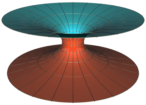
   Figure 3. Approximations [29] of parts of a catenoid and a helicoid

5. The catenoid is also induced by the Weierstrass data $\frac{1}{\,{\mathbf{G}}\,}d\mathbf{h}=\frac{1}{\,{\left({\mathbf{G}}^{2}-1\right)}^{2}\,}d{\mathbf{G}}$. It recovers the data of the Jorge-Meeks $k$-noid [14, Section 5] with $k=2$. See also [30, Section 4.4].

7. We obtain helicoids by taking conjugate minimal surfaces of catenoids. The uniqueness of the associate families of catenoids and helicoids in terms of a Chern-Ricci harmonic function is proved in [21, Theorem 3.3].

Lemma 4.2 (Chern-Ricci harmonic functions and generalization of the Chern metric).

Given a minimal surface $\Sigma$ with the Gauss curvature $\mathcal{K}$ and the Weierstrass data $\left({\mathbf{G}},d\mathbf{h}\right)$ and a finitely many distinct constant unit vector fields ${\mathbf{V}}_{1}$, $\cdots$, ${\mathbf{V}}_{N}$ and weights ${\lambda}_{1}$, $\cdots$, $\lambda_{N}\in\mathbb{Q}$ with ${\lambda}_{1}+\cdots+{\lambda}_{N}=1$, we introduce the Chern-Ricci function by the linear combination

(4.1) $$\sum_{j=1}^{N}{\lambda}_{j}\ln\frac{{\left(1+\mathbf{n}_{{}_{{\mathbf{V}}_{j}}}\right)}^{2}}{\sqrt{\,-\mathcal{K}\,}}$$

on the points where $\mathcal{K}<0$ and $1+\mathbf{n}_{{}_{{\mathbf{V}}_{j}}}>0$ for all $j\in\{1,\cdots,N\}$. Then, the Chern-Ricci function is harmonic, and the conformally changed metric

(4.2) $$\left[\prod_{j=1}^{N}{\left(1+\mathbf{n}_{{}_{{\mathbf{V}}_{j}}}\right)}^{2{\lambda}_{j}}\right]\mathbf{g}_{{}_{\Sigma}}$$

is flat. The case when $N=1$ indicates the flatness of the Chern metric (3.1) in Proposition 3.1.

Proof.

By Proposition 3.1, each component function of the Chern-Ricci function (4.1) is harmonic on $\Sigma$. Recall that the Ricci metric ${\mathbf{g}}_{{}_{\textrm{Ricci}}}=\sqrt{-{\mathcal{K}}_{{\mathbf{g}}_{{}_{\Sigma}}}}\,{\mathbf{g}}_{{}_{\Sigma}}$ is flat. Since the Chern-Ricci function (4.1) is harmonic, by the curvature formula (3.3) in Proposition 3.1, the conformally changed metric

$$\left[\prod_{j=1}^{N}{\left(1+\mathbf{n}_{{}_{{\mathbf{V}}_{j}}}\right)}^{2{\lambda}_{j}}\right]\mathbf{g}_{{}_{\Sigma}}=\prod_{j=1}^{N}\,{\left[\,\frac{{\left(1+\mathbf{n}_{{}_{{\mathbf{V}}_{j}}}\right)}^{2}}{\sqrt{\,-\mathcal{K}\,}}\,\right]}^{{\lambda}_{j}}\,{\mathbf{g}}_{{}_{\textrm{Ricci}}}$$

should be also flat. ∎

Lemma 4.3 (Chern-Ricci harmonic functions in terms of the Weierstrass data).

We identify a given constant unit vector field ${\mathbf{V}}$ by the point ${\pi}^{-1}\left(\alpha\right)\in{\mathbb{S}}^{2}$, where we denote $\pi:{\mathbb{S}}^{2}\to\overline{\,\mathbb{C}\,}$ the stereographic projection with respect to the north pole. On a negatively curved minimal surface with the Weierstrass data $\left({\mathbf{G}},d\mathbf{h}\right)$ and the unit normal vector field ${\mathbf{n}}={\pi}^{-1}\left(\mathbf{G}\right)$, the Chern-Ricci harmonic functions associated to ${\mathbf{V}}$ (see Lemma (4.2)) are given in terms of the Weierstrass data as follows.

1. (4.3) $$\ln\frac{\,{\left(1-\mathbf{n}_{{}_{\mathbf{V}}}\right)}^{2}\,}{\sqrt{-\mathcal{K}}}=\begin{cases}\ln\,\left[\;{\left(\frac{2}{\,1+{\left|\alpha\right|}^{2}\,}\right)}^{2}\left|\,\frac{{\,(\mathbf{G}-\alpha)}^{4}\,}{4\mathbf{G}}\,\frac{d\mathbf{h}}{d\mathbf{G}}\,\right|\;\right],\quad\alpha\in\overline{\,\mathbb{C}\,}-\{\infty\},\\ \\ \ln\,\left[\;{\left(\frac{2}{\,1+\frac{1}{{\left|\alpha\right|}^{2}}\,}\right)}^{2}\left|\,\frac{{\,(\frac{1}{\,\alpha\,}{\mathbf{G}}-1)}^{4}\,}{4\mathbf{G}}\,\frac{d\mathbf{h}}{d\mathbf{G}}\,\right|\;\right],\quad\alpha\in\overline{\,\mathbb{C}\,}-\{0\}.\end{cases}$$

2. (4.4) $$\ln\frac{\,{\left(1+\mathbf{n}_{{}_{\mathbf{V}}}\right)}^{2}\,}{\sqrt{-\mathcal{K}}}=\begin{cases}\ln\,\left[\;{\left(\frac{2}{\,1+{\left|\alpha\right|}^{2}\,}\right)}^{2}\left|\,\frac{{\,(\overline{\alpha}\mathbf{G}-1)}^{4}\,}{4\mathbf{G}}\,\frac{d\mathbf{h}}{d\mathbf{G}}\,\right|\;\right],\quad\alpha\in\overline{\,\mathbb{C}\,}-\{\infty\},\\ \\ \ln\,\left[\;{\left(\frac{2}{\,1+\frac{1}{{\left|\alpha\right|}^{2}}\,}\right)}^{2}\left|\,\frac{{\,({\mathbf{G}}-\frac{1}{\,\overline{\alpha}\,})}^{4}\,}{4\mathbf{G}}\,\frac{d\mathbf{h}}{d\mathbf{G}}\,\right|\;\right],\quad\alpha\in\overline{\,\mathbb{C}\,}-\{0\}.\end{cases}$$

3. (4.5) $$\ln\frac{\,{\left(1-{\mathbf{n}_{{}_{\mathbf{V}}}}^{2}\right)}\,}{\sqrt{\,-\mathcal{K}\,}}=\begin{cases}\ln\,\left[\;{\left(\frac{2\left|\alpha\right|}{\,1+{\left|\alpha\right|}^{2}\,}\right)}^{2}\left|\,\frac{{(\mathbf{G}-\alpha)}^{2}{(\mathbf{G}+\frac{1}{\,\overline{\alpha}\,})}^{2}\,}{4\mathbf{G}}\,\frac{d\mathbf{h}}{d\mathbf{G}}\,\right|\;\right],\quad\alpha\in\overline{\,\mathbb{C}\,}-\{0,\infty\},\\ \\ \ln\,\left|\,\frac{1}{\,\mathbf{G}\,}\,\frac{d\mathbf{h}}{d\mathbf{G}}\,\right|,\quad\alpha\in\{0,\infty\}.\end{cases}$$

Proof.

We first deduce the equalities in (4.3). We need to compute the Jacobi field ${\mathbf{n}}_{{}_{\mathbf{V}}}={\langle\mathbf{n},{\mathbf{V}}\rangle}_{{\mathbb{R}}^{3}}$. By the definition of the stereographic projection $\pi:{\mathbb{S}}^{2}\to\overline{\,\mathbb{C}\,}$, we have

$${\mathbf{n}}=\frac{1}{{\left|\mathbf{G}\right|}^{2}+1}\begin{bmatrix}\,2\,\textrm{Re}\left(\mathbf{G}\right)\,\\ \,2\,\textrm{Im}\left(\mathbf{G}\right)\,\\ \,{\left|\mathbf{G}\right|}^{2}-1\,\end{bmatrix}\quad\text{and}\quad{\mathbf{V}}=\frac{1}{{\left|\alpha\right|}^{2}+1}\begin{bmatrix}\,2\,\textrm{Re}\left(\alpha\right)\,\\ \,2\,\textrm{Im}\left(\alpha\right)\,\\ \,{\left|\alpha\right|}^{2}-1\,\end{bmatrix}.$$

A straightforward computation yields

(4.6) $$1-\mathbf{n}_{{}_{\mathbf{V}}}=\begin{cases}\frac{2}{\,1+{\left|\alpha\right|}^{2}\,}\frac{\,\left|{(\mathbf{G}-\alpha)}^{2}\right|\,}{1+{|\mathbf{G}|}^{2}},\quad\alpha\in\overline{\,\mathbb{C}\,}-\{\infty\},\\ \\ \frac{2}{\,1+\frac{1}{{\left|\alpha\right|}^{2}}\,}\frac{\,\left|{(\frac{1}{\alpha}{\mathbf{G}}-1)}^{2}\right|\,}{1+{|\mathbf{G}|}^{2}},\quad\alpha\in\overline{\,\mathbb{C}\,}-\{0\}.\end{cases}$$

As well-known (for instance, see [17, p. 5] and [25, Chapter 9]), the curvature ${\mathcal{K}}$ of the induced metric ${\mathbf{g}}_{{}_{\Sigma}}=\frac{1}{4}{\left(\frac{1}{\,|\mathbf{G}|\,}+|\mathbf{G}|\right)}^{2}{|d\mathbf{h}|}^{2}$ is given in terms of the Weierstrass data:

(4.7) $$\sqrt{-{\mathcal{K}}\,}=\sqrt{-{\mathcal{K}}_{{\mathbf{g}}_{{}_{\Sigma}}}\,}={\left(\frac{2}{\;\frac{1}{\,|\mathbf{G}|\,}+|\mathbf{G}|\;}\right)}^{2}\left|\,\frac{1}{\,\mathbf{G}\frac{\,d\mathbf{h}\,}{\,d\mathbf{G}\,}\,}\,\right|.$$

Combining (4.6) and (4.7) gives the equalities in (4.3). Replacing the pair $\left({\mathbf{V}},\alpha\right)$ in (4.3) by $\left(-{\mathbf{V}},\frac{1}{\,\overline{\alpha}\,}\right)$ and observing the identity $\mathbf{n}_{{}_{-\mathbf{V}}}=-\mathbf{n}_{{}_{\mathbf{V}}}$ yield the equalities in (4.4). Adding the equalities in (4.3) and (4.4) gives the equalities in (4.5). ∎

5. Classifications of minimal surfaces with constant Chern-Ricci functions

We classify minimal surfaces in terms of Chern-Ricci harmonic functions, and examine the limit behaviors of periodic minimal surfaces.

Theorem 5.1 (Rigidity of the associate family of Scherk’s surfaces).

Given a minimal surface with the Gauss curvature $\mathcal{K}<0$ and the unit normal $\mathbf{n}$, if there exists two orthogonal constant unit vector fields ${\mathbf{V}}_{1}$ and ${\mathbf{V}}_{2}$ such that the Chern-Ricci harmonic function (introduced in Lemma 4.2)

(5.1) $$\sum_{\mathbf{V}\in\left\{{\mathbf{V}}_{1},-{\mathbf{V}}_{1},{\mathbf{V}}_{2},-{\mathbf{V}}_{2}\right\}}\ln\frac{\,{\left(1-{\mathbf{n}}_{{}_{{\mathbf{V}}}}\right)}^{2}\,}{\sqrt{\,-{\mathcal{K}}}\,}$$

is constant, then the minimal surface should be congruent to (a part of) a member of the associate family connecting a doubly periodic Scherk graph and a singly periodic Scherk tower (up to homotheties).

Proof.

Without loss of generality, after applying rotations, we could take the identifications

$${\mathbf{V}}_{1}=\begin{bmatrix}\,1\,\\ \,0\,\\ \,0\,\end{bmatrix}={\pi}^{-1}\left(1\right),\;\;-{\mathbf{V}}_{1}=\begin{bmatrix}\,-1\,\\ \,0\,\\ \,0\,\end{bmatrix}={\pi}^{-1}\left(-1\right),\;\;{\mathbf{V}}_{2}=\begin{bmatrix}\,0\,\\ \,1\,\\ \,0\,\end{bmatrix}={\pi}^{-1}\left(i\right),\;\;-{\mathbf{V}}_{2}=\begin{bmatrix}\,0\,\\ \,-1\,\\ \,0\,\end{bmatrix}={\pi}^{-1}\left(-i\right).$$

Here, recall that $\pi:{\mathbb{S}}^{2}\to\overline{\,\mathbb{C}\,}$ denotes the stereographic projection from the north pole. Let $\left({\mathbf{G}},d\mathbf{h}\right)$ denote the Weierstrass data. We use the formula (4.3) in Lemma 4.3

$$\ln\frac{\,{\left(1-\mathbf{n}_{{}_{\mathbf{V}}}\right)}^{2}\,}{\sqrt{-\mathcal{K}}}=\ln\,\left[\;{\left(\frac{2}{\,1+{\left|\alpha\right|}^{2}\,}\right)}^{2}\left|\,\frac{{\,(\mathbf{G}-\alpha)}^{4}\,}{4\mathbf{G}}\,\frac{d\mathbf{h}}{\,d\mathbf{G}\,}\,\right|\;\right]$$

for $\alpha\in\{1,-1,i,-1\}$. The constancy of the function (5.1) guarantees that the product function

$$\left|\,\frac{1}{{\mathbf{G}}^{4}}{\left(\frac{d\mathbf{h}}{\,d\mathbf{G}\,}\right)}^{4}\,\prod_{\alpha\in\{1,-1,i,-1\}}(\mathbf{G}-\alpha)^{4}\right|\,={\left|\,\frac{1}{{\mathbf{G}}}\frac{d\mathbf{h}}{\,d\mathbf{G}\,}\,({\mathbf{G}}^{4}-1)\right|}^{4}\,$$

is a positive constant. Hence, there exist constants $\rho>0$ and $\Theta\in\left[0,2\pi\right]$ such that

$$\frac{1}{{\mathbf{G}}}{d\mathbf{h}}=\frac{\rho\,{e}^{i\Theta}}{{\mathbf{G}}^{4}-1}{d\mathbf{G}}.$$

∎

Remark 5.2 (Rigidity of Scherk’s surfaces in terms of two flat structures).

We first explain that Theorem 5.1 is equivalent to Theorem 2.1. Indeed, taking account into the identity $\mathbf{n}_{{}_{-\mathbf{V}}}=-\mathbf{n}_{{}_{\mathbf{V}}}$ and letting $\mathcal{V}:=\left\{{\mathbf{V}}_{1},-{\mathbf{V}}_{1},{\mathbf{V}}_{2},-{\mathbf{V}}_{2}\right\}$, we have

$$\sum_{\mathbf{V}\in\mathcal{V}}\ln\frac{\,{\left(1-{\mathbf{n}}_{{}_{{\mathbf{V}}}}\right)}^{2}\,}{\sqrt{\,-{\mathcal{K}}}\,}=\sum_{\mathbf{V}\in\mathcal{V}}\ln\frac{\,{\left(1+{\mathbf{n}}_{{}_{{\mathbf{V}}}}\right)}^{2}\,}{\sqrt{\,-{\mathcal{K}}}\,}=2\sum_{\mathbf{V}\in\left\{{\mathbf{V}}_{1},{\mathbf{V}}_{2}\right\}}\ln\frac{\,1-{{\mathbf{n}}_{{}_{{\mathbf{V}}}}}^{2}\,}{\sqrt{\,-{\mathcal{K}}}\,}=4\ln\frac{\,\sqrt{\left(1-{{\mathbf{n}}_{{}_{{{\mathbf{V}}_{1}}}}}^{2}\right)\left(1-{{\mathbf{n}}_{{}_{{{\mathbf{V}}_{2}}}}}^{2}\right)}\,}{\sqrt{\,-{\mathcal{K}}}\,}.$$

Theorem 5.1 shows that, on a minimal surface, the flat metric

$$\sqrt{\left(1-{{\mathbf{n}}_{{}_{{{\mathbf{V}}_{1}}}}}^{2}\right)\left(1-{{\mathbf{n}}_{{}_{{{\mathbf{V}}_{2}}}}}^{2}\right)}\,{\mathbf{g}}_{{}_{\Sigma}}$$

could become a constant multiple of the flat metric ${\mathbf{g}}_{{}_{\textrm{Ricci}}}=\sqrt{-{\mathcal{K}}_{{\mathbf{g}}_{{}_{\Sigma}}}}\,{\mathbf{g}}_{{}_{\Sigma}}$, only when it belongs to the associate family of Scherk’s surfaces.

Figure 4. An approximation [29] of a part of a sheared singly periodic Scherk’s surface

Theorem 5.3 (Rigidity of the associate family of generalized Scherk’s surfaces).

Given a minimal surface with the Gauss curvature $\mathcal{K}<0$ and the unit normal $\mathbf{n}$, if there exists two distinct unit vector fields ${\mathbf{V}}_{1}$ and ${\mathbf{V}}_{2}$ such that the Chern-Ricci harmonic function

(5.2) $$\sum_{\mathbf{V}\in\left\{{\mathbf{V}}_{1},-{\mathbf{V}}_{1},{\mathbf{V}}_{2},-{\mathbf{V}}_{2}\right\}}\ln\frac{\,{\left(1-{\mathbf{n}}_{{}_{{\mathbf{V}}}}\right)}^{2}\,}{\sqrt{\,-{\mathcal{K}}}\,}$$

is constant, then the minimal surface should be congruent to (a part of) a member of the associate family connecting a generalized doubly periodic Scherk graph and a generalized singly periodic Scherk tower.

Proof.

Without loss of generality, after applying rotations, we could take the identifications

$${\mathbf{V}}_{1}={\pi}^{-1}\left(e^{i\theta}\right),\;\;-{\mathbf{V}}_{1}={\pi}^{-1}\left(-e^{i\theta}\right),\;\;{\mathbf{V}}_{2}={\pi}^{-1}\left(e^{-i\theta}\right),\;\;-{\mathbf{V}}_{2}={\pi}^{-1}\left(-e^{-i\theta}\right),$$

where $\pi:{\mathbb{S}}^{2}\to\overline{\,\mathbb{C}\,}$ is the stereographic projection. We use the formula (4.3) in Lemma 4.3

$$\ln\frac{\,{\left(1-\mathbf{n}_{{}_{\mathbf{V}}}\right)}^{2}\,}{\sqrt{-\mathcal{K}}}=\ln\,\left[\;{\left(\frac{2}{\,1+{\left|\alpha\right|}^{2}\,}\right)}^{2}\left|\,\frac{{\,(\mathbf{G}-\alpha)}^{4}\,}{4\mathbf{G}}\,\frac{d\mathbf{h}}{\,d\mathbf{G}\,}\,\right|\;\right]$$

for $\alpha\in\{e^{i\theta},-e^{i\theta},e^{-i\theta},-e^{-i\theta}\}$. The constancy of the function (5.2) guarantees that the product

$$\left|\,\frac{1}{{\mathbf{G}}^{4}}{\left(\frac{d\mathbf{h}}{\,d\mathbf{G}\,}\right)}^{4}\,\prod_{\alpha\in\{e^{i\theta},-e^{i\theta},e^{-i\theta},-e^{-i\theta}\}}(\mathbf{G}-\alpha)^{4}\right|\,={\left|\,\frac{1}{{\mathbf{G}}}\frac{d\mathbf{h}}{\,d\mathbf{G}\,}\,\left({\mathbf{G}}^{2}-{e^{2i\theta}}\right)\left({\mathbf{G}}^{2}-{e^{-2i\theta}}\right)\right|}^{4}\,$$

is a positive constant. We recover the Weierstrass data for the associate family of generalized Scherk’s surfaces [6, 15, 30]:

$$\frac{1}{{\mathbf{G}}}{d\mathbf{h}}=\frac{\rho\,{e}^{i\Theta}}{\,\left({\mathbf{G}}^{2}-{e^{2i\theta}}\right)\left({\mathbf{G}}^{2}-{e^{-2i\theta}}\right)\,}{d\mathbf{G}}$$

for some constants $\rho>0$ and $\Theta\in\left[0,2\pi\right]$. ∎

Example 5.4 (triply periodic tCLP surfaces connecting doubly periodic Scherk surfaces and singly periodic Scherk surfaces).

Imagine eight points on the unit circle ${\mathbb{S}}^{1}$ in the $xy$-plane:

(5.3) $$\pm{\mathbf{V}}_{1}=\pm\begin{bmatrix}\,\cos\theta\,\\ \,\sin\theta\,\\ \,0\,\end{bmatrix},\;\;\pm{\mathbf{V}}_{2}=\pm\begin{bmatrix}\,\sin\theta\,\\ \,\cos\theta\,\\ \,0\,\end{bmatrix},\;\;\pm{\mathbf{V}}_{3}=\pm\begin{bmatrix}\,-\sin\theta\,\\ \,\cos\theta\,\\ \,0\,\end{bmatrix},\;\;\pm{\mathbf{V}}_{4}=\pm\begin{bmatrix}\,-\cos\theta\,\\ \,\sin\theta\,\\ \,0\,\end{bmatrix}.$$

For $\theta\in\left(0,\frac{\pi}{4}\right)$, after identifying these eight vertices in ${\mathbb{S}}^{1}\subset{\mathbb{S}}^{2}\subset{\mathbb{R}}^{3}$ as the constant unit vector fields, we want to construct minimal surfaces so that the Chern-Ricci harmonic function

(5.4) $$\sum_{\mathbf{V}\in\left\{\pm{\mathbf{V}}_{1},\pm{\mathbf{V}}_{2},\pm{\mathbf{V}}_{3},\pm{\mathbf{V}}_{4}\right\}}\ln\frac{\,{\left(1-{\mathbf{n}}_{{}_{{\mathbf{V}}}}\right)}^{2}\,}{\sqrt{\,-{\mathcal{K}}}\,}$$

is constant. When $\theta\mathrel{\text{\rotatebox[origin={c}]{315.0}{$\vrule height=0.0pt,width=0.0pt\shortrightarrow$}}}0$ or $\theta\mathrel{\text{\rotatebox[origin={c}]{45.0}{$\vrule height=0.0pt,width=0.0pt\shortrightarrow$}}}\frac{\pi}{4}$, can we geometrically prescribe the limit minimal surfaces? We observe that the eight vertices consist of two congruent rectangles in the $xy$-plane.

1. When $\theta\mathrel{\text{\rotatebox[origin={c}]{315.0}{$\vrule height=0.0pt,width=0.0pt\shortrightarrow$}}}0$, two congruent rectangles collapses to the union of two orthogonal segments. We expect that the limit surfaces has the constant Chern-Ricci harmonic function

   (5.5) $$\sum_{\mathbf{V}\in\left\{\pm{\left(1,0,0\right)}^{\intercal},\,\pm{\left(0,1,0\right)}^{\intercal}\right\}}\ln\frac{\,{\left(1-{\mathbf{n}}_{{}_{{\mathbf{V}}}}\right)}^{2}\,}{\sqrt{\,-{\mathcal{K}}}\,}.$$

2. When $\theta\mathrel{\text{\rotatebox[origin={c}]{45.0}{$\vrule height=0.0pt,width=0.0pt\shortrightarrow$}}}\frac{\pi}{4}$, two congruent rectangles collapses to the union of the orthogonal segments. We expect that the limit surfaces has the constant Chern-Ricci harmonic function

   (5.6) $$\sum_{\mathbf{V}\in\left\{\pm{\left(\cos\left(\frac{\pi}{4}\right),\sin\left(\frac{\pi}{4}\right),0\right)}^{\intercal},\,\pm{\left(\cos\left(\frac{3\pi}{4}\right),\sin\left(\frac{3\pi}{4}\right),0\right)}^{\intercal}\right\}}\ln\frac{\,{\left(1-{\mathbf{n}}_{{}_{{\mathbf{V}}}}\right)}^{2}\,}{\sqrt{\,-{\mathcal{K}}}\,}.$$

Theorem 5.1 guarantees that such limit surfaces are members of the associate family from a doubly periodic Scherk surface to a singly periodic Scherk surface. We find minimal surfaces with a constant Chern-Ricci harmonic function in (5.4). For $\theta\in\left(0,\frac{\pi}{4}\right)$, we have the image

$$\mathcal{A}:={\pi}\left(\,\left\{\pm{\mathbf{V}}_{1},\pm{\mathbf{V}}_{2},\pm{\mathbf{V}}_{3},\pm{\mathbf{V}}_{4}\right\}\,\right)=\left\{\,\pm e^{i\theta},\,\pm ie^{i\theta},\,\pm e^{-i\theta},\,\pm ie^{-i\theta}\,\right\},$$

where $\pi:{\mathbb{S}}^{2}\to\overline{\,\mathbb{C}\,}$ is the stereographic projection. According to the formula (4.3) in Lemma 4.3

$$\ln\frac{\,{\left(1-\mathbf{n}_{{}_{\mathbf{V}}}\right)}^{2}\,}{\sqrt{-\mathcal{K}}}=\ln\,\left[\;{\left(\frac{2}{\,1+{\left|\alpha\right|}^{2}\,}\right)}^{2}\left|\,\frac{{\,(\mathbf{G}-\alpha)}^{4}\,}{4\mathbf{G}}\,\frac{d\mathbf{h}}{\,d\mathbf{G}\,}\,\right|\;\right],$$

we see that the constancy of the prescribed Chern-Ricci function (5.4) implies that constancy of

$$\left|\,\frac{1}{{\mathbf{G}}^{8}}{\left(\frac{d\mathbf{h}}{\,d\mathbf{G}\,}\right)}^{8}\,{\left({\mathbf{G}}^{2}-{e}^{2i\theta}\right)}^{4}{\left({\mathbf{G}}^{2}+{e}^{2i\theta}\right)}^{4}{\left({\mathbf{G}}^{2}-{e}^{-2i\theta}\right)}^{4}{\left({\mathbf{G}}^{2}+{e}^{-2i\theta}\right)}^{4}\,\right|.$$

This recovers, up to associate families, the triply periodic minimal surface ${\Sigma}_{\lambda\in\left(-2,2\right)}$ in tCLP family [7, 18] with the Weierstrass data

$$\frac{1}{{\mathbf{G}}}{d\mathbf{h}}=\frac{1}{\,\sqrt{{\mathbf{G}}^{8}+\lambda{\mathbf{G}}^{4}+1}\,}d{\mathbf{G}\,},\quad\lambda=-2\cos\left(4\theta\right)\in\left(-2,2\right).$$

1. The limit surface ${\Sigma}_{-2}$ recovers the doubly periodic Scherk surface with

   $$\frac{1}{{\mathbf{G}}}{d\mathbf{h}}=\frac{1}{\,{\mathbf{G}}^{4}-1\,}d{\mathbf{G}\,}.$$

2. The limit surface ${\Sigma}_{2}$ recovers the singly periodic Scherk surface with

   $$\frac{1}{{\mathbf{G}}}{d\mathbf{h}}=\frac{1}{\,{\mathbf{G}}^{4}+1\,}d{\mathbf{G}\,}.$$

Example 5.5 (From triply periodic Schwarz D surface to doubly periodic Scherk surface).

Imagine a cube inscribed in the round unit sphere ${\mathbb{S}}^{2}$ sitting in ${\mathbb{R}}^{3}$. The side length of the cube is $\sqrt{\frac{4}{3}}$. Taking $\theta={\sin}^{-1}\left(\,\sqrt{{\frac{1}{3}}}\,\right)$, we obtain an example of such cube with the vertices in ${\mathbb{S}}^{2}$:

(5.7) $$\pm{\mathbf{V}}_{1}=\pm\begin{bmatrix}\,\cos\theta\,\\ \,0\,\\ \,\sin\theta\,\end{bmatrix},\;\;\pm{\mathbf{V}}_{2}=\pm\begin{bmatrix}\,\cos\theta\,\\ \,0\,\\ \,-\sin\theta\,\end{bmatrix},\;\;\pm{\mathbf{V}}_{3}=\pm\begin{bmatrix}\,0\,\\ \,\cos\theta\,\\ \,\sin\theta\,\end{bmatrix},\;\;\pm{\mathbf{V}}_{4}=\pm\begin{bmatrix}\,0\,\\ \,\cos\theta\,\\ \,-\sin\theta\,\end{bmatrix}.$$

For $\theta\in\left(0,\frac{\pi}{2}\right)$, after identifying these eight vertices in ${\mathbb{S}}^{2}$ as the constant unit vector fields, we want to construct minimal surfaces so that the Chern-Ricci harmonic function

(5.8) $$\sum_{\mathbf{V}\in\left\{\pm{\mathbf{V}}_{1},\pm{\mathbf{V}}_{2},\pm{\mathbf{V}}_{3},\pm{\mathbf{V}}_{4}\right\}}\ln\frac{\,{\left(1-{\mathbf{n}}_{{}_{{\mathbf{V}}}}\right)}^{2}\,}{\sqrt{\,-{\mathcal{K}}}\,}$$

is constant. For $\theta\in\left(0,\frac{\pi}{2}\right)$, taking $a=\tan\left(\frac{\pi}{4}-\frac{\theta}{2}\right)$, we have the image

$$\mathcal{A}:={\pi}\left(\,\left\{\pm{\mathbf{V}}_{1},\pm{\mathbf{V}}_{2},\pm{\mathbf{V}}_{3},\pm{\mathbf{V}}_{4}\right\}\,\right)=\left\{a,-\frac{1}{a},ai,-\frac{1}{\,\overline{ai}}=\frac{i}{a},-a,\frac{1}{a},-ai,-\frac{1}{\,\overline{-ai}}=-\frac{i}{a}\,\right\},$$

where $\pi:{\mathbb{S}}^{2}\to\overline{\,\mathbb{C}\,}$ is the stereographic projection. According to the formula (4.3) in Lemma 4.3

$$\ln\frac{\,{\left(1-\mathbf{n}_{{}_{\mathbf{V}}}\right)}^{2}\,}{\sqrt{-\mathcal{K}}}=\ln\,\left[\;{\left(\frac{2}{\,1+{\left|\alpha\right|}^{2}\,}\right)}^{2}\left|\,\frac{{\,(\mathbf{G}-\alpha)}^{4}\,}{4\mathbf{G}}\,\frac{d\mathbf{h}}{\,d\mathbf{G}\,}\,\right|\;\right],$$

we see that the constancy of the prescribed Chern-Ricci function (5.4) implies that constancy of

$$\left|\,\frac{1}{{\mathbf{G}}^{8}}{\left(\frac{d\mathbf{h}}{\,d\mathbf{G}\,}\right)}^{8}\,{\left({\mathbf{G}}^{4}-{a}^{4}\right)}^{4}{\left({\mathbf{G}}^{4}-\frac{1}{{a}^{4}}\right)}^{4}\,\right|.$$

This recovers the triply periodic minimal surface ${\Sigma}_{\lambda\in\left(-\infty,-2\right)}$ in tD family determined by

$$\frac{1}{{\mathbf{G}}}{d\mathbf{h}}=\frac{1}{\,\sqrt{{\mathbf{G}}^{8}+\lambda{\mathbf{G}}^{4}+1}\,}d{\mathbf{G}\,},$$

up to associate families (and homotheties). It is straightforward to check that

$$\lambda=-\left({a}^{4}+\frac{1}{{a}^{4}}\right)=2-{\left[\,a^{2}+\frac{1}{a^{2}}\,\right]}^{2}=-2-16\frac{{\sin}^{2}\theta}{{\cos}^{4}\theta}<-2.$$

1. For $\theta={\sin}^{-1}\left(\,\sqrt{{\frac{1}{3}}}\,\right)$, we find that the eight vertices in (5.7) consist of a cube inscribed in the unit sphere, and meet Schwarz diamond surface ${\Sigma}_{-14}$.

2. The limit surface ${\Sigma}_{-2}$ is the doubly periodic Scherk surface with the Weierstrass data

   $$\frac{1}{{\mathbf{G}}}{d\mathbf{h}}=\frac{1}{\,{\mathbf{G}}^{4}-1\,}d{\mathbf{G}\,}.$$

Figure 5. Approximations [29] of parts of triply periodic Schwarz D and P surfaces

Example 5.6 (From triply periodic Schwarz P surface to singly periodic Scherk tower).

The triply periodic minimal surface ${\Sigma}_{\lambda\in\left(2,\infty\right)}$ in tP family admits the Weierstrass data

$$\frac{1}{{\mathbf{G}}}{d\mathbf{h}}=\frac{1}{\,\sqrt{{\mathbf{G}}^{8}+\lambda{\mathbf{G}}^{4}+1}\,}d{\mathbf{G}\,}.$$

1. ${\Sigma}_{14}$ becomes the Schwarz primitive surface.

2. The limit surface ${\Sigma}_{2}$ induces the singly periodic Scherk tower with the Weierstrass data

   $$\frac{1}{{\mathbf{G}}}{d\mathbf{h}}=\frac{1}{\,{\mathbf{G}}^{4}+1\,}d{\mathbf{G}\,}.$$

Remark 5.7.

Meeks’ family [24, p. 912] includes minimal surfaces in Example 5.4, 5.5, 5.6.

Proposition 5.8 (Conjugate surfaces of minimal surfaces in Example 5.4, 5.5, 5.6).

Let ${\Sigma}_{\lambda\in\mathbb{R}}$ denote the minimal surface with the Weierstrass data

$${d\mathbf{h}}=\frac{{\mathbf{G}}}{\,\sqrt{{\mathbf{G}}^{8}+\lambda{\mathbf{G}}^{4}+1}\,}d{\mathbf{G}\,}.$$

Then, the conjugate minimal surface of ${\Sigma}_{\lambda}$ is congruent to the minimal surface ${\Sigma}_{-\lambda}$. See also [18, Example 6.3]. In particular, the Schwarz CLP surface ${\Sigma}_{0}$ [8, 16, 27] is self-conjugate. The Schwarz P surface ${\Sigma}_{14}$ in the tP family is conjugate to the Schwarz D surface ${\Sigma}_{-14}$ in the tD family.

Proof.

Since $\left(e^{i\frac{\pi}{4}}\right)^{2}=i$, $\left(e^{i\frac{\pi}{4}}\right)^{4}=-1$, and $\left(e^{i\frac{\pi}{4}}\right)^{8}=1$, the rotated Gauss map $\widetilde{\,\mathbf{G}\,}:=e^{i\frac{\pi}{4}}\mathbf{G}$ solves

$$\frac{i\,{\mathbf{G}}}{\,\sqrt{{\mathbf{G}}^{8}+\lambda{\mathbf{G}}^{4}+1}\,}d{\mathbf{G}\,}=\frac{\widetilde{\,\mathbf{G}\,}}{\,\sqrt{{{\,\widetilde{\,\mathbf{G}\,}\,}}^{8}-\lambda{{\,\widetilde{\,\mathbf{G}\,}\,}}^{4}+1}\,}d{{\widetilde{\,\mathbf{G}\,}\,}}.$$

∎

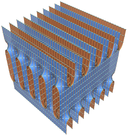
Figure 6. Approximations [29] of parts of triply periodic Schwarz CLP surfaces

Example 5.9 (rPD family containing both Schwarz P surface and Schwarz D surface).

Imagine a regular tetrahedron inscribed in the round unit sphere ${\mathbb{S}}^{2}$ sitting in ${\mathbb{R}}^{3}$. The side length of the regular tetrahedron is $\sqrt{\frac{8}{3}}$. Taking $\theta={\sin}^{-1}\left(\,{\frac{1}{3}}\,\right)$, we obtain an example of such regular tetrahedron with the following vertices in ${\mathbb{S}}^{2}$:

(5.9) $${\mathbf{V}}_{0}=\begin{bmatrix}\,0\,\\ \,0\,\\ \,1\,\end{bmatrix},\;\;{\mathbf{V}}_{1}=\begin{bmatrix}\,\cos\theta\,\\ \,0\,\\ \,-\sin\theta\,\end{bmatrix},\;\;{\mathbf{V}}_{2}=\begin{bmatrix}\,\cos\theta\cos\left(\frac{2\pi}{3}\right)\,\\ \,\cos\theta\sin\left(\frac{2\pi}{3}\right)\,\\ \,-\sin\theta\,\end{bmatrix},\;\;{\mathbf{V}}_{3}=\begin{bmatrix}\,\cos\theta\cos\left(-\frac{2\pi}{3}\right)\,\\ \,\cos\theta\sin\left(-\frac{2\pi}{3}\right)\,\\ \,-\sin\theta\,\end{bmatrix}.$$

For $\theta\in\left(-\frac{\pi}{2},\frac{\pi}{2}\right)$, after identifying the 8 points $\pm{\mathbf{V}}_{0},\pm{\mathbf{V}}_{1},\pm{\mathbf{V}}_{2},\pm{\mathbf{V}}_{3}$ in ${\mathbb{S}}^{2}$ as the constant unit vector fields, we construct minimal surfaces such that the Chern-Ricci harmonic function

(5.10) $$\sum_{\mathbf{V}\in\left\{\pm{\mathbf{V}}_{0},\pm{\mathbf{V}}_{1},\pm{\mathbf{V}}_{2},\pm{\mathbf{V}}_{3}\right\}}\ln\frac{\,{\left(1-{\mathbf{n}}_{{}_{{\mathbf{V}}}}\right)}^{2}\,}{\sqrt{\,-{\mathcal{K}}}\,}$$

is constant. Taking $a=\tan\left(\frac{\pi}{4}-\frac{\theta}{2}\right)$ and $\omega=e^{i\frac{2\pi}{3}}$, we have the image

$$\mathcal{A}:={\pi}\left(\,\left\{\pm{\mathbf{V}}_{0},\pm{\mathbf{V}}_{1},\pm{\mathbf{V}}_{2},\pm{\mathbf{V}}_{3}\right\}\,\right)=\left\{\infty,a,a{\omega},a{{\omega}^{2}},0,-\frac{1}{a},-\frac{1}{a}{\omega},-\frac{1}{a}{\omega}^{2}\,\right\},$$

where $\pi:{\mathbb{S}}^{2}\to\overline{\,\mathbb{C}\,}$ denotes the stereographic projection from the north pole. To determine the Weierstrass data of desired minimal surfaces, we shall use the formula (4.3) in Lemma 4.3

$$\ln\frac{\,{\left(1-\mathbf{n}_{{}_{\mathbf{V}}}\right)}^{2}\,}{\sqrt{-\mathcal{K}}}=\begin{cases}\ln\,\left|\;{\mathbf{G}}^{3}\frac{d\mathbf{h}}{d\mathbf{G}}\;\right|,\quad\alpha=0,\\ \ln\,\left[\;{\left(\frac{2}{\,1+{\left|\alpha\right|}^{2}\,}\right)}^{2}\left|\,\frac{{\,(\mathbf{G}-\alpha)}^{4}\,}{4\mathbf{G}}\,\frac{d\mathbf{h}}{d\mathbf{G}}\,\right|\;\right],\quad\alpha\in\overline{\,\mathbb{C}\,}-\{0,\infty\},\\ \ln\,\left|\;\frac{1}{\mathbf{G}}\frac{d\mathbf{h}}{d\mathbf{G}}\;\right|,\quad\alpha=\infty.\end{cases}$$

We see that the constancy of the prescribed Chern-Ricci function (5.10) implies that constancy of

$$\left|\,\frac{1}{{\mathbf{G}}^{4}}\,{\left({\mathbf{G}}^{3}-{a}^{3}\right)}^{4}{\left({\mathbf{G}}^{3}+\frac{1}{a^{3}}\right)}^{4}\,{\left(\frac{d\mathbf{h}}{\,d\mathbf{G}\,}\right)}^{8}\,\right|.$$

This recovers, up to associate families, the triply periodic minimal surface ${\Sigma}_{a>0}$ in the rPD family [10, 11, 27] with the Weierstrass data

$$\frac{1}{{\mathbf{G}}}{d\mathbf{h}}=\frac{1}{\,\sqrt{{\mathbf{G}}{\left({\mathbf{G}}^{3}-{a}^{3}\right)}{\left({\mathbf{G}}^{3}+\frac{1}{a^{3}}\right)}}\,}d{\mathbf{G}\,},\quad a>0.$$

1. The conjugate surface of the minimal surface ${\Sigma}_{a}$ is congruent to ${\Sigma}_{\frac{1}{a}}$. In particular, the minimal surface ${\Sigma}_{1}$ is self-conjugate.

2. When $a=\frac{1}{\sqrt{2}}$, we have $\theta={\sin}^{-1}\left(\,{\frac{1}{3}}\,\right)$. The eight vertices

   $$\pm{\mathbf{V}}_{0},\pm{\mathbf{V}}_{1},\pm{\mathbf{V}}_{2},\pm{\mathbf{V}}_{3}$$

   consists of a cube inscribed in ${\mathbb{S}}^{2}$. The surface ${\Sigma}_{\frac{1}{\sqrt{2}}}$ is the Schwarz P surface.

3. When $a=\sqrt{2}$, we have $\theta={\sin}^{-1}\left(\,-{\frac{1}{3}}\,\right)$. The eight vertices

   $$\pm{\mathbf{V}}_{0},\pm{\mathbf{V}}_{1},\pm{\mathbf{V}}_{2},\pm{\mathbf{V}}_{3}$$

   consists of a cube inscribed in ${\mathbb{S}}^{2}$. The surface ${\Sigma}_{\sqrt{2}}$ is the Schwarz D surface.

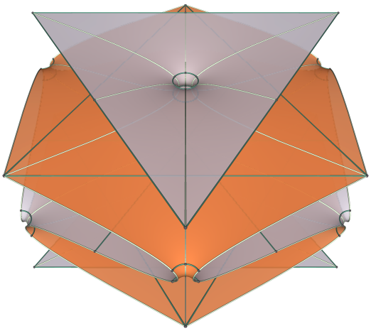
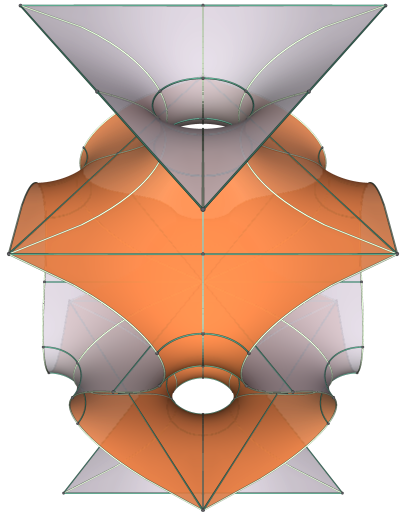
Figure 7. Approximations [29] of parts of triply periodic Schwarz rPD surfaces

Example 5.10 (Karcher’s saddle tower with 6 ends as the limit of surfaces in hCLP surfaces).

Fix the angle $\theta\in\left(0,\frac{\pi}{3}\right)$. Identifying the following eight points in ${\mathbb{S}}^{2}$

(5.11) $${\mathbf{V}}_{1}=\begin{bmatrix}\,\cos\theta\,\\ \,\sin\theta\,\\ \,0\,\end{bmatrix},\;\;{\mathbf{V}}_{2}=\begin{bmatrix}\,\cos\left(\theta+\frac{2\pi}{3}\right)\,\\ \,\sin\left(\theta+\frac{2\pi}{3}\right)\,\\ \,0\,\end{bmatrix},\;\;{\mathbf{V}}_{3}=\begin{bmatrix}\,\cos\left(\theta+\frac{4\pi}{3}\right)\,\\ \,\sin\left(\theta+\frac{4\pi}{3}\right)\,\\ \,0\,\end{bmatrix},{\mathbf{V}}_{4}=\begin{bmatrix}\,0\,\\ \,0\,\\ \,1\,\end{bmatrix},\;\;$$

(5.12) $${\mathbf{V}}_{5}=\begin{bmatrix}\,\cos\left(-\theta\right)\,\\ \,\sin\left(-\theta\right)\,\\ \,0\,\end{bmatrix},\;\;{\mathbf{V}}_{6}=\begin{bmatrix}\,\cos\left(-\theta+\frac{2\pi}{3}\right)\,\\ \,\sin\left(-\theta+\frac{2\pi}{3}\right)\,\\ \,0\,\end{bmatrix},\;\;{\mathbf{V}}_{7}=\begin{bmatrix}\,\cos\left(-\theta+\frac{4\pi}{3}\right)\,\\ \,\sin\left(-\theta+\frac{4\pi}{3}\right)\,\\ \,0\,\end{bmatrix},{\mathbf{V}}_{8}=\begin{bmatrix}\,0\,\\ \,0\,\\ \,-1\,\end{bmatrix},\;\;$$

as the constant unit vector fields, we find minimal surfaces such that the Chern-Ricci function

(5.13) $$\sum_{\mathbf{V}\in\left\{{\mathbf{V}}_{1},\cdots,{\mathbf{V}}_{8}\right\}}\ln\frac{\,{\left(1-{\mathbf{n}}_{{}_{{\mathbf{V}}}}\right)}^{2}\,}{\sqrt{\,-{\mathcal{K}}}\,}$$

is constant. It recovers the triply periodic hCLP surface [8, 9] with the Weierstrass data

$$\frac{1}{{\mathbf{G}}}{d\mathbf{h}}=\frac{1}{\,\sqrt{{\mathbf{G}}{\left({\mathbf{G}}^{6}-2\cos\left(3\theta\right){\mathbf{G}}^{3}+1\right)}}\,}d{\mathbf{G}\,},\quad\theta\in\left(0,\frac{\pi}{3}\right),$$

up to associate families. As known in [8, Theorem 1.2], when $\theta\mathrel{\text{\rotatebox[origin={c}]{45.0}{$\vrule height=0.0pt,width=0.0pt\shortrightarrow$}}}\frac{\pi}{3}$, we recover Karcher’s saddle tower with 6 ends [15].

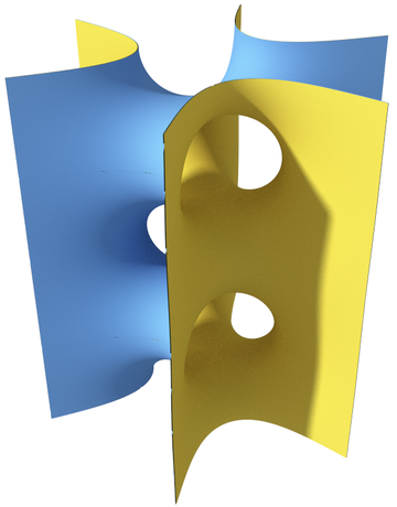
Figure 8. An approximation [32] of a part of Karcher’s saddle tower with 6 ends [15]

Example 5.11 (Karcher’s saddle tower with 6 ends as the limit of Schwarz surfaces in H family).

Fix the angle $\theta\in\left(0,\frac{\pi}{2}\right)$. Identifying the following eight points in ${\mathbb{S}}^{2}$

(5.14) $${\mathbf{V}}_{1}=\begin{bmatrix}\,-\cos\theta\,\\ \,0\,\\ \,\sin\theta\,\end{bmatrix},\;\,{\mathbf{V}}_{2}=\begin{bmatrix}\,-\cos\theta\cos\left(\frac{2\pi}{3}\right)\,\\ \,-\cos\theta\sin\left(\frac{2\pi}{3}\right)\,\\ \,\sin\theta\,\end{bmatrix},\;\,{\mathbf{V}}_{3}=\begin{bmatrix}\,-\cos\theta\cos\left(\frac{4\pi}{3}\right)\,\\ \,-\cos\theta\sin\left(\frac{4\pi}{3}\right)\,\\ \,\sin\theta\,\end{bmatrix},\;\,{\mathbf{V}}_{4}=\begin{bmatrix}\,0\,\\ \,0\,\\ \,1\,\end{bmatrix},\;\,$$

(5.15) $${\mathbf{V}}_{5}=\begin{bmatrix}\,-\cos\theta\,\\ \,0\,\\ \,-\sin\theta\,\end{bmatrix},\;\,{\mathbf{V}}_{6}=\begin{bmatrix}\,-\cos\theta\cos\left(\frac{2\pi}{3}\right)\,\\ \,-\cos\theta\sin\left(\frac{2\pi}{3}\right)\,\\ \,-\sin\theta\,\end{bmatrix},\;\,{\mathbf{V}}_{7}=\begin{bmatrix}\,-\cos\theta\cos\left(\frac{4\pi}{3}\right)\,\\ \,-\cos\theta\sin\left(\frac{4\pi}{3}\right)\,\\ \,-\sin\theta\,\end{bmatrix},\;\,{\mathbf{V}}_{8}=\begin{bmatrix}\,0\,\\ \,0\,\\ \,-1\,\end{bmatrix},\;\;$$

as the constant unit vector fields, we find minimal surfaces such that the Chern-Ricci function

(5.16) $$\sum_{\mathbf{V}\in\left\{{\mathbf{V}}_{1},\cdots,{\mathbf{V}}_{8}\right\}}\ln\frac{\,{\left(1-{\mathbf{n}}_{{}_{{\mathbf{V}}}}\right)}^{2}\,}{\sqrt{\,-{\mathcal{K}}}\,}$$

is constant. Take $a=\tan\left(\frac{\pi}{4}-\frac{\theta}{2}\right)\in\left(0,1\right)$. It recovers, up to associate families, the triply periodic minimal surface with the Weierstrass data

$$\frac{1}{{\mathbf{G}}}{d\mathbf{h}}=\frac{1}{\,\sqrt{{\mathbf{G}}{\left({\mathbf{G}}^{6}+\lambda{\mathbf{G}}^{3}+1\right)}}\,}d{\mathbf{G}\,},\quad\lambda={a}^{3}+\frac{1}{{a}^{3}}>2.$$

In terms of the rotated Gauss map $\widetilde{\,\mathbf{G}\,}:=e^{i\frac{\pi}{3}}\mathbf{G}$, we have

$$\frac{1}{{\widetilde{\,\mathbf{G}\,}}}{d\mathbf{h}}=\pm\frac{i}{\,\sqrt{{\widetilde{\,\mathbf{G}\,}}{\left({\widetilde{\,\mathbf{G}\,}}^{6}-\lambda{\widetilde{\,\mathbf{G}\,}}^{3}+1\right)}}\,}d{\widetilde{\,\mathbf{G}\,}\,}=\pm\frac{i}{\,\sqrt{{\widetilde{\,\mathbf{G}\,}}{\left({\widetilde{\,\mathbf{G}\,}}^{3}-{a}^{3}\right)}\left({\widetilde{\,\mathbf{G}\,}}^{3}-\frac{1}{{a}^{3}}\right)\,}\,}d{\widetilde{\,\mathbf{G}\,}\,},$$

which induces the Weierstrass data of Schwarz H surfaces [27]. See also [8, Example 2.3]. As known in [8, Theorem 1.2], when $a\mathrel{\text{\rotatebox[origin={c}]{45.0}{$\vrule height=0.0pt,width=0.0pt\shortrightarrow$}}}1$, it induces Karcher’s saddle tower with 6 ends [15].

Acknowledgement. Part of this work was carried out while the author was visiting Jaigyoung Choe at Korea Institute for Advanced Study. He would like to thank KIAS for its hospitality.

References

• [1] W. Blaschke, Einfiihrung in die Differentialgeometrie, Springer, Berlin, 1950.
• [2] S. S. Chern, Minimal submanifolds in a Riemannian manifold, University of Kansas, Department of Mathematics Technical Report 19 (New Series) Univ. of Kansas, Lawrence, Kan. 1968 iii+58 pp.
• [3] S. S. Chern, Simple proofs of two theorems on minimal surfaces, Enseign. Math. (2) 15 (1969), 53–61.
• [4] J. Choe, R. Schoen, Isoperimetric inequality for flat surfaces, Proceedings of the 13th International Workshop on Differential Geometry and Related Fields [Vol. 13], 103–109, Natl. Inst. Math. Sci. (NIMS), Taejŏn, 2009.
• [5] M. do Carmo, C. K. Peng, Stable complete minimal surfaces in ${\mathbb{R}}^{3}$ are planes, Bull. Amer. Math. Soc. (N.S.) 1 (1979), no. 6, 903–906.
• [6] C. Douglas, Genus one Scherk surfaces and their limits, J. Differential Geom. 96 (2014), no. 1, 1–59.
• [7] N. Ejiri, T. Shoda, The Morse index of a triply periodic minimal surface, Differential Geom. Appl. 58 (2018), 177–201.
• [8] N. Ejiri, S. Fujimori, T. Shoda, A remark on limits of triply periodic minimal surfaces of genus 3, Topology Appl. 196 (2015), part B, 880–903.
• [9] A. Fogden, S.T. Hyde, Parametrization of triply periodic minimal surfaces. II. Regular class solutions, Acta Crystallogr. A, Found. Crystallogr. 48 (1992) 575–591.
• [10] A. Fogden, Parametrization of Triply Periodic Minimal Surfaces. III. General Algorithm and Specific Examples for the Irregular Class, Acta Cryst. Sect. A 49 (1993), no. 3, 409–421.
• [11] A. Fogden, S. T. Hyde. Continuous Transformations of Cubic Minimal Surfaces, Eur. Phys. J. B-Condens. Matter Compl. Syst. 7 (1999), no. 1, 91–104.
• [12] R. Finn, R. Osserman, On the Gauss curvature of non-parametric minimal surfaces, J. Analyse Math. 12 (1964), 351–364.
• [13] R. Huff, Flat structures and the triply periodic minimal surfaces C(H) and tC(P), Houston J. Math. 32 (2006), 1011–1027.
• [14] L. P. Jorge, W. H. Meeks III, The topology of complete minimal surfaces of finite total Gaussian curvature, Topology 22 (1983), no. 2, 203–221.
• [15] H. Karcher, Embedded minimal surfaces derived from Scherk’s examples, Manuscripta Math. 62 (1988), no. 1, 83–114.
• [16] H. Karcher, The triply periodic minimal surfaces of Alan Schoen and their constant mean curvature companions, Manuscripta Math. 64 (1989), no. 3, 291–357.
• [17] H. Karcher, Introduction to the complex analysis of minimal surfaces, http://www.math.uni-bonn.de/people/karcher/karcherTaiwan.pdf
• [18] M. Koiso, P. Piccione, T. Shoda, On bifurcation and local rigidity of triply periodic minimal surfaces in ${\mathbb{R}}^{3}$, arXiv preprint, arXiv:1408.0953 (2014).
• [19] H. B. Lawson, Complete minimal surfaces in ${\mathbb{S}}^{3}$, Ann. of Math. (2), 92 (1970), 335–374.
• [20] H. B. Lawson, Some intrinsic characterizations of minimal surfaces, J. Analyse Math. 24 (1971), 151–161.
• [21] H. Lee, The uniqueness of Enneper’s surfaces and Chern–Ricci functions on minimal surfaces, to appear in Complex Var. Elliptic Equ. arXiv preprint arXiv:1802.08169 (2017).
• [22] H. Lee, Two flat structures on minimal surfaces, arXiv preprint, arXiv:1802.08169 (2018).
• [23] F. J. López, A. Ros, On embedded complete minimal surfaces of genus zero, J. Differential Geom. 33 (1991), no. 1, 293–300.
• [24] W. H. Meeks III, The theory of triply periodic minimal surfaces, Indiana Univ. Math. J. 39 (1990), no. 3, 877–936.
• [25] R. Osserman, A survey of minimal surfaces. Second edition. Dover Publications, Inc., New York, 1986.
• [26] R. Schoen, Uniqueness, symmetry, and embeddedness of minimal surfaces, J. Differential Geom. 18 (1983), no. 4, 791–809.
• [27] H. A. Schwarz, Gesammelte Mathematische Abhandlungen, vol. 1, Springer-Verlag, Berlin, 1890.
• [28] M. Taylor, Partial differential equations III. Nonlinear equations, Second edition. Applied Mathematical Sciences, 117. Springer, New York, 2011. xxii+715 pp.
• [29] M. Weber, Minimal Surface Archive, http://www.indiana.edu/~minimal/archive.
• [30] M. Weber, Classical minimal surfaces in Euclidean space by examples: geometric and computational aspects of the Weierstrass representation, Global theory of minimal surfaces, 19–63, Clay Math. Proc., 2, Amer. Math. Soc., Providence, RI, 2005.
• [31] M. Weber, M. Wolf, Teichmüller theory and handle addition for minimal surfaces, Ann. of Math. (2) 156 (2002), no. 3, 713–795.
• [32] Wikipedia, Saddle tower, https://en.wikipedia.org/wiki/Saddle_tower.