Pushing Back the Limit of Ab-initio Quantum Transport Simulations on Hybrid Supercomputers

ABSTRACT

The capabilities of CP2K, a density-functional theory package and OMEN, a nano-device simulator, are combined to study transport phenomena from first-principles in unprecedentedly large nanostructures. Based on the Hamiltonian and overlap matrices generated by CP2K for a given system, OMEN solves the Schrödinger equation with open boundary conditions (OBCs) for all possible electron momenta and energies. To accelerate this core operation a robust algorithm called SplitSolve has been developed. It allows to simultaneously treat the OBCs on CPUs and the Schrödinger equation on GPUs, taking advantage of hybrid nodes. Our key achievements on the Cray-XK7 Titan are (i) a reduction in time-to-solution by more than one order of magnitude as compared to standard methods, enabling the simulation of structures with more than 50000 atoms, (ii) a parallel efficiency of 97% when scaling from 756 up to 18564 nodes, and (iii) a sustained performance of 15 DP-PFlop/s.

1. INTRODUCTION

The fabrication of nanostructures has considerably improved over the last couple of years and is rapidly approaching the point where individual atoms are reliably manipulated and assembled according to desired patterns. There is still a long way to go before such processes enter mass production, but exciting applications have already been demonstrated: a low-temperature single-atom transistor [1], atomically precise graphene nanoribbons [2], or van der Waals heterostructures based on metal-dichalcogenides [3] were recently synthesized.

Despite these promising advances the realization of nano-devices remains a very tedious task, more complicated than it was at the micrometer scale. Researchers can no longer rely on their sole intuition and past experience to conceive properly working nanostructures. Doing so could lead them to wrong assumptions or make them miss relevant physical effects. Advanced technology computer aided design (TCAD) platforms are needed to support the experimental work and accelerate the emergence of novel device concepts. This requires the development of accurate simulation approaches, whose key ingredient is the bandstructure model they rely on. The latter accounts for the material properties of the considered systems, which might completely determine the device functionality.

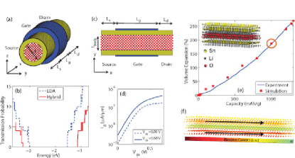
Figure 1: (a) Schematic view of a 3-D gate-all-around nanowire field-effect transistor (GAA NWFET) with a source length $L_{s}$, gate length $L_{g}$, and drain length $L_{d}$, as well as a diameter $d$. Red dots indicate atoms. The semiconducting channel is surrounded by an oxide, represented as a uniform yellow layer. Electron transport occurs along the $x$-axis, while $y$ and $z$ are directions of confinement. (b) Energy-resolved transmission probability through a Si nanowire with $d$=2.2 nm, a length $L$=34.8 nm, and composed of $N_{A}$=10560 atoms. Results obtained with the local density approximation (blue lines) [34] and the HSE06 hybrid functional (red lines) [8] are compared to each other. (c) Same as (a), but for a 2-D double-gate ultra-thin-body field-effect transistor (DG UTBFET) of thickness $t_{body}$. Here, contrary to the nanowire case, the $z$-direction (out-of-plane) is assumed periodic. (d) Transfer characteristics $I_{d}$-$V_{gs}$ of a Si DG UTBFET with $t_{body}$=5 nm, $L_{s}$=$L_{d}$=20 nm, and $L_{g}$=10 nm. (e) Measured [36] and simulated [37] volume expansion of tin-oxide (SnO) in the anode of a lithium-ion battery. The inset shows the atomic structure of a lithiated SnO sample with a capacity $C$=1000 mAh/g. (f) Electronic current through the structure depicted in the inset of (e). The two arrows indicate the current direction. The current flow through the central Li-oxide is insignificant.

The effective mass approximation (EMA), k$\cdot$p models [4], tight-binding [5], or pseudopotential methods [6] offer a satisfactory level of accuracy in many applications, but generally they suffer from several deficiencies such as their necessary parameterization (all are empirical models), the transferability of the parameters from bulk to nanostructures, the treatment of heterostructures, or the absence of atomic resolution for EMA and k$\cdot$p. Ab-initio methods, e.g. density-functional theory (DFT) based on the Kohn-Sham equations [7] appear to be more promising solutions since they address the shortcomings mentioned above and their known band gap underestimations can be corrected with hybrid functionals [8].

First-principles codes such as VASP [9], ABINIT [10], Quantum ESPRESSO [11], SIESTA [12], or CP2K [13] extensively use DFT and therefore lend themselves ideally to the calculation of electronic and crystal structures, phase diagrams, charge densities, or vibrational frequencies in solids. However, they are not well-suited to deal with out-of-equilibrium situations, where, for example, an external voltage or temperature gradient is applied to a nanostructure, inducing an electron current between its contacts. Being able to rapidly and efficiently engineer the magnitude and the direction of this current is a goal of utmost importance in transistor [14], molecular switch [15], quantum well solar cell [16], quantum dot light-emitting diode [17], nanowire thermoelectric generator [18], switching resistive memory [19], or lithium-ion battery [20] research. All these devices rely on optimized current flows that can be directly compared to measurements, contrary to electronic structures, charge distributions, or potential profiles.

To study the transport rather than the static properties of matter, standard DFT packages must be augmented with quantum transport (QT) simulation capabilities, which implies replacing the computation of large eigenvalue problems by the solution of linear systems of equations, as produced by the versatile Non-equilibrium Green’s Function (NEGF) formalism [21]. While ab-initio tools combining DFT and NEGF have been formally demonstrated many years ago [22, 23, 24, 25], they remain computationally very intensive, thus limiting their application to small systems composed of up to 1000 atoms like molecules, nanotubes, or nanoribbons, all simulated in the ballistic limit of transport (no scattering) [26, 27, 28, 29, 30]. There are two notable exceptions where the authors claim to have reached 20000 atoms with a first-principles NEGF scheme [31, 32]. In both studies a linearized muffin-tin-orbital (LMTO) basis is employed, which exhibits a tight-binding-like sparsity pattern that is mostly suitable for close-packed metallic crystals, not for arbitrary materials, as inspected here.

To allow for the simulation of realistic nano-devices made of any elements we propose in this paper a new ab-initio quantum transport solver that goes beyond the existing solutions. The selected approach links two state-of-the-art, massively parallel codes, CP2K [13] and OMEN [33], and leverages their DFT and transport capabilities, respectively, in order to handle systems composed of tens of thousands of atoms. The main target applications are the design of nanoscale transistors and the enhancement of the electronic conductivity in lithium ion battery electrodes, as shown in Fig. 1. These are two research areas with a tremendous need for novel simulation tools. The implementation of the code is general enough to treat other types of nanostructures too.

OMEN already possesses advanced numerical algorithms capable of breaking the petascale barrier while performing quantum transport calculations, but they are optimized for tight-binding bases, not for DFT ones, and they are restricted to CPUs only [33]. Hence, a more powerful sparse linear solver called SplitSolve has recently been developed and integrated into OMEN. It supports the usage of CPUs and GPUs at the same time, significantly reducing the time-to-solution of DFT+QT problems and opening the door for the exploration of larger design spaces. With SplitSolve, the simulation of a Si nanowire transistor composed of 55488 atoms has been successfully achieved, which is, to the best of the authors’ knowledge, at least 10 times larger than what others have reported so far in the literature for similar 3-D semiconducting structures. On the Cray-XK7 Titan at Oak Ridge National Laboratory (ORNL) we have also been able to demonstrate a sustained double-precision performance of 15 PFlop/s in production mode.

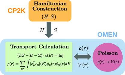
Figure 2: Illustration of the OMEN+CP2K coupling scheme. For a given structure driven out-of-equilibrium, the Hamiltonian $H$ and overlap $S$ matrices produced by CP2K are transferred to OMEN, which uses them to solve electron transport based on the self-consistent solution of the Schrödinger and Poisson equations. More than 99% of the simulation time is spent in OMEN.

The paper is organized as follows: in Section 2, an overview of the ab-initio quantum transport approach is given, followed by the algorithmic innovation in Section 3. A short description of the CP2K and OMEN applications is proposed in Section 4. The time-to-solution, scalability, and peak performance of the code are presented and analyzed in Section 5 before conclusion.

2. SIMULATION APPROACH

A. Density-Functional Theory with a Localized Basis

The coupling between OMEN and CP2K is schematized in Fig. 2. For a given nanostructure, CP2K starts by solving the Kohn-Sham DFT equation [7]

$$\left(-\frac{\hbar^{2}}{2m_{0}}\nabla^{2}+V(r)+V_{H}(r)+V_{xc}(r)\right)\psi(r)=E\psi(r)$$ (1)

where the first term refers to the electron kinetic operator, the second one, $V(r)$, to the electron-nuclei interactions, the third one, $V_{H}(r)$, to the Hartree (Coulomb) potential, and the last one, $V_{xc}(r)$, to the exchange-correlation energy. The wave function $\psi(r)$ is expanded in a localized basis made of contracted Gaussian orbitals

$$\psi(r) = \sum_{\mu}c_{\mu}\phi_{\mu}(r).$$ (2)

In Eq. (2) $\phi_{\mu}(r)$ is a contracted Gaussian function of type $\mu$ and $c_{\mu}$ the corresponding expansion coefficient. Inserting this expression into the Kohn-Sham equation Eq. (1) gives rise to a generalized eigenvalue problem

$$H\cdot c = E\cdot S\cdot c$$ (3)

with the Hamiltonian $H$ and overlap $S$ matrices as well as the unknown expansion coefficients $c$ (now a vector) and eigenvalues $E$. All results presented later in this paper rely on a 3SP basis within the local density approximation (LDA) to model the exchange-correlation energy [34]. However, the SplitSolve algorithm works with any basis set and functional, as shown in Fig. 1: the current flowing through a lithiated SnO battery anode was calculated with a double-$\zeta$ basis and the PBE general gradient approximation (GGA) [35], while the transmission probability through a Si nanowire was obtained with the hybrid HSE06 functional [8].

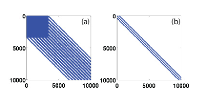
Figure 3: Sub-set of the Hamiltonian matrix corresponding to a UTBFET as shown in Fig. 1(b) with $t_{body}$=5 nm. (a) In the contracted Gaussian basis used in CP2K. (b) In a tight-binding basis. The number of non-zero entries increases by two orders of magnitude in DFT as compared to tight-binding.

B. Quantum Transport

For efficient simulations of transport through nanostructures, it is very convenient to work within a localized basis, as the one provided by CP2K. A sparse matrix, usually block tri-diagonal, then describes the on-site and inter-atomic interactions. The main difference to Eq. (3) is that open boundary conditions (OBCs) must be introduced to inject electrons at the predefined contacts. These so-called reservoirs or leads might experience different chemical potentials, depending on the externally applied bias. This split induces a current flow. The resulting system of equations has the following form in the Non-equilibrium Green’s Function formalism

$$\left(E\cdot S-H-\Sigma^{RB}(E)\right)\cdot G^{R}(E) = \mathbb{1},$$ (4)

where $S$ and $H$ are directly imported from CP2K, the OBCs are cast into the boundary self-energy $\Sigma^{RB}(E)$, $\mathbb{1}$ is the identity matrix, and the unknowns are the retarded Green’s Functions $G^{R}(E)$. In the ballistic limit of transport, as here, it is computationally more efficient to transform Eq. (4) into the Wave Function formalism, which takes the form of a linear system of equations [38]

$$\left(E\cdot S-H-\Sigma^{RB}\right)\cdot c(E) = Inj(E).$$ (5)

The vector $Inj(E)$ denotes the injection mechanism into the out-of-equilibrium devices, whereas $c(E)$ has the same meaning as in Eq. (3). The structure of Eq. (5) is plotted in Fig. 4, highlighting its sparse linear pattern. The charge and current densities can be directly derived from $G^{R}(E)$ or $c(E)$ after Eq. (4) or (5) have been solved for all potential electron energies $E$ and wave vectors $k$ in cases of periodicity along at least one direction [39].

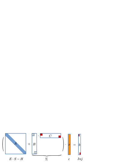
Figure 4: Sparsity pattern of Eq. (5) and its representation as a $Tx=b$ sparse linear system of equations with $T=(E\cdot S-H-\Sigma^{RB})$.

The matrices $H$ and $S$ from CP2K contain about 100 times more non-zero entries than their tight-binding or LMTO counterparts, as shown in Fig. 3. This is why the standard algorithms of OMEN [33] do not perform well in large ab-initio quantum transport calculations. We note that CP2K currently does not provide any momentum- or $k$-dependence for $H$ and $S$ in periodic systems. This issue is resolved by first cutting all the needed blocks from 3-D simulations and then generating $H(k)$ and $S(k)$ in OMEN.

3. ALGORITHMIC INNOVATIONS

A. Open Boundary Conditions: the FEAST Algorithm

The self-energy $\Sigma^{RB}$ and the injection vector $Inj$ in Eq. (5) are calculated from the wave vectors $k_{B}$ and eigenmodes $u_{B}$ of the leads/reservoirs of the considered systems [39]. The following polynomial eigenvalue problem must be solved to obtain them

$$\sum_{l=-N_{\mathrm{BW}}}^{+N_{\mathrm{BW}}}{\textrm{e}^{i\cdot l\cdot k_{B}}(H_{q,q+l}-E\cdot S_{q,q+l})u_{B}}=0,$$ (6)

where $H_{q,q+l}$ and $S_{q,q+l}$ are the parts of the Hamiltonian and overlap matrix that describe the interaction of unit cell $q$ and $q+l$ within the leads and $N_{\mathrm{BW}}$ indicates the range of the inter-cell interactions, typically $N_{\mathrm{BW}}\geq$2. It has been demonstrated that in a tight-binding basis, $\Sigma^{RB}$ can be more rapidly evaluated with Eq. (6) and a shift-and-invert approach [38] than with the standard iterative decimation technique used in NEGF [40]. However, in a DFT basis, the open boundary conditions start to represent a serious computational bottleneck due to the size increase of the involved matrices and the difficulty to parallelize the shift-and-invert method.

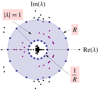
Figure 5: Selected contour in the complex plane to enclose only the $m$ eigenvalues corresponding to propagating and slow decaying modes (red dots). The black dots ($|\lambda|<$1/R and $|\lambda|>$R) are neglected.

In practice it is not necessary to determine the $N_{BC}$ possible phase factors $\lambda=\textrm{e}^{i\cdot k_{B}}$ as the contribution from fast decaying modes is negligible. It suffices to find the $m$ eigenvalues inside an annulus around $|\lambda|=1$ in the complex plane centered at the origin. Hence, a contour integration method can be employed to find a subspace projector $Q_{F}$ that spans the same space as the eigenvectors corresponding to the eigenvalues enclosed by the shaded region in Fig. 5. The FEAST algorithm [41] and its extension to generalized eigenvalue problems with non-Hermitian matrices [42] has been chosen to produce $Q_{F}$. When applying the Rayleigh-Ritz method, the eigenvalue problem reduces to a $m\times m$ system

$$\left[Q_{F}^{\dagger}A_{F}Q_{F}\right]u_{B} = \lambda\left[Q_{F}^{\dagger}B_{F}Q_{F}\right]u_{B}$$ (7)

with the following matrix definitions

$$A_{F} = \left(\begin{array}[]{cccc}\tilde{H}_{-N_{\mathrm{BW}}+1}&\ldots&\tilde{H}_{N_{\mathrm{BW}}-1}&\tilde{H}_{N_{\mathrm{BW}}}\\ \mathbb{1}&&&\\ &\ddots&&\\ &&\mathbb{1}&\\ \end{array}\right),$$ (12)

$$B_{F} = \left(\begin{array}[]{cccc}-\tilde{H}_{-N_{\mathrm{BW}}}&&&\\ &\mathbb{1}&&\\ &&\ddots&\\ &&&\mathbb{1}\end{array}\right),$$ (17)

$$Q_{F} = \sum_{p=1}^{N_{p}}{\frac{z_{p}}{N_{p}}\left(z_{p}B_{F}-A_{F}\right)^{-1}B_{F}\cdot Y_{F}}.$$ (18)

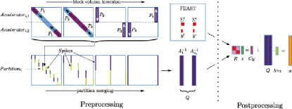
Figure 6: Graphical overview of the SplitSolve algorithm on $p$ accelerators. The system to solve is partitioned into $p$/2 horizontal partitions. Each partition is processed by two accelerators with perfect parallelism. To obtain $Q=[A^{-1}_{1},A^{-1}_{n_{B}}]$, the first and last block columns of $A^{-1}$, the partitions are merged recursively based on the SPIKE algorithm [48]. Upon availability of the boundary conditions $\Sigma^{RB}$ and the injection vectors $b$=$Inj$, the postprocessing phase begins. It mainly consists of solving a small system $R$ and performing a matrix multiplication.

Here, $\tilde{H}_{j}=H_{q,q+j}-E\cdot S_{q,q+j}$, the not-shown entries are equal to 0, the size of $A_{F}$ and $B_{F}$ is $N_{BC}\times N_{BC}$, that of $Q_{F}$ and $Y_{F}$ (matrix of random numbers) $N_{BC}\times m$ with $N_{BC}\gg m$, and the $z_{p}$ are the integration points in the trapezoid rule. The linear systems of equations in Eq. (18) determine the execution time of FEAST. Through an analytical block LU decomposition, their size can be decreased to $N_{BC}/(2N_{\mathrm{BW}})$. Furthermore, they can be solved in parallel since the solution at each of the $N_{p}$ integration points is independent from the others. FEAST can be modified according to Ref. [43] to further reduce the calculation time.

B. Schrödinger Equation: the SplitSolve Algorithm

A parallel direct sparse linear solver such as MUMPS [46] or a custom-made block cyclic reduction (BCR) [33] are typically needed to solve the Schrödinger equation with OBCs. Iterative solvers cannot be efficiently used due to the presence of multiple right-hand-sides. Since our BCR method relies on the sparsity provided by a tight-binding basis, it does not work with DFT, whereas MUMPS becomes slow when the number of non-zero entries in the Hamiltonian and overlap matrices increases drastically. To address these issues we have developed the SplitSolve algorithm that can solve Eq. (5) on accelerators (GPUs or others) and leverage its particular structure displayed in Fig. 4. The matrix $T=(E\cdot S-H-\Sigma^{RB})$ is of size $N_{SS}$ (total number of atoms times orbital per atom) with a block tridiagonal shape. The right-hand-side $Inj$ has multiple columns and non-zero elements only in the top and bottom block rows. Consequently, solving such a system is equivalent to obtaining the first and last block columns of $T^{-1}$ and multiplying them with the non-zero rows of $Inj$.

The goal of SplitSolve is twofold: (i) efficiently computing only the required parts of $T^{-1}$ and (ii) decoupling the calculation of the open boundary conditions $\Sigma^{RB}$ from the solution of $T^{-1}$. This can be achieved by choosing a suitable low rank product representation of the boundary self-energy $\Sigma^{RB}\vcentcolon=BC$, as in Fig. 4, and by recalling the Sherman-Morrison-Woodbury formula

$$(A+BC)^{-1}=A^{-1}-A^{-1}B(\mathbb{1}+CA^{-1}B)^{-1}CA^{-1}.$$

By doing so the computation of $\Sigma^{RB}$ can be interleaved with the solution of the full problem. A similar approach has been successfully tested in Refs. [44, 45] for tight-binding. Defining $x\vcentcolon=c$, $b\vcentcolon=Inj$ and introducing $Q\vcentcolon=A^{-1}B$ and $y\vcentcolon=A^{-1}b$, it follows that

$$x = T^{-1}b\quad=\quad(A-BC)^{-1}b$$ (19)

$$= y+Q(\mathbb{1}-CQ)^{-1}Cy$$ (20)

$$= y+Qz,$$ (21)

where $R\vcentcolon=(\mathbb{1}-CQ)$ and $z\vcentcolon=R^{-1}Cy$. The final solution $x$ is then obtained in four steps

• Step 1 Solve $AQ=B$ for $Q$.

• Step 2 Solve $Ay=b$ for $y$.

• Step 3 Solve $Rz=(\mathbb{1}-CQ)z=Cy$ for $z$.

• Step 4 Compute the full solution as $x=y+Qz$.

The choice of the $B$ and $C$ matrices is free to a large extent, but critical to minimize the computational burden. In SplitSolve $B$ is a $N_{SS}\times 2s$ zero matrix, except the $s\times s$ top left and bottom right subblocks which are equal to $\mathbb{1}$, while $C$ is a $2s\times N_{SS}$ matrix with the top left block set to $\Sigma^{RB,L}$ and the bottom right one to $\Sigma^{RB,R}$, the boundary self-energies of the left ($L$) and right ($R$) contacts, both of size $s\times s$. Given this selection of $B$ and $C$ the following observations are made about SplitSolve:

• The algorithm can be decomposed into a pre- and post-processing phase. The former consists of Step 1 and can be computed in parallel with the evaluation of $C$ and $b$. The latter comprises Steps 2, 3, and 4 and must be performed after the completion of the $Q$, $C$ and $b$ computation.

• The structure of $A$ prior to the addition of the boundary conditions is preserved and can be leveraged in the preprocessing phase: $A$ is usually real symmetric in 3-D structures and complex Hermitian in 1-D and 2-D.

• In terms of numerics, $Q$ consists of the first and last $s$ columns of $A^{-1}$, $y$ can be obtained as $Q\cdot b$, $R$ is a system of comparably small size $2s\times 2s$, and $x$ can be computed as $x=Q\cdot(b^{\prime}+z)$ where $b^{\prime}$ denotes the nonzero rows of $b$.

SplitSolve Preprocessing: To calculate the first and last $s$ columns of $A^{-1}$ in Step 1, a modified version of the recursive Green’s Function (RGF) algorithm [47] has been implemented. If $A_{i,j}$ denotes the $i^{\textrm{th}}$ block row and $j^{\textrm{th}}$ block column of the block tridiagonal matrix $A$ with $n_{B}$ diagonal blocks, then the preprocessing part of SplitSolve can be summarized as in Algorithm 1.

Algorithm 1 Block column inversion on accelerators

  $X_{n_{B}+1}\leftarrow 0$

  $Q_{0}\leftarrow-\mathbb{1}$ {Phases $P_{1}$ & $P_{2}$ in Fig. 6}

  for $i=n_{B}\rightarrow 1$ do

     Solve $(A_{i,i}-A_{i,i+1}\cdot X_{i+1})\cdot X_{i}=A_{i,i-1}$ for $X_{i}$

  end for{Phases $P_{3}$ & $P_{4}$ in Fig. 6}

  for $i=1\rightarrow n_{B}$ do

     $Q_{i}\leftarrow-X_{i}\cdot Q_{i-1}$

  end for

This gives $Q_{i,1:s}$=$A^{-1}_{i,1}$, the first block column of $A^{-1}$. The last one, $Q_{i,s+1:2s}$=$A^{-1}_{i,n_{B}}$, can be derived similarly and in parallel with $A^{-1}_{i,1}$ since the two tasks are independent from each other and naturally scale to two accelerators. Alternatively, the matrix $A$ can be partitioned horizontally into two parts of equal size and the preprocessing in SplitSolve includes four phases, $P_{1}$ to $P_{4}$, as illustrated in Fig. 6.

To study transport through realistic nanostructures it is crucial to parallelize SplitSolve beyond two accelerators so that large system of equations can be efficiently solved. In our implementation, the number of partitions must be a power of 2. Each pair of accelerators computes the first and last block columns of the inverse corresponding to its local partition using Algorithm 1. In a second step adjacent partitions are recursively merged together based on a modified and optimized variant of the SPIKE algorithm [48]. With the proposed scheme the merging steps have a constant cost, their computation is evenly distributed over all the accelerators, and their number grows logarithmically with the number of partitions. The parallelization incurs very little memory overhead so that the extra memory gained by the presence of additional accelerators allows to treat bigger devices.

SplitSolve Postprocessing: Upon availability of $Q$, $\Sigma^{RB}$, and $b$, the matrices $R$ and $Cy$ are constructed on the two accelerators storing the first and last partition and calculating $z$. This quantity is then distributed to all the accelerators to solve Eq. (21) with one single matrix-vector multiplication per block, i.e. $x=Q\cdot(b^{\prime}+z)$.

C. Node-Level FEAST and SplitSolve Performance

The performance of the newly implemented FEAST+SplitSolve approach has been tested on the Cray-XC30 Piz Daint at the Swiss National Supercomputing Centre (CSCS) [49] and on the Cray-XK7 Titan at Oak Ridge National Laboratory (ORNL) [50]. More details about both machines are given in Section 5A. Relevant is that they both offer hybrid nodes with CPUs and GPUs. The main features of FEAST+SplitSolve are then the following:

• The calculation of the OBCs and the solution of Eq. (5) are interleaved, FEAST being executed on the CPUs, while SplitSolve employs the GPUs;

• All the operations in FEAST, e.g. the solution of Eq. (6) rely on BLAS [51] and LAPACK [52], mostly zgemm, zggev, and zgesv;

• In SplitSolve, the matrix $A=(E\cdot S-H)$ is distributed over all the available GPUs and stored in their memory. Half of the matrix $Q$ is stored on the GPUs and half on the CPUs to reduce the memory consumption. The induced CPU$\leftrightarrow$GPU data transfer overlaps with computation (no cost);

• The calculation of each $Q_{i}$ block in Alg. 1 requires two matrix-matrix multiplications, one LU factorization, and one backward substitution. All the involved matrices are either dense or treated as such to leverage the cuBLAS (d/zgemm) [53] and MAGMA (zgesv_nopiv_gpu) [54] libraries.

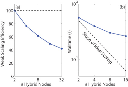
Figure 7: Scaling performance of the SplitSolve algorithm on the Cray-XC30 Piz Daint. A Si UTBFET with $t_{body}=5$ nm is used as test bed. (a) Weak scaling efficiency with a constant number of atoms per GPU (2560, $N_{SS}=N_{GPU}\times 30720$). The efficiency drops as the GPU count increases because of the additional spike calculations, as shown in Fig. 6. (b) Strong scaling for a device containing 10240 atoms ($t_{body}=5$ nm, $L=34.8$ nm, $N_{SS}=122880$). The poor scalability is due to the structure size, which is the largest that 2 GPUs can handle, but does not offer enough workload for $\geq$8 GPUs.

The weak and strong scaling of FEAST+SplitSolve on Piz Daint are reported in Fig. 7 for a 2-D ultra-thin-body field-effect transistor (UTBFET), as in Fig. 1(c). All CPUs and GPUs per hybrid node are used. The calculation of the OBCs with FEAST is completely hidden by the solution of Eq. (5). The relatively low weak scaling efficiency originates from the extra calculation of spikes, which are required to parallelize the workload beyond 2 GPUs. These spikes are depicted in Fig. 6. Their generation takes 10 sec per recursive step so that the total simulation time increases from 30 sec on 2 GPUs (1 partition) up to 70 sec on 32 GPUs (16 partitions, 4 recursive steps). In the strong scaling case, the limitation comes from the impossibility to have a device structure that is large enough to create enough work on 16 GPUs and small enough to fit onto 2 GPUs.

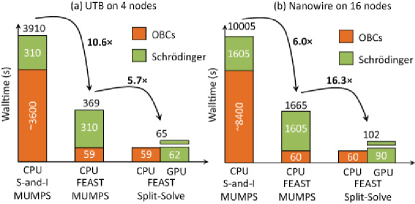
Figure 8: Comparison of three different algorithms to solve the Schrödinger equation with OBCs on Titan at one given electron momentum and energy for (a) a Si UTBFET with $t_{body}$=5 nm, $L$=78.2 nm, and 23040 atoms (size of $H$/$S$: $N_{SS}$=276480) and (b) a Si NWFET with $d$=3.2 nm, $L$=104.3 nm, and 55488 atoms (size of $H$/$S$: $N_{SS}$=665856). The orange blocks refer to the time for the OBC calculation, the green ones to the time for the solution of Eq. (5). The first algorithm combines a shift-and-invert method for the OBCs [38] with MUMPS [46], in the second one, shift-and-invert is replaced by FEAST [41], while in the third one, SplitSolve is introduced. The speed-up factors between each approach are also reported.

Our strategy is to choose the minimum number of GPUs that can accommodate the desired nanostructure. This is what has been done in Fig. 8 on Titan where the time-to-solution of FEAST+SplitSolve is compared to FEAST+MUMPS [46] and shift-and-invert+MUMPS [38] for a 3-D Si nanowire field-effect transistor (NWFET) composed of 55488 atoms (16 GPUs) and a Si UTBFET with 23040 atoms (4 GPUs). MUMPS_5.0 has been selected because it is faster than SuperLU_dist [55] for these examples. The speedup between shift-and-invert+MUMPS and FEAST+SplitSolve is larger than 50 in both cases, i.e. our algorithms optimized for ab-initio transport calculations significantly outperform those designed for tight-binding problems. Also, SplitSolve alone is between 6 and 16 times faster than MUMPS on the same number of hybrid nodes. These speedups demonstrate that the scaling in Fig. 7 is not a limiting factor.

4. APPLICATION DESCRIPTION

The work flow of the OMEN+CP2K DFT-based quantum transport simulator is summarized in Fig. 2. It is basically a Schrödinger-Poisson solver with open boundary conditions to account for electron flows between contacts. CP2K, which is a freely available DFT package [56], is used here to construct the structure of the investigated nano-devices, relax their atom positions, and generate the corresponding Hamiltonian and overlap matrices. The latter are then transferred to OMEN, which performs quantum transport calculations based on them. This part consumes 99% of the total simulation time and is the focus of this work.

OMEN is a massively parallel, one-, two-, and three-dimensional quantum transport simulator that self-consistently solves the Schrödinger and Poisson equations in nanostructures. The tool was originally based on different flavors of the nearest-neighbor tight-binding model, but it has been extended towards ab-initio capabilities through its link with CP2K and the incorporation of the FEAST+SplitSolve approach presented here. It is important to realize that the OMEN version that produced all the results discussed in the next Section is the same as the one that is used to simulate nano-devices on a daily basis, either in the ballistic limit of transport or in the presence of scattering [57]. OMEN is a real production code and not a software that was only tuned to reach the highest possible performance on a specific instance of a general problem.

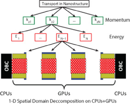
Figure 9: OMEN multi-level distribution of the workload. The electron momentum $k$ and energy $E$ are almost embarrassingly parallel and form the two highest levels. A 1-D spatial domain decomposition is applied to the solution of the Schrödinger equation with open boundary conditions, simultaneously stressing multiple CPUs and GPUs. This is the third level of parallelization.

Although four natural levels of parallelism are available in OMEN, only three have been utilized in this paper, as shown in Fig. 9: the momentum $k$ and energy $E$ points are almost embarrassingly parallel, while FEAST+SplitSolve provides a 1-D spatial domain decomposition. The distribution of the workload is controlled with MPI [58] and a hierarchical organization of communicators. To avoid any work imbalance between sub-communicators corresponding to different $k$ points, a dynamical allocation of the number of nodes per momentum has been developed and verified before [45].

On the implementation side, OMEN is written in C++ and CP2K in Fortran 2003. The coupling between the two packages currently occurs through a transfer of binary files. Not all the nodes running OMEN load the Hamiltonian and overlap matrices, but only those necessary to gather all the unique parts of $H$ and $S$. The resulting data are then distributed to all the available MPI ranks with MPI_Bcast and copied to the GPUs. The parts of CP2K and OMEN ported to GPUs are implemented in the CUDA language from NVIDIA.

	Piz Daint [49]	Titan [50]
Hybrid nodes	5272	18688
GPUs	5272	18688
GPU model	Tesla K20X	Tesla K20X
Cores	42176	299008
CPU model	Intel Xeon E5-2670	Opteron 6274
Node perf. (GFlop/s)	166.4+1311	134.4+1311

TABLE I: Technical specifications of Piz Daint and Titan.

5. PERFORMANCE RESULTS

A. System Description

All the OMEN+CP2K simulations have been run on the Cray-XC30 Piz Daint at CSCS and Cray-XK7 Titan at ORNL. The technical specifications of both machines are summarized in Table I. The codes are compiled with GNU 4.8.2 and CUDA 5.5/6.5 and use the Cray MPICH 7.0.4, libsci 4.9, and MAGMA 1.6.2 libraries with customizations. On Piz Daint, all the CPUs per node are active, while at least half of them remain idle on Titan. The MAGMA function zgesv_nopiv_gpu is responsible for that: it performs a hybrid LU factorization on a CPU core and a GPU. On Titan it has been observed that the factorization time deteriorates if all the CPUs work because the competition between them negatively affects the execution of zgesv_nopiv_gpu. In spite of that SplitSolve is still about 10% slower per node on Titan than on Piz Daint.

B. Measurement Methodology

As can be seen in Algorithm 1 the number of floating point operations (FLOPs) involved in SplitSolve is deterministic and can be accurately estimated. Still, we decided to employ PAPI [59] to measure the CPU FLOPs and the CUPTI library [60] for the GPUs. In the CPU case, the function PAPI_start_counters with Events=PAPI_DP_OPS is placed right after the loading of the Hamiltonian and overlap matrices imported from CP2K, i.e. the input reading time is not accounted for in the performance measurement. Our limited access to the computational resources of Titan is the reason for this neglection: in a full-scale run, loading $H$ and $S$ and setting up the simulation environment takes about 4 minutes. Then each self-consistent Schrödinger-Poisson iteration lasts between 15 and 20 minutes. Knowing that an entire simulation involves roughly 40-50 iterations for 10 bias points, the 4 initial minutes turn negligible. However, due to our limited allocation, we could only simulate 1 or 2 iterations so that accounting for the initialization phase is not representative of the actual code performance. The function PAPI_stop_counters is set at the end of the simulation and includes the output writing time (a couple of seconds).

On the GPUs the FLOPs are obtained by sampling the device counters every second with the function cuptiEventGroupReadEvent. The accuracy of the method has been verified with examples where the number of FLOPs is known, e.g. matrix-matrix multiplications. This approach cannot be used “on-the-fly” since it considerably slows down the execution time. Hence, what is measured is the number of FLOPs that arise from the solution of the OBCs on CPUs and of Eq. (5) on GPUs for one single representative energy point. To find the total FLOPs this result is then multiplied by the total number of energy points that have been calculated.

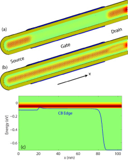
Figure 10: Electron distribution (a), current map (b), and spectral current (c) in a Si GAA NWFET as in Fig. 1(a) with a diameter $d$=3.2 nm, $L_{s}$=$L_{c}$=20 nm, $L_{g}$=64.3 nm, $V_{ds}$=0.6 V, and composed of 55488 atoms. The nanowire transport axis is $x$, which is aligned with the $<$100$>$ crystal axis. In all the sub-plots, red means high concentrations (charge or current) and green none. In (b) and (c) an electron current $I_{d}$=1.5 $\mu$A flows through the nanowire. In (c), the blue line indicates the conduction band edge of the transistor.

C. Time-to-Solution

As explained earlier, ab-initio quantum transport simulations are usually limited to 1000 atoms due to their heavy computational burden. The FEAST+SplitSolve combination makes possible the investigation of much larger nanostructures such as a Si gate-all-around nanowire transistor with a diameter $d$=3.2 nm, a source and drain extension $L_{s}$=$L_{d}$=20 nm, a gate length $L_{g}$=64.3 nm, and a total of 55488 atoms. A schematic view of this device is given in Fig. 1(a), while its atomically resolved charge and current distributions as well as its spectral current are shown in Fig. 10 for one bias point. The structure dimensions are at least one order of magnitude larger than what is reported in the literature and comparable to what is fabricated in laboratories [61]. As indicated in Fig. 8 the computational time per energy point for this nanowire reduces to 102 sec with FEAST+SplitSolve using 16 hybrid nodes of Titan. Hence, it has been measured that a self-consistent Schrödinger-Poisson iteration including 2000 energy points takes less than 10 minutes on 8192 nodes. Knowing that the time per energy point with FEAST+MUMPS is in the order of 30 minutes on 16 nodes, a CPU machine with four times as many nodes would still be 3$\times$ slower than our refined approach.

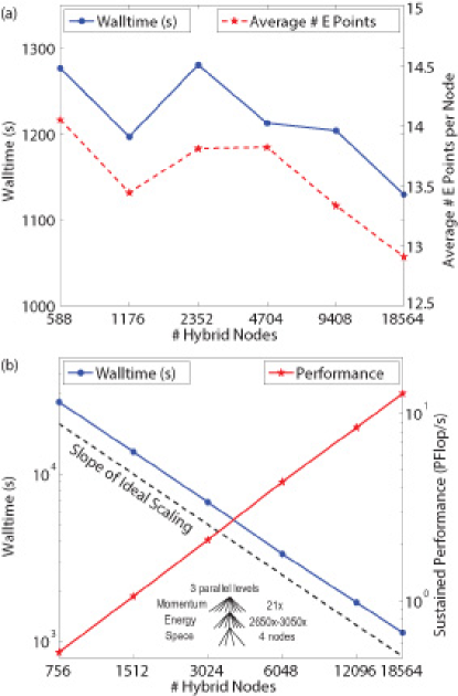
Figure 11: OMEN scaling performance on Titan for a Si DG UTBFET as in Fig. 1(c) with $t_{body}$=5 nm, $L_{s}$=$L_{c}$=20 nm, $L_{g}$=38.2 nm, $V_{ds}$=0.6 V, and $N_{A}$=23040 atoms. In all the simulations, one Schrödinger-Poisson iteration is considered, the total number of $k$-points is equal to 21, the 1-D spatial domain decomposition is performed on 4 hybrid nodes, and three levels of parallelization are used. (a) Weak scaling. The total number of energy points varies so that each node deals with 13 to 14 of them, regardless of the number of used nodes. Note that slight variations are unavoidable, as indicated by the dashed red curve, because the energy grid is not an input parameter, but automatically generated by OMEN based on the minimum and maximum allowed distance between two consecutive energy points. (b) Strong scaling and sustained performance. The number of energy points per momentum varies from 2650 up to 3050.

D. Scalability

The weak and strong scalability of OMEN on Titan, after importing the required Hamiltonian and overlap matrices from CP2K, are presented in Fig. 11 and the data summarized in Tables II and III. A Si double-gate ultra-thin-body transistor, as in Fig. 1(c), with a body thickness $t_{body}$=5 nm, $L_{s}$=$L_{d}$=20 nm, $L_{g}$=38.2 nm, and a total of 23040 atoms has been chosen as test structure of realistic dimensions [62]. In each run, OMEN computed one Schrödinger-Poisson iteration for one single bias point with 21 $k$-points and FEAST+SplitSolve on 4 hybrid nodes. Increasing the number of bias points or self-consistent iterations does not change the scalability of the code since each point/iteration is processed sequentially, one after the other, and the workload is dynamically redistributed after each step [45].

In the weak scaling experiment the average number of energy points that each node deals with should ideally remain constant, but it varies here between 12.9 and 14.1, as detailed in Table II. These differences stem from the fact that the number of calculated energy points is not a direct input parameter, but depends on others, as explained in the caption of Fig. 11. If the extracted simulation times are normalized with the average number of energy point per node, as in the fourth column of Table II, it can be seen that the weak scaling efficiency is good with $\sim$5% variation across all the nodes.

Figure 11(b) shows the strong scaling results of OMEN. The total number of energy points is the same in all the runs (59908), but it varies with the momentum, i.e. $E$ depends on $k$. The simulation time decreases almost linearly when scaling from 756 up to 18564 nodes, reaching a parallel efficiency of 97%. This is not a surprise since the loop over the momentum and energy points is embarrassingly parallel, but it demonstrates that the code performs as expected.

E. Peak Performance

OMEN running FEAST+SplitSolve for the same UTB transistor as before initially reached a sustained performance of 12.8 PFlop/s in double-precision, as indicated in Table III. The solution of the OBCs and Eq. (5) for each of the 59908 computed energy points consumes 241 TFLOPs, 11 for the OBCs on the CPUs (5%) and 230 for SplitSolve on the GPUs (95%). The bottleneck is the LU factorization and backward substitution in Alg. 1. They are done with the MAGMA function zgesv_nopiv_gpu that does not perform as well on Titan as on Piz Daint. Replacing zgesv_nopiv_gpu with zhesv_nopiv_gpu and profiting from the property that the matrix $A=(E\cdot S-H)$ is Hermitian in 2-D structures (UTBFET) helps decrease SplitSolve’s execution time per energy point [63]. By combining this trick with further profiling and tuning of the code as well as algorithm adaptations to Titan, the double-precision sustained performance increased to 15.01 PFlop/s in production mode. Exactly the same structure as the one producing 12.8 PFlop/s was used for that purpose, but the simulation time decreased from 1130 down to 912.5 sec, while the number of operations per energy point went down from 241 to 228 TFLOPS.

Hybrid Nodes	Time (s)	Avg. $E$/node	Avg. Time/$E$ (s)
588	1277	14.1	90.8
1176	1197	13.4	89
2352	1281	13.8	92.7
4704	1213	13.8	87.7
9408	1204	13.3	90.3
18564	1130	12.9	87.5

TABLE II: Weak scaling data corresponding to Fig. 11(a).

Hybrid Nodes	Time (s)	$||$ Eff. (%)	PFlop/s
756	26975	100	0.54
1512	13593	99.2	1.06
3024	6806	99.1	2.12
6048	3415	98.7	4.23
12096	1711	98.5	8.45
18564	1130	97.3	12.8
18564	912.5	-	15.01

TABLE III: Strong scaling data corresponding to Fig. 11(b) and to the run that reached 15 PFlop/s (last line).

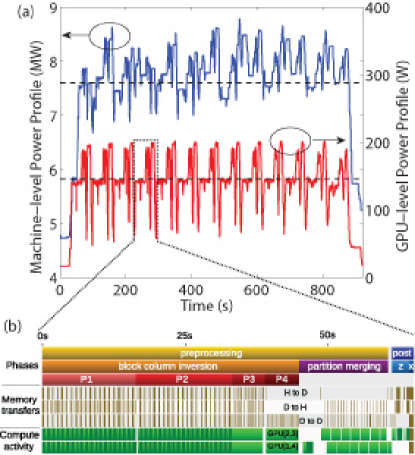
Figure 12: (a) Machine-level (left $y$-axis, blue line) and GPU-level (right $y$-axis, red line) power profile extracted from the run that reached a sustained performance of 15 PFlop/s. On average, Titan consumed 7.6 MW during this UTB simulation (1975 MFLOPS/W), whereas each GPU utilized 146 W (5396 MFLOPS/W). The machine-level power profile includes the hardware usage (CPU+GPU), the pumping power used by the XDPs, the fan energy from the blower in each cabinet, as well as the line loss from the switchboards to the cabinets. (b) Typical GPU activity measured with nvprof during the calculation of one energy point (4 GPUs with indices 1 to 4 are involved). The SplitSolve phases from Fig. 6 are indicated together with the host-to-device (H-to-D), device-to-host (D-to-H), and device-to-device (D-to-D) memory transfers as well as the compute activity.

The machine- and GPU-level power profiles of the simulation that reached 15 PFlop/s are plotted in Fig. 12(a). The 13 energy points that each group of 4 GPUs treats can be identified at both levels, but the GPU-level matches better with the different algorithm phases. The peak power consumption of Titan during this run is equal to 8.8 MW, its average to 7.6 MW, which corresponds to 1975 MFLOPS/W. At the GPU level, the computational efficiency increases to 5396 MFLOPS/W. Finally, in Fig. 12(b), the typical GPU utilization (measured with nvprof) is reported for the calculation of one energy point. Note the high utilization and well-overlapped computation-communication pattern.

6. CONCLUSION

By linking two existing applications, CP2K and OMEN, developing SplitSolve, an innovative, GPU-based, algorithm, and combining it with a parallel eigenvalue solver, FEAST, we have been able to redefine the limit of ab-initio quantum transport simulations. Significant improvements have been achieved in terms of structure dimensions (10$\times$ larger), sustained performance (15 PFlop/s), and time-to-solution ($>$50$\times$ shorter). While standard approaches are typically limited to 1000 atoms, we have reached more than 50000 for a 3-D nanowire structure and 23040 for a 2-D ultra-thin-body.

SplitSolve heavily relies on the structure of the matrices encountered in quantum transport calculations (block tri-diagonal + sparse right-hand-side) to deliver its best efficiency, but these properties can be found in other research fields such as computational fluid dynamics or in the solution of the Poisson equation. Hence, our multi-GPU sparse linear solver is not limited to one single problem, rather it may be applied to others.

From 2011 to 2015 the sustained performance of OMEN increased by one order of magnitude, going from 1.28 PFlop/s on the former Cray-XT5 Jaguar up to 15 PFlop/s on Titan, mainly through algorithmic and hardware improvements. A roofline analysis of SplitSolve and FEAST shows that both algorithms have high arithmetic intensity and are clearly compute bound. It can thus be expected that OMEN will run efficiently on future supercomputing systems offering lower relative memory bandwidth, but higher computational power such as the next-generation CORAL machines.

References

- [1] M. Fuechsle et al., “A single-atom transistor”, Nature Nano. 7, 242 (2012).
- [2] J. Cai et al., “Atomically precise bottom-up fabrication of graphene nanoribbons”, Nature 466, 470-473 (2010).
- [3] C.-H. Lee et al., “Atomically thin p–n junctions with van der Waals heterointerfaces”, Nature Nano. 9, 676 (2014).
- [4] J. M. Luttinger and W. Kohn, “Motion of Electrons and Holes in Perturbed Periodic Fields”, Physical Review 97, 869 (1955)
- [5] J. C. Slater and G. F. Koster, “Simplified LCAO Method for the Periodic Potential Problem”, Phys. Rev. 94, 1498-1524 (1954).
- [6] J. C. Philips, “Energy-Band Interpolation Scheme Based on a Pseudopotential”, Phys. Rev. 112, 685 (1958).
- [7] W. Kohn and L. J. Sham, “Self-Consistent Equations Including Exchange and Correlation Effects”, Phys. Rev. 140, A1133 (1965).
- [8] J. Heyd and G. E. Scuseria, “Assessment and validation of a screened Coulomb hybrid density functional”, J. Chem. Phys. 120, 7274-7280 (2004).
- [9] G. Kresse and J. Furthmüller, “Efficient iterative schemes for ab initio total-energy calculations using a plane-wave basis set” , Phys. Rev. B 54, 11169 (1996).
- [10] X. Gonze et al., “ABINIT : First-principles approach of materials and nanosystem properties”, Comp. Phys. Comm. 180, 2582 (2009).
- [11] P. Giannozzi et al.,“QUANTUM ESPRESSO: a modular and open-source software project for quantum simulations of materials”, J. of Physics: Condensed Matter, 39, 395502 (2009).
- [12] J. Izquierdo et al..“Systematic ab initio study of the electronic and magnetic properties of different pure and mixed iron systems”, Phys. Rev. B 61, 13639 (2000).
- [13] J. VandeVondele, M. Krack, F. Mohamed, M. Parrinello, T. Chassaing, and J. Hutter, “Quickstep: fast and accurate density functional calculations using a mixed Gaussian and plane waves approach”, Comp. Phys. Comm. 167, 103 (2005).
- [14] B. S. Doyle et al., “High Performance Fully-Depleted Tri-Gate CMOS Transistors”, IEEE Elec. Dev. Lett. 24, 263 (2003).
- [15] C. Joachim et al., “Electronics using hybrid-molecular and mono-molecular devices”, Nature 408, 541 (2000).
- [16] K. Barnham and G. Duggan, “A new approach to high-efficiency multi-band-gap solar cells”, J. App. Phys. 67, 3490 (1990).
- [17] P. O. Anikeeva et al., “Quantum Dot Light-Emitting Devices with Electroluminescence Tunable over the Entire Visible Spectrum”, Nano Letters 9, 2532 (2009).
- [18] A. I. Hochbaum et al., “Enhanced thermoelectric efficiency of rough silicon nanowires”, Nature 451, 163 (2008).
- [19] R. Waser and M. Aono, “Nanoionics-based resistive switching memories”, Nature Materials 6, 833 (2007).
- [20] S.-Y. Chung, J. T. Bloking, and Y.-M. Chiang, “Electronically conductive phospho-olivines as lithium storage electrodes”, Nature Materials 1, 123 (2002).
- [21] S. Datta, “Electronic Transport in Mesoscopic Systems”, Cambridge University Press (1995).
- [22] J. Taylor, H. Guo, and J. Wang, “Ab initio modeling of quantum transport properties of molecular electronic devices”, Phys. Rev. B 63, 245407 (2001).
- [23] M. Brandbyge, J. L Mozos, and P. Ordejon, J. Taylor, and K. Stokbro, “Density-functional method for nonequilibrium electron transport”, Phys. Rev. B 74, 165401 (2002).
- [24] K. Stokbro, J. Taylor, M. Brandbyge, and P. Ordejon, “TranSIESTA: a spice for molecular electronics”, Nanotech. 2, 82 (2003).
- [25] Y. Xue, S. Datta and M. A. Ratner, “First-principles based matrix Green’s function approach to molecular electronic devices: general formalism”, Chemical Physics 281, 151 (2002).
- [26] D. Sharma et al., “Transport properties and electrical device characteristics with the TiMeS computational platform: Application in silicon nanowires”, J. Appl. Phys. 113, 203708 (2013).
- [27] Q.-H. Wu, P. Zhao, and D.-S. Liu, “First-Principles Study of the Rectifying Properties of the Alkali-Metal-Atom-Doped BDC60 Molecule”, Acta Physico-Chimica Sinica 30, 53 (2014).
- [28] Y. Matsuura, “Tunnel current across linear homocatenated germanium chains”, J. App. Phys. 115, 043701 (2014).
- [29] B. Magyari-Kope, L. Zhao, K. Kamiya, M. Y. Yang, M. Niwa, K. Shiraishi, and Y. Nishi, “The Interplay between Electronic and Ionic Transport in the Resistive Switching Process of Random Access Memory Devices”, ECS Transactions 64 153-158 (2014).
- [30] A. Fediai, D. A. Ryndyk, and G. Cuniberti, “Electron transport in extended carbon-nanotube/metal contacts: Ab initio based Green function method”, Phys. Rev. B 91, 165404 (2015).
- [31] K. Xia, M. Zwierzycki, M. Talanana, and P. J. Kelly, G. E. W. Bauer, “First-principles scattering matrices for spin transport”, Phys. Rev. B 73, 064420 (2006).
- [32] J. Maassen, M. Harb, V. Michaud-Rioux, Y. Zhu, H. Guo, “Quantum Transport Modeling From First Principles”, Proc. IEEE 101, 518 (2013).
- [33] M. Luisier, T. B. Boykin, G. Klimeck, and W. Fichtner, “Atomistic nanoelectronic device engineering with sustained performances up to 1.44 PFlop/s”, Proceedings of the 2011 International Conference for High Performance Computing, Networking, Storage and Analysis, 2:1–2:11 (2011).
- [34] S. Goedecker, M. Teter, and J. Hutter, “Separable dual-space Gaussian pseudopotentials”, Phys. Rev. B 54, 1703-1710 (1996).
- [35] J. P. Perdew, K. Burke, and M. Ernzerhof, “Generalized gradient approximation made simple”, Phys. Rev. Lett. 77 3865 (1996).
- [36] M. Ebner, F. Marone, M. Stampanoni, and V. Wood, “Visualization and quantification of electrochemical and mechanical degradation in Li ion batteries”, Science 342, 716 (2013).
- [37] A. Pedersen and M. Luisier, “Lithiation of Tin Oxide: A Computational Study”, ACS Applied Materials & Interfaces 6, 22257 (2014).
- [38] M. Luisier, G. Klimeck, A. Schenk, and W. Fichtner, “Atomistic Simulation of Nanowires in the Tight-Binding Formalism: from Boundary Conditions to Strain Calculations, Phys. Rev. B, 74, 205323 (2006).
- [39] M. Luisier and A. Schenk, “Atomistic Simulation of Nanowire Transistors”, J. Comput. Theor. Nanosci. 5, 1031 (2008).
- [40] M. P. L. Sancho, J. M. L. Sancho, and J. Rubio, “Highly Convergent Schemes for the Calculation of Bulk and Surface Green Functions”, J. Phys. F: Met. Phys. 15, 851 (1985).
- [41] E. Polizzi, “Density-matrix-based algorithm for solving eigenvalue problems”, Phys. Rev. B 79, 115112 (2009).
- [42] S. E. Laux, “Solving complex band structure problems with the FEAST eigenvalue algorithm”, Phys. Rev. B 86, 075103 (2012).
- [43] W.-J. Beyn, “An integral method for solving nonlinear eigenvalue problems”, Lin. Alg. Appl. 436, 3839 (2012).
- [44] S. Cauley et al., “A Two-Dimensional Domain Decomposition Technique for the Simulation of Quantum-Scale Devices”, J. Comp. Phy. 231, 1293 (2011).
- [45] M. Luisier and G. Klimeck, “Numerical strategies towards peta-scale simulations of nanoelectronics devices”, Parallel Computing 36, 117-128 (2010).
- [46] P. R. Amestoy, I. S. Duff, and J.-Y. L’Excellent, “Multifrontal parallel distributed symmetric and unsymmetric solvers” Comput. Methods in Appl. Mech. Eng. 184, 501 (2000).
- [47] A. Svizhenko, M. P. Anantram, T. R. Govindan, B. Biegel, and R. Venugopal, “Two-dimensional quantum mechanical modeling of nanotransistors”, J. Appl. Phys. 91, 2343-2354 (2002).
- [48] E. Polizzi and A. Sameh, “A parallel hybrid banded system solver: the SPIKE algorithm”, Par. Comp. 32, 177 (2006).
- [49] http://www.cscs.ch/computers/piz_daint_piz_dora/index.html
- [50] https://www.olcf.ornl.gov/titan/
- [51] J. Dongarra, “Basic Linear Algebra Subprograms Technical Forum Standard”, International Journal of High Performance Applications and Supercomputing, 16, 1–111 (2002).
- [52] E. Anderson, Z. Bai, C. Bischof, S. Blackford, J. Demmel, J. Dongarra, J. Du Croz, A. Greenbaum, S. Hammarling, A. McKenney, and D. Sorensen, “LAPACK User’s Guide”, Third Edition, SIAM, Philadelphia (1999).
- [53] https://developer.nvidia.com/cuBLAS
- [54] http://icl.cs.utk.edu/magma/
- [55] X. S. Li and J. W. Demmel “SuperLU_DIST: A Scalable Distributed Memory Sparse Direct Solver for Unsymmetric Linear Systems”, ACM Trans. on Math. Software 29, 110 (2003).
- [56] http://www.cp2k.org/
- [57] M. Luisier and G. Klimeck, “Atomistic full-band simulations of silicon nanowire transistors: Effects of electron-phonon scattering”, Phys. Rev. B 80, 155430 (2009).
- [58] W. Gropp, E. Lusk, N. Doss, and A. Skjellum, “A high-performance, portable implementation of the MPI message passing interface standard”, Parallel Computing 22, 789 (1996).
- [59] http://icl.cs.utk.edu/papi
- [60] http://docs.nvidia.com/cuda/cupti/index.html
- [61] S. D. Suk et al., “Investigation of nanowire size dependency on TSNWFET”, IEDM Tech. Dig. 2007, 891-894 (2007).
- [62] B. Doris et al., “Extreme scaling with ultra-thin Si channel MOSFETs”, IEDM Tech. Dig. 2002, 267-270 (2002).
- [63] M. Baboulin, J. Dongarra, A. Remy, S. Tomov, and I. Yamazaki, “Dense Symmetric Indefinite Factorization on GPU accelerated architectures”, in the proceedings of International Conference on Parallel Processing and Applied Mathematics (PPAM) (2015).