Experimental Study of the Bottleneck in Fully Developed Turbulence

Abstract

The energy spectrum of incompressible turbulence is known to reveal a pileup of energy at those high wavenumbers where viscous dissipation begins to act. It is called the bottleneck effect donzis_bottleneck_2010 ; falkovich_bottleneck_1994 ; frisch_hyperviscosity_2008 ; kurien_cascade_2004 ; verma_energy_2007 . Based on direct numerical simulations of the incompressible Navier-Stokes equations, results from Donzis & Sreenivasan donzis_bottleneck_2010 pointed to a decrease of the strength of the bottleneck with increasing intensity of the turbulence, measured by the Taylor micro-scale Reynolds number $R_{\lambda}$. Here we report first experimental results on the dependence of the amplitude of the bottleneck as a function of $R_{\lambda}$ in a wind-tunnel flow. We used an active grid griffin_control_2018 in the Variable Density Turbulence Tunnel (VDTT) bodenschatz_variable_2014 to reach $R_{\lambda}>5000$, which is unmatched in laboratory flows of decaying turbulence. The VDTT with the active grid permitted us to measure energy spectra from flows of different $R_{\lambda}$, with the small-scale features appearing always at the same frequencies. We relate those spectra recorded to a common reference spectrum, largely eliminating systematic errors which plague hotwire measurements at high frequencies. The data are consistent with a power law for the decrease of the bottleneck strength for the finite range of $R_{\lambda}$ in the experiment.

I Introduction

Turbulence is omnipresent in natural and technological flows. Its consequences for the associated processes are essential in the fields of astrophysics, geophysics, meteorology, biology, and in many engineering disciplines from chemical engineering, combustion science, heat and mass transfer engineering to aeronautics, marine science and renewable energy research. From the fundamental perspective the mathematical field theory of the incompressible Navier Stokes equation continues to challenges pure and applied mathematicians fefferman_existence_2006 . In turbulence fluid velocities and accelerations fluctuate greatly and any description can only be statistical in nature. It is believed that at very high turbulence levels at spatial scales smaller than the energy injection scale the turbulence shows universal properties, independent of the particular driving. According to Kolmogorov’s phenomenology from 1941 kolmogorov_local_1941 (abbreviated K41), the universal statistical spatial properties of fully developed turbulence can be captured in three ranges of spatial scales. Kinetic Energy is injected into the turbulent fluctuations at the largest scales, whose properties are particular to the driving mechanism. The kinetic energy is transformed into heat at the very smallest scales through viscous dissipation. If the range of spatial scales found in the turbulent structures is large enough, a third range of scales develops, where neither the pecularities of energy injection, nor viscous dissipation influence the spatial scale-to scale energy transfer. This range is called the inertial range. In this intermediate range statistical properties can be interpreted by the scale-to-scale transfer of kinetic energy only, described by the kinetic energy dissipation range $\varepsilon$(dissipated power per unit mass). The dimensionless quantity used to give the strength of turbulence and thus the size of the inertial range scaling is the Taylor microscale Reynolds number

$$R_{\lambda}=\frac{u\lambda}{\nu}.$$

$u$ is the rms of the velocity fluctuations, $\nu$ is the kinematic viscosity of the fluid, and $\lambda$ is the Taylor microscale, which can be thought of as the smallest length scale at which molecular viscosity can be neglected taylor_statistical_1935 . It can therefore be interpreted as a typical size of an inertial range eddy. In statistically isotropic and homogeneous turbulence $R_{\lambda}$ can be linked to the well-known Reynolds number $\text{Re}=uL/\nu$ based on the large scales $L$ via $R_{\lambda}=\sqrt{15\text{Re}}$ taylor_spectrum_1938 . The integral scale $L$ can be estimated as the integral over the velocity correlation function $L_{11}=\int\langle u(x+r)u(r)\rangle dr$.

In K41 phenomenology for spatially homogeneous and statistically isotropic turbulence the spatial energy spectrum in the inertial range is given by

$$E(k)=C_{K}\varepsilon^{2/3}k^{-5/3}.$$ (1)

$C_{K}$ is the Kolmogorov constant, $k$ is the wavenumber. In this K41 spectrum the only free parameter is the dissipation rate $\varepsilon$ as indicated above.

Despite its simplicity, Eq. (1) describes the energy spectrum of observed and simulated turbulent flows quite well (see saddoughi_local_1994 for a compilation). Nevertheless, important deviations are well known. When analyzing the compensated spectrum, $E(k)\varepsilon^{-2/3}k^{5/3}$, deviations from a $k^{-5/3}$ scaling are found. Prominent is an increase in amplitude of the compensated spectrum at the high-wavenumber end of the inertial range. This pileup of energy is commonly called the bottleneck effect verma_local_2005 ; frisch_hyperviscosity_2008 ; kurien_cascade_2004 ; falkovich_bottleneck_1994 ; verma_energy_2007 ; yakhot_hidden_1993 . It has been observed in laboratory flows (e.g. she_universal_1993 ; saddoughi_local_1994 ; kang_decaying_2003; bodenschatz_variable_2014 ) and direct numerical simulations (DNS) khurshid_energy_2018 ; ishihara_energy_2016 ; ishihara_energy_2005 ; donzis_bottleneck_2010 alike and is typically preceded by a distinct local minimum of the compensated spectrum. The bottleneck peak is very shallow or almost absent in hot-wire measurements of atmospheric boundary layer turbulence at very high $R_{\lambda}>10^{4}$gulitski_velocity_2007 ; sreenivasan_is_1998 ; tsuji_intermittency_2004 . It is generally less pronounced in one-dimensional spectra than in three-dimensional ones dobler_bottleneck_2003 . The effect is also present in structure functions and influences the rapidity of the transition between the viscous and inertial ranges in the second-order structure function lohse_bottleneck_1995 ; donzis_bottleneck_2010 , hints of which can also be found in structure functions of higher orders sinhuber_dissipative_2017 . The most extensive analysis of the bottleneck effect has been performed by Donzis & Sreenivasan donzis_bottleneck_2010 on DNS at $R_{\lambda}$ up to 1000. They found that the bottleneck effect can be characterized as the difference between the bottleneck peak height and the level of the preceding minimum in the compensated spectrum. They conclude that the bottleneck effect weakens as a function of $R_{\lambda}$ and report a scaling of $R_{\lambda}^{-0.04}$. Furthermore, they find that the peak of the bump occurs around $k\eta\approx 0.13$ in three-dimensional spectra, independent of $R_{\lambda}$. Here $\eta$ is the Kolmogorov length scale, where dissipative effects are expected to dominate.

From a theoretical perspective, various explanations exist for the bottleneck effect. Falkovich falkovich_bottleneck_1994 showed that a small perturbation to a K41 spectrum in the energy transfer equation leads to a correction of the form $\delta E(k)=E(k)(k/k_{p})^{-4/3}\ln^{-1}(k_{p}/k)$, where $k_{p}$ is the bottleneck wavenumber. Kurien et al. kurien_cascade_2004 argued that the time scale of helicity can be comparable to the energy time scale in the inertial range, where the relative helicity is already weak. They propose that the bottleneck effect is a change in the scaling exponent of the energy spectrum from $-5/3$ to $-4/3$. Their DNS supports this claim as they find a corresponding scaling range in the three-dimensional spectrum. The scaling is absent in the one-dimensional versions of their spectra. Frisch et al. frisch_hyperviscosity_2008 studied hyperviscous Navier-Stokes equations (Laplacian of order $\alpha\geq 2$) and attribute the bottleneck effect to an incomplete thermalization of high-wavenumber modes in the spatial spectrum. None of these studies directly incorporates a $R_{\lambda}$-dependence of the bottleneck height. Verma & Donzis verma_energy_2007 study the nonlocal and nonlinear mode-to-mode energy transfer ina shell model of turbulence and find that a significant portion of the energy flux away from a wavenumber shell goes to distant shells. Thus an efficient energy cascade requires a large inertial range. If the inertial range is insufficient, the energy piles up at the dissipative drop-off. As the length of the inertial range is tightly linked to $R_{\lambda}$, this implies a dependence of the bottleneck intensity on the Reynolds number.

In summary, the bottleneck effect has been studied systematically in DNS and various models. Numerical simulations indicate that the effect gets weaker with increasing $R_{\lambda}$, which is also predicted by Verma & Donzis verma_energy_2007 and in agreement with atmospheric measurements at ultra-high $R_{\lambda}$, where it is absent.

Here we present a detailed analysis of the $R_{\lambda}$-scaling of the bottleneck effect over an unprecedented range of $R_{\lambda}$ in a well controlled laboratory flow. The analysis of the bottleneck effect from experimental data can be demanding as systematic errors can cloud the results. From the perspective of the measuring instrument a small bump in the compensated spectrum is a subtle effect that occurs at rather high frequencies not yet resolvable in PIV or PTV measurements and very difficult to achieve in LDV. We use classical constant temperature hot-wire anemometry (CTA) assuming Taylor frozen flow hypothesis taylor_statistical_1935 in the Max Planck Variable Density Turbulence Tunnel (VDTT) bodenschatz_variable_2014 . Even with very well-established hot-wire technology, subtle changes in the energy spectrum at high frequencies can be heavily influenced by amplification or attenuation at such frequencies (see Sec. II.2 for a review).

In this manuscript we work around those effects and investigate the bottleneck effect from the lowest Reynolds number at which it can be identified ($\sim 200$) up to the highest $R_{\lambda}$ ever measured in a wind tunnel flow.

The paper is organized as follows: First, we present a concise compilation of experimental efforts to reach high $R_{\lambda}$ and describe the Variable Density Turbulence Tunnel. We continue with a brief review of challenges posed by constant temperature hot-wire anemometry, especially its frequency responses. In Sec. III we introduce the relative spectra that allow us to eliminate instrumentation errors to a large extent. Finally we report the results of our analysis and discuss their relevance for the scaling of the bottleneck effect with $R_{\lambda}$.

II Experimental Methods

II.1 High $R_{\lambda}$ and the Variable Density Turbulence Tunnel

Kolmogorov’s 1941 predictions of universal scaling in turbulent flows refer to the limit of large $R_{\lambda}$, such that the regimes of energy injection and viscous dissipation are well separated kolmogorov_local_1941 . This condition is cumbersome to achieve practically. A large separation of scales and therefore a large $R_{\lambda}$ is found in atmospheric flows sreenivasan_is_1998 ; tsuji_intermittency_2004 ; gulitski_velocity_2007 , where control is impossible and stationary conditions are difficult to achieve. They are difficult to achieve in controlled laboratory flows, where all scales can be reliably measured. To reach high $R_{\lambda}$ one can turn two knobs: the size of the energy injection scale $L$ and the dissipation scale $\eta=(\nu^{3}/\varepsilon)^{1/4}$. In direct numerical simulations (DNS), a compromise between the size of the periodoc box, (limiting $L$), the spatial and temporal resolution, the convergence time, and the available resources needs to be found. The largest $R_{\lambda}=2340$ achieved in a DNS under these constraints to date has been performed by Ishihara ishihara_energy_2016 . The limits of computational capabilities in terms of resolution have been recently pointed out by Yeung et al. yeung_effects_2018 .

In a laboratory experiment the energy injection scale $L$ is limited by the dimensions of the apparatus. Large apparatuses can be built, e.g. the Modane wind tunnelbourgoin_investigation_2018 , but are prohibitively expensive to operate, especially considering the many realizations needed for dedicated statistical studies of turbulence. To expand the inertial range the dissipative scales of size $\sim\eta$ can be decreased by lowering the kinematic viscosity $\nu$ of the working fluid demanding a higher resolution of the measurement instrument. Examples for experiments in liquid helium, which has an ultra-low kinematic viscosity, are found for example in Refs. pietropinto_superconducting_2003 ; salort_energy_2012 ; rousset_superfluid_2014 ; saint-michel_probing_2014 . The authors use liquid helium as working fluid in various flow configurations and have been reported to reach $R_{\lambda}$ up to 10000. The dissipative scales of these flows are so small that they cannot be resolved by current technology

Our approach to create a large inertial range is to use a closed-loop wind tunnel filled with sulfur-hexaflouride (SF₆) at pressures up to 15 bar bodenschatz_variable_2014 - the Variable Density Turbulence Tunnel (VDTT). With classical grids it has been shown to create $R_{\lambda}$ up to 1600 and Kolmogorov scales $\sim 10$ µm, making even the smallest spatial scales experimentally accessible sinhuber_decay_2015 . With a specially designed automoous active grid (see below) it is possible to increase the energy injection scale and thus the inertial range. As $R_{\lambda}\sim(L/\eta)^{3/4}$, the VDTT features two independent handles to change $R_{\lambda}$ - pressure and active grid forcing. In combination they create a laboratory flow of $R_{\lambda}$ more than 5000 at scales resolvable with modern thermal anemometry under the limitations described below.

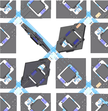
Figure 1: Several flaps of the active grid. The flow points out of the page. Starting from the top left flap in clockwise direction the flaps are set to 0º, 45º, 90º, and 45º. The side length of one flap is 11 cm, the black boxes in the flap center are servo motors, the blue rods are the grid support.

The autonomous active grid consists of 111 individually controllable flaps of dimensions 11 cm x 11 cm that rotate around their diagonal. This is different from the Makita-style grids, where the rows and columns of the flaps are mounted rigidly on rotating horizontal and vertical bars hideharu_realization_1991 . The angle of rotation can be set to any angle between $\pm 90{{}^{\circ}}$. The flow obstruction is smallest (flap parallel to the flow) at $0\text{\textdegree}$. At angles $\neq 0\text{\textdegree}$ one of the flap sides is facing the incoming flow, while the other side is facing away from the flow. The sign of the angles determines the side that is facing the flow, while the magnitude defines the deviation of the flap from the parallel position. As in a classical grid with rigid grid bars, wakes are formed that interact with each other downstream of the grid to form a turbulent flow field. The flexibility of the grid allows the superposition of larger structures onto those induced by the individual flaps. A detailed account of the autunomous active grid and the algorithm is given in Ref. griffin_control_2018 and briefly summarized here.

The algorithm updates the angle of each flap every 0.1s. Each time step starts with a random set of angles and convolves each of those angles with the history and a pre-defined kernel. The kernel is always defined by a certain shape (e.g. Gaussian), the spatial and temporal correlations (the number of neighbors and time-steps included in the convolution), and the desired mean absolute angle $\phi_{RMS}$. More complex kernel shapes require additional parameters. For the experiments presented here, a ’Long Tail’ kernel has been used, which reduces the correlation with neighboring flaps and therefore emphasizes the correlation of the angle with its own past.

This algorithm leads to dynamically evolving patches of more open and more closed flaps without periodicity. The typical time- and length scales of those patches are controlled by the spatial and temporal correlation lengths, $\sigma_{s}$ and $\sigma_{t}$, respectively, and the mean flap angle $\phi_{RMS}$ defines their mean amplitude. We describe the correlation as a box of dimensions $\sigma_{s}\times\sigma_{s}\times(\sigma_{t}\cdot U)$ and relate this volume $V_{\text{Corr}}$ to the energy injection scales $L=\int C(r)dr$ in Fig. 2 a. As expected, larger correlation volumes lead to larger energy injection scales, with a corresponding change in $R_{\lambda}$. $\sigma_{s}$ and $\sigma_{t}$ can be set independently, but to avoid a strongly inhomogeneous flow they are typically linked via the mean flow velocity $U$ forming a cubic correlation box: $\sigma_{t}\cdot U\approx\sigma_{s}$. This rule-of-thumb needs to be relaxed slightly to achieve $R_{\lambda}>3000$ leading to a correlation box that is elongated in the $\sigma_{t}$ direction.

The grid parameters can be distilled further into a grid Reynolds number. The relevant length scale is given by $\sqrt[3]{V_{\text{Corr}}}$, which corresponds to $\sigma_{s}$ in the case of a cubic correlation box. The fluctuating velocity is proportional to the mean flow velocity and the mean angle amplitudes $\phi_{RMS}$:

$$\text{Re}_{\text{Grid}}\sim\frac{\sqrt[3]{V_{\text{Corr}}}(\phi_{RMS}U)}{\nu},$$

where $U$ is the mean flow velocity of the VDTT and $\nu$ the kinematic viscosity. Fig. 2 b) shows that the a priori quantity $\text{Re}_{\text{Grid}}$ scales with the a posteriori $R_{\lambda}$ with deviations at $\text{Re}_{\text{Grid}}>10^{9}$. Each Dataset has been obtained by increasing $V_{\text{Corr}}$ while keeping the pressure (and therefore $\nu$ constant) as indicated in Tab. 1. We attribute the slight deviations at large $\text{Re}_{\text{Grid}}$ from a power law dependence to the fact that $L$ is approaching half the diameter of the measurement section. This is a natural limit for a sensible energy injection in any tunnel. We would like to add the word of caution that when approaching this limit, isotropy and homogeneity cannot be assumed easily anymore, which leads to said deviations from the isotropic relation $R_{\lambda}\sim\text{Re}_{\text{Grid}}^{\zeta}$ with $\zeta\approx 0.5$. Nevertheless, these data confirm that the active grid is indeed another ’knob’ to change $R_{\lambda}$ through the large scales.

Figure 2: (a) The correlation volume $V_{\text{corr}}=\sigma_{s}^{2}\sigma_{t}U$ influences the size of the largest scales $L$. (b) The grid Reynolds number defined as $\text{Re}_{\text{Grid}}=\sqrt[3]{V_{\text{corr}}}\phi_{RMS}U/\nu$ determines $R_{\lambda}$. The flattening of the individual Datasets indicate a limit to the increase of $R_{\lambda}$ through the active grid. The first spectrum of Dataset 1 is not shown, because $V_{\text{Corr}}$ is are not defined for a stationary, open grid.

II.2 Thermal Anemometry

More than a century after its invention comte-bellot_hot-wire_1976 , hot-wire anemometry remains the technique of choice to measure the energy spectrum of turbulent velocity fluctuations in a strong mean flow. Constant temperature anemometry is responsive to fluctuations up to very high frequencies. The sensing element’s resistance - and therefore its temperature - is kept constant by a feedback circuit. As long as the feedback circuit is fast enough, the thermal lag of the wire does not attenuate fluctuations faster than the thermal time scale of the wire. This comes at the expense of a mores complicated circuitry and frequency response.

The frequency response of CTA circuits has been studied extensively both through theoretical models and experimental testing. Freymuthfreymuth_frequency_1977 linearized a circuit with a single feedback amplifier of infinitely flat frequency response and analyzed its response to square and sine waves. He finds that the system can be modeled by a third-order ODE if the circuit responds faster than the wire, and the frequency response is optimal (flat over the entire range of frequencies) when the system response to a step perturbation by a single, slight overshoot (critically damped system). Perry & Morrison perry_study_1971 investigated more moderate amplifier gains and bridge imbalances in their study yielding similar results. Wood wood_method_1975 expanded the Perry & Morrison analysis, but considered a single-stage amplifier with a frequency-dependent response. Watmuff watmuff_investigation_1995 further expanded the model with multiple, non-ideal amplifier stages. He showed that at least two amplifier stages are necessary to model the real amplifier properly. This introduces two additional poles to the system and makes the frequency response more complicated. Samie et al. samie_modelling_2016 recently studied anemometry with sub-miniature probes in this model and compared it to a real CTA measurement. The results supported the further development of their in-house circuit, such that sub-miniature hot wire probes could be operated successfully on this CTA for the first time.

These theoretical attempts to predict the frequency response of a CTA circuit are accompanied by experimental approaches. Bonnet and de Roquefort bonnet_determination_1980 heated the wire periodically by a perturbation voltage as well as laser heating to determing the frequency response. Weiss et al. weiss_method_2001 used the aforementioned square wave test and interpreted its power spectrum as a measure for the frequency response curve. Hutchins et al. hutchins_direct_2015 exploited the well-defined frequency content of pipe flow at different operating pressures to obtain frequency response curves without artificial heating. They were able to create flows of almost identical Reynolds number, but different frequency content and could deduce the frequency-response curves for different circuits and wires. They compared several anemometer circuits and wires and found that the frequency responses are non-constant at frequencies as low as 500 Hz. For the combination of CTA circuit and wire used in the present study, they report an attenuation between 400 Hz and 7 kHz followed by a strong amplification of the signal. We therefore cannot assume a flat frequency response for our measurements and adress these effects below.

The energy spectrum measured by a hot wire is influenced by the effects of finite wire length. Length scales smaller than the sensor’s sensing lengths $l$ will be attenuated, but also larger wavenumbers are influenced. Wyngaard wyngaard_measurement_1968 used a Pao model spectrum pao_structure_1965 to investigate this attenuation of small scales. These results were reviewed in Ref. mckeon_velocity_2007 indicating that for $l/\eta=2$, the attenuation of the one-dimensional spectrum is still minimal at $k\eta\sim 0.3$, which was supported Ashok et al. ashok_hot-wire_2012 . Sadeghi et al. sadeghi_effects_2018 used sub-miniature hot wires (NSTAPs) as a benchmark and found that spatial filtering of the energy spectrum is minimal for $l/\eta<3.7$ at $k\eta<0.1$.

In this study we used conventional hot wires of sensing length 450 µm for pressures below 2 bar, as well as Nanoscale Thermal Anemometry Probes (NSTAP) of sensing length 30 µm provided by Princeton University with a Dantec Dynamics StreamWare CTA circuit. The NSTAP is a 100 nm thick, 2.5 µm wide, and 30 or 60 µm long free-standing platinum film supported by a silicon structure and soldered to the prongs of a Dantec hot wire. The production process and characteristics are detailed in Refs. fan_nanoscale_2015 ; kunkel_development_2006 ; bailey_turbulence_2010 ; vallikivi_fabrication_2014 . For the conventional hot wire $l/\eta<5$ in all cases and for the NSTAP $l/\eta<3$. Therefore, $\eta$ cannot be fully resolved in all cases. However, the bottleneck effect is typically found around $100\eta$. The aforementioned references show that we can regard the distortions due to finite wire length as minor in this part of the energy spectrum.

To summarize, the spatial resolution of our measurement instruments is sufficient to study the $R_{\lambda}$-dependence of the bottleneck effect. Nevertheless the nonlinear frequency response of the circuitry remains. Here we describe a procedure that takes the response into account and thus removes this systematic measurement error.

III Relative Spectra

Dataset	$R_{\lambda}$	$p$(bar)	$U$(m/s)	$u$(m/s)	Sensor	$L=\int C(r)dr$ (m)	$\eta$ (µm)	$f_{\eta}$(kHz)
1	193	1.5	2.75	0.04	Regular HW	0.12	277	9.9
1	500	1.5	2.41	0.14	Regular HW	0.19	139	17.3
1	690	1.5	2.41	0.18	Regular HW	0.23	127	19.0
1	735	1.5	2.65	0.19	Regular HW	0.27	127	20.9
1	757	1.5	2.43	0.20	Regular HW	0.24	116	20.9
1	989	1.5	2.72	0.22	Regular HW	0.32	120	22.7
1	1305	1.5	2.28	0.34	Regular HW	0.70	91	25.1
2	1308	5.95	3.64	0.20	NSTAP 1	0.19	37	98.4
2	1539	5.95	3.68	0.22	NSTAP 1	0.24	36	102.2
2	2385	5.97	3.64	0.35	NSTAP 1	0.33	28	130.0
2	2704	5.97	3.61	0.40	NSTAP 1	0.43	26	138.9
3	3641	14.62	3.75	0.44	NSTAP 2	0.38	10	375.0
3	3821	14.71	3.83	0.41	NSTAP 2	0.27	12	319.2
3	4247	14.65	3.97	0.53	NSTAP 2	0.54	9.2	431.5
3	5130	14.66	4.01	0.58	NSTAP 2	0.86	9.1	440.7

Table 1: Properties of all spectra. All spectra of a Dataset are distorted by the same function $T(f)$ describing the sensor- and instrument-induced bias. This is ensured by changing $R_{\lambda}$ only through large scales $L$ and fixing the position of the small scales in frequency space indicated by $f_{\eta}$. A reference spectrum has been chosen from each dataset, which is emboldened in this table.

III.1 The concept

As outlined above, systematic errors influence the energy spectra recorded with a hot-wire anemometer as outlined above. Formally, this means that the one-dimensional energy spectrum $E_{11}(f)$ is distorted by a frequency-dependent transfer function $T(f)$:

$$E_{M}(f)=E_{11}(f)\hphantom{}T(f)$$

$T(f)$ describes the effects of the thermal wire response, which depends on pressure and speed, and the reponse of the constant temperature anemometry circuit. Ideally, $T(f)$ is a constant over the whole range of relevant frequencies, but the evidence detailed above indicates a complex shape of amplification and attenuation of the signal. In this study we do not make any attempt to find $T(f)$. Instead, we control its effects by keeping $T(f)$ the same for several flows at different $R_{\lambda}$.

To ensure that the spectra only differ because of changes in the turbulent fluctuation and not because of the frequency response curve of the anemometer, we need to ensure that the response curve $T(f)$ is unaltered between spectra. We achieve this in two steps. The ambient pressure might influence the heat transfer of the wire and therefore $T(f)$. Furthermore, $T(f)$ is influenced by the CTA tuning (in particular the overheat), and the sensor itself. Therefore, we fix the ambient pressure within a set of spectra (a ’Dataset’) and measure using the same sensor and the same CTA settings.

The second step is to ensure that a given $k\eta$ is influenced by the same part of the frequency response curve $T(f)$. Thus, we need to fix the position of a spectral feature in frequency space. This means that the mean velocity $U$ must be the same within one Dataset. $T(f)$ mainly distorts the small-scale end of the spectrum freymuth_frequency_1977 ; hutchins_direct_2015 ; mckeon_velocity_2007 ; perry_study_1971 ; samie_modelling_2016 ; watmuff_investigation_1995 ; weiss_method_2001 ; wood_method_1975 , whose location in frequency space at a given $U$ is determined by the kinematic viscosity $\nu$. $\nu$ is fixed within a Dataset because the pressure remains constant.

We can, however, change the energy injection scale and thus the $R_{\lambda}$ with the autonomous active grid. This way we can conduct measurements at different $R_{\lambda}$. Ultimately, we can eliminate $T(f)$ by relating each spectrum to a reference spectrum:

$$\frac{E_{M}^{i}(f)}{E_{M}^{\text{Ref}}(f)} =\frac{E_{11}^{i}(f)T^{i}(f)}{E_{11}^{\text{Ref}}(f)T^{\text{Ref}}(f)}$$

$$=\frac{E_{11}^{i}(f)T(f)}{E_{11}^{\text{Ref}}(f)T(f)}=\frac{E_{11}(kU/2\pi)}{E_{11}^{\text{Ref}}(kU/2\pi)}.$$ (2)

In the following we call the ratio of a spectra divided by a reference spectrum in the frequncy domain, relative spectrum.

III.2 Results

We created three sets of spectra that have identical $T(f)$ each. We call these sets ‘Datasets‘. Tab. 1 shows important parameters for each spectrum. Note that $L$ changes significantly within a given dataset leading to changes in $R_{\lambda}$, while $f_{\eta}=U/\eta$ remains almost constant within the dataset. This indicates that we changed $R_{\lambda}$ only by increasing the large scales, while keeping all small-scale features of the spectrum at the same frequency $f_{F}$. For example, in Dataset 2, the peak of the spectral bump always lies at a frequency of $\sim 700$ Hz, whereas the beginning of the inertial range spans a factor of 4 in frequency (2 to 8 Hz). This exemplifies the excellent control over $R_{\lambda}$ permitted by the autonomous active grid as indicated in Fig. 2.

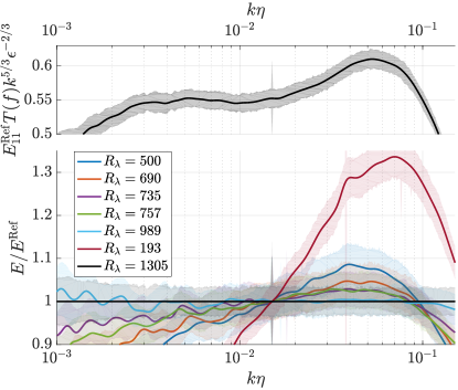
Figure 3: Reference spectrum at $R_{\lambda}=989$ (upper plot) and relative spectra from Dataset 1. The data have been collapsed at $k\eta=0.015$, which we defined as the beginning of the bottleneck region. We identified the peaks in the relative spectra with the bottleneck peak of the absolute spectra. The peak height decreased with increasing $R_{\lambda}$ and different spectra of similar $R_{\lambda}$ result in very similar relative spectra as expected. Furthermore, the slope of the spectrum at $k\eta<0.015$ seems to decrease with $R_{\lambda}$. The shaded areas are a measure of the noise level.

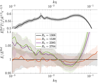
Figure 4: Reference spectrum at $R_{\lambda}=1308$ (upper plot) and relative spectra from Dataset 2. The trends in peak height and slope from Fig. 3 continue.

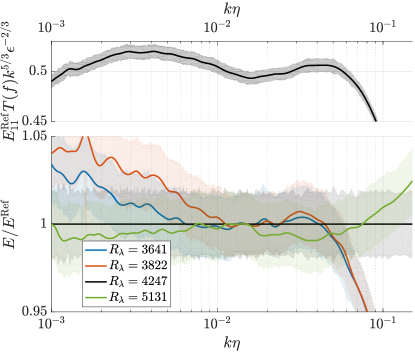
Figure 5: Reference spectrum at $R_{\lambda}=4247$ (upper plot) and relative spectra from Dataset 3. Unlike in Datasets 1 and 2, the beginning of the bottleneck region around $k\eta=0.015$ is identifiable in the relative spectra as a local extremum.

The lower graphs of Figs. 3 - 5 show the spectra from each of the respective datasets divided by the reference spectrum $E_{11}^{\text{Ref}}$. $E_{M}^{\text{Ref}}$ is plotted pre-compensated in the upper graphs of the respective figure. Note that the absolute spectra in the upper graphs are multiplied by an unknown transfer function $T(f)$ accounting for probe effects and therefore can not be used to realibly measure the features of the bottleneck. However, the relative curves are corrected and allow a measurement. The graphs are the result of a smoothing procedure and error estimate detailed in the appendix. In brief, the spectra were smoothed using a $1/f$ octave filtering and the error is related to the noise level removed by the smoothing procedure. The spectra have been divided by the reference spectrum in the frequency domain and collapsed at $k\eta=0.015$ afterwards to simplify interpretation.

While in Dataset 3 the beginning of the bottleneck region around $k\eta=0.015$ is accompanied by a change in the shape of the relative spectra, this point cannot be identified in the relative spectra of Datasets 1 and 2. The relative spectra seem to follow approximately straight lines in our semilogarithmic plot, i.e. $E_{11}/E_{11}^{\text{Ref}}\sim\zeta(R_{\lambda})\log(k\eta)$. The slope of these lines appears to become less steep with $R_{\lambda}$, leading to the prefactor $\zeta(R_{\lambda})$. In the following we concentrate on the bottleneck effect found at $k\eta>0.015$ for the remainder of this section.

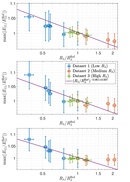
Figure 11: Bottleneck height as function of $R_{\lambda}/R_{\lambda}^{\text{Ref}}$ with different bottleneck definitions based on the height of the relative spectra at a fixed $k\eta$. The power law is the one found using the initial definition of the bottleneck height in Fig. 6. Upper graph: Bottleneck at $k\eta=0.03$, middle graph at $k\eta=0.04$, lower graph at $k\eta=0.046$ (as predicted by DNS). Datasets 1 and 2 still follow the trend found in the main part. Dataset 3 is not inconsistent with the claim of a constant bottleneck height at $R_{\lambda}>3000$.

The location of the spectral bump forming the bottleneck effect in relative spectra is not obvious. However, when considering the background noise, the peak location is not the major source of error. E.g. for $R_{\lambda}=1539$, all points between $0.015<k\eta<0.07$ are within the errorband at $k\eta=0.05$. We therefore define the extremum in the relative spectrum between $0.015<k\eta<0.08$ as the relative height $h$ of the bottleneck effect. This has the additional advantage to be independent of the errors in the estimate of $\eta$. To preclude biases from this definition, we repeat our analysis with different definitions of the relative bottleneck height in Fig. (11) in the appendix.

Finally, the measured bottleneck height cannot depend on which spectrum is chosen as reference. We have calculated the bottleneck height with all possible choices of $E_{11}^{\text{Ref}}$ and found our results to be largely independent of that choice (see Appendix for details).

Fig. 6 shows the bottleneck height - defined as above - as a function of $R_{\lambda}/R_{\lambda}^{\text{Ref}}$ within each dataset . The data shows a trend towards smaller peak heights in the relative spectrum with increasing $R_{\lambda}$. The data follows the numerical data we have compiled from various sources buaria_characteristics_2015 ; yeung_extreme_2015 ; buaria_extreme_2018 ; ishihara_energy_2016 . We have analyzed the data from Buaria et al. buaria_extreme_2018 at $R_{\lambda}$ up to 650 ($R_{\lambda}/R_{\lambda}^{\text{Ref}}<1$). The increased small-scale resolution in comparison to donzis_bottleneck_2010 seems to have no noticable impact on the bottleneck. Therefore, this data at is practically the same as the one used by Donzis & Sreenivasan donzis_bottleneck_2010 for our purposes. The data from $R_{\lambda}=1300$ ($R_{\lambda}/R_{\lambda}^{\text{Ref}}=1)$ was reported in Ref. buaria_characteristics_2015 . The numerical data at $R_{\lambda}/R_{\lambda}^{\text{Ref}}\approx 1.9$, which corresponds to $R_{\lambda}=2340$, is the highest $R_{\lambda}$ reported by Ishihara et al. ishihara_energy_2016 . The relative spectra of the numerical data were analyzed equivalently to the experimental data and the spectrum at $R_{\lambda}=1300$ was chosen as a reference spectrum.

When excluding the lowest $R_{\lambda}$, the experimental data is in agreement with the power law of

$$h\sim\left(R_{\lambda}/R_{\lambda}^{\text{Ref}}\right)^{-0.061\pm 0.007}.$$

The fit was obtained by a bootstrap procedure based on the error bars.

The spectrum at $R_{\lambda}=193$ follows the general trend of decreasing peak height with $R_{\lambda}$, but its peak differs substantially from the predictions. The absolute spectrum (not shown) exhibits no signs of a $5/3$-scaling, and consequently the bottleneck region cannot be clearly separated from the rest of the spectrum. This is substantially different from the other spectra, where the end of the integral range could always be observed in the absolute spectra and we therefore are not surprised that the relative spectrum at $R_{\lambda}=193$ deviates from the remainder of the data. This spectrum has consequently been ignored in our interpretation.

Further, we can change $R_{\lambda}$ only by a factor of 5 through the autonomous active grid. While Dataset 1 and 2 each feature a spectrum at the same $R_{\lambda}$, there is a gap between the highest $R_{\lambda}$ of Dataset 2 (2704) and the lowest of Dataset 3 (3641). To plot $h$ as a function of $R_{\lambda}$ alone, we use the aforementioned power law fit from Fig. 6, i.e. we assume $h(R_{\lambda}=3641)=h(R_{\lambda}=3641)(3641/2704)^{-0.061}$ to arrive at Fig. 7.

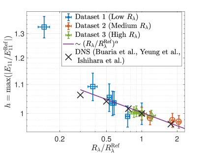
Figure 6: Bottleneck height relative to the reference spectrum for all datasets as a function of $R_{\lambda}/R_{\lambda}^{\text{Ref}}$. The reference spectra have bottleneck height 1. Numerical simulations from Buaria et al. buaria_extreme_2018 at $R_{\lambda}$ up to 650 ($R_{\lambda}/R_{\lambda}^{\text{Ref}}<1$), Buaria et al. buaria_characteristics_2015 ($R_{\lambda}=1$) and Ishihara ishihara_energy_2016 ($R_{\lambda}>1$ ) are added for reference. A power law is fitted to the experimental data with the lowest $R_{\lambda}/R_{\lambda}^{\text{Ref}}$ excluded. $(R_{\lambda}/R_{\lambda}^{\text{Ref}})^{-0.061\pm 0.007}$ is a good description of the experimental data over one decade of $R_{\lambda}$ (from 500 to 5000) and agrees with the numerical simulations as well. This power law is used in Fig. 7 to combine Datasets 2 and 3.

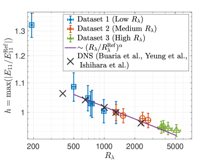
Figure 7: We have shifted Dataset 3 from Fig. 6 under the assumption of a power law $\sim\left(R_{\lambda}/R_{\lambda}^{\text{Ref}}\right)^{\alpha}$ with $\alpha=-0.061\pm 0.007$, i.e. the position of Dataset 3 with respect to the other Datasets is constructed artificially from the power law in Fig. 6. We have no physical justification for this power law and stress that the position of Dataset 3 in this figure is speculative.

IV Discussion

In this paper we studied the spectra of a turbulent wind tunnel flow of $R_{\lambda}$ between 193 and 5131. We have used regular hot-wires as well as NSTAPs with a state-of-the-art constant temperature anemometer to record single-point two-time statistics of the turbulent fluctuations, in particular energy spectra. However, such spectra can be heavily influenced by non-ideal frequency responses of the circuit. The frequency response is particularly complicated when operating sub-miniature wires like the NSTAP with a CTA samie_modelling_2016 ; hutchins_direct_2015 . A constant current anemometer (CCA) might perform better in this respect, because the frequency reponse is limited only by the thermal lag of the wire and no feedback loop is involved. Still, this comes at the expense of a variable wire temperature and -resistance.

In an attempt to interpret CTA data suffering from a non-flat frequency response, we consider energy spectra relative to a reference spectrum. Such an analysis significantly restricts the phenomena that can be observed. The bump in the energy spectrum at the transition from the inertial to the dissipation range can still be identified in the relative spectra as a local extremum beyond $k\eta=0.015.$

To the best of our knowledge, no other wind tunnel achieves $R_{\lambda}>5000$ in a gas. Moreover, we do not know of any other quantitative study of the scaling of the bottleneck effect with $R_{\lambda}$ in a laboratory experiment. We attribute this to the difficulties one faces when interpreting energy spectra from CTA measurements at relatively high frequencies: The spectrum is stronlgy influenced by the CTA circuitry and these influences are hard to quantify or eliminate.

With the aforementioned procedures we are able to extract information about the bottleneck effect from instrument-distorted hot wire spectra. We find indications that the bottleneck effect decreases up to $R_{\lambda}\sim 5000$. We fit a power law of $(R_{\lambda}/R_{\lambda}^{\text{Ref}})^{-\alpha}$ with $\alpha=0.061\pm 0.007$, which is close to the value of $(R_{\lambda})^{-0.04}$ found by Donzis & Sreenivasan donzis_bottleneck_2010 . Their numerical results are in general in good agreement with our experimental data, lending support to the experiment and data anlysis procedure. Our data equally supports Verma & Donzis verma_energy_2007 , who predict that the bottleneck scales as $h\sim 1-\gamma(1.5\log_{2}(R_{\lambda}))^{2/3}$.

We attempt to plot the relative bottleneck height as a function of $R_{\lambda}$ alone. This requires the assumption that the aforementioned power law holds and can be extrapolated. Such an assumption is highly speculative and the results should be considered as such.

We can not quantify the absolute height of the bottleneck bump. Yet, we can argue that if the relative spectra are still changing with $R_{\lambda}$ in the relevant region, the effect has not completely vanished. We can find a systematic decrease of the peak in the relative spectra for $R_{\lambda}<3000$. The data for $R_{\lambda}>3000$ in Dataset 3 is inconclusive. A small, decreasing trend can be found, consistent with the power law fit. However, the differences in height are so small compared to the error bars that the claim of a constant bottleneck height at $R_{\lambda}>3000$ would also be supported by the data, especially when considering alternative definitions of the bottleneck height in relative spectra as in Fig. 11 found in the appendix. This is not in contradiction to the atmospheric spectra mentioned above, as they have an even higher $R_{\lambda}$. Further, we note that a bottleneck effect might not show up as a peak in a $5/3$-compensated spectrum, yet might be present when compensating by an intermittency-corrected slope $-(5/3+\beta)$. In this case, the bottleneck effect would still be visible in the relative spectrum. However, the claim that the bottleneck height does not change with $R_{\lambda}$ for $R_{\lambda}>3000$ is not ruled out by the data.

As far as this study is concerned, the data matches the predictions of Verma & Donzis verma_energy_2007 : The bottleneck height decreases with increasing $R_{\lambda}$, but relatively high $R_{\lambda}$ are necessary to make the effect vanish completely. Based on nonlinear and nonlocal shell-to-shell energy transfer Verma & Donzis verma_energy_2007 estimate that the bottleneck is basically absent for $R_{\lambda}>10^{4}$, but acknowledge that this might be an overestimate. While lending support to existing studies of the bottleneck effect, especially donzis_bottleneck_2010 and theories that incorporate a $R_{\lambda}$-dependence of the peak height, an investigation of the effect in terms of absolute measurements of spectra seems necessary to confirm these claims experimentally. With subminiature probes of low thermal lag, such a study might be possible with a constant current anemometer, whose frequency response is intriniscally more simple.

V Conclusions

Hot-wire measurements of high-wavenumber parts of the energy spectrum in a turbulent flow such as the bottleneck effect are distorted by non-flat frequency responses typical for constant temperature anemometers. When the experiment allows for a change in $R_{\lambda}$ through the forcing mechanism alone, the $R_{\lambda}$-dependence at such high wavenumbers can be investigated. We have used an active grid to fix the frequency at which the bottleneck effect occurs. Thereby the bottleneck effect was always subject to the same systematic errors. By considering spectra relative to a reference spectrum, we found a $R_{\lambda}$-scaling of the bottleneck effect.

We have found indications that the bottleneck effect gets weaker with increasing $R_{\lambda}$. The data are very similar to the results of DNS donzis_bottleneck_2010 and a theory verma_energy_2007 . $R_{\lambda}$ exceeds 5000 in the VDTT with an autonomous active grid, which is unprecedented in any wind tunnel. At $R_{\lambda}>3000$ our data supports a further decrease of the bottleneck height with $R_{\lambda}$ as well as a constant or absent bottleneck.

Appendix A A brief description of the wind tunnel

The VDTT consists of two 11.7 m long straight cylindrical tubes connected by two elbows of center-line radius of 1.75 m. The tunnel was filled with sulfur-hexaflouride (SF6) at pressures between 1.5 and 15 bar for the measurements presented here.

The flow is propelled by a fan rotating at up to 24 Hz creating mean flow speeds of up to 5.5 m/s. It passes the first elbow and enters a heat exchanger, which removes any turbulent energy dissipated into heat and thus keeps the temperature in the tunnel constant. The rectangular cross-section of the heat exchanger is smoothly adapted to the tunnels circular geometry by contractions. The vertical slots of the heat exchanger are expected to destroy large-scales structure present in the flow. After the heat exchanger, the flow passes an 80 cm long expansion, which adapts it to the measurement section. While passing this expansion the flow is stabilized and homogenized by three consecutive meshes of ascending spacing. The flow enters a 9 m long measurement section through an 104 cm high active grid, which is directly followed by a 70 cm long expansion to the measurement section’s height of 117 cm. The measurement section is followed by another elbow and enters a second measurement section through another sequence of three meshes before being accelerated again by the fan.

Appendix B Data Acquisition and Analysis Procedure

The NSTAPs were operated following largely fan_high_2017 using a Dantec StreamLine 90C10 module within a 90N10 frame. The CTA bridge was set to a 1:1 ratio and the overheat is determined by an external resistor $R_{\text{ext}}$ connected to the system. Typical overheat ratios $R_{\text{ext}}/R_{\text{Probe}}$ were 1.2-1.3, where $R_{\text{Probe}}\sim 100\,\Omega$ denotes the probe cold resistance. The Dantec wires were used in a 1:20 bridge utilizing the internal automatics to set the overheat. The data was acquired in the following procedure: The hot wire frequency response and proper operation was tested on a very basic level using the square wave test built into the Dantec CTA-system. The hot-wire system was calibrated by scanning a range of mean flow speeds set by the fan frequency in the tunnel. We determined the mean flow speed through the differential pressure between a pitot tube and a static pressure probe. The differential pressure was picked up by a Siemens SITRANS differential pressure transfucer/ We chose ~ 20 calibration points spaced by ~ 0.1 m/s. The probe voltage was recorded for 60 seconds along with the mean pressure difference, a voltage-velocity curve was calculated, and King’s law was fitted to the data. In between calibration points we waited for 45 seconds for the mean flow to become stationary. The data was recorded with a National Instruments NI PCI-6123 16-bit DAQ-Card at sampling rates of 60 or 200 kHz. Higher sampling rates were used for NSTAP measurements, where the CTA analog low-pass filter was set to 100 kHz. When using standard hot wires, the filter frequency was set to 30 kHz and the data was sampled at 60 kHz. The data was recorded in segments of 6 million voltage samples, each saved to disk in a 16-bit binary format.

We shall briefly outline the initial data analysis procedure used to obtain essential turbulence statistics as well as the power spectrum. Each of the following steps was carried out on each segment and the results were averaged over all files in the end. We used King’s law with parameters obtained form the calibration data to convert the voltages to velocities. Note that the shape of the energy-frequency spectrum is independent of the calibration, which is only required to obtain its absolute value. Because the analog filtering was not sufficient to filter out all noise, we low-pass filtered the data digitally using a sinc-Filter in forward and reverse directions. This introduces edge effects, which we remove by cutting the first and last 60 points of the time series. We then subtract the mean $U$ from the velocity time series to obtain a time series of $u$. The remaining analysis is performed on this filtered dataset. The power spectra were calculated using MATLB’s fft function, which is based on the FFTW-package . We calculate the correlation function using MATLAB’s xcorr function, which itself relies on the aforementioned fourier transform procedure as well as structure functions of order 1 to 8. Finally, we obtain histograms of velocity and voltage. We use Taylor’s Hypothesis, which assumes that a one-dimensional velocity field can be obtained from a time series by multiplying the time increments by the mean velocity: $\Delta x=\Delta t\cdot U$. The power spectra are normalized using the assumption that $\int E(k)dk=u^{2}$.

We routinely calculate basic turbulence quantities in different ways and check the results for consistency. The quantites $R_{\lambda}$, and $\eta$ depend on the mean energy dissipation rate $\varepsilon$, which we measure using the third-order structure function $S_{3}(r)=\langle(u(x+r)-u(x))^{3}\rangle=4/5(\varepsilon r)$. The last step follows from the Navier-Stokes equations and is also predicted by Kolmogorov’s 1941 theory. In practice we estimate $\varepsilon=\max(5/4\ S_{3}/r)$ and check the result with $\varepsilon=15\nu\int k^{2}E(k)dk$, and $\varepsilon=\max(S_{2}^{3/2}/r)$. The integral length scale is calculated as $L=\int_{0}^{\infty}C(r)dr$, where $C(r)=\langle u(x+r)u(x)\rangle$ is the velocity auto-correlation function. Its error mainly stems from the ambiguous choice of the upper integration limit, which leads to a relative error about 10% in $L$.

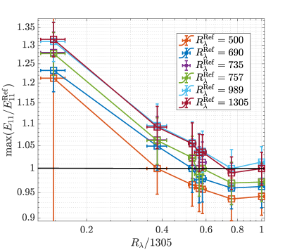
Figure 8: The bottleneck height in Dataset 1 with different choices of $E_{11}^{\text{Ref}}$. If the analysis is independent of the choice of reference spectrum, the graphs are parallel in this representation. Note that the reference spectrum always has bottleneck height 1.

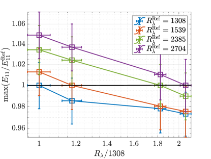
Figure 9: Same as Fig. 8 for Dataset 2

Appendix C Calculation and Cross-check of Relative Spectra

To obtain relative spectra, the initial spectrum consisting of 3 million points was downsampled to 50 000 logarithmically spaced datapoints. To remove the noise from these spectra, we have smoothed them using a fractional octave smoothing algorithm. It multiplies the spectrum at each frequency with a Gaussian centered around the current frequency $f_{i}$ with a width of $\sigma_{i}=(f_{i}/n)/\pi$, where $n$ determines the smoothing level. Therefore, the smoothing window is larger for higher frequencies. To estimate the noise level in the spectrum and the associated statistical error, we consider the data within $3\sigma_{i}$ of each frequency. We estimate the standard error as $\delta=3\sqrt{\text{Var}/N}$, where $N$ is the number of points considered and Var denotes their variance. Finally, the compensated spectra are calculated as $\psi(k)=E_{11}(k)k^{5/3}\varepsilon^{-2/3}$, which can be written as $\psi(f)$ by Taylor’s Hypothesis. Finally, we divide the $i$-th spectrum in a dataset by the reference spectrum: $\psi_{i}(f)/\psi_{\text{Ref}}(f)$. The result is normalized at $k\eta=0.015$ to remove offsets introduced by uncertainties in $\varepsilon$ and to simplify comparisons.

An important cross-check of the technique is its independence from the choice of reference spectrum. To this end we have calculated the bottleneck effect according to the analysis outlined above for all possible choices of reference spectra. The results are shown in Figs. 8-10. They show the peak height in the relative spectra as a function of $R_{\lambda}/R_{\lambda}^{\text{Ref}}$. $R_{\lambda}/R_{\lambda}^{\text{Ref}}$ has been normalized to the value that was chosen in the main part of the paper to increase the clarity of the figures. If the analysis is independent of the choice of reference spectrum $E_{11}^{\text{Ref}}$, a different choice $E_{11}^{\prime\text{Ref}}$, should move the resulting curve by a factor of $E_{11}^{\text{Ref}}/E_{11}^{\text{Ref}}$ upwards and $R_{\lambda}^{\text{Ref}}/R_{\lambda}^{\prime\text{Ref}}$ to the right. The latter is trivial and has been removed from Figs. 8-10 by the additional normalization. Thus, if the spectra are independent of the choice of reference spectrum, the bottleneck curves should be parallel. Figs. 8-10 show that this is valid in good approximation showing that the analysis is largely independent of the choice of reference spectrum within a dataset.

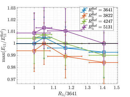
Figure 10: Same as Fig. 8 for Dataset 3

References

- (1) Ashok, A., Bailey, S.C.C., Hultmark, M., Smits, A.J.: Hot-Wire Spatial Resolution Effects in Measurements of Grid-Generated Turbulence. Experiments in Fluids 53(6), 1713–1722 (2012). DOI 10.1007/s00348-012-1382-5
- (2) Bailey, S.C.C., Kunkel, G.J., Hultmark, M., Vallikivi, M., Hill, J.P., Meyer, K.A., Tsay, C., Arnold, C.B., Smits, A.J.: Turbulence Measurements using a Nanoscale Thermal Anemometry Probe. Journal of Fluid Mechanics 663, 160–179 (2010). DOI 10.1017/S0022112010003447
- (3) Bodenschatz, E., Bewley, G.P., Nobach, H., Sinhuber, M., Xu, H.: Variable Density Turbulence Tunnel Facility. Review of Scientific Instruments 85(9), 093908 (2014). DOI 10.1063/1.4896138
- (4) Bonnet, J.P., Alziary de Roquefort, T.: Determination and Optimization of Frequency Response of Constant Temperature Hot-Wire Anemometers in Supersonic Flows. Review of Scientific Instruments 51(2), 234–239 (1980). DOI 10.1063/1.1136180
- (5) Bourgoin, M., Baudet, C., Kharche, S., Mordant, N., Vandenberghe, T., Sumbekova, S., Stelzenmuller, N., Aliseda, A., Gibert, M., Roche, P.E., Volk, R., Barois, T., Caballero, M.L., Chevillard, L., Pinton, J.F., Fiabane, L., Delville, J., Fourment, C., Bouha, A., Danaila, L., Bodenschatz, E., Bewley, G., Sinhuber, M., Segalini, A., Örlu, R., Torrano, I., Mantik, J., Guariglia, D., Uruba, V., Skala, V., Puczylowski, J., Peinke, J.: Investigation of the small-scale statistics of turbulence in the Modane S1MA wind tunnel 9(2), 269–281. DOI 10.1007/s13272-017-0254-3.
- (6) Buaria, D., Pumir, A., Bodenschatz, E., Yeung, P.K.: Extreme velocity gradients in turbulent flows. under Review
- (7) Buaria, D., Sawford, B.L., Yeung, P.K.: Characteristics of backward and forward two-particle relative dispersion in turbulence at different Reynolds numbers. Physics of Fluids 27(10), 105101. DOI 10.1063/1.4931602.
- (8) Comte-Bellot, G.: Hot-wire anemometry 8(1), 209–231. DOI 10.1146/annurev.fl.08.010176.001233.
- (9) Dobler, W., Haugen, N.E.L., Yousef, T.A., Brandenburg, A.: Bottleneck Effect in Three-Dimensional Turbulence Simulations. Physical Review E 68(2) (2003). DOI 10.1103/PhysRevE.68.026304
- (10) Donzis, D.A., Sreenivasan, K.R.: The best Bottleneck Effect and the Kolmogorov Constant in Isotropic Turbulence. Journal of Fluid Mechanics 657, 171–188 (2010). DOI 10.1017/S0022112010001400
- (11) Falkovich, G.: Bottleneck Phenomenon in Developed Turbulence. Physics of Fluids 6(4), 1411–1414 (1994). DOI 10.1063/1.868255
- (12) Fan, Y.: High Resolution Instrumentation for Flow Measurements. Thesis, Princeton University, Princeton, NJ, USA (2017)
- (13) Fan, Y., Arwatz, G., Van Buren, T.W., Hoffman, D.E., Hultmark, M.: Nanoscale Sensing Devices for Turbulence Measurements. Experiments in Fluids 56(138) (2015). DOI 10.1007/s00348-015-2000-0
- (14) Fefferman, C.L.: Existence and smoothness of the navier-stokes equation 57, 67. Citation Key: fefferman2006existence
- (15) Freymuth, P.: Frequency Response and Electronic Testing for Constant-Temperature Hot-Wire Anemometers. J. Phys. E: Sci. Instrum. 10(7), 705 (1977). DOI 10.1088/0022-3735/10/7/012
- (16) Frisch, U., Kurien, S., Pandit, R., Pauls, W., Ray, S.S., Wirth, A., Zhu, J.Z.: Hyperviscosity, Galerkin Truncation, and Bottlenecks in Turbulence. Phys. Rev. Lett. 101(14), 144501 (2008). DOI 10.1103/PhysRevLett.101.144501
- (17) Griffin, K.P., Wei, N.J., Bodenschatz, E., Bewley, G.P.: Control of Long-Range Correlations in Turbulence. Experiments in Fluids under review (2018)
- (18) Gulitski, G., Kholmyansky, M., Kinzelbach, W., Lüthi, B., Tsinober, A., Yorish, S.: Velocity and Temperature Derivatives in high-Reynolds-number Turbulent Flows in the Atmospheric Surface Layer. Part 1. Facilities, methods and some general results. Journal of Fluid Mechanics 589 (2007). DOI 10.1017/S0022112007007495
- (19) Hideharu, M.: Realization of a Large-Scale Turbulence Field in a Small Wind Tunnel. Fluid Dynamics Research 8(1), 53–64 (1991). DOI 10.1016/0169-5983(91)90030-M
- (20) Hutchins, N., Monty, J.P., Hultmark, M., Smits, A.J.: A Direct Measure of the Frequency Response of Hot-Wire Anemometers: Temporal Resolution Issues in Wall-Bounded Turbulence. Experiments in Fluids 56(18) (2015). DOI 10.1007/s00348-014-1856-8
- (21) Ishihara, T., Kaneda, Y., Yokokawa, M., Itakura, K., Uno, A.: Energy Spectrum in the Near Dissipation Range of High Resolution Direct Numerical Simulation of Turbulence. Journal of the Physical Society of Japan 74(5), 1464–1471 (2005). DOI 10.1143/JPSJ.74.1464
- (22) Ishihara, T., Morishita, K., Yokokawa, M., Uno, A., Kaneda, Y.: Energy Spectrum in High-Resolution Direct Numerical Simulations of Turbulence. Physical Review Fluids 1(8) (2016). DOI 10.1103/PhysRevFluids.1.082403
- (23) Khurshid, S., Donzis, D.A., Sreenivasan, K.R.: Energy Spectrum in the Dissipation Range. Physical Review Fluids 3(8) (2018). DOI 10.1103/PhysRevFluids.3.082601
- (24) Kolmogorov, A.: The Local Structure of Turbulence in Incompressible Viscous Fluid for Very Large Reynolds Numbers. Akademiia Nauk SSSR Doklady 30, 301–305
- (25) Kunkel, G., Arnold, C., Smits, A.: Development of NSTAP: Nanoscale Thermal Anemometry Probe. American Institute of Aeronautics and Astronautics (2006). DOI 10.2514/6.2006-3718
- (26) Kurien, S., Taylor, M.A., Matsumoto, T.: Cascade Time Scales for Energy and Helicity in Homogeneous Isotropic Turbulence. Phys. Rev. E 69(6), 066313 (2004). DOI 10.1103/PhysRevE.69.066313
- (27) Lohse, D., Mueller-Groeling, A.: Bottleneck effects in turbulence: Scaling phenomena in r- versus p-space. Physical Review Letters 74(10), 1747–1750. DOI 10.1103/PhysRevLett.74.1747.
- (28) McKeon, B., Comte-Bellot, G., Foss, J., Westerweel, J., Scarano, F., Tropea, C., Meyers, J., Lee, J., Cavone, A., Schodl, R., Koochesfahani, M., Andreopoulos, Y., Dahm, W., Mullin, J., Wallace, J., Vukoslavčević, P., Morris, S., Pardyjak, E., Cuerva, A.: Velocity, Vorticity, and Mach Number. In: C. Tropea, A.L. Yarin, J.F. Foss (eds.) Springer Handbook of Experimental Fluid Mechanics, pp. 215–471. Springer Berlin Heidelberg, Berlin, Heidelberg (2007). DOI 10.1007/978-3-540-30299-5_5
- (29) Pao, Y.: Structure of Turbulent Velocity and Scalar Fields at Large Wavenumbers. The Physics of Fluids 8(6), 1063–1075. DOI 10.1063/1.1761356.
- (30) Perry, A.E., Morrison, G.L.: A Study of the Constant-Temperature Hot-Wire Anemometer. Journal of Fluid Mechanics 47(3), 577 (1971). DOI 10.1017/S0022112071001241
- (31) Pietropinto, S., Poulain, C., Baudet, C., Castaing, B., Chabaud, B., Gagne, Y., Hebral, B., Ladam, Y., Lebrun, P., Pirotte, O., Roche, P.: Superconducting Instrumentation for high Reynolds Turbulence Experiments with low Temperature gaseous Helium. Physica C: Superconductivity 386, 512–516. DOI 10.1016/S0921-4534(02)02115-9.
- (32) Rousset, B., Bonnay, P., Diribarne, P., Girard, A., Poncet, J.M., Herbert, E., Salort, J., Baudet, C., Castaing, B., Chevillard, L., Daviaud, F., Dubrulle, B., Gagne, Y., Gibert, M., Hebral, B., Lehner, T., Roche, P.E., Saint-Michel, B., Bon Mardion, M.: Superfluid high REynolds von Kármán experiment. Review of Scientific Instruments 85(10), 103908 (2014). DOI 10.1063/1.4897542
- (33) Saddoughi, S.G., Veeravalli, S.V.: Local Isotropy in Turbulent Boundary Layers at high Reynolds number. Journal of Fluid Mechanics 268, 333 (1994). DOI 10.1017/S0022112094001370
- (34) Sadeghi, H., Lavoie, P., Pollard, A.: Effects of Finite Hot-Wire Spatial Resolution on Turbulence Statistics and Velocity Spectra in a Round Turbulent Free Jet. Experiments in Fluids 59(40) (2018). DOI 10.1007/s00348-017-2486-8
- (35) Saint-Michel, B., Herbert, E., Salort, J., Baudet, C., Bon Mardion, M., Bonnay, P., Bourgoin, M., Castaing, B., Chevillard, L., Daviaud, F., Diribarne, P., Dubrulle, B., Gagne, Y., Gibert, M., Girard, A., Hébral, B., Lehner, T., Rousset, B., SHREK Collaboration: Probing Quantum and Classical Turbulence Analogy in von Kármán liquid Helium, Nitrogen, and Water Experiments. Physics of Fluids 26(12), 125109 (2014). DOI 10.1063/1.4904378
- (36) Salort, J., Chabaud, B., Leveque, E., Roche, P.E.: Energy cascade and the four-fifths law in superfluid turbulence. Europhysics Letters 97(3), 34006. DOI 10.1209/0295-5075/97/34006.
- (37) Samie, M., Watmuff, J.H., Van Buren, T., Hutchins, N., Marusic, I., Hultmark, M., Smits, A.J.: Modelling and Operation of Sub-Miniature Constant Temperature Hot-Wire Anemometry. Measurement Science and Technology 27, 125301 (2016). DOI 10.1088/0957-0233/27/12/125301
- (38) She, Z.S., Jackson, E.: On the Universal Form of Energy Spectra in Fully Developed Turbulence. Physics of Fluids A: Fluid Dynamics 5(7), 1526–1528 (1993). DOI 10.1063/1.858591
- (39) Sinhuber, M., Bewley, G.P., Bodenschatz, E.: Dissipative Effects on Inertial-Range Statistics at High Reynolds Numbers. Phys. Rev. Lett. 119(13), 134502. DOI 10.1103/PhysRevLett.119.134502. Citation Key: PhysRevLett.119.134502 bibtex[publisher=American Physical Society;numpages=5]
- (40) Sinhuber, M., Bodenschatz, E., Bewley, G.P.: Decay of Turbulence at High Reynolds Numbers. Physical Review Letters 114(3) (2015). DOI 10.1103/PhysRevLett.114.034501
- (41) Sreenivasan, K.R., Dhruva, B.: Is There Scaling in High-Reynolds-Number Turbulence? Progress of Theoretical Physics Supplement 130, 103–120 (1998). DOI 10.1143/PTPS.130.103
- (42) Taylor, G.I.: The Spectrum of Turbulence. Proc R Soc Lond A Math Phys Sci 164(919), 476. DOI 10.1098/rspa.1938.0032.
- (43) Taylor, G.I.: Statistical Theory of Turbulence. Proc R Soc Lond A Math Phys Sci 151(873), 421. DOI 10.1098/rspa.1935.0158.
- (44) Tsuji, Y.: Intermittency Effect on Energy Spectrum in High-Reynolds Number Turbulence. Physics of Fluids 16, L43–L46 (2004). DOI 10.1063/1.1689931
- (45) Vallikivi, M., Smits, A.J.: Fabrication and Characterization of a Novel Nanoscale Thermal Anemometry Probe. Journal of Microelectromechanical Systems 23(4), 899–907 (2014). DOI 10.1109/JMEMS.2014.2299276
- (46) Verma, M.K., Ayyer, A., Debliquy, O., Kumar, S., Chandra, A.V.: Local shell-to-shell energy transfer via nonlocal interactions in fluid turbulence. Pramana - J Phys 65(2), 297. DOI 10.1007/BF02898618.
- (47) Verma, M.K., Donzis, D.: Energy Transfer and Bottleneck Effect in Turbulence. Journal of Physics A: Mathematical and Theoretical 40(16), 4401–4412 (2007). DOI 10.1088/1751-8113/40/16/010
- (48) Watmuff, J.H.: An Investigation of the Constant-Temperature Hot-Wire Anemometer. Experimental Thermal and Fluid Science 11, 117–134 (1995). DOI 10.1016/0894-1777(94)00137-W
- (49) Weiss, J., Knauss, H., Wagner, S.: Method for the Determination of Frequency Response and Signal to Noise Ratio for Constant-Temperature Hot-Wire Anemometers. Review of Scientific Instruments 72, 1904 (2001). DOI 10.1063/1.1347970
- (50) Wood, N.B.: A Method for Determination and Control of the Frequency Response of the Constant-Temperature Hot-Wire Anemometer. Journal of Fluid Mechanics 67(4), 769 (1975). DOI 10.1017/S0022112075000602
- (51) Wyngaard, J.C.: Measurement of Small-Scale Turbulence Structure with Hot Wires. Journal of Physics E: Scientific Instruments 1, 1105–1108 (1968). DOI 10.1088/0022-3735/1/11/310
- (52) Yakhot, V., Zakharov, V.: Hidden conservation laws in hydrodynamics; energy and dissipation rate fluctuation spectra in strong turbulence. Physica D: Nonlinear Phenomena 64(4), 379–394. DOI 10.1016/0167-2789(93)90050-B.
- (53) Yeung, P.K., Sreenivasan, K.R., Pope, S.B.: Effects of Finite Spatial and Temporal Resolution in Direct Numerical Simulations of Incompressible Isotropic Turbulence. Physical Review Fluids 3(6) (2018). DOI 10.1103/PhysRevFluids.3.064603
- (54) Yeung, P.K., Zhai, X.M., Sreenivasan, K.R.: Extreme events in computational turbulence. Proc Natl Acad Sci USA 112(41), 12633. DOI 10.1073/pnas.1517368112.