An estimate of approximation
of a matrix-valued function
by an interpolation polynomial

Abstract.

Let $A$ be a square complex matrix, $z_{1}$, …, $z_{n}\in\mathbb{C}$ be (possibly repetitive) points of interpolation, $f$ be a function analytic in a neighborhood of the convex hull of the union of the spectrum of $A$ and the points $z_{1}$, …, $z_{n}$, and $p$ be the interpolation polynomial of $f$ constructed by the points $z_{1}$, …, $z_{n}$. It is proved that under these assumptions

$$\lVert f(A)-p(A)\rVert\leq\frac{1}{n!}\max_{\begin{subarray}{c}t\in[0,1]\\ \mu\in\operatorname{co}\{z_{1},z_{2},\dots,z_{n}\}\end{subarray}}\bigl{\lVert}\Omega(A)f^{{(n)}}\bigl{(}(1-t)\mu\mathbf{1}+tA\bigr{)}\bigr{\rVert},$$

where $\Omega(z)=\prod_{k=1}^{n}(z-z_{k})$ and the symbol $\operatorname{co}$ means the convex hull.

Introduction

An approximate calculation of analytic functions of matrices [4, 12] arises in many applications. One of the often used methods for the approximate calculation of a function $f$ of a large matrix $A$ is the replacement of $f$ by its polynomial approximation $p$. For the approximation by the Taylor polynomial, it is known a good estimate of accuracy [16], see Corollary 2. In this paper, we propose an estimate of the norm $\lVert f(A)-p(A)\rVert$, which is a generalization of the estimate from [16] for the case when $p$ is an interpolation polynomial of $f$. This estimate may help to choose an interpolation polynomial for an approximate calculation of a matrix function in an optimal way. Our estimate can be considered as a matrix analogue of the estimate [3, Theorem 3.1.1]

$$|f(z)-p(z)|\leq\frac{1}{n!}|\Omega(z)|\max_{\lambda\in\operatorname{co}\{z_{1},z_{2},\dots,z_{n},\,z\}}|f^{(n)}(\lambda)|,$$

where

$$\Omega(z)=\prod_{k=1}^{n}(z-z_{k}),$$

for the difference between an analytic function $f$ and its interpolation polynomial $p$ with respect to the points of interpolation $z_{1}$, …, $z_{n}$ provided that $f$ is analytic in a neighborhood of the convex hull of the points $z_{1}$, …, $z_{n}$ and $z$.

It is known many estimates of $\lVert f(A)\rVert$, see, e.g., [2, 7, 8, 9, 11, 15, 17, 18, 19]. All of them can be equivalently written as estimates of $\lVert f(A)-p(A)\rVert$, see, e.g., [10, Theorem 11.2.2]. The difference between these estimates and the proposed one (Theorem 1) is that the latter is adapted for the approximation by an interpolation polynomial.

In Section 1, we prove our estimate (Theorem 1) and describe some of its variants for the case of the matrix exponent. In Section 2, we give a numerical application.

1. The estimate

Theorem 1.

Let $A$ be a square complex matrix, $z_{1}$, …, $z_{n}\in\mathbb{C}$ be arbitrary (possibly repetitive) points of interpolation, $f$ be an analytic function defined in a neighborhood of the convex hull of the union of the spectrum of $A$ and the points $z_{1}$, …, $z_{n}$, and $p$ be the interpolation polynomial of $f$ constructed by the points $z_{1}$, …, $z_{n}$ (taking into account their multiplicities). Then (for any norm on the space of matrices)

$$\lVert f(A)-p(A)\rVert\leq\frac{1}{n!}\max_{\begin{subarray}{c}t\in[0,1]\\ \mu\in\operatorname{co}\{z_{1},z_{2},\dots,z_{n}\}\end{subarray}}\bigl{\lVert}\Omega(A)f^{{(n)}}\bigl{(}(1-t)\mu\mathbf{1}+tA\bigr{)}\bigr{\rVert},$$

where $\mathbf{1}$ is the identity matrix, the symbol $\operatorname{co}$ means the convex hull, and

$$\Omega(z)=\prod_{k=1}^{n}(z-z_{k}).$$

Proof.

It is well-known (see, e.g., [3, Theorem 3.4.1] or [6, formula (52)]) that

$$f(z)-p(z)=\Omega(z)f[z_{1},z_{2},\dots,z_{n},z],$$

where $f[z_{1},z_{2},\dots,z_{n},z]$ is the divided difference [3, 6, 14]. On the other hand, by [6, formula (47)], we have

$$f[z_{1},z_{2},\dots,z_{n},z]=\int_{0}^{1}\int_{0}^{t_{1}}\dots\int_{0}^{t_{n-1}}f^{(n)}\bigl{(}z_{1}+(z_{2}-z_{1})t_{1}+\dots{\\ }+(z_{n}-z_{n-1})t_{n-1}+(z-z_{n})t_{n}\bigr{)}\,dt_{n}dt_{n-1}\dots dt_{1}.$$ (1)

Or

$$f[z_{1},z_{2},\dots,z_{n},z]=\int_{0}^{1}\int_{0}^{t_{1}}\dots\int_{0}^{t_{n-1}}f^{{(n)}}\bigl{(}(1-t_{1})z_{1}+(t_{1}-t_{2})z_{2}+\dots{\\ }+(t_{n-1}-t_{n})z_{n}+t_{n}z\bigr{)}\,dt_{n}dt_{n-1}\dots dt_{1}.$$

Clearly, the complex numbers

$$(1-t_{1})z_{1}+(t_{1}-t_{2})z_{2}+\dots+(t_{n-1}-t_{n})z_{n}+t_{n}z$$

form the convex hull of the set $\{z_{1},z_{2},\dots,z_{n},z\}$ when $t_{1},\dots,t_{n}$ run through the set specified by the inequalities $0\leq t_{n}\leq\dots\leq t_{1}\leq 1$. Thus, considering integral (1), we use the fact that $f^{(n)}$ is defined on the convex hull of the points $z_{1}$, …, $z_{n}$, and $z$.

Substituting $A$ for $z$ into the previous formulas (thus, we assume that any point of the spectrum of $A$ can be taken as $z$, which can be done, since $f$ is analytic in a neighborhood of the convex hull of the union of the spectrum of $A$ and the points $z_{1}$, …, $z_{n}$), we obtain

$$f(A)-p(A)=\Omega(A)\int_{0}^{1}\int_{0}^{t_{1}}\dots\int_{0}^{t_{n-1}}f^{{(n)}}\bigl{(}(1-t_{1})z_{1}\mathbf{1}+(t_{1}-t_{2})z_{2}\mathbf{1}+\dots{\\ }+(t_{n-1}-t_{n})z_{n}\mathbf{1}+t_{n}A\bigr{)}\,dt_{n}dt_{n-1}\dots dt_{1}.$$

Let $\xi$ be a linear functional on the space of matrices (equipped by an arbitrary norm) such that $\lVert\xi\rVert=1$ and

$$\lVert f(A)-p(A)\rVert=\xi\bigl{(}f(A)-p(A)\bigr{)}.$$

Such a functional exists by the Hahn-Banach theorem [13, Theorem 2.7.4]. Then we have the estimate

$$\begin{split}\lVert f(A)-p(A)\rVert&=\xi\biggl{(}\int_{0}^{1}\int_{0}^{t_{1}}\dots\int_{0}^{t_{n-1}}\Omega(A)f^{{(n)}}\bigl{(}(1-t_{1})z_{1}\mathbf{1}+\dots\\ &\phantom{fghfg}+(t_{n-1}-t_{n})z_{n}\mathbf{1}+t_{n}A\bigr{)}\,dt_{n}dt_{n-1}\dots dt_{1}\biggr{)}\\ &\leq\biggl{\lVert}\int_{0}^{1}\int_{0}^{t_{1}}\dots\int_{0}^{t_{n-1}}\Omega(A)f^{{(n)}}\bigl{(}(1-t_{1})z_{1}\mathbf{1}+\dots\\ &\phantom{fghfg}+(t_{n-1}-t_{n})z_{n}\mathbf{1}+t_{n}A\bigr{)}\,dt_{n}dt_{n-1}\dots dt_{1}\biggr{\rVert}\\ &\leq\int_{0}^{1}\int_{0}^{t_{1}}\dots\int_{0}^{t_{n-1}}\bigl{\lVert}\Omega(A)f^{{(n)}}\bigl{(}(1-t_{1})z_{1}\mathbf{1}+\dots\\ &\phantom{fghfg}+(t_{n-1}-t_{n})z_{n}\mathbf{1}+t_{n}A\bigr{)}\bigr{\rVert}\,dt_{n}dt_{n-1}\dots dt_{1}\\ &\leq\int_{0}^{1}\int_{0}^{t_{1}}\dots\int_{0}^{t_{n-1}}\max_{0\leq t_{n}\leq\dots\leq t_{1}\leq 1}\bigl{\lVert}\Omega(A)f^{{(n)}}\bigl{(}(1-t_{1})z_{1}\mathbf{1}+\dots\\ &\phantom{fghfg}+(t_{n-1}-t_{n})z_{n}\mathbf{1}+t_{n}A\bigr{)}\bigr{\rVert}\,dt_{n}dt_{n-1}\dots dt_{1}.\end{split}$$ (2)

We observe that the complex numbers

$$\frac{1}{1-t_{n}}\bigl{(}(1-t_{1})z_{1}+(t_{1}-t_{2})z_{2}+\dots+(t_{n-1}-t_{n})z_{n}\bigr{)}$$

form the convex hull of $\{z_{1},z_{2},\dots,z_{n}\}$ when $t_{1},\dots,t_{n}$ run through the set specified by the inequalities $0\leq t_{n}\leq\dots\leq t_{1}\leq 1$. Besides,

$$\int_{0}^{1}\int_{0}^{t_{1}}\dots\int_{0}^{t_{n-1}}\,dt_{n}\dots dt_{1}=\frac{1}{n!}.$$

Therefore from estimate (2) it follows that

$$\lVert f(A)-p(A)\rVert\leq\frac{1}{n!}\max_{\begin{subarray}{c}t\in[0,1]\\ \mu\in\operatorname{co}\{z_{1},z_{2},\dots,z_{n}\}\end{subarray}}\bigl{\lVert}\Omega(A)f^{{(n)}}\bigl{(}(1-t)\mu\mathbf{1}+tA\bigr{)}\bigr{\rVert}.\qed$$

Remark 1.

For numerical calculations, it may be useful to note that the maximum can be taken over the boundary $\partial\operatorname{co}$ of a convex hull instead of the whole convex hull:

$$\max_{\mu\in\operatorname{co}\{z_{1},z_{2},\dots,z_{n}\}}\bigl{\lVert}\Omega(A)f^{{(n)}}\bigl{(}(1-t)\mu\mathbf{1}+tA\bigr{)}\bigr{\rVert}\\ =\max_{\mu\in\partial\operatorname{co}\{z_{1},z_{2},\dots,z_{n}\}}\bigl{\lVert}\Omega(A)f^{{(n)}}\bigl{(}(1-t)\mu\mathbf{1}+tA\bigr{)}\bigr{\rVert}.$$

Indeed, by the Hahn-Banach theorem,

$$\bigl{\lVert}\Omega(A)f^{{(n)}}\bigl{(}(1-t)\mu\mathbf{1}+tA\bigr{)}\bigr{\rVert}=\max_{\lVert\xi\rVert\leq 1}\xi\bigl{[}\Omega(A)f^{{(n)}}\bigl{(}(1-t)\mu\mathbf{1}+tA\bigr{)}\bigr{]},$$

where the functional $\xi$ runs over the unit ball of the dual space of the space of all matrices. The function

$$\xi\mapsto\xi\bigl{[}\Omega(A)f^{{(n)}}\bigl{(}(1-t)\mu\mathbf{1}+tA\bigr{)}\bigr{]}$$

is analytic. Therefore, by the maximum modulus principle,

$$\max_{\mu\in\operatorname{co}\{z_{1},z_{2},\dots,z_{n}\}}\bigl{|}\xi\bigl{[}\Omega(A)f^{{(n)}}\bigl{(}(1-t)\mu\mathbf{1}+tA\bigr{)}\bigr{]}\bigr{|}\\ =\max_{\mu\in\partial\operatorname{co}\{z_{1},z_{2},\dots,z_{n}\}}\xi\bigl{[}\Omega(A)f^{{(n)}}\bigl{(}(1-t)\mu\mathbf{1}+tA\bigr{)}\bigr{]}.$$

Taking maximum over all functionals $\xi$ of unit norm, we arrive at the equality being proved.

Our Theorem 1 was inspired by the following result.

Corollary 2 ([16, Corollary 2], [12, Theorem 4.8]).

Let the Taylor series

$$f(\lambda)=\sum_{k=0}^{\infty}c_{k}(\lambda-z_{1})^{k},$$

where $c_{k}\in\mathbb{C}$, converges on an open circle of radius $r$ with the center at $z_{1}$, and the spectrum of a square matrix $A$ is contained in this circle. Then

$$\biggl{\|}f(A)-\sum_{k=0}^{n-1}c_{k}(A-z_{1}\mathbf{1})^{k}\biggr{\|}\leq\frac{1}{n!}\max_{t\in[0,1]}\bigl{\lVert}(A-z_{1}\mathbf{1})^{n}f^{(n)}\bigl{(}(1-t)z_{1}\mathbf{1}+tA\bigr{)}\bigr{\rVert}.$$

In corollaries below, we simplify the estimate from Theorem 1 for the case of the most important function $f(z)=e^{z}$.

In notation of Theorem 1, we set

$$\alpha =\max\{\,\operatorname{Re}\lambda:\,\lambda\in\sigma(A)\,\},$$

$$\beta =\max_{k}\operatorname{Re}z_{k},$$

$$\gamma =\max\{\alpha,\beta\}.$$

Corollary 3.

Let the assumptions of Theorem 1 be fulfilled and $f(z)=e^{z}$. Then

$$\lVert e^{A}-p(A)\rVert\leq\frac{1}{n!}\max_{t\in[0,1]}e^{(1-t)\beta}\lVert\Omega(A)e^{tA}\rVert.$$

Proof.

Clearly, $f^{(n)}(z)=e^{z}$. Therefore

$$f^{{(n)}}\bigl{(}(1-t)\mu\mathbf{1}+tA\bigr{)}=e^{(1-t)\mu}e^{tA}.$$

It remains to observe that

$$\max_{\mu\in\operatorname{co}\{z_{1},z_{2},\dots,z_{n}\}}|e^{(1-t)\mu}|=e^{(1-t)\beta}.\qed$$

The following three corollaries are more effective (but rougher) versions of the previous one.

We denote by $\lVert\cdot\rVert_{2\to 2}$ the matrix norm induced by the Euclidian norm on $\mathbb{C}^{n}$.

Corollary 4.

Let the assumptions of Theorem 1 be fulfilled and $f(z)=e^{z}$. Then

$$\lVert e^{A}-p(A)\rVert_{2\to 2}\leq e^{\gamma}\frac{\lVert\Omega(A)\rVert_{2\to 2}}{n!}\sum_{j=0}^{n-1}\frac{(2\|A\|_{2\to 2})^{j}}{j!}.$$

where the matrix $A$ has the size $n\times n$.

Proof.

From Corollary 3 it follows that

$$\lVert e^{A}-p(A)\rVert_{2\to 2}\leq\frac{\lVert\Omega(A)\rVert_{2\to 2}}{n!}\max_{t\in[0,1]}e^{(1-t)\beta}\lVert e^{tA}\rVert_{2\to 2}.$$

Next, we make use of the estimate [1, p. 131, Lemma 10.2.1], [5, p. 68, formula (13)]

$$\|e^{At}\|_{2\to 2}\leq e^{\alpha t}\sum_{j=0}^{n-1}\frac{(2t\|A\|_{2\to 2})^{j}}{j!},\qquad t\geq 0.\qed$$

Corollary 5.

Let the assumptions of Theorem 1 be fulfilled and $f(z)=e^{z}$. Let the matrix $A$ be represented in the triangular Schur form [10] $A=Q^{-1}BQ$, where $B$ is triangular and $Q$ is unitary. Further, let $B=D+N$, where $D$ is diagonal and $N$ is strictly triangular. Then

$$\lVert e^{A}-p(A)\rVert_{2\to 2}\leq e^{\gamma}\frac{\lVert\Omega(A)\rVert_{2\to 2}}{n!}\sum_{j=0}^{n-1}\frac{\lVert N\rVert_{2\to 2}^{j}}{j!},$$

where the matrix $A$ has the size $n\times n$.

Proof.

The proof is similar to that of Corollary 4 and based on the estimate [18]

$$\lVert e^{At}\rVert=\lVert e^{Bt}\rVert\leq e^{\alpha t}\sum_{k=0}^{n-1}\frac{\lVert Nt\rVert^{k}}{k!},\qquad t\geq 0.\qed$$

Corollary 6.

Let the assumptions of Theorem 1 be fulfilled and $f(z)=e^{z}$. Let the matrix $A$ be normal. Then

$$\lVert e^{A}-p(A)\rVert_{2\to 2}\leq e^{\gamma}\frac{\lVert\Omega(A)\rVert_{2\to 2}}{n!}.$$

Proof.

For the normal matrix $A$, we have $N=0$. Therefore the proof follows from Corollary 5. ∎

Let us discuss whether the estimate is close to real accuracy.

Example 1.

Let the points of interpolation $z_{1}$, …, $z_{n}$ be taken coinciding with the points of the spectrum of $A$ (counted according to their algebraic multiplicities). Then $\Omega$ is the characteristic polynomial of a matrix $A$. By the Cayley–Hamilton theorem, $\Omega(A)=0$. Thus, in this case, Theorem 1 implies the well-known identity $p(A)=f(A)$. Similarly, if $\Omega$ and its derivatives are small on the spectrum of $A$, the factor $\Omega(A)$ is also small.

Example 2.

Let $A$ be a Hermitian matrix with the spectrum lying in $[-1,1]$. Let the points of interpolation be the zeroes of the Chebyshev polynomial of the first kind [3, § 3.3] of degree $n$ on $[-1,1]$. In this case, $\Omega$ is this Chebyshev polynomial; if its leading coefficient is 1, then the maximal absolute value of $\Omega$ on $[-1,1]$ is $\frac{1}{2^{n-1}}$. Therefore, Corollary 6 implies that

$$\lVert e^{A}-p(A)\rVert\leq\frac{1}{n!}\lVert\Omega(A)\rVert e^{\gamma}\leq\frac{1}{n!}\frac{e}{2^{n-1}}.$$

If the spectrum of $A$ is not known exactly, the sharp estimate (for this polynomial) is

$$\lVert e^{A}-p(A)\rVert\leq\max_{\lambda\in[0,1]}|e^{\lambda}-p(\lambda)|.$$

We compare these two estimates for $n=10$: we have $\frac{1}{n!}\frac{e}{2^{n-1}}=1.46\cdot 10^{-9}$ and $\max_{\lambda\in[0,1]}|e^{\lambda}-p(\lambda)|=0.60\cdot 10^{-9}$. The comparison shows that the estimate from Corollary 6 is rather close to sharp one.

2. Numerical experiment

Theorem 1 can help to estimate whether the accuracy of the approximation of the matrix function $f(A)$ by a matrix polynomial $p(A)$ is good enough for given points of interpolation. We give an example of such a verification based on Corollary 3.

We put $N=1024$. We take complex numbers $d_{i}$, $i=1,\dots,N$, uniformly distributed in $[-1,0]\times[-i\pi,i\pi]$. We consider the diagonal matrix $D$ of the size $N\times N$ with the diagonal entries $d_{i}$. We take a matrix $T$, whose entries are random numbers uniformly distributed in $[-1,1]$. Then, we consider the matrix $A=TDT^{-1}$. Clearly, $\sigma(A)$ consists of the numbers $d_{i}$. We interpret $A$ as a random matrix whose spectrum is contained in the rectangle $[-1,0]\times[-i\pi,i\pi]$. In Fig. 1 we show an example of the spectrum of such a matrix.

For $t\in[0,1]$, we take as the sharp matrix $e^{tA}$ the matrix $Te^{tD}T^{-1}$.

We take the following 16 points as interpolation points:

$$0,\pm i\pi,\pm i\pi/2,\pm 3i\pi/4;-1,-1\pm i\pi,-1\pm i\pi/2,-1\pm 3i\pi/4;-1/2\pm i\pi.$$

They are marked in Fig. 1 by the sign $\otimes$. These points are chosen heuristically. We calculate the interpolation polynomial $p$ and the polynomial $\Omega$, which correspond to these points, and substitute the matrix $A$ into them.

Next we calculate $\lVert\Omega(A)e^{tA}\rVert_{2\to 2}=\lVert\Omega(A)Te^{tD}T^{-1}\rVert_{2\to 2}$ for $t=0.01k$, where $k=0,\dots,100$, and take the maximum of these numbers as an approximate value of $\max_{t\in[0,1]}e^{(1-t)\beta}\lVert\Omega(A)e^{tA}\rVert$ (we put $\beta=0$). Finally, we divide the result by $16!$ and, thus, obtain the estimate from Corollary 3; we denote it by $e_{1}$. We also calculate the true accuracy $e_{0}=\lVert e^{A}-p(A)\rVert_{2\to 2}$ and the condition number $\varkappa(T)=\lVert T\rVert_{2\to 2}\cdot\lVert T^{-1}\rVert_{2\to 2}$.

We repeated the described experiment 100 times. After that, we excluded 3 results when $\varkappa(T)>10^{5}$. Finally, we calculated the average values. They are as follows: average $e_{0}$ is $9.36\cdot 10^{-6}$ with the standard deviation $1.37\cdot 10^{-5}$, average $e_{1}$ is $2.57\cdot 10^{-5}$ with the standard deviation $3.33\cdot 10^{-5}$, average $e_{1}/e_{0}$ is $3.03$ with the standard deviation $1.11$, average $\varkappa(T)$ is $1.84\cdot 10^{5}$ with the standard deviation $2.44\cdot 10^{5}$.

The average value $3.03$ of $e_{1}/e_{0}$ shows that the estimate is rather close to the true value. So, we can assume that for not very bad matrices $A$ of the size $N\times N$ with the spectrum in the rectangle $[-1,0]\times[-i\pi,i\pi]$, the interpolation polynomial with the considered interpolation points usually approaches $e^{A}$ with accuracy about $3\cdot 10^{-5}$.

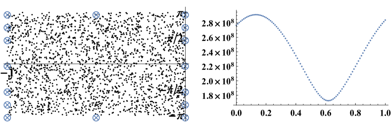
Figure 1. Left: the spectrum of $A$ and the points of interpolation; right: the norms $\lVert\Omega(A)e^{tA}\rVert$ for $t=0.01k$, $k=0,\dots,100$

References

• [1] B. F. Bylov, R. È. Vinograd, D. M. Grobman, and V. V. Nemyckii, The theory of Lyapunov exponents and its applications to problems of stability, Izdat. “Nauka”, Moscow, 1966, (in Russian). MR 0206415
• [2] M. Crouzeix, Bounds for analytical functions of matrices, Integral Equations Operator Theory 48 (2004), no. 4, 461–477. MR 2047592
• [3] Ph. J. Davis, Interpolation and approximation, Dover Publications, Inc., New York, 1975. MR 0380189
• [4] A. Frommer and V. Simoncini, Matrix functions, in Model order reduction: theory, research aspects and applications, W. H. Schilders, H. A. van der Vorst, and J. Rommes, eds., vol. 13 of Mathematics in Industry, Springer, Berlin, 2008, pp. 275–303. MR 2497756
• [5] I. M. Gelfand and G. E. Shilov, Generalized functions. Vol. 3: Theory of differential equations, Academic Press, New York–London, 1967, Translated from the Russian. MR 0217416
• [6] A. O. Gelfond, Calculus of finite differences, second ed., GIFML, Moscow, 1959, (in Russian); translated by Hindustan Publishing Corp., Delhi, in series International Monographs on Advanced Mathematics and Physics, 1971. MR 0342890
• [7] M. I. Gil, Estimate for the norm of matrix-valued functions, Linear and Multilinear Algebra 35 (1993), no. 1, 65–73. MR 1310964
• [8] by same author, Estimates for entries of matrix valued functions of infinite matrices, Math. Phys. Anal. Geom. 11 (2008), no. 2, 175–186. MR 2438734
• [9] by same author, A norm estimate for holomorphic operator functions in an ordered Banach space, Acta Sci. Math. (Szeged) 80 (2014), no. 1-2, 141–148. MR 3236255
• [10] G. H. Golub and Ch. F. Van Loan, Matrix computations, third ed., Johns Hopkins Studies in the Mathematical Sciences, Johns Hopkins University Press, Baltimore, MD, 1996. MR 1417720
• [11] A. Greenbaum, Some theoretical results derived from polynomial numerical hulls of Jordan blocks, Electron. Trans. Numer. Anal. 18 (2004), 81–90. MR 2114450
• [12] N. J. Higham, Functions of matrices: theory and computation, Society for Industrial and Applied Mathematics (SIAM), Philadelphia, PA, 2008. MR 2396439
• [13] E. Hille and R. S. Phillips, Functional analysis and semi-groups, American Mathematical Society Colloquium Publications, vol. 31, Amer. Math. Soc., Providence, Rhode Island, 1957. MR 0089373
• [14] Ch. Jordan, Calculus of finite differences, third ed., Chelsea Publishing Co., New York, 1965. MR 0183987
• [15] Bo Kágström, Bounds and perturbation bounds for the matrix exponential, Nordisk Tidskr. Informationsbehandling (BIT) 17 (1977), no. 1, 39–57. MR 0440896
• [16] R. Mathias, Approximation of matrix-valued functions, SIAM J. Matrix Anal. Appl. 14 (1993), no. 4, 1061–1063. MR 1238920
• [17] Ch. F. Van Loan, A study of the matrix exponential, Numerical Analysis Report No. 10, University of Manchester, Manchester, UK, August 1975, Reissued as MIMS EPrint 2006.397, Manchester Institute for Mathematical Sciences, The University of Manchester, UK, November 2006.
• [18] by same author, The sensitivity of the matrix exponential, SIAM J. Numer. Anal. 14 (1977), no. 6, 971–981. MR 0468137
• [19] N. J. Young, A bound for norms of functions of matrices, Linear Algebra Appl. 37 (1981), 181–186. MR 636219