Online scheduling of jobs with favorite machines

Abstract

This work introduces a natural variant of the online machine scheduling problem on unrelated machines, which we refer to as the favorite machine model. In this model, each job has a minimum processing time on a certain set of machines, called favorite machines, and some longer processing times on other machines. This type of costs (processing times) arise quite naturally in many practical problems. In the online version, jobs arrive one by one and must be allocated irrevocably upon each arrival without knowing the future jobs. We consider online algorithms for allocating jobs in order to minimize the makespan.

We obtain tight bounds on the competitive ratio of the greedy algorithm and characterize the optimal competitive ratio for the favorite machine model. Our bounds generalize the previous results of the greedy algorithm and the optimal algorithm for the unrelated machines and the identical machines. We also study a further restriction of the model, called the symmetric favorite machine model, where the machines are partitioned equally into two groups and each job has one of the groups as favorite machines. We obtain a 2.675-competitive algorithm for this case, and the best possible algorithm for the two machines case.

1 Introduction

Online scheduling on the unrelated machines is a classical and well-studied problem. In this problem, there are $n$ jobs that need to be processed by one of $m$ different machines. The jobs arrive one by one and must be assigned to one machine upon their arrival, without knowing the future jobs. The time to process a job changes from machine to machine, and the goal is to allocate all jobs so as to minimize the makespan, that is, the maximum load over the machines. The load of a machine is the sum of the processing times of the jobs allocated to that machine.

Online algorithms are designed to solve the problems when the input is not known from the very beginning but released “piece-by-piece” as aforementioned. Since it is generally impossible to guarantee an optimal allocation, online algorithms are evaluated through the competitive ratio. An online algorithm whose competitive ratio is $\rho\geq 1$ guarantees an allocation whose makespan is at most $\rho$ times the optimal makespan.

For scheduling on unrelated machines, online algorithms have a rather “bad” performance in terms of the competitive ratio. For example, the simple greedy algorithm has a competitive ratio of $m$, the number of machines; the best possible online algorithm achieves a competitive ratio of $\Theta(\log m)$. However, some well-known restrictions (e.g., the identical machines and related machines) admit a much better performance, that is, a constant competitive ratio.

In fact, many practical problems are neither as simple as the identical (or related) machines cases, nor so complicated as the general unrelated machines. In a sense, practical problems are somewhat “intermediate” as the following examples suggest.

Example 1 (Two types of jobs (Vakhania et al., 2014)).

This restriction of unrelated machines arises naturally when there are two types of products. For instance, consider the production of spare parts for cars. The manufacturer may decide to use the machines for the production of spare part 1 to produce spare part 2, and vice versa. The machine for spare part 1 (spare part 2, respectively) takes time $p$ for part 1 (part 2, respectively), but it can also manage to produce part 2 (part 1, respectively) in time $q>p$.

Example 2 (CPU-GPU cluster (Chen et al., 2014)).

A graphics processing unit (GPU) has the ability to handle various tasks more efficiently than the central processing unit (CPU). These tasks include video processing, image analysis, and signal processing. Nevertheless, the CPU is still more suitable for a wide range of other tasks. A heterogeneous CPU-GPU system consists of a set $M_{1}$ of GPU processors and a set $M_{2}$ of CPU processors. The processing time of job $j$ is $p_{j1}$ on a GPU processor and $p_{j2}$ on a CPU processor. Therefore, some jobs are more suitable for GPU and others for CPU.

Inspired by these examples, we consider the general unrelated machines case by observing that each job in the system has a certain set of favorite machines which correspond to the shortest processing time for this particular job. In Example 1, the machines for spare parts $1$ are the favorite machines for these parts (processing time $p<q$), and similarly for spare parts $2$. In Example 2, we also have two type of machines (GPU and CPU) and some jobs (tasks) have GPUs as favorite machines and others have CPUs as favorite machines.

1.1 Our contributions and connections with prior work

We study the online scheduling problem on what we call the favorite machine model. Denote the processing time of job $j$ on machine $i$ by $p_{{j}{i}}$ and the minimum processing time of job $j$ by $p_{{j}{}}=\min_{i}p_{{j}{i}}$. Thus the set of favorite machines of job $j$ is defined as $F_{j}=\{i|\ p_{{j}{i}}=p_{{j}{}}\}$ and the favorite machine model is as follows:

($f$-favorite machines) This model is simply the unrelated machine setting when every job $j$ has at least $f$ favorite machines ($|F_{j}|\geq f$). The processing time of job $j$ on any favorite machine $i\in F_{j}$ is $p_{{j}{}}$, and on any non-favorite machine $i\notin F_{j}$ is an arbitrary value $p_{{j}{i}}>p_{{j}{}}$.

This model is motivated by several practical scheduling problems. Besides the two types of jobs/machines problems mentioned in Examples 1 and 2, the model also captures the features of some real life problems. For example, workers with different levels of proficiency for different jobs in manufacturing; tasks/data transfer cost in cloud computing and so on.

It is worth noting that this model interpolates between the unrelated machines where possibly only one machine has minimal processing time for the job ($f=1$) and the identical machines case $(f=m)$. The $f$-favorite machines setting can also be seen as a “relaxed” version of restricted assignment problem where each job $j$ can be allocated only to a subset $F_{j}$ of machines: the restricted assignment problem is essentially the case where the processing time of a job on a non-favorite machine is always $\infty$.

We obtain tight bounds on the Greedy algorithm and the well-known Assign-U algorithm (designed for unrelated machines by Aspnes et al. (1997)) for the $f$-favorite machines case, and show the optimality of the Assign-U algorithm by providing a matching lower bound. For the Greedy algorithm, the competitive ratio is $\frac{m+f-1}{f}$, which generalizes the well-known bounds on the competitive ratio of Greedy for unrelated machines ($f=1$) and identical machines ($f=m$), that is, $m$ and $2-\frac{1}{m}$, respectively. The Assign-U algorithm has the optimal competitive ratio $\Theta(\log\frac{m}{f})$, while it is $\Theta(\log{m})$ for unrelated machines.

Easier instances and the impact of “speed ratio”.

Note that whenever $f=\Theta(m)$, the competitive ratio is constant. In particular, for $f=\frac{m}{2}$, Greedy has a competitive ratio of $3-\frac{2}{m}$. We consider the following restriction of the model above such that a finer analysis is possible.

(symmetric $\frac{m}{2}$-favorite machines) All machines are partitioned into two groups of equal size $\frac{m}{2}$, and each job has favorite machines as exactly one of the two groups (therefore $f=\frac{m}{2}$ and $m$ is even). Moreover, the processing time on non-favorite machines is $s$ times that on favorite machines, where $s\geq 1$ is the scaling factor (the “speed ratio” between favorite and non-favorite machines).

We show that the competitive ratio of Greedy is at most $\min\{1+(2-\frac{2}{m})\frac{s^{2}}{s+1},~{}s+(2-\frac{2}{m})\frac{s}{s+1},~{}3-\frac{2}{m}\}~{}(<3)$. A modified greedy algorithm, called GreedyFavorite, which assigns each job greedily but only among its favorite machines, has a competitive ratio of $2-\frac{1}{f}+\frac{1}{s}~{}(<3)$. As one can see, the Greedy is better than GreedyFavorite for smaller $s$, and GreedyFavorite is better for larger $s$. Thus we can combine the two algorithms to obtain a better algorithm (GGF) with a competitive ratio of at most $\min\{2+\frac{s^{2}+s-2}{s+1},2+\frac{1}{s}\}~{}(\leq 2.675)$. Indeed, we characterize the optimal competitive ratio for the two machines case. That is, for symmetric $1$-favorite machines, we show that the GGF algorithm is $\min\{1+\frac{s^{2}}{s+1},1+\frac{1}{s}\}$-competitive and there is a matching lower bound.

For this problem, our results show the impact of the speed ratio $s$ on the competitive ratio. This is interesting because this problem generalizes the case of two related machines (Epstein et al., 2001), for which $s$ is the speed ratio between the two machines. The two machines case has also been studied earlier from a game theoretic point of view and compared to the two related machines (Chen et al., 2017; Epstein, 2010).

Figure 1: Comparison between prior problems and results (in red) and our problems and results (in blue). The two bounds below each problem are the competitive ratios for Greedy and best-known algorithm, respectively, and the “${(*)}$” mark represent the optimality of the best-known algorithm. Arrows go from a problem to a more general one, and therefore the upper bounds for the general problem apply to the special one as well.

Relations with prior work.

As mentioned above, the $f$-favorite machines is a special case of the unrelated machines and a general case of the identical machines. The symmetric 1-favorite machines is a generalization of the 2 related machines.

Besides, there are several other “intermediate” problems that have connections with our models and results in the literature (see Figure 1 for an overview). Specifically, in the two types of machines case (Imreh, 2003; Chen et al., 2014), they have two sets of machines, $M_{1}$ and $M_{2}$, and the machines in each set are identical. Each job $j$ has processing time $p_{j1}$ for any machine in $M_{1}$, and $p_{j2}$ for any machine in $M_{2}$. The so-called balanced case is the restriction in which the number of machines in the two sets are equal. Note that our $\frac{m}{2}$-favorite machines is a generalization of the balanced case, because each job has either $M_{1}$ or $M_{2}$ as favorite machines, and thus $f=|M_{1}|=|M_{2}|=\frac{m}{2}$. The symmetric $\frac{m}{2}$-favorite machines case is the restriction of the balance case in which the processing time on non-favorite machines is $s$ times that of favorite ones, i.e., either $p_{j1}=s\cdot p_{j2}$ or $p_{j2}=s\cdot p_{j1}$.

1.2 Related work

The Greedy algorithm (also known as List algorithm) is a natural and simple algorithm, often with a provable good performance. Because of its simplicity, it is widely used in many scheduling problems. In some cases, however, better algorithms exist and Greedy is not optimal.

Identical machines. For $m$ identical machines, the Greedy algorithm has a competitive ratio exactly $2-1/m$ (Graham, 1966), and this is optimal for $m=2,3$ (Faigle et al., 1989). For arbitrary larger $m$, better online algorithms exist and the bound is still improving (Karger et al., 1996; Bartal et al., 1995; Albers, 1999). Till now the best-known upper bound is 1.9201 (Fleischer and Wahl, 2000) and the lower bound is 1.88 (Rudin III, 2001).

Related machines (uniform processors). The competitive ratio of Greedy is ${(1+\sqrt{5})}/{2}\approx 1.618$ for two machines ($m=2$), and it is at most $1+\sqrt{2m-2}/2$ for $m\geq 3$. The bounds are tight for $m\leq 6$ (Cho and Sahni, 1980).

When the number of machines $m$ becomes larger, the Greedy algorithm is far from optimal, as its competitive ratio is $\Theta(\log m)$ for arbitrary $m$ (Aspnes et al., 1997). Aspnes et al. (1997) also devise the Assign-R algorithm with the first constant competitive ratio of 8 for related machines. The constant is improved to 5.828 by Berman et al. (2000).

Some research focuses on the dependence of the competitive ratio on speed $s$ when $m$ is rather small. For the 2 related machines case, Greedy has a competitive ratio of $1+\min\{\frac{s}{s+1},\frac{1}{s}\}$ and there is a matching lower bound (Epstein et al., 2001).

Unrelated machines. As to the unrelated machines, Aspnes et al. (1997) show that the competitive ratio of Greedy is rather large, namely $m$. In the same work, they present the algorithm Assign-U with a competitive ratio of $\mathcal{O}(\log m)$. A matching lower bound is given by Azar et al. (1992) in the problem of online restricted assignment.

Restricted assignment. The online restricted assignment problem is also known as online scheduling subject to arbitrary machine eligibility constraints. Azar et al. (1992) show that Greedy has a competitive ratio less than $\lceil\log_{2}m\rceil+1$, and there is a matching lower bound $\lceil\log_{2}(m+1)\rceil$. For other results of online scheduling with machine eligibility we refer the reader to the survey by Lee et al. (2013) and references therein.

Two types of machines (CPU-GPU cluster, hybrid systems). Imreh (2003) proves that Greedy algorithm is $(2+\frac{m_{1}-1}{m_{2}})$-competitive for this case, where $m_{1}$ and $m_{2}$ ($\leq m_{1}$) are the number of two sets of machines, respectively. In our terminology, $f=m_{2}$ and $m_{1}=m-f$, meaning that Greedy is $(1+\frac{m-1}{f})$-competitive for $f\leq\frac{m}{2}$. The same work also improves the bound to $4-\frac{2}{m_{1}}$ with a modified Greedy algorithm. Chen et al. (2014) gives a $3.85$-competitive algorithm for the problem, and a simple $3$-competitive algorithm and a more involved $1+\sqrt{3}\approx 2.732$-competitive algorithm for the balanced case, that is, the case $m_{1}=m_{2}$.

Further models and results. Some work consider restrictions on the processing times in the offline version of scheduling problems. Specifically, Vakhania et al. (2014) consider the case of two processing times, where each processing time $p_{ji}\in\{q,p\}$ for all $i$ and $j$. Kedad-Sidhoum et al. (2018) consider the two types of machines (CPU-GPU cluster) problem, and Gehrke et al. (2018) consider a generalization, the few types of machines problem. Some work also study similar models in a game-theoretic setting (Lavi and Swamy, 2009; Auletta et al., 2015). Regarding online algorithms, several works consider restricted assignment with additional assumptions on the problem structure like hierarchical server topologies (Bar-Noy et al., 2001) (see also Crescenzi et al. (2007)). For other results of processing time restrictions, we refer the reader to the survey by Leung and Li (2008). Finally, the $f$-favorite machine model in our paper has been recently analyzed in a follow-up paper in the offline game-theoretic setting (Chen and Xu, 2018).

2 Model and preliminary definitions

The favorite machines setting.

There are $m$ machines, $\mathcal{M}:=\{1,2,\dots,m\}$, to process $n$ jobs, $\mathcal{J}:=\{1,2,\dots,n\}$. Denote the processing time of job $j$ on machine $i$ by $p_{{j}{i}}$, and the minimum processing time of job $j$ by $p_{{j}{}}=\min_{i\in\mathcal{M}}p_{{j}{i}}$. We define the favorite machines of a job as the machines with the minimum processing time for the job. Let $F_{j}\subseteq\mathcal{M}$ be the set of favorite machines of job $j$. Assume that each job has at least $f$ favorite machines, i.e., $|F_{j}|\geq f$ for $j\in\mathcal{J}{}$. Thus, the processing time of job $j$ on its favorite machines equals to the minimum processing time $p_{{j}{}}$ (i.e., $p_{{j}{i}}=p_{{j}{}}$ for $i\in F_{j}$), while the processing time on its non-favorite machines can be any value that greater than $p_{{j}{}}$ (i.e., $p_{{j}{i}}>p_{{j}{}}$ for $i\notin F_{j}$).

The symmetric favorite machines setting.

This setting is the following restriction of the favorite machines. There are $m=2f$ machines partitioned into two subsets of $f$ machines each, that is, $\mathcal{M}{}=M_{1}\cup M_{2}$, where $M_{1}=\{1,2,\dots,f\}$ and $M_{2}=\{f+1,f+2,\dots,2f\}$. Each job $j$ has either $M_{1}$ or $M_{2}$ as its favorite machines, i.e., $F_{j}\in\{M_{1},M_{2}\}$. The processing time of job $j$ is $p_{{j}{}}$ on its favorite machines and $s\cdot p_{{j}{}}$ on non-favorite machines, where $s\geq 1$.

Further notation.

We say that job $j$ is a good job if it is allocated to one of its favorite machines, and it is a bad job otherwise.

Let $l_{i}{(j)}$ denote the load on machine $i$ after jobs $1$ through $j$ are allocated by online algorithm:

$$l_{i}{(j)}=\begin{cases}l_{i}{(j-1)}+p_{{j}{i}}\,,&\text{if job $j$ is assigned to machine $i$}\,,\\ l_{i}{(j-1)}\,,&\text{otherwise.}\end{cases}$$

In the analysis, we shall sometimes considered the machines in non-increasing order of their loads. For a sequence jobs, we denote by $\ell_{i}{(j)}$ the $i^{th}$ highest load over all machines after the first $j$ jobs are allocated, i.e.,

$$\ell_{1}{(j)}\geq\ell_{2}{(j)}\geq\cdots\geq\ell_{m}{(j)}\,,\quad\text{for any $j\in\mathcal{J}$}.$$

The jobs arrive one by one (over a list) and must be allocated irrevocably upon each arrival without knowing the future jobs. the goal is to minimize the makespan, the maximum load over all machines. The competitive ratio of an algorithm $A$ is defined as $\rho_{A}:=\sup_{I}\frac{C_{A}(I)}{C_{\textsc{opt}}(I)},$ where $I$ is taken over all possible sequences of jobs, $C_{A}(I)$ is the cost (makespan) of algorithm $A$ on sequence $I$, and $C_{\textsc{opt}}(I)$ is the optimal cost on the same sequence. We write $C_{A}$ and $C_{\textsc{opt}}$ for simplicity whenever the job sequence is clear from the context.

3 The favorite machine model

In this section, we first analyze the performance of the Greedy algorithm and show its competitive ratio is precisely $\frac{m+f-1}{f}$. We then show that no online algorithm can be better than $\Omega(\log\frac{m}{f})$ and that algorithm Assign-U (Aspnes et al., 1997) has an optimal competitive ratio of $\mathcal{O}(\log\frac{m}{f})$ for our problem.

3.1 Greedy Algorithm

Algorithm Greedy: Every job is assigned to a machine that minimizes the completion time of this job (the completion time of job $j$ if allocated to machine $i$ is the load $l_{i}{(j)}$ of machine $i$ after the job is allocated).

Theorem 3.

The competitive ratio of Greedy is at most $\frac{m+f-1}{f}$.

The key part in the proof of Theorem 3 is the following lemma which says that Greedy maintains the following invariant: the sum of the $f$ largest machines loads never exceeds the sum of all jobs’ minimal processing times.

Lemma 4.

For $f$-favorite machines, and for every sequence of $n$ jobs, the allocation of Greedy satisfies the following condition:

$$\ell_{1}{(n)}+\ell_{2}{(n)}+\cdots+\ell_{f}{(n)}\leq p_{{1}{}}+p_{{2}{}}+\cdots+p_{{n}{}}\,.$$ (1)

Proof.

The proof is by induction on the number $n$ of jobs released so far. The base case is $n=1$. Since Greedy allocates the first job to one of its favorite machines, and the other machines are empty, we have $\sum_{i=1}^{f}\ell_{i}{(1)}=\ell_{i}{(1)}=p_{{1}{}}$, and thus (1) holds for $n=1$.

As for the inductive step, we assume that (1) holds for $n-1$, i.e.,

$$\ell_{1}{(n-1)}+\ell_{2}{(n-1)}+\cdots+\ell_{f}{(n-1)}\leq p_{{1}{}}+p_{{2}{}}+\cdots+p_{{n-1}{}}\,,$$ (2)

and show that the same condition holds for $n$, i.e., after job $n$ is allocated.

If job $n$ is allocated as a good job, then the left-hand side of (2) will increase by at most $p_{{n}{}}$, while the right-hand side will increase by exactly $p_{{n}{}}$. Thus, equation (1) follows from the inductive hypothesis (2).

If job $n$ is allocated as a bad job on some machine $b$, then the following observation allows to prove the statement: before job $n$ is allocated, the load of each favorite machine for job $n$ must be higher than $l_{b}{(n-1)}$ (otherwise Greedy would allocate $n$ as a good job). Since there are at least $f$ favorite machines for job $n$, there must be a favorite machine $a$ with

$$l_{b}{(n-1)}<l_{a}{(n-1)}\leq\ell_{f}{(n-1)}\ .$$ (3)

Thus, $l_{b}{(n-1)}$ is not one of the $f$ largest loads before job $n$ is allocated. After allocating job $n$, the load of machine $b$ increases to $l_{b}{(n)}=l_{b}{(n-1)}+p_{{n}{b}}$. We then have two cases depending on whether $l_{b}{(n)}$ is one of the $f$ largest loads after job $n$ is allocated:

Case 1 ($l_{b}{(n)}\leq\ell_{f}{(n-1)}$). In this case, the $f$ largest loads remain the same after job $n$ is allocated, meaning that the left-hand side of (2) does not change, while the right-hand side increases (when adding job $n$). In other words, (1) follows from the inductive hypothesis (2).

Case 2 ($l_{b}{(n)}>\ell_{f}{(n-1)}$). In this case, $\ell_{f}{(n-1)}$ will be no longer included in the first $f$ largest loads, after job $n$ is allocated, while $l_{b}{(n)}$ will enter the set of $f$ largest loads:

$$\sum_{~{}\>i=1~{}\>}^{f}\ell_{i}{(n)}=\sum_{~{}\>i=1~{}\>}^{f}\ell_{i}{(n-1)}-\ell_{f}{(n-1)}+l_{b}{(n)}\,.$$ (4)

Since Greedy allocates job $n$ to machine $b$, it must be the case

$$l_{b}{(n)}=l_{b}{(n-1)}+p_{{n}{b}}\leq l_{a}{(n-1)}+p_{{n}{}}\leq\ell_{f}{(n-1)}+p_{{n}{}}\,,$$ (5)

where $a$ is the favorite machine satisfying (3). Substituting (5) into (4) and by inductive hypothesis (2), we obtain $\sum_{i=1}^{f}\ell_{i}{(n)}\leq\sum_{i=1}^{f}\ell_{i}{(n-1)}+p_{{n}{}}\leq\sum_{i=1}^{n-1}p_{{i}{}}+p_{{n}{}}$, and thus (1) holds. This completes the proof of the lemma. ∎

Proof of Theorem 3.

Without loss of generality we, assume that the makespan of the allocation of Greedy is determined by the last job $n$ (otherwise, we can consider the last job $n^{\prime}$ which determines the makespan, and ignore all jobs after $n^{\prime}$ since they do not increase $C_{\textsc{Greedy}}$ nor decrease $C_{\textsc{opt}}$).

After allocating the last job $n$, the cost of Greedy becomes

$$C_{\textsc{Greedy}}{} \leq\min\left\{\min_{i\in F_{n}}l_{i}{(n-1)}+p_{{n}{}},\,\min_{i\in\mathcal{M}{}\backslash F_{n}}l_{i}{(n-1)}+p_{{n}{i}}\right\}$$

$$\leq\min_{i\in F_{n}}l_{i}{(n-1)}+p_{{n}{}}$$

$$\leq\ell_{f}{(n-1)}+p_{{n}{}}\,,$$ (6)

where the last inequality holds because job $n$ has at least $f$ favorite machines, and thus the least loaded among them must have load at most $\ell_{f}{(n-1)}$.

Since the optimum must allocate all jobs on $m$ machines, and job $n$ itself requires $p_{{n}{}}$ on a single machine, we have

$$C_{\textsc{opt}}{}\geq\max\left\{\frac{\sum_{j=1}^{n}p_{{j}{}}}{m},\,p_{{n}{}}\right\}\geq\max\left\{\frac{f\cdot\ell_{f}{(n-1)}+p_{{n}{}}}{m},\,p_{{n}{}}\right\}\,.$$ (7)

where the second inequality is due to Lemma 4 applied to the first $n-1$ jobs only (specifically, we have $\sum_{j=1}^{n-1}p_{{j}{}}\geq\sum_{i=1}^{f}\ell_{i}{(n-1)}\geq f\cdot\ell_{f}{(n-1)}$). By combining (3.1) and (7), we obtain

$$\frac{C_{\textsc{Greedy}}{}}{C_{\textsc{opt}}{}} \leq\frac{\ell_{f}{(n-1)}+p_{{n}{}}}{\max\left\{\frac{f\cdot\ell_{f}{(n-1)}+p_{{n}{}}}{m},\,p_{{n}{}}\right\}}$$

$$=\min\left\{\frac{m\left(\frac{\ell_{f}{(n-1)}}{p_{{n}{}}}+1\right)}{f\frac{\ell_{f}{(n-1)}}{p_{{n}{}}}+1},\,\frac{\ell_{f}{(n-1)}}{p_{{n}{}}}+1\right\}$$

$$\leq\frac{m+f-1}{f}\,,$$

where the last inequality holds because the first term decreases in ${\ell_{f}{(n-1)}}/{p_{{n}{}}}$ and the second term increases in ${\ell_{f}{(n-1)}}/{p_{{n}{}}}$. ∎

Theorem 5.

The competitive ratio of Greedy is at least $\frac{m+f-1}{f}$.

Proof.

We will provide a sequence of jobs whose schedule by Greedy has a makespan $\frac{m+f-1}{f}$, and the optimal makespan is 1. For simplicity, we assume that in case of a tie, the Greedy algorithm will allocate the job as a bad job to a machine with the smallest index. Without loss of generality, suppose $m$ is divisible by $f$. We partition the $m$ machines into $m^{\prime}:=\frac{m}{f}$ groups, $M_{1},M_{2},\dots,M_{m^{\prime}}$, each of them containing $f$ machines, i.e., $M_{i}=\{(i-1)f+1,\,(i-1)f+2,\dots,\,(i-1)f+f\}$ for $i=1,\dots,m^{\prime}$.

The jobs are released in two phases (described in detail below): In the first phase, we force Greedy to allocate each machine in $M_{i}$ a load of bad jobs equal to $i-1$, and a load of good jobs equal to $1-\frac{i}{s}$ for a suitable $s>1$ (except for $M_{m^{\prime}}$); In the second phase, several jobs with favorite machines in $M_{m^{\prime}}$ are released and contribute an additional $2-\frac{1}{f}$ to the load of one machine in $M_{m^{\prime}}$, and thus the makespan is $\frac{m+f-1}{f}$.

We use the notation $r\times(p,F)$ to represent a sequence of $r$ identical jobs whose favorite machines are $F$, the processing time on favorite machines is $p$, and on non-favorite machines is $s\cdot p$ with $s\geq 1$.

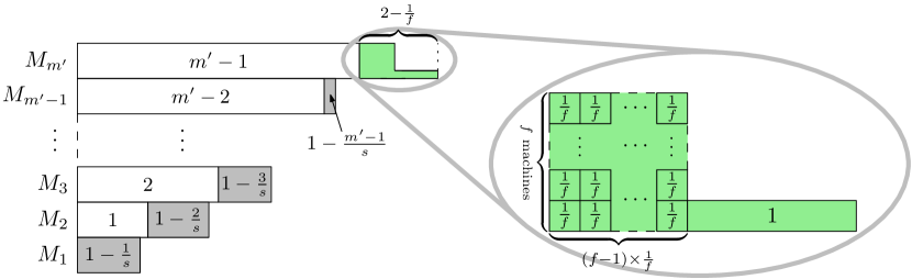
Figure 2: Proof of Theorem 5 (bad jobs in white).

Phase 1. For each $i$ from $1$ to $m^{\prime}-1$, release a sequence of jobs $f\times(1-\frac{i}{s},M_{i})$ followed by a sequence $f\times(\frac{i}{s},M_{i})$. In this phase, we take $s>m^{\prime}-1+\sqrt{(m^{\prime}-1)(m^{\prime}-2)}$, so that, for each $i$, the jobs $f\times(1-\frac{i}{s},M_{i})$ will be assigned as good jobs to the $f$ machines in $M_{i}$, one per machine, and the jobs $f\times(\frac{i}{s},M_{i})$ will be assigned as bad jobs to the $f$ machines in $M_{i+1}$, one per machine (as shown in Figure 2).

At the end of Phase 1, each machine in $M_{i}$ ($i\in[1,m^{\prime}-1]$) will have load $\frac{i-1}{s}\cdot s+1-\frac{i}{s}=i(1-\frac{1}{s})$, and each machine in $M_{m^{\prime}}$ will have load $m^{\prime}-1$. The optimal schedule assigns every job to some favorite machine evenly so that all machines have load $1$, except for the machines in the last group $M_{m^{\prime}}$ which are left empty.

Phase 2. In this phase, all jobs released have $M_{m^{\prime}}$ as their favorite machines, specifically $f(f-1)\times(\frac{1}{f},M_{m^{\prime}})$ followed by a single job $(1,M_{m^{\prime}})$. By taking $s>m$, no jobs will be allocated as bad jobs by Greedy. Thus, this phase can be seen as scheduling on $f$ identical machines. Consequently, all jobs will be allocated as in Figure 2 increasing the maximum load of machines in $M_{m^{\prime}}$ by $2-\frac{1}{f}$, while the optimal schedule can have a makespan 1.

At the end of Phase 2, the maximum load of machines in $M_{m^{\prime}}$ is $m^{\prime}-1+2-\frac{1}{f}=\frac{m+f-1}{f}$, while the optimal makespan is 1. ∎

3.2 A general lower bound

In this section, we provide a general lower bound for the $f$-favorite machines problem. The bound borrows the basic idea of the lower bound for the restricted assignment (Azar et al., 1992). The trick of our proof is that we always partition the selected machines into arbitrary groups of $f$ machines each, and apply the idea to each of the group respectively.

Theorem 6.

Every deterministic online algorithm must have a competitive ratio at least $\frac{1}{2}\lfloor\log_{2}\frac{m}{f}\rfloor+1$.

Proof.

Suppose first that $\frac{m}{f}$ is a power of 2, i.e., $\frac{m}{f}=2^{{u}-1}$. We provide a sequence of $m$ jobs having optimal makespan equal to $1$, while any online algorithm will have a makespan at least $\frac{u+1}{2}=\frac{1}{2}\log_{2}\frac{m}{f}+1$.

We denote by $r\times(1,F)$ a sequence of $r$ identical jobs whose favorite machines are $F$, the processing time on favorite machines is $1$, and the processing time on non-favorite machines is greater than $\frac{u+1}{2}=\frac{1}{2}\log_{2}\frac{m}{f}+1$, so that all jobs must be allocated to favorite machines.

We consider subsets of machines $\mathcal{M}{}_{1},\mathcal{M}{}_{2},\ldots,\mathcal{M}{}_{u}$, where the first subset is $\mathcal{M}{}_{1}=\mathcal{M}$ and the others satisfy $\mathcal{M}{}_{i}\subset\mathcal{M}{}_{i-1}$ and $|\mathcal{M}{}_{i}|=\frac{1}{2}|\mathcal{M}{}_{i-1}|=\frac{m}{2^{i-1}}$ for $i=2,\ldots u$. We then release $u$ sets of jobs iteratively. At each iteration $i$ ($i=1,2,\ldots,u$), a set of jobs $\mathcal{J}{}_{i}$ with favorite machines $\mathcal{M}{}_{u}$ are released for allocation, and after the allocation, half of the “highly loaded” machines in $\mathcal{M}{}_{i}$ are chosen for the next set $\mathcal{M}{}_{i+1}$. More in detail, for each iteration $i$ ($i=1,2,\ldots,u$) we proceed as follows:

• Partition the current set $\mathcal{M}{}_{i}$ of machines into arbitrary groups of $f$ machines each, that is, into groups $M_{i,1},M_{i,2},\dots,M_{i,m_{i}^{\prime}}$ where $m_{i}^{\prime}=\frac{|\mathcal{M}{}_{i}|}{f}=\frac{m}{f\cdot 2^{i-1}}=2^{{u}-i}$. Then, release a set of jobs $\mathcal{J}{}_{i}$:

  $$\mathcal{J}{}_{i}:=\begin{cases}J_{i,1}\cup J_{i,2}\cup\ldots\cup J_{i,m_{i}^{\prime}}\,,&\text{ if }1\leq i\leq{u}-1\,;\\ \{f\times(1,\mathcal{M}{}_{u})\}\,,&\text{ if }i={u}\,;\end{cases}$$

  where $J_{i,l}:=\left\{\frac{f}{2}\times(1,M_{i,l})\right\}$.

• The next set $\mathcal{M}{}_{i+1}$ of machines consists of the $f/2$ most loaded machines in each subgroup after jobs $\mathcal{J}{}_{i}$ have been allocated. Specifically, we let $\mathcal{M}_{i+1}:=M^{\prime}_{i,1}\cup M^{\prime}_{i,2}\cup\cdots\cup M^{\prime}_{i,m_{i}^{\prime}}$, for $M^{\prime}_{i,l}\subset M{}_{i,l}$ being the subset of $f/2$ most loaded machines in group $M_{i,l}$ after jobs $\mathcal{J}{}_{i}$ have been allocated.

We then show that the following invariant holds at every iteration. Note that the following lemma shows a separation of our method and the one of Azar et al. (1992). Specifically, the maximum load increases by $1/2$ at each iteration in our lower bound, but increases by $1$ in Azar et al. (1992).

Lemma 7.

The average load of machines in $\mathcal{M}{}_{i}$ is at least $\frac{i-1}{2}$ before the jobs in $\mathcal{J}{}_{i}$ are assigned for $1\leq i\leq{u}$.

Proof.

The proof is done by induction on $i$. For the base case $i=1$, the lemma is trivial. As for the inductive step, suppose the lemma holds for $i$.

Denote the average load of $M_{i,l}$ before the allocation of jobs $\mathcal{J}{}_{i}$ by $Avg(i,l)$, and the average load of $M^{\prime}_{i,j}$ after the allocation of jobs $\mathcal{J}{}_{i}$ by $Avg^{\prime}(i,l)$. We claim that $Avg^{\prime}(i,l)\geq Avg(i,l)+1/2$ after the allocation of jobs $\mathcal{J}{}_{i}$. Note that $\mathcal{M}{}_{i}$ and $\mathcal{M}{}_{i+1}$ are the union of all groups $M_{i,l}$ and $M_{i,l}^{\prime}$, respectively. Thus, we have that the average load of $\mathcal{M}{}_{i+1}$ is at least $\frac{i-1}{2}+\frac{1}{2}=\frac{i}{2}$, since the average load of $\mathcal{M}{}_{i}$ is $\frac{i-1}{2}$ (the inductive hypothesis). This concludes the proof of the inductive step, and thus the lemma follows. Next, we prove that the claim $Avg^{\prime}(i,l)\geq Avg(i,l)+1/2$ holds:

Case 1. There is a machine in $M_{i,l}\backslash M^{\prime}_{i,l}$ that has load at least $Avg(i,l)+1/2$. Since $M^{\prime}_{i,l}$ consists of the $f/2$ most loaded machines in $M_{i,l}$, each machine in $M^{\prime}_{i,l}$ will also have load at least $Avg(i,l)+1/2$. Thus, we obtain that $Avg^{\prime}(i,l)\geq Avg(i,l)+1/2$.

Case 2. Each machine in $M_{i,l}\backslash M^{\prime}_{i,l}$ has load no greater than $Avg(i,l)+1/2$. Observe that the total load of $M_{i,l}$ is $k\cdot Ave(i,l)+k/2$ after the allocation of $\mathcal{J}{}_{i}$. Since $M_{i,l}\backslash M^{\prime}_{i,l}$ has load at most $k/2\cdot(Avg(i,l)+1/2)$, the average load of the $f/2$ machines in $M^{\prime}_{i,l}$ must be at least

$$Avg^{\prime}(i,l)\geq\frac{k\cdot Avg(i,l)+\frac{k}{2}-\frac{k}{2}(Avg(i,l)+\frac{1}{2})}{k/2}=Avg(i,l)+\frac{1}{2}\,.\qed$$

By applying Lemma 7 with $i=u$, we have that the average load of $\mathcal{M}{}_{u}$ is at least $\frac{{u}-1}{2}$ before the allocation of jobs $\mathcal{J}{}_{u}$. Thus, after jobs in $\mathcal{J}{}_{u}$ are allocated, the average load of $\mathcal{M}{}_{u}$ is at least $\frac{{u}-1}{2}+1=\frac{{u}+1}{2}$, i.e., the online cost is at least $\frac{{u}+1}{2}$.

An optimal cost of $1$ can be achieved by using the machines in $M_{i,l}\backslash M^{\prime}_{i,l}$ for $\mathcal{J}{}_{i}$ (for $1\leq i\leq{u}-1$ and $1\leq l\leq m_{i}^{\prime}$) and using machines in $\mathcal{M}{}_{u}$ for $\mathcal{J}{}_{u}$. Therefore, the competitive ratio is at least $\frac{{u}+1}{2}=\frac{1}{2}\log_{2}\frac{m}{f}+1$. Finally, if $\frac{m}{f}$ is not a power of $2$, we simply apply the previous construction to a subset of $m^{*}$ machines, for $\frac{m^{*}}{f}=2^{\lfloor u\rfloor-1}$ and $u=1+\log_{2}\frac{m}{f}$. This gives the desired lower bound $\frac{\lfloor u\rfloor+1}{2}=\frac{1}{2}\lfloor\log_{2}\frac{m}{f}\rfloor+1$. ∎

3.3 General upper bound (Algorithm Assign-U is optimal)

In this section, we prove a matching upper bound for $f$-favorite machines. Specifically, we show that the optimal online algorithm for unrelated machines (algorithm Assign-U by Aspnes et al. (1997) described below) yields an optimal upper bound:

Theorem 8.

Algorithm Assign-U can be used to achieve $\mathcal{O}(\log\frac{m}{f})$ competitive ratio.

Following Aspnes et al. (1997), we show that the algorithm has an optimal competitive ratio $\rho$ (Lemma 9) for the case the optimal cost $C_{\textsc{opt}}{}(\mathcal{J}{})$ is known, and then apply a standard doubling approach to get an algorithm with competitive ratio $4\rho$ for the case the optimum is not known in advance (Theorem 8). In the following, we use a “tilde” notation to denote a normalization by the optimal cost $C_{\textsc{opt}}{}(\mathcal{J}{})$, i.e., $\tilde{x}=x/C_{\textsc{opt}}{}(\mathcal{J}{})$.

Algorithm Assign-U (Aspnes et al., 1997): Each job $j$ is assigned to machine $i^{*}$, where $i^{*}$ is the index minimizing $\Delta_{i}=a^{\tilde{l}_{i}{(j-1)}+\tilde{p}_{{j}{i}}}-a^{\tilde{l}_{i}{(j-1)}}$, where $a>1$ is a suitable constant.

Lemma 9.

If the optimal cost is known, Assign-U has a competitive ratio of $\mathcal{O}(\log\frac{m}{f})$.

Proof.

Without loss of generality, we assume that the makespan of the allocation of Assign-U is determined by the last job $n$ (this is the same as the proof of Theorem 3 above). Let $l^{*}_{i}{(j)}$ be the load of machine $i$ in the optimal schedule after the first $j$ jobs are assigned. Define the potential function:

$$\Phi(j)=\sum_{i=1}^{m}a^{\tilde{l}_{i}{(j)}}\left(\gamma-\tilde{l}^{*}_{i}{(j)}\right)\,,$$ (8)

where $a,\gamma>1$ are constants. Similarly to the proof in Aspnes et al. (1997), we have that the potential function (8) is non-increasing for $a=1+1/\gamma$ (see Appendix A.1 for details). Since $\Phi(0)\geq\Phi(n-1)$ and $\tilde{l}^{*}_{i}{(n-1)}\leq 1$, we have

$$\gamma\cdot m\geq\sum_{i=1}^{m}a^{\tilde{l}_{i}{(n-1)}}\left(\gamma-\tilde{l}^{*}_{i}{(n-1)}\right)\geq\sum_{i=1}^{m}a^{\tilde{l}_{i}{(n-1)}}(\gamma-1)\geq f\cdot a^{\tilde{\ell}_{f}{(n-1)}}(\gamma-1)\,.$$

Thus, it follows that

$$\ell_{f}{(n-1)}\leq\log_{a}\left(\frac{\gamma}{\gamma-1}\cdot\frac{m}{f}\right)\cdot C_{\textsc{opt}}{}\,.$$ (9)

Claim 10.

$C_{\textsc{Assign-U}}{}\leq\ell_{f}{(n-1)}+p_{{n}{}}$ .

Proof.

Suppose Assign-U assigns the last job $n$ to machine $i^{\prime}$, it holds that

$$C_{\textsc{Assign-U}}{}=l_{i^{\prime}}{(n-1)}+p_{{n}{i^{\prime}}}\,,$$

since we suppose job $n$ is the last completed job.

Case 1. Job $n$ is allocated as a good job, i.e., $p_{{n}{i^{\prime}}}=p_{{n}{}}$. According to the rule of Assign-U, machine $i^{\prime}$ must be one of the machines in $F_{n}$ that has the minimum load. Since there are at least $f$ favorite machines, it holds that $l_{i^{\prime}}{(n-1)}\leq\ell_{f}{(n-1)}$. Thus, $C_{\textsc{Assign-U}}{}\leq\ell_{f}{(n-1)}+p_{{n}{}}$.

Case 2. Job $n$ is allocated as a bad job, i.e., $p_{{n}{i^{\prime}}}>p_{{n}{}}$. Let $i^{\prime\prime}$ be the machine who has the minimum load in $F_{n}$. Note that $l_{i^{\prime\prime}}{(n-1)}\leq\ell_{f}{(n-1)}$. According to the rule of Assign-U, it holds that $l_{i^{\prime}}{(n-1)}\leq l_{i^{\prime\prime}}{(n-1)}$; otherwise, we have $\Delta_{i^{\prime}}\geq\Delta_{i^{\prime\prime}}$, which is contradictory to that Assign-U assigns job $n$ to machine $i^{\prime}$.

Since $\Delta_{i^{\prime}}\leq\Delta_{i^{\prime\prime}}$ and $l_{i^{\prime}}{(n-1)}\leq l_{i^{\prime\prime}}{(n-1)}\leq\ell_{f}{(n-1)}$, we have

$$a^{\frac{l_{i^{\prime}}{(n-1)}+p_{{n}{i^{\prime}}}}{C_{\textsc{opt}}{}}}-a^{\frac{l_{i^{\prime}}{(n-1)}}{C_{\textsc{opt}}{}}}\leq a^{\frac{l_{i^{\prime\prime}}{(n-1)}+p_{{n}{i^{\prime\prime}}}}{C_{\textsc{opt}}{}}}-a^{\frac{l_{i^{\prime\prime}}{(n-1)}}{C_{\textsc{opt}}{}}}\,,$$

so that ${\frac{l_{i^{\prime}}{(n-1)}+p_{{n}{i^{\prime}}}}{C_{\textsc{opt}}{}}}\leq{\frac{l_{i^{\prime\prime}}{(n-1)}+p_{{n}{i^{\prime\prime}}}}{C_{\textsc{opt}}{}}}\leq{\frac{\ell_{f}{(n-1)}+p_{{n}{i^{\prime\prime}}}}{C_{\textsc{opt}}{}}}\,,$ implying

$$C_{\textsc{Assign-U}}{}=l_{i^{\prime}}{(n-1)}+p_{{n}{i^{\prime}}}\leq\ell_{f}{(n-1)}+p_{{n}{i^{\prime\prime}}}=\ell_{f}{(n-1)}+p_{{n}{}}\,.\qed$$

According to Claim 10 and (9), we have

$$\frac{C_{\textsc{Assign-U}}{}}{C_{\textsc{opt}}{}} \leq\frac{\ell_{f}{(n-1)}+p_{{n}{}}}{C_{\textsc{opt}}{}}\leq\log_{a}\Big{(}\frac{\gamma}{\gamma-1}\cdot\frac{m}{f}\Big{)}+\frac{p_{{n}{}}}{C_{\textsc{opt}}{}}\leq\log_{a}\Big{(}\frac{\gamma}{\gamma-1}\cdot\frac{m}{f}\Big{)}+1\ .$$

Since the latter quantity is $\mathcal{O}(\log\frac{m}{f})$, this proves Lemma 9. ∎

By using the standard doubling approach, Lemma 9 implies Theorem 8 (see Appendix A.2).

4 The symmetric favorite machine model

This section focuses on the symmetric favorite machines problem, where $\mathcal{M}{}=\{M_{1},M_{2}\}$ ($|M_{1}|=|M_{2}|=f$), $F_{j}\in\{M_{1},M_{2}\}$ for each job $j$, and the processing time of job $j$ on a non-favorite machine is $s$ ($\geq 1$) times that on a favorite machine. We analyze the competitive ratio of Greedy as a function of the parameter $s$. Though Greedy has a constant competitive ratio for this problem, another natural algorithm called GreedyFavorite performs better for larger $s$. At last, a combination of the two algorithms, GreedyOrGreedyFavorite, obtains a better competitive ratio, and the algorithm is optimal for the two machines case.

4.1 Greedy Algorithm

The next two theorems regard the competitive ratio of the Greedy algorithm for the symmetric favorite machines case.

Theorem 11.

For the symmetric $\frac{m}{2}$-favorite machines case, the Greedy algorithm has a competitive ratio at most

$$\hat{\rho}_{\textsc{Greedy}{}}:=\min\left\{1+\left(2-\frac{1}{f}\right)\frac{s^{2}}{s+1},~{}s+\left(2-\frac{1}{f}\right)\frac{s}{s+1},~{}3-\frac{1}{f}\right\}\,,$$

where $f=\frac{m}{2}$ and $m$ is the number of machines.

Since this upper bound increases in $s$ ($s\geq 1$), we have the following inequalities:

$$2-\frac{1}{m}\leq\hat{\rho}_{\textsc{Greedy}{}}\leq 3-\frac{2}{m}\,,$$

and both bounds can be achieved by the actual competitive ratio $\rho_{\textsc{Greedy}}{}$ of algorithm Greedy. Note that for $s=1$, the lower bound is indeed tight as it corresponds to the analysis of Greedy on $m$ identical machines (Graham, 1966). More generally, we have the following result (whose proof is deferred to Appendix A.3 for readability sake):

Theorem 12.

The upper bound in Theorem 11 is tight ($\rho_{\textsc{Greedy}}{}=\hat{\rho}_{\textsc{Greedy}}{}$) in each of the following cases:

1. For $f=1$, $\rho_{\textsc{Greedy}{}}=\min\{1+\frac{s^{2}}{s+1},~{}2\}$;

2. For $f=2$ and $1\leq s\leq 1.605$, $\rho_{\textsc{Greedy}{}}=1+\frac{3s^{2}}{2(s+1)}$;

3. For $3\leq f\leq\frac{s}{s-1}$ (implying $1\leq s\leq 1.5$), $\rho_{\textsc{Greedy}{}}=1+(2-\frac{1}{f})\frac{s^{2}}{s+1}$;

4. For $f>\frac{s}{s-1}$ and $1\leq s\leq\frac{1+\sqrt{5}}{2}$, $\rho_{\textsc{Greedy}{}}=s+(2-\frac{1}{f})\frac{s}{s+1}$;

5. For $2\leq f<s$, $\rho_{\textsc{Greedy}{}}=3-\frac{1}{f}$.

4.1.1 Proof of Theorem 11

Because this is a special case of the general model, we have $\hat{\rho}_{\textsc{Greedy}}{}\leq 3-\frac{1}{f}$ from Theorem 3 (by recalling that $m=2f$). Thus, we just need to prove

$$\frac{C_{\textsc{Greedy}}{}}{C_{\textsc{opt}}{}}\leq\min\Big{\{}1+\big{(}2-\frac{1}{f}\big{)}\frac{s^{2}}{s+1},~{}s+\big{(}2-\frac{1}{f}\big{)}\frac{s}{s+1}\Big{\}}\,.$$

Without loss of generality, we assume that the makespan of the allocation of Greedy is determined by the last job $n$. Suppose that the first $n-1$ jobs have been already allocated by Greedy, and denote $l_{\alpha}=\min_{i\in M_{1}}l_{i}^{(n-1)},\,L_{\alpha}=\sum_{i\in M_{1}}l_{i}^{(n-1)},\,l_{\beta}=\min_{i\in M_{2}}l_{i}^{(n-1)},\,L_{\beta}=\sum_{i\in M_{2}}l_{i}^{(n-1)}$. Also let $L_{\alpha}^{\textnormal{good}}$ and $L_{\beta}^{\textnormal{good}}$ be the total load of good jobs of $L_{\alpha}$ and $L_{\beta}$, respectively. Observe that $l_{\alpha}\leq\frac{L_{\alpha}}{f}$ and $l_{\beta}\leq\frac{L_{\beta}}{f}$. Without loss of generality, we assume that machines in $M_{1}$ are the favorite machines of the last job $n$.

We first give a lower bound of the optimal cost $C_{\textsc{opt}}{}$:

Claim 13.

$C_{\textsc{opt}}{}\geq\max\Big{\{}\frac{f\cdot s\cdot l_{\alpha}+f\cdot l_{\beta}+s\cdot p_{{n}{}}}{f\cdot s^{2}+f\cdot s},\,\frac{f\cdot l_{\alpha}+f\cdot s\cdot l_{\beta}+s^{2}\cdot p_{{n}{}}}{f\cdot s^{2}+f\cdot s},\,p_{{n}{}}\Big{\}}$

Proof.

Denote by $P_{\alpha}$ and $P_{\beta}$ the total minimum processing time of the jobs which have $M_{1}$ and $M_{2}$ as their favorite machines, respectively, i.e.,

$$P_{\alpha}=\sum_{j:\ F_{j}=M_{1}}p_{{j}{}}=L_{\alpha}^{\textnormal{good}}{}+\frac{1}{s}(L_{\beta}-L_{\beta}^{\textnormal{good}}{})+p_{{n}{}}\,,$$ (10)

$$P_{\beta}=\sum_{j:\ F_{j}=M_{2}}p_{{j}{}}=L_{\beta}^{\textnormal{good}}{}+\frac{1}{s}(L_{\alpha}-L_{\alpha}^{\textnormal{good}}{})\,.$$ (11)

A lower bound on the optimal cost can be obtained by considering the following fractional assignment. First, allocate all jobs as good jobs, i.e., assign $P_{\alpha}$ to $M_{1}$ and $P_{\beta}$ to $M_{2}$. Then, reassign a fraction of them to make all machines to have the same load. We next distinguish two cases:

Case 1 ($P_{\alpha}\geq P_{\beta}$). In this case, the reassignment is to move $\frac{1}{s+1}(P_{\alpha}-P_{\beta})$ of $P_{\alpha}$ to machines in $M_{2}$ so that

$$P_{\alpha}-\frac{1}{s+1}(P_{\alpha}-P_{\beta})=P_{\beta}+\frac{s}{s+1}(P_{\alpha}-P_{\beta}).$$

Therefore, along with (10) and (11), the optimal cost is at least:

$$C_{\textsc{opt}}{}\geq\frac{s\cdot P_{\alpha}+P_{\beta}}{f(s+1)}=\frac{L_{\alpha}+s\cdot L_{\beta}+s^{2}\cdot p_{{n}{}}+(s^{2}-1)L_{\alpha}^{\textnormal{good}}{}}{f\cdot s^{2}+f\cdot s}\,.$$ (12)

Furthermore, substituting (10) and (11) into $P_{\alpha}\geq P_{\beta}$ we have

$$L_{\alpha}^{\textnormal{good}}{}-L_{\beta}^{\textnormal{good}}{}\geq\frac{1}{s+1}(L_{\alpha}-L_{\beta})-\frac{s}{s+1}p_{{n}{}}\,.$$

Therefore,

$$L_{\alpha}^{\textnormal{good}}{}\geq\max\left\{\frac{1}{s+1}(L_{\alpha}-L_{\beta})-\frac{s}{s+1}p_{{n}{}},\,0\right\}\,.$$ (13)

Substituting (13) into (12), we have

$$C_{\textsc{opt}}{}\geq\max\left\{\frac{s\cdot L_{\alpha}+L_{\beta}+s\cdot p_{{n}{}}}{f\cdot s^{2}+f\cdot s},\,\frac{L_{\alpha}+s\cdot L_{\beta}+s^{2}\cdot p_{{n}{}}}{f\cdot s^{2}+f\cdot s}\right\}\,.$$

Along with $C_{\textsc{opt}}{}\geq p_{{n}{}}$, $L_{\alpha}\geq f\cdot l_{\alpha}$ and $L_{\beta}\geq f\cdot l_{\beta}$, we obtain the inequation of this claim.

Case 2 ($P_{\alpha}<P_{\beta}$). Similarly to the previous case, we have

$$C_{\textsc{opt}}{}\geq\frac{P_{\alpha}+s\cdot P_{\beta}}{f(s+1)}=\frac{s\cdot L_{\alpha}+L_{\beta}+s\cdot p_{{n}{}}+(s^{2}-1)L_{\beta}^{\textnormal{good}}{}}{f\cdot s^{2}+f\cdot s}$$ (14)

In this case, (10) and (11) imply

$$L_{\beta}^{\textnormal{good}}{}\geq\max\left\{-\frac{1}{s+1}(L_{\alpha}-L_{\beta})+\frac{s}{s+1}p_{{n}{}},\,0\right\}\,,$$ (15)

Substituting (15) into(14), we have

$$C_{\textsc{opt}}{}\geq\max\left\{\frac{L_{\alpha}+s\cdot L_{\beta}+s^{2}\cdot p_{{n}{}}}{f\cdot s^{2}+f\cdot s},\,\frac{s\cdot L_{\alpha}+L_{\beta}+s\cdot p_{{n}{}}}{f\cdot s^{2}+f\cdot s}\right\}\,.$$

Along with $C_{\textsc{opt}}{}\geq p_{{n}{}}$, $L_{\alpha}\geq f\cdot l_{\alpha}$ and $L_{\beta}\geq f\cdot l_{\beta}$, we obtain the inequation of this claim and complete the proof. ∎

We next consider the cost of the Greedy algorithm. Recall that job $n$ has $M_{1}$ as favorite machines. After job $n$ is allocated, we have

$$C_{\textsc{Greedy}}{}\leq\min\{l_{\alpha}+p_{{n}{}},\,l_{\beta}+s\cdot p_{{n}{}}\}\,.$$ (16)

Two cases arise depending on the largest between the two quantities in (16):

Case 1 ($l_{\alpha}+p_{{n}{}}\leq l_{\beta}+s\cdot p_{{n}{}}$). This case implies

$$l_{\beta}\geq l_{\alpha}-(s-1)\cdot p_{{n}{}}\,,$$ (17)

$$C_{\textsc{Greedy}}{}\leq l_{\alpha}+p_{{n}{}}\,.$$ (18)

Therefore, we have

$$\frac{C_{\textsc{Greedy}}{}}{C_{\textsc{opt}}} \leq\frac{l_{\alpha}+p_{{n}{}}}{\max\Big{\{}\frac{f\cdot s\cdot l_{\alpha}+f\cdot l_{\beta}+s\cdot p_{{n}{}}}{f\cdot s^{2}+f\cdot s},\,\frac{f\cdot l_{\alpha}+f\cdot s\cdot l_{\beta}+s^{2}\cdot p_{{n}{}}}{f\cdot s^{2}+f\cdot s},\,p_{{n}{}}\Big{\}}}$$

$$\leq\frac{l_{\alpha}+p_{{n}{}}}{\max\Big{\{}\frac{f(s+1)l_{\alpha}+(f+s-fs)p_{{n}{}}}{fs^{2}+fs},\,\frac{f(s+1)l_{\alpha}+(fs+s^{2}-fs^{2})p_{{n}{}}}{fs^{2}+fs},\,p_{{n}{}}\Big{\}}}$$

$$=\min\left\{\frac{(fs^{2}+fs)(x+1)}{f(s+1)x+f+s-fs},~{}\frac{(fs^{2}+fs)(x+1)}{f(s+1)x+fs+s^{2}-fs^{2}},~{}x+1\right\}$$

$$\leq\min\left\{1+\big{(}2-\frac{1}{f}\big{)}\frac{s^{2}}{s+1},~{}s+\big{(}2-\frac{1}{f}\big{)}\frac{s}{s+1}\right\},$$

where the first inequality is by (18) and Claim 13; the second inequality is by (17); the third equation is obtained by defining $x:={l_{\alpha}}/{p_{{n}{}}}$; the first term of the last inequality is obtained by the second and third terms of the third equation (one decreases in $x$ and one increases in $x$); similarly, the second term of the last inequality is obtained by the first and third terms of the third equation.

Case 2 ($l_{\alpha}+p_{{n}{}}\geq l_{\beta}+s\cdot p_{{n}{}}$). This case implies

$$l_{\alpha}\geq l_{\beta}+(s-1)\cdot p_{{n}{}}\quad\text{and}\quad C_{\textsc{Greedy}}{}\leq l_{\beta}+s\cdot p_{{n}{}}\,.$$

Similarly to the previous case, we can obtain

$$\frac{C_{\textsc{Greedy}}{}}{C_{\textsc{opt}}}\leq\min\left\{1+\big{(}2-\frac{1}{f}\big{)}\frac{s^{2}}{s+1},~{}s+\big{(}2-\frac{1}{f}\big{)}\frac{s}{s+1}\right\}\,.$$

The above two cases conclude the proof of the theorem. ∎

4.2 GreedyFavorite Algorithm

We next consider another algorithm called GreedyFavorite which simply assigns each job $j$ to one of its favorite machines in $F_{j}$.

Algorithm GreedyFavorite: Assign each job to one of its favorite machines, chosen in a greedy fashion (minimum load).

It turns out that this natural variant of Greedy performs better for large $s$.

Theorem 14.

For symmetric $\frac{m}{2}$-favorite machines, the GreedyFavorite algorithm has a competitive ratio of $2-\frac{1}{f}+\frac{1}{s}$, where $f=\frac{m}{2}$ and $m$ is the number of machines.

Proof.

Note that in GreedyFavorite all jobs are assigned as good jobs. Suppose the overall maximum load occurred on machine 1 in $M_{1}$. Moreover, if there is any job executed on machines in $M_{2}$, we can remove all of it, which will not decrease $\frac{C_{\textsc{GreedyFavorite}{}}}{C_{\textsc{opt}}}$. Therefore, all jobs have the same favorite machines $M_{1}$, and GreedyFavorite assigns all of them to $M_{1}$.

We also use $l_{\alpha}$ to represent the minimum load over $M_{1}$ before job $n$ is allocated. Denote by $P_{\alpha}$ the total minimum processing time of the jobs who have $M_{1}$ as their favorite machines, which is also the total minimum processing time of all the jobs here. Obviously,

$$P_{\alpha}\geq f\cdot l_{\alpha}+p_{{n}{}}\,$$ (19)

$$C_{\textsc{GreedyFavorite}{}}\leq l_{\alpha}+p_{{n}{}}\,.$$ (20)

The optimal schedule can allocate some of the jobs to $M_{2}$ to balance the load over all machines. Thus, the optimal cost will be at least

$$C_{\textsc{opt}} \geq\max\left\{(P_{\alpha}-x)\cdot\frac{1}{f},~{}x\cdot\frac{s}{f}\right\}\geq\frac{s}{s+1}P_{\alpha}\cdot\frac{1}{f}\geq\frac{s}{s+1}\big{(}l_{\alpha}+\frac{p_{{n}{}}}{f}\big{)}\,,$$ (21)

where $x$ is the load of jobs that are assigned to $M_{2}$ to balance the load over all machines.

According to (20), (21) and $C_{\textsc{opt}}\geq p_{{n}{}}$, we have

$$\frac{C_{\textsc{GreedyFavorite}{}}}{C_{\textsc{opt}}}\leq\min\left\{\frac{l_{\alpha}+p_{{n}{}}}{\frac{s}{s+1}(l_{\alpha}+\frac{p_{{n}{}}}{f})},~{}\frac{l_{\alpha}+p_{{n}{}}}{p_{{n}{}}}\right\}\leq 2-\frac{1}{f}+\frac{1}{s}\,.$$ (22)

Thus the upper bound on the competitive ratio is proved.

To see that this bound is tight for any $f$ and $s$, consider the following sequence of jobs:

$$\textstyle f(f-1)\times(\frac{1}{f},M_{1}),\quad f\times(\frac{1}{s},M_{1}),\quad(1,M_{1})\,.$$

According to algorithm GreedyFavorite, all these jobs are assigned to $M_{1}$ in a greedy fashion, and thus $C_{\textsc{GreedyFavorite}{}}=\frac{1}{f}(f-1)+\frac{1}{s}+1=2-\frac{1}{f}+\frac{1}{s}$. The optimal solution will instead assign the $f$ jobs $(\frac{1}{s},M_{1})$ to $M_{2}$, thus implying $C_{\textsc{opt}}=1$. ∎

4.3 A better algorithm

As one can see, the Greedy is better than GreedyFavorite for smaller $s$, and GreedyFavorite is better for larger $s$. Thus we can combine the two algorithms to obtain a better algorithm.

Algorithm GreedyOrGreedyFavorite (GGF): If $s\leq s^{*}$, run Greedy; otherwise run GreedyFavorite.

Corollary 15.

For symmetric $\frac{m}{2}$-favorite machines, if $s^{*}\simeq 1.481$ then $\rho_{\textsc{GGF}}\leq\min\{2+\frac{s^{2}+s-2}{s+1},2+\frac{1}{s}\}\leq 2.675$.

Proof.

By Theorem 11, we have

$$\rho_{\textsc{Greedy}{}}\leq s+\left(2-\frac{1}{f}\right)\frac{s}{s+1}\leq s+\frac{2s}{s+1}=2+\frac{s^{2}+s-2}{s+1}\,.$$

By Theorem 14, we have

$$\rho_{\textsc{GreedyFavorite}}{}\leq 2-\frac{1}{f}+\frac{1}{s}\leq 2+\frac{1}{s}\,.$$

Note that if $s\leq 1.481$, $2+\frac{s^{2}+s-2}{s+1}\leq 2+\frac{1}{s}$, otherwise $2+\frac{s^{2}+s-2}{s+1}>2+\frac{1}{s}$, thus

$$\rho_{\textsc{GGF}}\leq\min\left\{2+\frac{s^{2}+s-2}{s+1},2+\frac{1}{s}\right\}\leq 2.675\,.\qed$$

4.4 Tight bounds for two machines (symmetric $1$-favorite machines)

In this section, we show that the GGF algorithm is optimal for the symmetric case with two machines, i.e., the symmetric $1$-favorite machines.

Theorem 16.

For symmetric $1$-favorite machines, any deterministic online algorithm has competitive ratio $\rho\geq\min\left\{1+\frac{s^{2}}{s+1},~{}1+\frac{1}{s}\right\}$.

Proof.

Consider a generic algorithm Alg. Note that we have two machines, $M_{1}$ contains machine $1$ and $M_{2}$ contains machine $2$ only. Without loss of generality, assume the first job is assigned to machine $1$ and this machine then has load $1$, that is, job 1 is either $(1,M_{1})\text{ or }(1/s,M_{2})$.

Job 2 is $(s,M_{1})$. If Alg assigns job 2 to machine $1$, then $C_{\textsc{Alg}}=1+s$ while $C_{\textsc{opt}}=s$, thus implying $\rho_{\textsc{Alg}}\geq 1+\frac{1}{s}$. Otherwise, if job 2 is assigned to machine $2$, then a third job $(s+1,M_{2})$ arrives. No matter where Alg assigns job 3, the cost for Alg will be $C_{\textsc{Alg}}=s^{2}+s+1$. As the optimum is $C_{\textsc{opt}}=s+1$, we have $\rho_{\textsc{Alg}}\geq 1+\frac{s^{2}}{s+1}$ in the latter case. ∎

By combining Theorem 11, Theorem 14, and Theorem 16, we obtain the following:

Corollary 17.

For symmetric $1$-favorite machines, if $s^{*}\simeq 1.481$ then $\rho_{\textsc{GGF}}=\min\{1+\frac{s^{2}}{s+1},~{}1+\frac{1}{s}\}\leq 1.7549$. Therefore, the GGF algorithm is optimal.

5 An extension of our model

In this section, we discuss a simple extension, which explains why the instances, where $f$ is small, still have a good competitive ratio. The main idea is to consider favorite machines as the machines which have “approximately” the minimal processing time for the job. For example, a job with processing times $(0.99,1,1,1,2)$ might be considered to have approximate processing times $(1,1,1,1,2)$. In the latter case, the job has $4$ favorite machines, instead of $1$.

More formally, we consider the following modified algorithm $\hat{A}$ of a generic online algorithm $A$. For a set of jobs $\mathcal{J}{}$, fix a parameter $c\geq 1$ and denote $\hat{F}_{j}:=\left\{i:\ p_{{j}{i}}\leq c\cdot p_{{j}{}}\right\}$. Run algorithm $A$ assuming processing times are

$$\hat{p}_{{j}{i}}:=\begin{cases}p_{{j}{}}&\text{if }i\in\hat{F}_{j}\,,\\ p_{{j}{i}}&\text{otherwise.}\end{cases}$$

Note that in the rescaled processing times above the number $\hat{f}$ of favorite machines per job satisfies $\hat{f}\geq f$ and $p_{{j}{i}}\leq c\cdot\hat{p}_{{j}{i}}$. Ideally, we would like $\hat{f}$ as big as possible and $c$ as small as possible, as the following observation indicates.

Observation 18.

If algorithm $A$ is $\rho(f)$-competitive for a certain class of instances, where $f$ denotes the minimum number of favorite machines per job in the input instance, then the modified algorithm $\hat{A}$ is at most $c\cdot\rho(\hat{f})$-competitive on the same class of instances.

6 Conclusion and open questions

This work studies online scheduling for the favorite machine model. Our results are supplements to several classical problems and reveal the relations among them (as indicated in Figure 1). For the general $f$-favorite machines case, we provide tight bounds on both Greedy and Assign-U algorithms and show that the latter is the best-possible online algorithm. To some extent, the key factor $f$ in our model captures some of the main features that make the model perform well or badly: low or high competitive ratio. In particular, when $f=1$, the model is exactly the unrelated machines; when $f=m$, the model is exactly the identical machines. Finally, the analysis of symmetric favorite machines allows a direct comparison with the two related machines.

Appendix A Postponed proofs

A.1 The potential function is non-increasing (for proof of Lemma 9)

Recall that the potential function is defined as $\Phi(j)=\sum_{i=1}^{m}a^{\tilde{l}_{i}{(j)}}(\gamma-\tilde{l}^{*}_{i}{(j)})$. Assume that job $j$ is assigned to machine $i^{\prime}$ by algorithm Assign-U and to machine $i$ by the optimal schedule, i.e., $\tilde{l}_{i^{\prime}}{(j)}=\tilde{l}_{i^{\prime}}{(j-1)}+\tilde{p}_{{j}{i^{\prime}}}$ and $\tilde{l}^{*}_{i}{(j)}=\tilde{l}^{*}_{i}{(j-1)}+\tilde{p}_{{j}{i}}$. Then we have

$$\Phi(j)-\Phi(j-1) =(\gamma-\tilde{l}^{*}_{i^{\prime}}{(j-1)})(a^{\tilde{l}_{i^{\prime}}{(j)}}-a^{\tilde{l}_{i^{\prime}}{(j-1)}})-a^{\tilde{l}_{i}{(j-1)}}\tilde{p}_{{j}{i}}$$

$$\leq\gamma(a^{\tilde{l}_{i^{\prime}}{(j-1)}+\tilde{p}_{{j}{i^{\prime}}}}-a^{\tilde{l}_{i^{\prime}}{(j-1)}})-a^{\tilde{l}_{i}{(j-1)}}\tilde{p}_{{j}{i}}$$

$$\leq\gamma(a^{\tilde{l}_{i}{(j-1)}+\tilde{p}_{{j}{i}}}-a^{\tilde{l}_{i}{(j-1)}})-a^{\tilde{l}_{i}{(j-1)}}\tilde{p}_{{j}{i}} (\text{by~{}}\Delta_{i^{\prime}}\leq\Delta_{i})$$

$$=a^{\tilde{l}_{i}{(j-1)}}(\gamma(a^{\tilde{p}_{{j}{i}}}-1)-\tilde{p}_{{j}{i}})\ .$$

By taking $a=1+1/\gamma$, we get $\gamma(a^{\tilde{p}_{{j}{i}}}-1)-\tilde{p}_{{j}{i}}\leq 0$ since $0\leq\tilde{p}_{{j}{i}}\leq 1$, so that the potential function is non-increasing.

A.2 Doubling approach (proof of Theorem 8)

Let $\rho$ be the competitive ratio of Assign-U when the optimal cost $C_{\textsc{opt}}{}$ is known. By using doubling approach one can easily get a $4\rho$-competitive algorithm for the case optimal cost is not known. This approach has been used in Aspnes et al. (1997). We report the details below for completeness.

We run Assign-U in phases, and let $\Lambda_{i}$ be the estimation of $C_{\textsc{opt}}{}$ at the beginning of phase $i$. Initially (beginning of phase 1) when the first job arrives, let $\Lambda_{1}$ be the minimum processing time of the first job. Whenever the makespan exceeds $\rho$ times the current estimation, $\rho\Lambda_{i}$, the current phase $i$ ends and the next phase $i+1$ begins with doubled estimation $\Lambda_{i+1}=2\Lambda_{i}$ as the new estimation of the $C_{\textsc{opt}}{}$ to run Assign-U. During a single phase, jobs are assigned independently of the jobs assigned in the previous phases. It is easy to see that this approach increases the competitive ratio $\rho$ by at most a multiplicative factor $4$ (a factor of 2 due to the load in all but the last phase, and another factor of 2 due to imprecise estimation of $C_{\textsc{opt}}{}$).

More in detail, each phase $i$ can increase the load of every machine by at most $\rho\Lambda_{i}$. If $u$ denotes the number of phases, then the final makespan will be no more than $\rho\sum_{i=1}^{u}\Lambda_{i}$. Note that $\sum_{i=1}^{u}\Lambda_{i}=(1+\frac{1}{2}+\dots+\frac{1}{2^{u-1}})\Lambda_{u}=(2-\frac{1}{2^{u-1}})\Lambda_{u}$, since $\Lambda_{i+1}=2\Lambda_{i}$. We also have $\Lambda_{u}=2\Lambda_{u-1}<2C_{\textsc{opt}}{}$, because $\Lambda_{u-1}<C_{\textsc{opt}}{}$ (otherwise in phase $u-1$ the makespan will not exceeds $\rho\Lambda_{u-1}$ according to Lemma 9). Thus we have $\rho\sum_{i=1}^{u}\Lambda_{i}=(2-\frac{1}{2^{u-1}})\rho\Lambda_{u}<4\rho C_{\textsc{opt}}{}$.

A.3 Proof of Theorem 12

In some of the proofs we shall make use of the following initial set of “small” jobs:

$$\underbrace{f\times(\epsilon,M_{1}),\,f\times(\frac{2\epsilon}{s},M_{1}),\,f\times(\frac{2\epsilon}{s},M_{2}),\,f\times(\frac{2\epsilon}{s},M_{1}),\,f\times(\frac{2\epsilon}{s},M_{2})\ldots}_{t/\epsilon\text{ blocks}}$$ (23)

where the total number of jobs is $f\cdot t/\epsilon$, and $\epsilon$ is chosen so that $t/\epsilon$ is integer.

According to the algorithm Greedy, only the first first $f$ jobs of length $\epsilon$ are assigned as good jobs, while all other jobs are assigned as bad jobs. Moreover, all machines in each class will have the same load $t$ and $t-\epsilon$. These jobs can be redistributed to the machines in order to built arbitrary load (up to some arbitrarily small additive $\epsilon$). Taking $\epsilon\to 0$, we can obtain the following result.

Lemma 19.

At the beginning of a schedule by algorithm Greedy, if $s<2$, each machine can have a load of $t$ so that all jobs executed during $[0,t]$ are bad jobs, and each bad job is extremely “small” so that they can be redistributed to create an arbitrary load on any machine.

Proof of Theorem 12.

We give five instances each of them resulting in a lower bound for the corresponding case.

Case 1 ($f=1$). If $1\leq s\leq\frac{1+\sqrt{5}}{2}$, the jobs sequence is $(\frac{1}{s+1},M_{2})$, $(\frac{s}{s+1},M_{2})$ and $(1,M_{1})$. The Greedy algorithm assigns the first job to machine 2, and the last two jobs to machine 1, which leads to $C_{\textsc{Greedy}{}}=1+\frac{s^{2}}{s+1}$. In optimal schedule all jobs are allocated as good jobs, i.e., $C_{\textsc{opt}}=1$.

If $s>\frac{1+\sqrt{5}}{2}$, the jobs sequence is $(\frac{s-1}{s},M_{2})$, $(\frac{1}{s},M_{2})$ and $(1,M_{1})$. The Greedy assigns the first job to machine 2, and the last two jobs to machine in 1, which leads to $C_{\textsc{Greedy}{}}=2$. Again, in optimal schedule all jobs are allocated as good jobs, i.e., $C_{\textsc{opt}}=1$.

Therefore, $\rho_{\textsc{Greedy}{}}=\min\{1+\frac{s^{2}}{s+1},~{}2\}$ is tight for any $s\geq 1$.

Case 2 ($f=2$ and $1\leq s\leq 1.605$). Let $l_{\alpha}=\frac{3s^{2}}{2(s+1)}$, $S_{6}=\sum_{i=1}^{6}(s-1)^{i}=\frac{s-1}{2-s}(1-(s-1)^{6})$ and $l_{\beta}^{\textnormal{good}}{}=\frac{2-s}{2(s+1)}$. The sequence of jobs corresponds to the following three steps:

Step 1: We use Lemma 19 to let each machine have and initial load $l_{\alpha}-S_{6}-l_{\beta}^{\textnormal{good}}{}+(s-1)^{6}$ of bad jobs, where $l_{\alpha}-S_{6}-l_{\beta}^{\textnormal{good}}{}+(s-1)^{6}\geq 0$ due to $1\leq s\leq 1.605$.

Step 2: Four jobs arrive: $2\times(l_{\beta}^{\textnormal{good}}{}-(s-1)^{6},M_{2})$ and $2\times(\frac{l_{\beta}^{\textnormal{good}}{}-(s-1)^{6}}{s},M_{2})$. According to Greedy, the first two jobs will be assigned to machine 3 and 4 respectively as good jobs. But the last two jobs will be assigned to machine 1 and 2 as bad jobs. At this point, all the four machines have the same load $l_{\alpha}-S_{6}$.

Step 3: This sequence of jobs arrive: $2\times((s-1)^{6},M_{2})$, $2\times((s-1)^{5},M_{2})$, $2\times((s-1)^{4},M_{1})$, $2\times((s-1)^{3},M_{2})$, $2\times((s-1)^{2},M_{1})$, $2\times(s-1,M_{2})$. According to Greedy, the first two jobs are allocated as good jobs, while the others are allocated as bad jobs. At this point, the load of machine 1 and 2 is $l_{\alpha}$, while machine 3 and 4 have load $l_{\alpha}-(s-1)$.

Step 4: Job $(1,M_{1})$ arrives, which will be assigned to machine 3 as a bad job. Therefore, $C_{\textsc{Greedy}{}}=l_{\alpha}+1=1+\frac{3s^{2}}{2(s+1)}$. The optimal schedule is to assign all jobs as good jobs. By calculation we have $C_{\textsc{opt}}=1$. Thus, $\rho_{\textsc{Greedy}{}}=1+\frac{3s^{2}}{2(s+1)}$ is tight for $1\leq s\leq 1.605$.

Case 3 ($3\leq f\leq\frac{s}{s-1}$). Let $l_{\alpha}=(2-1/f)\frac{s^{2}}{s+1}$, $a_{i}=(s-1)^{i}$, $S_{u}=\sum_{i=1}^{u}a_{i}=\frac{s-1}{2-s}(1-a_{u})$ and $l_{\beta}^{\textnormal{good}}{}=\frac{f+s-f\cdot s}{f(s+1)}$, where $u$ is even number. Suppose $3\leq f\leq\frac{s}{s-1+(s+1)a_{u}}$ and $1\leq s\leq 1.5$. Note that when $u\to\infty$, we have $a_{u}\to 0$, i.e. $3\leq f\leq\frac{s}{s-1}$.

Step 1: We use Lemma 19 to let each machine have an initial load $l_{\alpha}-S_{u}-l_{\beta}^{\textnormal{good}}{}+a_{u}$ of bad jobs, where $l_{\alpha}-S_{u}-l_{\beta}^{\textnormal{good}}{}+a_{u}\geq 0$ due to $3\leq f\leq\frac{s}{s-1+(s+1)a_{u}}$ and $1\leq s\leq 1.5$.

Step 2: These $2f$ jobs arrive: $f\times(l_{\beta}^{\textnormal{good}}{}-a_{u},M_{2})$ and $f\times(\frac{l_{\beta}^{\textnormal{good}}{}-a_{u}}{s},M_{2})$. According to Greedy, the first $f$ jobs will be assigned to $M_{2}$ as good jobs with one machine each, while the last $f$ jobs will be assigned to $M_{1}$ as bad jobs with one machine each. At this point, all the $2f$ machines has the same load of $l_{\alpha}-S_{u}$.

Step 3: This sequence of jobs arrives: $f\times(a_{u},M_{2})$, $f\times(a_{u-1},M_{2})$, $f\times(a_{u-2},M_{1})$, $f\times(a_{u-3},M_{2})$, $f\times(a_{u-4},M_{1})$,…, $f\times(a_{2},M_{1})$, $f\times(a_{1},M_{2})$. According to Greedy, the first $f$ jobs will be allocated as good jobs while the others as bad jobs. At this point, each machine in $M_{1}$ has load $l_{\alpha}$, and each machine in $M_{2}$ has load $l_{\alpha}-(s-1)$.

Step 4: Job $(1,M_{1})$ arrives, which is assigned to one machine in $M_{2}$ as a bad job. Therefore, $C_{\textsc{Greedy}{}}=l_{\alpha}+1=1+(2-1/f)\frac{s^{2}}{s+1}$.

The optimal schedule will allocate all jobs as good jobs. We next give such an optimal schedule to show that $C_{\textsc{opt}}=1$ is achievable:

(Step 1 jobs.) All the jobs in Step 1 will be allocated as good jobs in optimal schedule, meaning $f\times\frac{l_{\alpha}-S_{u}-l_{\beta}^{\textnormal{good}}{}+a_{u}}{s}$ for each of $M_{1}$ and $M_{2}$;

(Step 2 jobs.) All the jobs in Step 2 will be assigned to $M_{2}$;

(Step 3 jobs.) All the jobs in Step 3 will be allocate as good jobs, meaning $f\times(a_{2}+a_{4}+\cdots+a_{u-2})$ will be assigned to $M_{1}$, while the rest of them to $M_{2}$;

(Step 4 jobs.) The last job in Step 4 will be assigned to $M_{1}$.

For the jobs allocated to $M_{1}$, notice that every 2 jobs of $f\times(a_{2}+a_{4}+\cdots+a_{u-2})$ should be assigned to one machine, i.e., the load of some $\lfloor\frac{f}{2}\rfloor$ machines are all $2\times(a_{2}+a_{4}+\cdots+a_{u-2})$, where $2\times(a_{2}+a_{4}+\cdots+a_{u-2})=\frac{2a_{u}-2(s-1)^{2}}{s(s-2)}<1$ since $3\leq f\leq\frac{s}{s-1+(s+1)a_{u}}$ and $1\leq s\leq 1.5$. Then the other jobs can be easily arranged within time 1, since the jobs in Step 1 are all “small” jobs.

For the jobs allocated to $M_{2}$, the jobs can be equally divided into $f$ parts with each part has $\frac{l_{\alpha}-S_{u}-l_{\beta}^{\textnormal{good}}{}+a_{u}}{s}+(l_{\beta}^{\textnormal{good}}{}-a_{u})+\frac{l_{\beta}^{\textnormal{good}}{}-a_{u}}{s}+(a_{1}+a_{3}+\cdots+a_{u-1}+a_{u}){=1}$. Thus all machines in $M_{2}$ also have the same load of 1. Therefore, $C_{\textsc{opt}}=1$.

Thus, $\rho_{\textsc{Greedy}{}}=1+(2-1/f)\frac{s^{2}}{s+1}$ is tight for $3\leq f\leq\frac{s}{s-1+(s+1)a_{u}}$ and $1\leq s\leq 1.5$. Taking $u\to\infty$, we have $a_{u}\to 0$, i.e. $3\leq f\leq\frac{s}{s-1}$.

Case 4 ($f>\frac{s}{s-1}$ and $1\leq s\leq\frac{1+\sqrt{5}}{2}$). Let $l_{\alpha}=s+\frac{f\cdot s-f-s}{f(s+1)}$, $a_{i}=(s-1)^{i}$, $S_{u}=\sum_{i=1}^{u}a_{i}=\frac{s-1}{2-s}(1-a_{u})$ and $l_{\alpha}^{\textnormal{good}}{}=\frac{f\cdot s-f-s}{f(s+1)}$, where $u$ is odd number. Suppose $f>\frac{s}{s-1-(s+1)a_{u}}$ and $1\leq s\leq\frac{1+\sqrt{5}}{2}$. When $u\to\infty$, we have $a_{u}\to 0$, i.e. $f>\frac{s}{s-1-(s+1)a_{u}}$.

Step 1: We use Lemma 19 to let each machine have an initial load $l_{\alpha}-S_{u}$ of bad jobs, where $l_{\alpha}-S_{u}>0$ due to $f>\frac{s}{s-1-(s+1)a_{u}}$ and $1\leq s\leq\frac{1+\sqrt{5}}{2}$.

Step 2: This sequence of jobs arrives: $f\times(a_{u},M_{1})$, $f\times(a_{u-1},M_{1})$, $f\times(a_{u-2},M_{2})$, $f\times(a_{u-3},M_{1})$, $f\times(a_{u-4},M_{2})$,…, $f\times(a_{2},M_{1})$, $f\times(a_{1},M_{2})$. According to Greedy, the first $f$ jobs will be allocated as good jobs while the others as bad jobs. Up to now each machine in $M_{1}$ has load of $l_{\alpha}$, and each machine in $M_{2}$ has load of $l_{\alpha}-(s-1)$.

Step 3: Job $(1,M_{1})$ arrives, which will be assigned to one machine in $M_{2}$ as a bad job. Therefore, $C_{\textsc{Greedy}{}}=l_{\alpha}+1=s+(2-1/f)\frac{s}{s+1}$.

For the optimal cost, we will show a schedule so that $C_{\textsc{opt}}=1$. Part of the jobs in Step 1 will be allocated as bad jobs in optimal schedule, specifically some jobs with total minimum processing time $f\times\frac{l_{\alpha}^{\textnormal{good}}{}-a_{u}}{s}$ having $M_{2}$ as their favorite machine set will be allocated to $M_{1}$ as bad jobs, i.e., $M_{1}$ will have jobs with total load $f\times\frac{l_{\alpha}-S_{u}}{s}+f\times(l_{\alpha}^{\textnormal{good}}{}-a_{u})$ while $M_{2}$ will have jobs with total load $f\times(\frac{l_{\alpha}-S_{u}}{s}-\frac{l_{\alpha}^{\textnormal{good}}{}-a_{u}}{s})$; all the jobs in Step 2 and 3 will be allocate as good jobs, meaning $f\times(a_{u}+a_{u-1}+a_{u-3}+\cdots+a_{2})+1$ will be assigned to $M_{1}$, while the rest of them to $M_{2}$. To sum up, $M_{1}$ have jobs with total load $f\times\frac{l_{\alpha}-S_{u}}{s}+f\times(l_{\alpha}^{\textnormal{good}}{}-a_{u})+f\times(a_{u}+a_{u-1}+a_{u-3}+\cdots+a_{2})+1=f$, while $M_{2}$ have $f\times(\frac{l_{\alpha}-S_{u}}{s}-\frac{l_{\alpha}^{\textnormal{good}}{}-a_{u}}{s})+f\times(a_{u-2}+a_{u-4}+\cdots+a_{1})=f$.

Then we give a schedule so that each machine has the same load 1. For the jobs allocated to $M_{1}$, we first arrange the $f\times(a_{u}+a_{u-1}+a_{u-3}+\cdots+a_{2})$ and 1. The job with length 1 will be assigned to machine 1, and jobs $(f-1)\times(a_{u}+a_{u-1}+a_{u-3}+\cdots+a_{2})$ will be assigned to the remaining $f-1$ machines with $(a_{u}+a_{u-1}+a_{u-3}+\cdots+a_{2})$ each. The remaining $(a_{u}+a_{u-1}+a_{u-3}+\cdots+a_{2})$ will be divided into 2 parts, $a_{2}$ assigned to machine 2 and $(a_{u}+a_{u-1}+a_{u-3}+\cdots+a_{4})$ to machine 3. Note that $(a_{u}+a_{u-1}+a_{u-3}+\cdots+a_{2})+a_{2}<1$ and $2(a_{u}+a_{u-1}+a_{u-3}+\cdots+a_{2})-a_{2}<1$, due to $f>\frac{s}{s-1-(s+1)a_{u}}$, $1\leq s\leq\frac{1+\sqrt{5}}{2}$ and $a_{u}\leq s-1$. Till now, no machine has load more than 1, and the remaining jobs are all “small” jobs which can be arbitrary divided and assigned to make every machine with load 1. For the jobs allocate to $M_{2}$, they can be equally divided into $f$ parts with each size 1. Therefore, all machines have the same load 1.

Thus, $\rho_{\textsc{Greedy}{}}=s+(2-1/f)\frac{s}{s+1}$ is tight for $f>\frac{s}{s-1-(s+1)a_{u}}$ and $1\leq s\leq\frac{1+\sqrt{5}}{2}$. Taking $u\to\infty$, we have $a_{u}\to 0$, i.e. $f>\frac{s}{s-1}$.

Case 5 ($2\leq f<s$). Consider this jobs sequence: $f\times(1-1/s,M_{2})$, $f\times(1/s,M_{2})$, $f(f-1)\times(1/f,M_{1})$ and $(1,M_{1})$.

According to algorithm Greedy, the first $f$ jobs will be assigned to $f$ machines in $M_{2}$ respectively, so that each machine in $M_{2}$ has load $1-1/s$. Then the next $f$ jobs will be assigned to $f$ machines in $M_{1}$ respectively, so that each machine in $M_{1}$ has load 1. In terms of the $f(f-1)$ jobs with length $1/f$, all of them will be assigned to machines in $M_{1}$ with $f-1$ job each machine. Note that none of the $f(f-1)$ jobs will go to $M_{2}$, since $1-\frac{1}{s}+\frac{s}{f}>1+\frac{f-1}{f}$. Now all machines in $M_{1}$ have the same load $2-\frac{1}{f}$. At last, the final job with length 1 will be assigned to one machine in $M_{1}$, since $2-\frac{1}{f}+1<1-\frac{1}{s}+s$. Therefore, $C_{\textsc{Greedy}{}}=3-\frac{1}{f}$.

For the optimal cost, it is easy to have $C_{\textsc{opt}}=1$ by assigning each job to its favorite class of machines.

Therefore, $\rho_{\textsc{Greedy}{}}=3-1/f$ is tight for $2\leq f<s$. ∎

References

- Albers (1999) Susanne Albers. Better bounds for online scheduling. SIAM Journal on Computing, 29(2):459–473, 1999.
- Aspnes et al. (1997) James Aspnes, Yossi Azar, Amos Fiat, Serge Plotkin, and Orli Waarts. On-line routing of virtual circuits with applications to load balancing and machine scheduling. Journal of the ACM, 44(3):486–504, 1997.
- Auletta et al. (2015) Vincenzo Auletta, George Christodoulou, and Paolo Penna. Mechanisms for scheduling with single-bit private values. Theory Comput. Syst., 57(3):523–548, 2015.
- Azar et al. (1992) Yossi Azar, Joseph Seffi Naor, and Raphael Rom. The competitiveness of on-line assignments. In Proceedings of the third annual ACM-SIAM symposium on Discrete algorithms, pages 203–210. Society for Industrial and Applied Mathematics, 1992.
- Bar-Noy et al. (2001) Amotz Bar-Noy, Ari Freund, and Joseph Naor. On-line load balancing in a hierarchical server topology. SIAM Journal on Computing, 31(2):527–549, 2001.
- Bartal et al. (1995) Yair Bartal, Amos Fiat, Howard Karloff, and Rakesh Vohra. New algorithms for an ancient scheduling problem. Journal of Computer and System Sciences, 51(3):359–366, 1995.
- Berman et al. (2000) Piotr Berman, Moses Charikar, and Marek Karpinski. On-line load balancing for related machines. Journal of Algorithms, 35(1):108–121, 2000.
- Chen and Xu (2018) Cong Chen and Yinfeng Xu. Selfish load balancing for jobs with favorite machines. Operations Research Letters, 2018. ISSN 0167-6377. doi: https://doi.org/10.1016/j.orl.2018.11.004.
- Chen et al. (2017) Cong Chen, Paolo Penna, and Yinfeng Xu. Selfish jobs with favorite machines: Price of anarchy vs. strong price of anarchy. In Proc. of the 11th Annual International Conference on Combinatorial Optimization and Applications (COCOA), pages 226–240, 2017.
- Chen et al. (2014) Lin Chen, Deshi Ye, and Guochuan Zhang. Online scheduling of mixed cpu-gpu jobs. International Journal of Foundations of Computer Science, 25(06):745–761, 2014.
- Cho and Sahni (1980) Yookun Cho and Sartaj Sahni. Bounds for list schedules on uniform processors. SIAM Journal on Computing, 9(1):91–103, 1980.
- Crescenzi et al. (2007) Pilu Crescenzi, Giorgio Gambosi, Gaia Nicosia, Paolo Penna, and Walter Unger. On-line load balancing made simple: Greedy strikes back. J. Discrete Algorithms, 5(1):162–175, 2007.
- Epstein (2010) Leah Epstein. Equilibria for two parallel links: the strong price of anarchy versus the price of anarchy. Acta Informatica, 47(7):375–389, 2010. ISSN 1432-0525.
- Epstein et al. (2001) Leah Epstein, John Noga, Steve Seiden, Jiří Sgall, and Gerhard Woeginger. Randomized on-line scheduling on two uniform machines. Journal of Scheduling, 4(2):71–92, 2001.
- Faigle et al. (1989) Ulrich Faigle, Walter Kern, and György Turán. On the performance of on-line algorithms for partition problems. Acta cybernetica, 9(2):107–119, 1989.
- Fleischer and Wahl (2000) Rudolf Fleischer and Michaela Wahl. On-line scheduling revisited. Journal of Scheduling, 3(6):343–353, 2000.
- Gehrke et al. (2018) Jan Clemens Gehrke, Klaus Jansen, Stefan EJ Kraft, and Jakob Schikowski. A ptas for scheduling unrelated machines of few different types. International Journal of Foundations of Computer Science, 29(04):591–621, 2018.
- Graham (1966) Ronald L Graham. Bounds for certain multiprocessing anomalies. Bell System Technical Journal, 45(9):1563–1581, 1966.
- Imreh (2003) Csanád Imreh. Scheduling problems on two sets of identical machines. Computing, 70(4):277–294, Aug 2003. ISSN 1436-5057.
- Karger et al. (1996) David R Karger, Steven J Phillips, and Eric Torng. A better algorithm for an ancient scheduling problem. Journal of Algorithms, 20(2):400–430, 1996.
- Kedad-Sidhoum et al. (2018) Safia Kedad-Sidhoum, Florence Monna, Grégory Mounié, and Denis Trystram. A family of scheduling algorithms for hybrid parallel platforms. International Journal of Foundations of Computer Science, 29(01):63–90, 2018.
- Lavi and Swamy (2009) Ron Lavi and Chaitanya Swamy. Truthful mechanism design for multidimensional scheduling via cycle monotonicity. Games and Economic Behavior, 67(1):99 – 124, 2009. ISSN 0899-8256.
- Lee et al. (2013) Kangbok Lee, Joseph Y.-T. Leung, and Michael L. Pinedo. Makespan minimization in online scheduling with machine eligibility. Annals of Operations Research, 204(1):189–222, Apr 2013.
- Leung and Li (2008) Joseph Y.-T. Leung and Chung-Lun Li. Scheduling with processing set restrictions: A survey. International Journal of Production Economics, 116(2):251 – 262, 2008. ISSN 0925-5273.
- Rudin III (2001) John F Rudin III. Improved bounds for the online scheduling problem. PhD thesis, The University of Texas at Dallas, 2001.
- Vakhania et al. (2014) Nodari Vakhania, Jose Alberto Hernandez, and Frank Werner. Scheduling unrelated machines with two types of jobs. International Journal of Production Research, 52(13):3793–3801, 2014.