Distinguishing a Kerr-like black hole and a naked singularity in perfect fluid dark matter via precession frequencies

Abstract

We study a Kerr-like black hole and naked singularity in perfect fluid dark matter (PFDM). The critical value of spin parameter $a_{c}$ is presented to differentiate the black hole from naked singularity. It is seen that for any fixed value of dark matter parameter $\alpha$ the rotating object is black hole if $a\leq a_{c}$ and naked singularity if $a>a_{c}$. Also for $-2\leq\alpha<2/3$ the size of the black hole horizons decrease whereas for $2/3<\alpha$ it increases. We also study spin precession frequency of a test gyroscope attached to stationary observer to differentiate a black hole from naked singularity in PFDM. For the black hole, spin precession frequency blows up as the observer reaches the central object while for naked singularity it remains finite except at the ring singularity. Moreover, we study Lense-Thirring precession for a Kerr-like black hole and geodetic precession for Schwarzschild black hole in PFDM. To this end, we have calculated the Kepler frequency (KF), the vertical epicyclic frequency (VEF), and the nodal plane precession frequency (NPPF). Our results show that, the PFDM parameter $\alpha$ significantly affects those frequencies. This difference can be used by astrophysical observations in the near future to shed some light on the nature of dark matter.

Keywords: Black hole; Geodetic precession; Dark Matter; Singularity; Spin precession.

I Introduction

It is widely believed that the center of nearly every galaxy contains a supermassive black hole. In particular, the increase of the astronomical observations in recent years strongly indicates the presence of a supermassive black hole at the center of our galaxy (Sgr A*). According to the current model of cosmology, dark matter makes up about $27\%$ of the matter-energy composition of the Universe, although, as of today, there is no direct experimental detection of dark matter. Nevertheless, indirect experimental observations strongly suggest that dark matter reveal its presence in many astrophysical phenomena, especially important, in this context, are the problem of galactic rotation curves dm1 , the galaxy clusters dynamics dm2 , while further evidence for dark matter comes from measurements on cosmological scales of anisotropies in the cosmic microwave background through PLANCK dm3 .

Therefore, it is extremely important to study the black hole physics in the presence of dark matter. Li and Yang investigated the possibility of the static black hole immersed in dark matter SCindark . Their model of dark matter is based on a single parameter $\alpha$ which is the limitation of the model. Furthermore their model corresponds to a specific case studied for the first time by Kiselev kiselev . In particular the logarithmic dependence was introduced to explain the asymptotic rotation curves for the dark matter in terms of the of quintessential matter at large distances, i.e. in the halo dominated region. That being said, one possible limitation of this model is the fact that no interaction between the dark matter and other fields (say, dark energy field) is assumed. One can certainly modify the distribution of dark matter in a galaxy by considering an interaction between those fields. In other words, one may consider a more general scenario with a surrounding matter given as a combination of more complicated fields with more dark matter parameters.

Quite recently, a new Kerr black hole solution with the dark matter effects has been reported in the literature KerrDM . This solution modifies the Kerr metric due to the presence of dark matter encoded via the PFDM (PFDM) $\alpha$ which, among other things, implies a modification of the ergosphere structure of the black hole. This solution allows to study the effect of PFDM in different astrophysical problems. Very recently, this solution was used in shadow1 ; shadow2 , to study the effect of PFDM and cosmological constant on the size of black hole shadow, deflection angle, as well as the black hole emission rate which is related to the idea that for a far distant observer located at infinity the observed area of the black hole shadow approximately equals to the high energy absorption cross section. According to the general theory of relativity, there is a rotational dragging of inertial frames near the presence of a rotating black hole spacetimes known as a Lense-Thirring precession (LT) lt1 ; lt2 ; lt3 . Basically, we can explore the dragging effects with the help of a gyroscope (or a test gyro) using the fact that a gyroscope tends to keep its spin axis rigidly pointed in a fixed direction in space, say fixed relative to a given star. In a rotating spacetime, due to the frame dragging effects, it is shown that the precession of the gyroscope frequency is proportional to the spin parameter of the rotating object and inversely proportional to cube of the distance from the central object. In addition to that, there is a second effect related to the gyroscopic precession due to the spacetime curvature which is known as a geodetic precession gdp . LT precession of a test gyroscope has been extensively studied in recent years, along this line of thought, in rotw authors study the LT precession frequency in a rotating traversable Teo wormhole, in strong the frame-dragging effect in a strong gravity regime is considered, and references therein. It is worth noting that, great effort has been made to actually test the frame dragging effect and geodetic effect in the Earth’s gravitational field by the Gravity Probe B experiment Everitt .

The concept of the spacetime singularity is well known in general relativity mainly due to the famous Penrose-Hawking singularity theorem. A naked singularity on the other hand is defined as a gravitational singularity without an event horizon. According to the cosmic censorship conjecture, spacetime singularities that arise in gravitational collapse are always hidden inside of black holes and therefore can not be observed in nature nsing1 ; nsing2 . Whether naked singularities exist or not is an open question, however, one can naturally raise the following intriguing question concerning the nature of the final product of gravitational collapse: How can we distinguish a naked singularity from a black hole? In this context, the problem of naked singularities has attracted a great interest in recent years new1 ; new2 ; new3 .

From the no-hair theorem we know that a Kerr solution is completely characterized by the black hole mass $M$ and the black hole angular momentum $J$. If the following condition $M\geq a$ holds, where the angular momentum parameter $a$ is defined by the angular momentum per unit mass, then the Kerr solution represents a black hole. On the other hand, if $M<a$, then a naked singularity is recovered. In a very interesting work, Chakraborty et al NS ; LTkerr argued that one can basically use the spin precession frequency of a test gyroscope attached to both static and stationary observers, to distinguish black holes from naked singularities. Afterwards, a new spin forward to this idea was put by Rizwan et al RMA who studied the problem of distinguishing a rotating Kiselev black hole from a naked singularity using spin precession of test gyroscope. In some recent papers bambi0 , authors study the idea of distinguishing black holes and naked singularities with iron line spectroscopy, rotating naked singularities are studied in the context of gravitational lensing galin , while in kimet , authors study the problem of distinguishing rotating naked singularities from Kerr-like wormholes by their deflection angles of massive particles.

It is known that the process of matter accretion towards rotating neutron stars and black holes is followed by the emission of electromagnetic waves, mainly X and gamma-rays xray1 . The quasi-periodic oscillations phenomena (QPOs) is linked with high frequency X-ray binaries stella1 ; stella2 . In particular, there are known the high-frequency (HF) quasi-periodic oscillations (QPOs) and three types of low-frequency (LF) QPOs. It is quite amazing that the LT effect can be linked with this phenomena and perhaps to explain the QPOs of accretion disks around rotating black holes, provided the disk is slightly misaligned with the equatorial plane of the BH xray2 .

In the present paper, firstly we shall examine the critical value of spin parameter $a_{c}$ to differentiate the Kerr-like black hole from a naked singularity with PFDM. Then, we shall calculate the spin precession frequency of a test gyroscope attached to stationary observer to differentiate a Kerr-like black hole from a naked singularity with PFDM.

The outline of this paper is as follows. In Section II we determine the critical value of spin parameter to differentiate a Kerr-like black hole from from naked singularities in PFDM. In Section III, we calculate the spin precession frequency of a test gyroscope in Kerr-like black hole with PFDM, in particular we examine in detail the LT-precession of a gyroscope in Kerr-like black hole with PFDM. In Section IV, we specialize our results to elaborate the geodetic precession in Schwarzschild black hole spacetime in PFDM. In Section V, we shall focus on the problem of distinguishing black holes from naked singularities. In Section VI, we study the effect of PFDM on the KF, the VEF, and the NPPF. Section VII is devoted for some concluding remarks.

II Kerr-like black hole in perfect fluid dark matter

The line element of the Kerr-like black hole in PFDM is given as KerrDM

$$ds^{2} = -\left(1-\frac{2Mr-\alpha r\ln\left(\frac{r}{|\alpha|}\right)}{\Sigma}\right)dt^{2}+\frac{\Sigma}{\Delta}dr^{2}+\Sigma d\theta^{2}-2a\frac{\left(2Mr-\alpha r\ln\left(\frac{r}{|\alpha|}\right)\right)}{\Sigma}dtd\phi$$ (1)

$$+\sin^{2}\theta\left(r^{2}+a^{2}+a^{2}\sin^{2}\theta\frac{2Mr-\alpha r\ln\left(\frac{r}{|\alpha|}\right)}{\Sigma}\right),$$

where

$$\Delta\equiv r^{2}-2Mr+a^{2}+\alpha r\ln\left(\frac{r}{|\alpha|}\right),\text{ }\Sigma\equiv r^{2}+a^{2}\cos^{2}\theta.$$ (2)

Here $M$ and $a$ are mass and angular momentum per unit mass, parameters of the black hole. Using Komar integral, total mass of black hole $M_{T}$ interior to the surface $r=r_{0}$, and the corresponding angular momentum $J_{T}$ around the axis of rotation of a stationary spacetime is obtained as

$$M_{T}=M-\frac{\alpha\ln\left(\frac{r_{0}}{|\alpha|}\right)}{2ar_{0}}\left[ar_{0}+\left(r_{0}^{2}+a^{2}\right)\tan^{-1}\left(\frac{a}{r_{0}}\right)\right],$$ (3)

$$J_{T}=aM+\frac{\alpha}{4a^{2}r_{0}}\left[\left(r_{0}^{2}+a^{2}\right)^{2}\tan^{-1}\left(\frac{a}{r_{0}}\right)-ar_{0}\left(r_{0}^{2}+a^{2}\right)-2a^{3}r_{0}\ln\left(\frac{r_{0}}{|\alpha|}\right)\right].$$ (4)

In the absence of PFDM ($\alpha=0$), the line element (1) represents a Kerr black hole. The PDFM stress-energy tensor in the standard orthogonal basis of the Kerr-like black hole can be written in diagonal form $diag[-\rho,p_{r},p_{\theta},p_{\phi}]$ KerrDM , where

$$-\rho=p_{r}=\frac{\alpha r}{8\pi\Sigma^{2}},p_{\theta}=p_{\phi}=\frac{\alpha r}{8\pi\Sigma^{2}}\left(r-\frac{\Sigma}{2r}\right).$$ (5)

The location of the black hole horizons can be obtained by solving the horizon equation

$$\Delta=r^{2}-2Mr+a^{2}+\alpha r\ln\left(\frac{r}{|\alpha|}\right)=0.$$ (6)

Note that depending on the choice of parameters $a$ and $\alpha$, (6) has no solution, one solution or two solutions. In each case the line element (1) represents naked singularity, extremal black hole or black hole with inner $(r_{-})$ and outer horizon $(r_{+})$, respectively. To find out the critical value (the maximum value of the parameter for which (1) can represent a black hole) of the spin parameter $a_{c}$ in this section we express the black hole parameters and the radial distance in the unit of black hole mass, that is, $a/M\rightarrow a$, $\alpha/M\rightarrow\alpha$ and $r/M\rightarrow r$. Assuming the spin parameter $a$ as a function of $r$ and $\alpha$ we can write

$$a^{2}(r,\alpha)=2r-r^{2}-\alpha r\ln\left(\frac{r}{|\alpha|}\right).$$ (7)

Now to find the extreme value of the spin parameter $a$ we use the condition of extrema of $a^{2}$, that is, $da^{2}/dr=0$, which yields

$$f(r,\alpha)\equiv 2-2r-\alpha\ln\left({\frac{r}{|\alpha|}}\right){\ -\alpha}=0.$$ (8)

and for any fixed $\alpha$,

$$\frac{df}{dr}=-2-\frac{\alpha}{r},$$ (9)

Note that,

$$\text{For any }\alpha < 0,\text{ }\frac{df}{dr}>0\text{ for }0<r<-\frac{\alpha}{2}\text{ and }\frac{df}{dr}<0\text{ for }-\frac{\alpha}{2}<r.$$ (10)

$$\text{For any }\alpha > 0,\text{ }\frac{df}{dr}<0\text{ for all }r.$$ (11)

The above conditions show that the function $f(r,\alpha)$ behaves differently for negative and positive values of $\alpha$. So we will discuss these two cases separately.

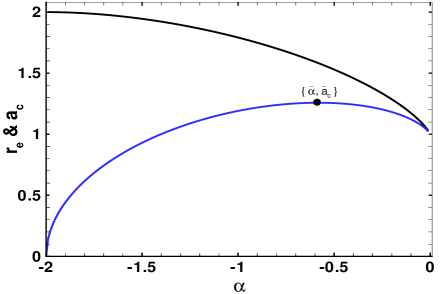
(a)

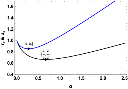
(b)

Figure 1: The horizon of the extremal black hole $r_{e}$ (black line) and critical values of the spin parameter $a_{c}$ (blue line) verse negative and positive $\alpha$ are plotted in panel (a) and (b). Here $\overline{\alpha}\approx-0.581977$, $\overline{a}_{c}\approx 1.25776655499709$, $\tilde{\alpha}=1/(1+e)$ and $\tilde{a}_{c}\approx 0.855$.

II.1 Negative $\alpha$

For any fixed chosen $\alpha<0$, the function $f(r,\alpha)$ has maxima at $r=-\alpha/{2}$. The function increases in the interval $0<r<-\alpha/2$ while decreases for $-\alpha/{2}<r$. Thus, depending on the value of $\alpha$, $f(r,\alpha)$ have no zero or have two zeros say $r_{1}$ and $r_{2}$ such that $r_{1}\leq-\frac{\alpha}{2}\leq r_{2}$. If $\alpha_{\text{min}}$ is the minimum value for which $f(r_{,}\alpha)$ has a zero, than

$$r_{1}=r_{2}\quad\text{for}\quad\alpha=\alpha_{\text{min}}.$$ (12)

That is, $r_{1}$ is a zero of $f(r,\alpha)$ of multiplicity $2$. Solving (8) for negative $\alpha$, we find that one zero of $f(r,\alpha)$ is

$$r_{1}=\frac{\alpha}{2}{ProductLog}\left({-2e^{-1+\frac{2}{\alpha}}}\right),$$ (13)

where $ProductLog(x)$ is a Lambert W-function. Now, if $r_{1}$ is zero of $f(r,\alpha)$ of multiplicity $2$, then it must also be zero of $df/dr$, which gives

$$\alpha_{\text{min}}=-\frac{2}{ln(2)}\approx-2.88539.$$ (14)

Note that for any value of $\alpha$ in the range $\alpha_{\text{min}}\leq\alpha<0$ the corresponding extremal value of $a$ are

$$a^{2}=r_{1}(r_{1}+\alpha)\quad and\quad a^{2}=r_{2}(r_{2}+\alpha).$$ (15)

As $r_{1}\leq-\alpha/2$, so in this case $a^{2}$ is negative which implies $r_{1}$ cannot be horizon of the extremal black hole and thus $r_{2}$ can be the horizon of the extremal black hole. Further, for $\alpha=-2$, $r_{2}=2$ and $a=0$. If $\alpha$ is in the range $-\alpha_{min}\leq\alpha<2$, the cosponsoring solution $r_{2}$ gives $a^{2}$ negative. Thus, for negative $\alpha$ the line element (1) represents a black hole only if $-2\leq\alpha<0$. Solving (8) numerically for $-2\leq\alpha<0$ gives horizon of the extremal black hole $r_{2}$ and henceforth will be represented by $r_{e}$. Using $r_{e}$ in (8), we get the critical value of spin parameter as follows

$$a_{c}=\sqrt{r_{e}(r_{e}+\alpha)}.$$ (16)

The graph of $r_{e}$ and $a_{c}$ for $-2\leq\alpha<0$ is plotted in FIG:1 (a) which shows that $r_{e}$ decreases with increasing $\alpha$, while $a_{c}$ has its maximum value $\overline{a}_{c}\approx 1.2577$ at $\overline{\alpha}\approx-0.58197$. If $\alpha$ is in the range, $-2\leq\alpha<\overline{\alpha}$ the critical value of spin parameter $a_{c}$ increases and if $\overline{\alpha}<\alpha<0$, then $a_{c}$ decreases. Further, as $r_{-}\leq r_{e}\leq r_{+}$ so we can say that for $-2\leq\alpha<0$, with increasing $\alpha$ the size of inner horizon $r_{-}$ decreases.

(a)

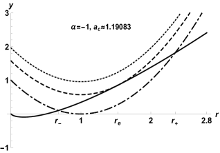
(b)

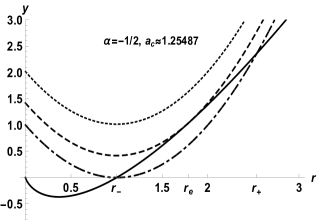
(c)

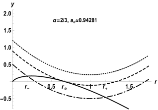
(d)

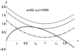
(e)

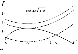
(f)

Figure 2: The graphs of $y=r^{2}-2r+a^{2}$ for different value of $a$, $a<a_{c}$ (dash-dotted line), $a=a_{c}$ (dashed line) and $a>a_{c}$ (dotted line) and $y=-\alpha rln(\frac{r}{|\alpha|})$ (solid line) are plotted. For any $\alpha$ and $a<a_{c}$, the point of intersection of solid lines and  dash-dotted parabolas in (a)-(f), give the locations of inner horizons $r_{-}$ and event horizons $r_{+}$. For $a=a_{c}$, the point of intersection of solid lines and dashed parabolas give the locations of horizon of extremal black hole $r_{e}$. For $a>a_{c}$, the solid line and dotted line does not intersect each other indicating that there does not exist a black hole and the line element (1) represents a naked singularity.

II.2 Case II: Positive $\alpha$

To discuss the critical value $a_{c}$ for any positive $\alpha$, we first find zeros of the function $f(r,\alpha)$. As for any chosen positive $\alpha$ the function $f(r,\alpha)$ is decreasing function of $r$ so it has at most one zero. Further

$$f(\overline{r}_{1},\alpha)=2>0\text{ \ with \ }\overline{r}_{1}=\frac{\alpha}{2}ProductLog\left(\frac{2}{e}\right),$$ (17)

and

$$f\left(\overline{r}_{2},\alpha\right)=-2\alpha e^{-1+\frac{2}{\alpha}}<0\text{ \ with \ }\overline{r}_{2}=\alpha e^{-1+\frac{2}{\alpha}},$$ (18)

By Intermediate value theorem we can conclude that for any $\alpha>0,$ $f\left(r,\alpha\right)$ has one zero (say $r_{e}$) such that $\overline{r}_{1}<r_{e}$ $<\overline{r}_{2}$. Solving (8) for $r$ yields

$$r_{e}=\frac{\alpha}{2}{ProductLog}\left({2e^{-1+\frac{2}{\alpha}}}\right).$$ (19)

and the corresponding extreme value of spin parameter $a_{c}$ is obtained as

$$a=\sqrt{r_{e}\left(2-r_{e}-\alpha\ln\left(\frac{r_{e}}{\alpha}\right)\right)},$$ (20)

or

$$a_{c}=\frac{\alpha}{2}\sqrt{ProductLog\left(2e^{-1+\frac{2}{\alpha}}\right)\left[2+ProductLog\left(2e^{-1+\frac{2}{\alpha}}\right)\right]},$$ (21)

The horizon of the extremal black hole $r_{e}$ and critical value of spin parameter $a_{c}$ verses $\alpha$ is plotted in FIG:1 (b) which shows that size of the extremal black hole has minimum value for $\alpha=2/3$. It decreases for $0<\alpha<2/3$ and increase for $2/3<\alpha$. For $\tilde{\alpha}=1/(1+e)$, $a_{c}$ has minimum value $\tilde{a}_{c}\approx 0.855$. Further, for $0<\alpha<\tilde{\alpha}$, $a_{c}$ decreases while $1/(1+e)<\alpha$ it increases.

We have plotted $y=r^{2}-2r+a^{2}$ for different values of $a$ and $y=-\alpha r\ln\left(\frac{r}{|\alpha|}\right)$ for negative $\alpha$ in FIG:2(a)-(c) and for positive $\alpha$ in FIG:2(d)-(f). In each case values of $r$ for which these curves intersect are horizons of the black hole. It is seen that for any value of $-2\leq\alpha$, if $a<a_{c}$ the curves intersect for two values of $r$ that are locations of inner horizon ($r_{-}$) and event horizon ($r_{+}$). If $a=a_{c}$ the horizons merge into a single horizon $r_{e}$ the horizon of extremal black hole and if $a>a_{c}$ the curve does not intersect each other that is no solution of horizon equation. Thus, we conclude that for any fixed $-2\leq\alpha$ the line element (1) represents a black hole with two horizons $\ r_{-}$ and $r_{+}$ only if $a<a_{c}$. For $a=a_{c}$, the two horizons $r_{+}$ and $r_{-}$ merge into a single horizon $r_{e}$ and (1) is a extremal black hole. However, for any $a>a_{c}$, the line element is a naked singularity.

III Spin Precession Frequency

In this section, we will discuss the spin precession frequency of a test gyroscope attached to a stationary observer with respect to some fixed star due to the frame dragging effects of the Kerr-like black hole in the PFDM. The precession frequency ($\Omega_{p}$) of a test gyroscope attached to a stationary observer having $4-$ velocity $u=(-K^{2})^{-1/2}K$ in a stationary spacetime with timelike Killing vector field $K=\partial_{0}+\Omega\partial_{t}$ is defined by NS

$$\vec{\Omega}_{p}=\frac{\varepsilon_{ckl}}{2\sqrt{-g}\left(1+2\Omega\frac{g_{0c}}{g_{00}}+\Omega^{2}\frac{g_{cc}}{g_{00}}\right)}\left[\left(g_{0c,k}-\frac{g_{0c}}{g_{00}}g_{00,k}\right)+\Omega\left(g_{cc,k}-\frac{g_{cc}}{g_{00}}g_{00,k}\right)+\Omega^{2}\left(\frac{g_{0c}}{g_{00}}g_{cc,k}-\frac{g_{cc}}{g_{00}}g_{0c,k}\right)\right]\partial_{l},$$ (22)

where $\varepsilon_{ckl}$ is the Levi-Civita symbols and $g$ is the determinant of the metric $g_{\mu\nu}$. Using the metric coefficients from (1) in (22) yields

$$\vec{\Omega}_{p}=\frac{\left(F\sqrt{\Delta}\cos\theta\right)\hat{r}\text{ }+\left(H\sin\theta\right)\hat{\theta}\text{ }}{\Sigma^{3/2}\left[\Sigma-\left\{2Mr-\alpha r\ln\left(\frac{r}{|\alpha|}\right)\right\}\left(1-2\Omega a\sin^{2}\theta\right)-\Omega^{2}\sin^{2}\theta\left\{\left(r^{2}+a^{2}\right)\Sigma+a^{2}\sin^{2}\theta\left(2Mr-\alpha r\ln\left(\frac{r}{|\alpha|}\right)\right)\right\}\right]},$$ (23)

where

$$F = a\left\{2Mr-\alpha r\ln\left(\frac{r}{|\alpha|}\right)\right\}-\frac{\Omega}{8}\left\{3a^{4}+8r^{4}+8a^{2}r\left(2M+r\right)+a^{2}\left(a^{2}\cos 4\theta-8\alpha r\ln\left(\frac{r}{|\alpha|}\right)+4\cos 2\theta\left(2\Delta-a^{2}\right)\right)\right\}$$ (24)

$$+\Omega^{2}a^{3}\left\{2Mr-\alpha r\ln\left(\frac{r}{|\alpha|}\right)\right\}\sin^{4}\theta,$$

$$H = a\left[M\left(r^{2}-a^{2}\cos^{2}\theta\right)+\frac{\alpha}{2}\left\{\Sigma-\left(r^{2}-a^{2}\cos^{2}\theta\right)\ln\left(\frac{r}{|\alpha|}\right)\right\}\right]$$ (25)

$$+\Omega\left[a^{4}r\cos^{4}\theta+r^{2}\left(r^{3}-a^{2}M\left(1+\sin^{2}\theta\right)-3Mr^{2}\right)+a^{2}\cos^{2}\theta\left\{2r^{3}+a^{2}M\left(1+\sin^{2}\theta\right)-Mr^{2}\right\}\right.$$

$$\left.-\frac{\alpha}{16}\left\{a^{2}\left(5a^{2}+16r^{2}\right)+8r^{4}+\left(5a^{4}-16a^{2}r^{2}-24r^{4}\right)\ln\left(\frac{r}{|\alpha|}\right)+a^{4}\left(4\cos 2\theta-\cos 4\theta\right)\left\{1+\ln\left(\frac{r}{|\alpha|}\right)\right\}\right\}\right]$$

$$+a\Omega^{2}\sin^{2}\theta\left[M\left\{r^{2}\left(3r^{2}+a^{2}\right)+a^{2}\cos^{2}\theta\left(r^{2}-a^{2}\right)\right\}+\frac{\alpha}{2}\left\{a^{2}\cos^{2}\theta\left\{r^{2}+a^{2}+\left(a^{2}-r^{2}\right)\ln\left(\frac{r}{|\alpha|}\right)\right\}\right.\right.$$

$$\left.\left.+r^{2}\left\{r^{2}+a^{2}-\left(3r^{2}+a^{2}\right)\ln\left(\frac{r}{|\alpha|}\right)\right\}\right\}\right],$$

and $\hat{r}$, $\hat{\theta}$ are the unit vectors in $r$ and $\theta$ directions, respectively. In the limiting case $\alpha=0$, the spin precession of a Kerr black hole is successfully obtained NS . Note that the above expression of the precession frequency (22) is valid only for a timelike observer at fixed $r$ and $\theta$ which gives the restriction on the angular velocity $\Omega$ of the observer

$$\Omega_{-}(r,\theta)<\Omega(r,\theta)<\Omega_{+}\left(r,\theta\right),$$ (26)

with

$$\Omega_{\pm}=\frac{a\sin\theta\left\{2Mr-\alpha r\ln\left(\frac{r}{|\alpha|}\right)\right\}\pm\Sigma\sqrt{\Delta}}{\sin\theta\left[\left(r^{2}+a^{2}\right)\Sigma+a^{2}\sin^{2}\theta\left\{2Mr-\alpha r\ln\left(\frac{r}{|\alpha|}\right)\right\}\right]}.$$ (27)

At the black hole horizons, $\Omega_{+}$ and $\Omega_{-}$ coincide and no timelike observer can exist there and hence the expression for precision frequency $\Omega_{p}$ is not valid at the horizons but still we can study the behavior of precession frequency near the black hole horizon.

III.1 Lense-Thirring precession frequency

The expression of the precession frequency (23) is valid for all the stationary observers inside and outside the ergosphere if their angular velocity $\Omega$ is in the restricted range given by (26). The precession frequency contains the effects because of the spacetime rotation (LT precession) as well as due to spacetime curvature (geodetic precession). If we set $\Omega=0$ in (23), the expression for LT precession frequency for Kerr-Like black hole in PFDM is obtained as

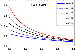
(a)

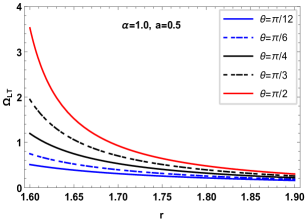
(b)

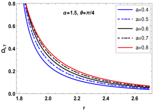
(c)

Figure 3: The LT precession frequency $\Omega_{LT}$ (in $M^{-1}$ ) verse $r$ (in $M$) for different parameters is plotted.

$$\vec{\Omega}_{LT}=a\frac{\left[2Mr-\alpha r\ln\left(\frac{r}{|\alpha|}\right)\right]\sqrt{\Delta}\cos\theta\hat{r}\text{ }+\sin\theta\left[M\left(r^{2}-a^{2}\cos^{2}\theta\right)+\frac{\alpha}{2}\left\{\Sigma-\left(r^{2}-a^{2}\cos^{2}\theta\right)\ln\left(\frac{r}{|\alpha|}\right)\right\}\right]\hat{\theta}\text{ }}{\Sigma^{3/2}\left[\Sigma-\left\{2Mr-\alpha r\ln\left(\frac{r}{\alpha}\right)\right\}\right]}.$$ (28)

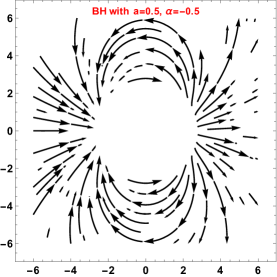
(a)

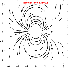
(b)

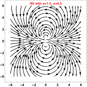
(c)

Figure 4: The vector field of the LT- precession frequency (28) (in Cartesian plane corresponding to $(r,\theta)$) for black holes is plotted in panels (a) and (b) for negative and positive $\alpha$ and for naked singularity in panel (c). The field lines show that for black hole the vector field is defined outside the ergoshpere only, while for naked singularities it is finite up to the ring singularity along all the directions.

The magnitude of the LT precession frequency is given by

$$\Omega_{LT}=a\frac{\sqrt{\left[2Mr-\alpha r\ln\left(\frac{r}{|\alpha|}\right)\right]^{2}|\Delta|\cos^{2}\theta\text{ }+\left[M\left(r^{2}-a^{2}\cos^{2}\theta\right)+\frac{\alpha}{2}\left\{\Sigma-\left(r^{2}-a^{2}\cos^{2}\theta\right)\ln\left(\frac{r}{|\alpha|}\right)\right\}\right]^{2}\sin^{2}\theta}\text{ }}{\Sigma^{3/2}\left|\Sigma-\left\{2Mr-\alpha r\ln\left(\frac{r}{|\alpha|}\right)\right\}\right|}.$$ (29)

The magnitude of LT precession frequency $\Omega_{LT}$ is plotted against $r$ in the FIG: (3), which indicates that the LT precession frequency increases with increasing the rotation $a$ of the black hole as well as the dark energy parameter $\alpha$. Further, for $\alpha>0$ the LT precession frequency is minimum near polar axis ($\theta=0$) and increases towards the equatorial plane ($\theta=\pi/2$) whereas for $\alpha<0$ it is minimum in equatorial plane and increases towards the polar axis. The vector field of the LT-precession frequency for the black hole and naked singularity in FIG:(4) which shows that LT precession frequency for the black hole remains finite outside the ergoregion and will diverge at ergoregion while for naked singularity it remains finite up to the ring singularity.

IV Geodetic precession

For $a=0$, the line element (1) reduces to the Schwarzschild black hole in PFDM SCindark . The Schwarzschild black hole in PFDM is non rotating and have zero precession due to the frame dragging effects. However, due to spacetime curvature the precession frequency $\Omega_{p}$ of a test gyroscope is nonzero which is because of curvature of spacetime and called geodetic precession frequency. The geodetic precession effects can be obtained as

$$\vec{\Omega}_{p}|_{a=0}=\Omega\frac{\left(-\cos\theta\sqrt{r^{2}-2Mr+\alpha r\left(\frac{r}{|\alpha|}\right)}\right)\hat{r}+\sin\theta\left(r-3M-\frac{\alpha}{2}\left\{1-3\ln\left(\frac{r}{|\alpha|}\right)\right\}\right)\hat{\theta}}{r-2M+\alpha\ln\left(\frac{r}{|\alpha|}\right)-\Omega^{2}r^{3}\sin^{2}\theta}.$$ (30)

Due to spherically symmetric geometry of the static black hole in the PFDM the geodetic precession frequency is same over any spherical symmetric surface around the black hole. Thus, without loss of generality we can set $\theta=\pi/2$ and study the geodetic frequency in equatorial plane. In this plane for any observer in circular orbit the magnitude of precession frequency is equal to the Kepler frequency given by

$${\Omega}_{p}|_{a=0}\equiv\Omega_{\text{Kep}}=\left[\frac{M}{r^{3}}+\frac{\alpha}{2r^{3}}\left\{1-\ln\left(\frac{r}{|\alpha|}\right)\right\}\right]^{1/2}.$$ (31)

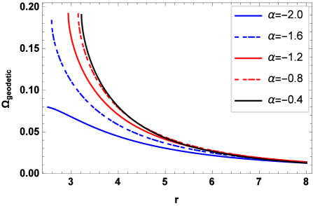
(a)

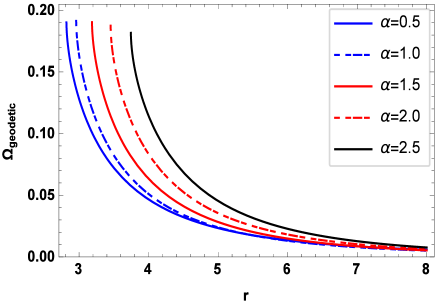
(b)

Figure 5: The geodetic precession frequency $\Omega_{\text{geodetic}}$ verse $r$ for $\alpha<0$ in panel (a) and for $\alpha>0$ in panel (b) is plotted which shows that the geodetic precession frequency increases with increasing $\alpha$.

The above expression for precession frequency is valid for Copernican frame a frame that does not rotate relative to the inertial frame at asymptotic infinity i.e. the fixed stars, computed with respect to proper time $\tau$ which is related with the coordinate time $t$ via

$$d\tau=\sqrt{1-\frac{3M}{r}-\frac{\alpha}{2r}\left\{1-\ln\left(\frac{r}{|\alpha|}\right)\right\}}dt.$$ (32)

Using this transformation the geodetic precession frequency associated with the change in the angle of the spin vector after one complete revolution of the observer around a black hole in the coordinate basis is given by

$$\Omega_{\text{geodetic}}=\left[\frac{M}{r^{3}}+\frac{\alpha}{2r^{3}}\left\{1-\ln\left(\frac{r}{|\alpha|}\right)\right\}\right]^{1/2}\left(1-\sqrt{1-\frac{3M}{r}-\frac{\alpha}{2r}\left\{1-\ln\left(\frac{r}{|\alpha|}\right)\right\}}\right).$$ (33)

In this absence of PFDM around the black hole that is for $\alpha=0$, the geodetic precession frequency for a Schwarzschild black hole successfully recovered geosc1 ; geosc2 . The geodetic precession frequency is plotted against $r$ for negative and positive $\alpha$ in panel $(a)$ and $(b)$ of FIG: (3), which shows that with increasing PFDM parameter $\alpha$ the magnitude of the geodetic precession frequency increases. Further, for any fixed $\alpha$ the geodetic precession frequency decreases with increasing the radius of the circular orbit.

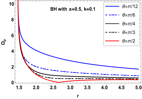
(a)

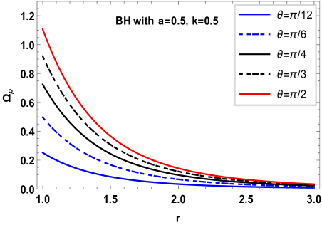
(b)

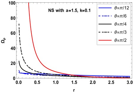
(c)

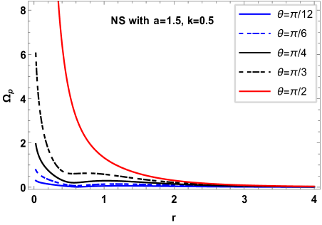
(d)

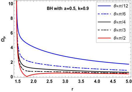
(e)

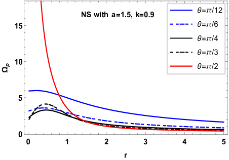
(f)

Figure 6: We have plotted the magnitude of spin precession frequency $\Omega_{p}$ (in $M^{-1}$ ) verse $r$ (in $M$) is plotted for black hole in left column and for naked singularity in right column. For black hole we take $a=0.5$, $\alpha=1$ and for naked singularity we take $a=1.5$ and $k=0.1,0.5,0.9$ in first, second and third row, respectively. For black hole the precession frequency $\Omega_{p}$ diverges for $k=0.1,0.9$ and remain finite for $k=0.5$ as the observer approaches the event horizon along any direction, whereas for naked singularity case it with remain finite along all direction except at ring singularity ($r=0$, $\theta=\pi/2$).

V Distinguishing black hole from naked singularity

In this section, using the precession frequency of a gyroscope, we will differentiate a Kerr-like black hole in PFDM from naked singularity and verify our results as obtained in section II. For this we first express the angular velocity of the timelike observer in term of a parameter $k$ such that

$$\Omega=k\Omega_{+}+(1-k)\Omega_{-},$$ (34)

where $0<k<1$ and $\Omega_{\pm}$ given by (27). Thus for any timelike observer the angular velocity defined as

$$\Omega=\frac{a\sin\theta\left\{2Mr-\alpha r\ln\left(\frac{r}{|\alpha|}\right)\right\}-\left(1-2k\right)\Sigma\sqrt{\Delta}}{\sin\theta\left[\left(r^{2}+a^{2}\right)\Sigma+a^{2}\sin^{2}\theta\left\{2Mr-\alpha r\ln\left(\frac{r}{|\alpha|}\right)\right\}\right]},$$ (35)

Note that an observer with angular velocity parameter $k=1/2$ is known as zero-angular-momentum observer (ZAMO) and has an angular velocity

$$\Omega=-\frac{g_{t\phi}}{g_{\phi\phi}}=\frac{a\left\{2Mr-\alpha r\ln\left(\frac{r}{|\alpha|}\right)\right\}}{\left(r^{2}+a^{2}\right)\Sigma+a^{2}\sin^{2}\theta\left\{2Mr-\alpha r\ln\left(\frac{r}{|\alpha|}\right)\right\}},$$ (36)

The gyroscope attached to ZAMO observer is locally nonrotating and useful to study physical procession near astrophysical objects Bardeen . Further, the behavior of the precession frequency attached to ZAMO observer is different from the all other observers this situation is explain in FIG: (6). Now the magnitude of the precession frequency $\Omega_{p}$ in term of parameter $k$ is written as

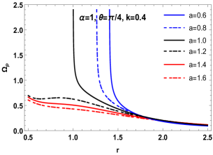
(a)

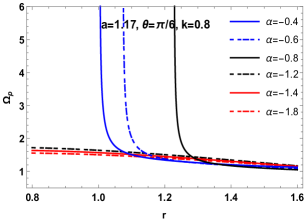
(b)

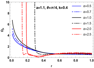
(c)

Figure 7: The precession frequency $\Omega_{p}$ (in $M^{-1}$ ) verse $r$ (in $M$) for different parameters is plotted. The graphs show that for black holes $\Omega_{p}$ diverges near the horizons while for naked singularities it remain finite.

$$\Omega_{p}=\frac{\left|\left(r^{2}+a^{2}\right)\Sigma+a^{2}\sin^{2}\theta\left(2Mr-\alpha r\ln\left(\frac{r}{|\alpha|}\right)\right)\right|}{4\Sigma^{7/2}k\left(1-k\right)\left|\Delta\right|}\left[F^{2}|\Delta|\cos^{2}\theta+H^{2}\sin^{2}\theta\right]^{1/2}.$$ (37)

where $F$ and $G$ are given by (24) and (25). From the denominator of the above equation one can see that it vanishes at the horizons of the black hole and ring singularity. Thus we study the behavior of $\Omega_{p}$ for different values of spacetime parameters $a$ and $\alpha$ and observer’s angular velocity parameter $k$ in detail.

In FIG: (6), we have plotted $\Omega_{p}$ for black hole with $a=0.5$ and $\alpha=1$ in left column and for naked singular with $a=1.5$ and $\alpha=1$ in right column for different observers of angular velocity parameter $k=0.1,0.5,0.9$ in first, second and third row, respectively. It is seen that for a black hole the precession frequency $\Omega_{p}$ of a gyroscope attached to any observer except ZAMO, diverges when ever it approach the horizons along any direction. However, its remain finite for ZAMO observer at horizon. On the other hand, for a naked singularity the precession frequency remain finite even as the observer approach $r=0$ along any direction except $\theta=\pi/2$. Further, if the observer approach $r=0$ along $\theta=\pi/2$ the precession frequency $\Omega_{p}$ becomes very large because of the ring singularity. In FIG: (7), we further illustrate that for all other choices of the parameters, the behavior of the precession frequency $\Omega_{p}$ remain the same as in case of the black hole with $a=0.5$ and $\alpha=1$ and $a=1.5$ and $\alpha=1$ in naked singularity. That is, for black hole with any $a$ and $\alpha$ the precession frequency $\Omega_{p}$ of gyroscope of all the observer except ZAMO, diverges near the horizons while for naked singularity it remain finite up to $r=0$ along any direction except $\theta=\pi/2$.

Finally, using the spin precession frequency of a test gyroscope attached to stationary observer, we can differentiate a black hole from naked singularity. The four velocity of an observer in the spacetime of the line element (1) is timelike if azimuthal components of the velocity (equal to angular velocity) $\Omega$ at fixed $(r,\theta)$ remain in between $\Omega_{-}$ and $\Omega_{+}$. Further, the angular velocity can be parameterized $q$ such that $0<q<1$. Consider there are two observer with different angular velocity $\Omega_{1}$ and $\Omega_{2}$ approaching the astrophysical object in the PFDM of line element (1) along the different directions $\theta_{1}$ and $\theta_{2}$. If (a) the precession frequency $\Omega_{p}$ of a test gyroscope of at least one observer becomes arbitrary large as the observer approach the central object along any direction then the object is a black hole and (b) if the precession frequency of any of the observer along at most one of the two directions becomes arbitrarily larges as it approach the central object, then the object is a naked singularity.

VI Observational aspects

Experimental observations obtained with the Rossi X-ray Timing Explorer (RXTE) reveals the phenomena of quasi-periodic oscillations (QPOs) by analyzing the power spectrum of the time series of the X-rays stella1 ; stella2 ; xray2 ; Revnew . There are various sources of cosmic X-rays and one of them is accreting stellar mass near compact objects like black holes and neutron stars. A careful monitoring identifies two types of QPOs, namely the high-frequency quasi-periodic oscillations (HF QPOs), and the low-frequency (LF QPOs). Although the theoretical explanation behind this effect is not yet well understood, QPOs are often linked with the relativistic precession of the accretion disk near black holes or neutron stars. QPOs may be potentially a useful tool in astrophysics for investigating new features related to the accretion process near black holes. For example, within a certain model of X-ray timing measurements of QPOs can be used to estimate the spin angular momentum and the mass of the black hole which is of significant importance in astrophysics motta . Experimental data shows that, the observed HF QPOs belong to the interval $50-450$ Hz. Furthermore, there are three classes of LF QPOs known as: type-A, type-B, and type-C, LF QPOs, respectively. The typical frequencies belong to the interval: $6.5-8$Hz, $0.8-6.4$ Hz, and $0.01-30$ Hz, respectively.

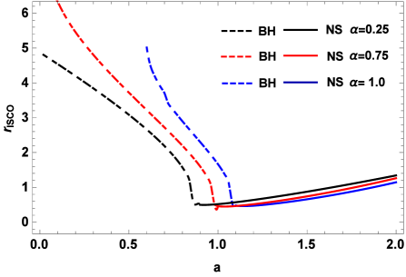
(a)

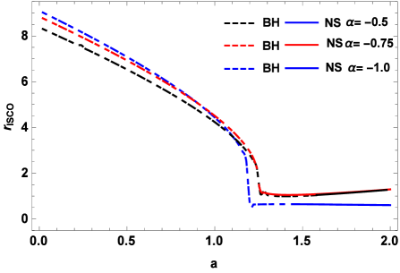
(b)

Figure 8: The ISCO of the black hole (BH) and naked singularity (NS) (in the unit of $M$) for positive and negative PFDM parameter $\alpha$ is plotted in panel (a) and (b), respectively. For $\alpha=-0.5,-0.75,-1.0$, the critical values of spin parameter are $a_{c}=1.25486557,1.246502349,1.190826462$ and for positive values of $\alpha$ the critical value of $a_{c}$ is obtained from (21).

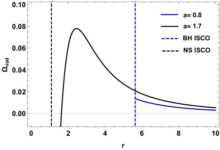
(a)

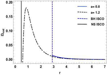
(b)

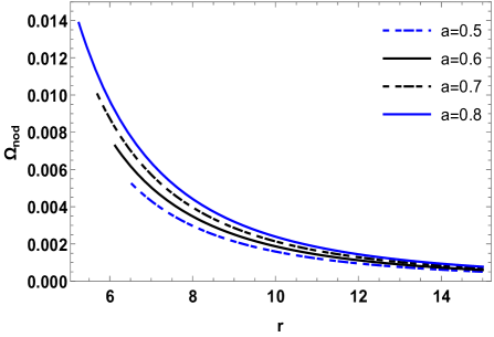
Figure 9: We plot $\Omega_{nod}$ (in units of $M^{-1}$) as a function of $r$ (in units of $M$) with $\alpha=-1$ and $\alpha=1$. As can be seen, for black holes the NPPF $\Omega_{nod}$ decreases as we increase $r$. From the plots we can further observe that a naked singularity is characterized by a peak value of $\Omega_{nod}$. Furthermore $\Omega_{nod}$ vanishes at some radius $r_{0}$. The negative values of $\Omega_{nod}$, physically can be interpreted as a reversion of the precession direction.

(c)

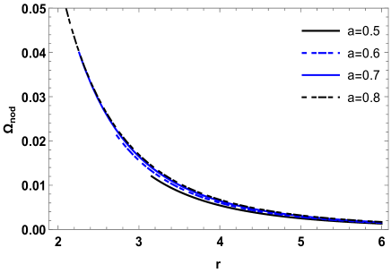
(d)

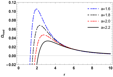
Figure 10: We plot the NPPF $\Omega_{nod}$ as a function of $r$ for the black hole case with $\alpha=-0.5$ and $\alpha=0.5$. Clearly $\Omega_{nod}$ always decreases with the increase of $r$.

(e)

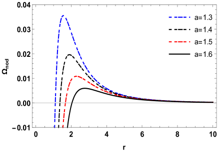
(f)

Figure 11: The $\Omega_{nod}$ as a function of $r$ is plotted in the case of naked singularities with $\alpha=-0.5$ and $\alpha=0.5$. From the plots we can see that $\Omega_{nod}$ increases initially, then a particular peak value is obtained, and finally decreases with the increase of $r$. The negative values of $\Omega_{nod}$, shows that the precession direction has changed.

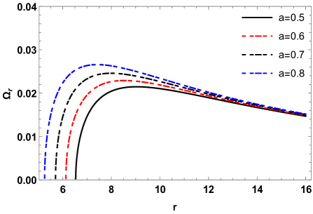
(a)

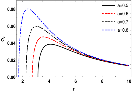
(b)

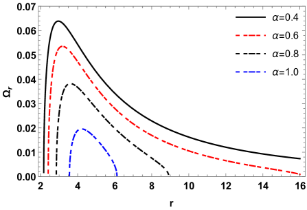
(c)

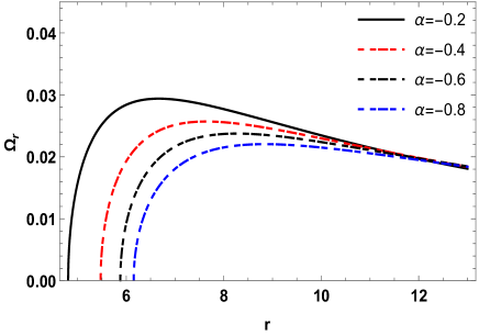
(d)

Figure 12: We plot $\Omega_{r}$ versus $r$ with PFDM parameter values (upper panel) $\alpha=-1$ and $\alpha=1$, and spin parameter (lower panel) $a=-0.7$ and $a=0.7$. We can see that $\Omega_{r}$ vanishes at some particular value of $r$ depending on the particular value of PFDM parameter. Note that, $\Omega_{r}$ reaches a particular peak value, then decreases with the increase of $r$.

		$\alpha=1$ (in $M$)			$\alpha=0.5$ (in $M$)			$\alpha=0$ (in $M$)
$a/M$	$r$ (in $M$)	$\nu^{\alpha}_{\phi}$ (in Hz)	$\nu^{\alpha}_{\theta}$ (in Hz)	$\nu^{\alpha}_{\text{nod}}$ (in Hz)	$\nu^{\alpha}_{\phi}$ (in Hz)	$\nu^{\alpha}_{\theta}$ (in Hz)	$\nu^{\alpha}_{\text{nod}}$ (in Hz)	$\nu^{0}_{\phi}$ (in Hz)	$\nu^{0}_{\theta}$ (in Hz)	$\nu^{0}_{\text{nod}}$ (in Hz)
0.1	5.67	220	217	3	226	223	3	234	231	3
0.2	5.45	232	226	6	238	231	7	246	239	7
0.3	5.32	239	229	10	245	234	10	253	242	11
0.4	4.61	192	273	19	299	279	20	309	287	22
0.5	4.30	320	293	27	333	302	31	344	310	34
0.6	3.82	375	331	44	383	336	47	395	342	53
0.7	3.45	527	363	64	435	366	69	448	371	77
0.8	2.85	544	428	116	553	428	125	567	429	138
0.9	2.32	693	491	202	702	483	219	718	472	246
0.98	1.85	884	544	340	893	521	372	910	485	425
0.99	1.45	1137	575	562	1146	520	626	1163	420	743
0.9999	1.20	1350	593	757	1358	498	860	1375	276	1099
0.999999	1.05	1509	635	874	1517	507	1010	1533	89	1444
1.0	1	1568	669	899	1575	532	1043	1591	0	1591
1.001	0.95	1629	724	905	1636	583	1053	1652	133	1519
1.01	0.80	1825	1093	732	1830	968	862	1844	679	1165
1.02	0.75	1888	1339	549	1954	1428	526	1967	1199	768
1.04	0.65	2020	2025	-5	2024	1941	83	2035	1753	282
1.08	0.667	1944	2127	-183	1948	2054	-106	1959	1894	65
1.2	0.8	1646	1863	-217	1650	1808	-158	1662	1696	-34
2	1.26	919	1619	-700	923	1609	-686	932	1588	-656
3	3.20	353	453	-100	357	453	-96	365	453	-88
4	4.00	256	371	-115	260	373	-113	265	375	-110

		$\alpha=-1$ (in $M$)			$\alpha=-0.5$ (in $M$)			$\alpha=-0.1$ (in $M$)
$a/M$	$r$ (in $M$)	$\nu^{\alpha}_{\phi}$ (in Hz)	$\nu^{\alpha}_{\theta}$ (in Hz)	$\nu^{\alpha}_{\text{nod}}$ (in Hz)	$\nu^{\alpha}_{\phi}$ (in Hz)	$\nu^{\alpha}_{\theta}$ (in Hz)	$\nu^{\alpha}_{\text{nod}}$ (in Hz)	$\nu^{\alpha}_{\phi}$ (in Hz)	$\nu^{\alpha}_{\theta}$ (in Hz)	$\nu^{\alpha}_{\text{nod}}$ (in Hz)
0.1	5.67	247	243	4	242	238	4	236	233	3
0.2	5.45	259	251	8	254	246	8	248	241	7
0.3	5.32	267	254	13	261	249	12	255	244	11
0.4	4.61	325	299	26	318	294	24	312	289	23
0.5	4.30	354	317	37	348	312	35	341	307	34
0.6	3.82	412	352	60	406	349	57	398	344	54
0.7	3.45	467	378	89	460	376	84	451	372	79
0.8	2.85	589	427	162	581	429	152	571	429	141
0.9	2.32	741	449	292	733	460	273	722	469	253
0.98	1.85	935	410	525	926	443	483	925	474	441
0.99	1.45	1188	113	1075	1180	281	899	1169	387	782
0.9999	1.60	1070	315	762	1069	384	685	1058	455	613
0.999999	1.50	1147	224	923	1138	330	808	1127	415	1712
1.0	1.55	1111	277	834	1138	330	808	1089	432	660
1.001	1.95	879	423	455	870	450	420	859	475	384
1.01	1.80	954	398	555	945	436	509	934	472	462
1.02	1.75	978	386	592	970	429	541	959	470	489
1.04	1.65	1032	357	675	1023	413	610	1012	464	548
1.08	1.667	1008	378	630	1000	430	570	980	478	512
1.2	1.8	902	437	465	895	472	422	985	506	378
2	1.26	944	1550	-606	941	1565	-624	935	1518	-646
3	3.20	376	449	-73	372	451	-79	367	457	-85
4	4.00	274	377	-103	271	377	-106	267	375	-108

Table 1: We have considered an object with mass $M=10{M}_{\odot}$ to calculate the KF precession $\nu^{\alpha}_{\theta}$, VEF precession $\nu^{\alpha}_{\theta}$, and the NPPF $\nu^{\alpha}_{\text{nod}}$, respectively. We have chosen the ISCO radius $r=r_{ISCO}$ given by the interval $M\leq r_{ISCO}\leq 6M$.

There are three characteristic frequencies attributed to a test particle orbiting the black hole, namely the KF $\Omega_{\phi}$, the VEF $\Omega_{\theta}$, and the radial epicyclic frequency (REF) $\Omega_{r}$, respectively. By taking into account the effect of PFDM we have calculated the following expressions for the characteristic frequencies kepfreq :

$$\Omega_{\phi} = \pm\frac{\sqrt{M+\frac{\alpha}{2}\left(1-\ln\left(\frac{r}{|\alpha|}\right)\right)}}{r^{3/2}\pm a\sqrt{M+\frac{\alpha}{2}\left(1-\ln\left(\frac{r}{|\alpha|}\right)\right)}},$$ (38)

$$\Omega_{r} = \frac{\Omega_{\phi}}{r}\left[r^{2}-6Mr-3a^{2}-\alpha r\left\{1-3\ln\left(\frac{r}{|\alpha|}\right)\right\}\pm 8a\sqrt{rM+\frac{\alpha r}{2}\left\{1-\ln\left(\frac{r}{|\alpha|}\right)\right\}}-\frac{\alpha\left\{a^{2}+ar+r^{2}\right\}}{\left\{2M+2\alpha\left(1-\ln\left(\frac{r}{|\alpha|}\right)\right)\right\}}\right]^{\frac{1}{2}},$$ (39)

$$\Omega_{\theta} = \frac{\Omega_{\phi}}{r}\left[r^{2}+3a^{2}\mp 4a\sqrt{rM+\frac{\alpha r}{2}\left\{1-\ln\left(\frac{r}{|\alpha|}\right)\right\}}-\frac{a\alpha\left\{a\mp 2\sqrt{rM+\frac{\alpha r}{2}\left\{1-\ln\left(\frac{r}{|\alpha|}\right)\right\}}\right\}}{\left\{M+\frac{\alpha}{2}\left(1-\ln\left(\frac{r}{|\alpha|}\right)\right)\right\}}\right]^{\frac{1}{2}}.$$ (40)

One can easily show that in the limiting case when $\alpha$ vanishes, the characteristic frequencies in the Kerr geometry are obtained NS ; mottanew ; bambi . With these results in mind, we can extract further informations by defining the following two quantities

$$\Omega_{\text{nod}}=\Omega_{\phi}-\Omega_{\theta},$$ (41)

and

$$\Omega_{\text{per}}=\Omega_{\phi}-\Omega_{r}.$$ (42)

Where $\Omega_{\text{nod}}$ measures the orbital plane precession and is usually known as the NPPF (or Lense-Thirring precession frequency), on the other hand $\Omega_{\text{per}}$ measures the precession of the orbit and is known as the periastron precession frequency. From FIG. (9)-(11) we can see that in the black hole case, the NPPF $\Omega_{nod}$ always decreases with $r$, therefore we can write the following condition

$$\frac{d\Omega_{nod}}{dr}<0.$$ (43)

On the other hand, an interesting feature arises in the case of naked singularities, namely $\Omega_{nod}$ initially increases, then a particular peak value is recovered, and finally $\Omega_{nod}$ decreases with the increase of $r$. Therefore, in the case of naked singularities we can have the following condition when $\Omega_{nod}$ increases with with $r$, written as follows

$$\frac{d\Omega_{nod}}{dr}>0.$$ (44)

Finally we point out that negative values of $\Omega_{nod}$, can be interpreted as a reversion of the precession direction.

We provide a detailed analyses of our results in Table I, where we highlight the observational aspects by calculating the impact of the PFDM parameter on different frequencies: KF $\nu^{\alpha}_{\theta}$, VEF $\nu^{\alpha}_{\theta}$, and the NPPF $\nu^{\alpha}_{\text{nod}}$. Our results reveal that, typical values of the PFDM parameter $\alpha$ significantly affects these frequencies. In particular we find that, with the increase of positive $\alpha$, all frequencies become smaller and smaller. On the other hand, with the decrease of negative $\alpha$, all frequencies become bigger and bigger. Our results further indicate that, the effects of PFDM are getting stronger with the increase of spin angular momentum parameter $a$. From the Table I, we see that one can identify LF QPOs with $\nu_{\text{nod}}^{\alpha}$, for a slowly rotating black holes, i.e $a/M<0.5$. A significant difference between $\nu^{\alpha}_{\text{nod}}$ and $\nu^{0}_{\text{nod}}$, occurs when $a/M>0.5$. Clearly, in this range, we can identify $\nu^{\alpha}_{\text{nod}}$ with HF QPOs. In the near future we plan to investigate the relativistic precession model to get constraints on $\alpha$ using the data of GRO J1655-40 and by following the analysis presented by Bambi bambi .

VII Conclusion

In this paper, we have studied rotating object in PFDM (1) to differentiate a Kerr-like black hole from naked singularity. For a black hole we find the lower bound of the dark matter parameter $\alpha$, $-2\leq\alpha$ and gives the critical value of spin parameter $a_{c}$. For any fixed chosen $\alpha$ the line element (1) represents a black hole with two horizons if $a<a_{c}$, extremal black hole with one horizon if $a=a_{c}$ and naked singularity if $a>a_{c}$. It is seen that for $\alpha<0$, $a_{c}$ has maxima at $\alpha=\overline{\alpha}$ and for $\alpha>0$ it has minima at $\alpha=\tilde{\alpha}$. Further, for large value of $\alpha$, $a_{c}$ increases very large without any limit and thus a highly spinning black hole can form. We also study the horizon of extremal black hole and find that for $\alpha<0$ the size of extremal horizon $r_{e}$ decrease whereas for $\alpha>0$, $r_{e}$ has minima at $\alpha=2/3$. Further, as $r_{-}\leq r_{e}\leq r_{+}$, so we can conclude that for any fixed $a$ and $-2\leq\alpha<2/3$, with increasing $\alpha$, size of the black hole horizons decreases while for $2/3<\alpha$ increases.

We also studied the spin precession frequency $\Omega_{p}$ of the a test gyroscope attached to a stationary timelike observer. For timelike observer we find the restricted domain for the angular velocity $\Omega$ of the observer. From the precession frequency $\Omega_{p}$, by setting $\Omega=0$, we obtained LT- precession frequency for a static observer which can lies only outside the ergosphere. We also find the geodetic precession frequency which is due to the of spacetime curvature of Schwarzschild black hole in PFDM. It is seen that for $\alpha<0$ the geodetic precession frequency is increases while for $\alpha>0$ is increases.

Using spin precession frequency criteria we differentiate a black hole from a naked singularity. We parameterize the angular velocity of the observer and studied the spin precession frequency for different choices of the parameter along the different directions. If the precession frequency of a gyroscope attached to at least one of two observers with different angular velocities blow up if they approach the central object in PFDM along any direction then the object is a black hole. If the precession frequency of all the observer show divergence as the observers approach the center of spacetime along at most one direction then it is naked singularity.

We have summarized our results by computing the effect of PFDM on the KF, VEF, and NPPF given in Table I. We observe that frequencies depend upon the value of $a/M$, radial distance $r$, as well as the PFDM parameter $\alpha$, yielding notable differences in the corresponding frequencies of black holes and naked singularities. We have shown that, with the increase of positive PFDM parameter, all frequencies become smaller. Consequently, with the decrease of negative PFDM parameter, all frequencies become bigger. Following our results we can conclude that LF QPOs can be identified for $a/M<0.5$. However, most significant changes are observed in the interval $a/M>0.5$, whose frequencies can be identified with HF QPOs.

Given the fact that the accretion disk changes with time, say, when the accretion disk approaches the black hole/naked singularity, we need to study the evolution of QPO frequencies to distinguish black holes from naked singularities. In particular, for a given value of PFDM parameter $\alpha$ and $a/M$, if the accretion disc approaches the $r_{ISCO}$, we see that $\Omega_{nod}$ always increases reaching its maximum value. Interestingly, in the case of naked singularities, if the accretion disc approaches the $r_{ISCO}$, we find that $\Omega_{nod}$ firstly increases, then reaches its peak, and finally decreases. In fact, contrary to the black holes, in the case of naked singularity $\Omega_{nod}$ can be zero, as can be seen from FIG. (9). Finally, we anticipate that future experiments could produce constraints for the PFDM parameter $\alpha$. For example, recently Bhattacharyya has proposed a model of fast radio bursts from neutron stars plunging into black hole that implies the existence of event horizon, LT effects and the emission of gravitational waves from a black hole bhattacharyya . In this context, it would certainly be interesting to explore the possible impact of the PFDM parameter $\alpha$ on the gravitational wave signatures.

- (1) V. C. Rubin, Jr. W. K. Ford and N. Thonnard,Astro. Phys. J. 238, 471 (1980).
- (2) F. Zwicky, Helvetica Physica Acta, 6, 110 (1933).
- (3) Planck Collaboration: P. A. R. Ade, N. Aghanim, et al., A& A, 571, A16 (2014).
- (4) M-H. Li and K-C. Yang, Phys. Rev. D 86 123015 (2012).
- (5) V.V.Kiselev, arXiv:gr-qc/0303031
- (6) Z. Xu, X. Hou, and J. Wang, Class. Quant. Grav. 35 11 (2018): 115003
- (7) S. Haroon, M. Jamil, K. Jusufi, K. Lin, R. B. Mann, arXiv:1810.04103[gr-qc]
- (8) X. Hou, Z. Xu and J. Wang, arXiv:1810.06381[gr-qc].
- (9) J. Lense, H. Thirring, Phys. Zs. 19, 33 (1918).
- (10) B. Mashhoon, F. W. Hehl and D. S. Theiss, Gen. Rel. Grav. 16, 711, (1984).
- (11) L. I. Schiff, Phys. Rev. Lett. 4, 215 (1960).
- (12) W. de Sitter, Mon. Not. R. Astron. Soc. 77, 155 (1916).
- (13) C. Chakraborty, P. Pradhan, JCAP 03(2017)035
- (14) C. Chakraborty, P. Majumdar, Class. Quantum Grav. 31 (2014) 075006
- (15) C. W. F. Everitt et al., Phys. Rev. Lett. 106, 221101 (2011).
- (16) R. Penrose, Riv. Nuovo Cimento, 1, 252 (1969).
- (17) R. M. Wald, Gravitational Collapse and Cosmic Censorship, gr-qc/9710068.
- (18) P. S. Joshi, N. Dadhich, R. Maartens, Phys.Rev. D 65 (2002) 101501
- (19) A. Banerjee, U. Debnath, S. Chakraborty, Int.J.Mod.Phys. D 12 (2003) 1255-1264
- (20) M. C. Werner, A. O. Petters, Phys.Rev. D 76, 064024, (2007)
- (21) C. Chakraborty, P. Kocherlakota, M. Patil, S. Bhattacharyya, P. S. Joshi and A. Krloak, Phys. Rev. D 95, 084024 (2017).
- (22) C. Chakraborty, P. Kocherlakota and P. S. Joshi, Phys. Rev. D 95, 044006 (2017).
- (23) M. Rizwan, M. Jamil and A. Wang, Phys. Rev. D 98, 024015 (2018).
- (24) H. Liu, M. Zhou, C. Bambi, JCAP 1808, 044 (2018)
- (25) G. N. Gyulchev, S. S. Yazadjiev, Phys.Rev.D 78, 083004, 2008
- (26) K. Jusufi, A. Banerjee, G. Gyulchev, M. Amir, arXiv:1808.02751[gr-qc]
- (27) M. A. Nowak, D. E. Lehr, arXiv:astro-ph/9812004
- (28) L. Stella, M. Vietri, ApJ 492, L 59 (1998)
- (29) L. Stella, M. Vietri, Phys. Rev. Lett. 82, 17 (1999)
- (30) S. E. Motta, A. Franchini, G. Lodato, G. Mastroserio, MNRAS, 473, 431, (2018)
- (31) R. A. Remillard, J. E. McClintock, Ann. Rev.Astron. Astrophys. 44 (2006) 49-92.
- (32) K. I. Sakina and J. Chiba, Phys. Rev. D 19, 2280 (1979).
- (33) J. B. Hartle, Gravity: An Introduction to Einstein General Relativity (Pearson, San Francisco, 2003).
- (34) J. M. Bardeen,W. H. Press, and S. A. Teukolsky, Astrophys. J. 178, 347 (1972).
- (35) D. D. Doneva, S.S. Yazadjiev, N. Stergioulas, K.D. Kokkotas and T.M. Athanasiadis, Phys. Rev. D 90 (2014) 044004
- (36) A. Ingram, S. Motta, MNRAS, 444 (2014) no.3, 2065-2070.
- (37) S. E. Motta T. M. Belloni L. Stella T. Muñoz-Darias R. Fender, MNRAS, 437 (2014) 2554–2565.
- (38) C. Bambi, Eur. Phs. J. C (2015) 75:162.
- (39) S. Bhattacharyya, arXiv:astro-ph.HE/1771.09083