Local average treatment effects estimation via substantive model compatible multiple imputation
Abstract
Non-adherence to assigned treatment is common in randomised controlled trials (RCTs). Recently, there has been an increased interest in estimating causal effects of treatment received, for example the so-called local average treatment effect (LATE). Instrumental variables (IV) methods can be used for identification, with estimation proceeding either via fully parametric mixture models or two-stage least squares (TSLS). TSLS is popular but can be problematic for binary outcomes where the estimand of interest is a causal odds ratio. Mixture models are rarely used in practice, perhaps because of their perceived complexity and need for specialist software. Here, we propose using multiple imputation (MI) to impute the latent compliance class appearing in the mixture models. Since such models include an interaction term between compliance class and randomised treatment, we use “substantive model compatible” MI (SMC MIC), which can also address other missing data, before fitting the mixture models via maximum likelihood to the MI datasets and combining results via Rubin’s rules. We use simulations to compare the performance of SMC MIC to existing approaches and also illustrate the methods by re-analysing a RCT in UK primary health. We show that SMC MIC can be more efficient than full Bayesian estimation when auxiliary variables are incorporated, and is superior to two-stage methods, especially for binary outcomes.
keywords: Instrument variables, local average treatment effect, missing data, multiple imputation, non-adherence.
1 Introduction
Many empirical studies are concerned with estimating a causal effect of an exposure on one or more outcomes of interest. Ideally, this type of question should be answered in a randomised controlled trial (RCT). Nevertheless, randomisation to certain exposures is not always possible, and even when it is, RCTs often suffer from non-compliance with allocated treatment (Dodd et al., 2012). In these situations, if the exposure or treatment received is confounded, in the sense that there are measured and unmeasured common causes of the exposure and the outcome, then inferences based on estimators that fail to adjust for this will be invalid (White, 2005).
In the presence of unmeasured confounding, instrumental variable (IV) methods can be used to estimate consistent causal effects (Imbens and Angrist, 1994; Angrist et al., 1996; Frangakis and Rubin, 2002). An IV is a variable which is correlated with the exposure but is not associated with any confounder of the exposure–outcome association, nor is there any pathway by which the IV affects the outcome, other than through the exposure.
Once we have identified a suitable IV then, depending on the additional assumptions we are prepared to make, different causal treatment effects can be point-identified and estimated. Here, we focus on the local average treatment effect (LATE), also referred to as complier-average causal effect (CACE)(Angrist et al., 1996).
For estimation, two popular approaches are mixture models and standard econometric IV techniques, such as two-stage least squares estimator (TSLS) (Angrist and Imbens, 1995). The first approach uses a fully-parametric structural model for the outcome, depending on latent compliance class membership, the IV and potentially other baseline covariates. Then, Bayesian (Imbens and Rubin, 1997; Frangakis and Rubin, 2002) or maximum likelihood (Yau and Little, 2001; Jo and Muthén, 2001) estimation can be used. The second appoach, TSLS, consists of a “first stage”, which regresses the exposure on the IV, while the second stage consists of regressing the outcome on the predicted exposure, coming from the first stage regression. The coefficient corresponding to the predicted exposure in this second model is the TSLS estimator of the desired causal treatment effect. TSLS is a consistent estimator as long as both stages are linear regressions (Wooldridge, 2010). This is an issue in settings with binary outcomes where interest may be in estimating causal odds ratios. Two-stage (TS) estimators which use nonlinear regressions have been proposed (See (Didelez et al., 2010; Clarke and Windmeijer, 2012) for reviews) but, due to the non-collapsibility of the odds ratios, these are not necessarily consistent (Cai et al., 2011).
The mixture models do not suffer from this, but in general require specialist software to be fitted. To address this, we propose a new method for estimating the CACE based on Multiple Imputation (MI) (Rubin, 1987). MI is a practical and flexible method widely used to handle missing data. MI has been proven to be asymptotically equivalent to Bayesian estimation under certain conditions (Liu et al., 2013), so our proposal should provide equivalent estimates with good frequentist properties. Compared with standard IV estimation methods, MI estimation should have increased precision, and has the added benefit of seamlessly handling the missing data in outcomes or covariates.
The rest of the paper proceeds as follows. Section 2 formally introduces the CACE and presents the assumptions necessary for identification. The proposed methods are developed in Section 3. Section 4 presents simulation studies demonstrating the empirical performance of the proposed method in finite sample settings, and comparing it to that of Bayesian and two-stage methods. In Section 5, we illustrate the methods by re-analysing the COPERS (COping with persistent Pain, Effectiveness Research in Self-management) trial, a UK based RCT testing a cognitive behavioural therapy intervention designed to help managing chronic back pain. Section 6 concludes with a discussion.
2 Local average treatment effects
For the remainder of the paper, we consider the setting of a RCT with non-compliance, but translation to other settings with a valid IV is immediate. We use “treatment” to represent either treatment received or exposure to a risk factor, while the IV is represented by randomised treatment.
Consider a two-arm controlled randomised clinical trial, with randomised participants. Let and denote the treatment randomly allocated and received respectively, both assumed to be binary, while the outcome can be continuous or binary. Let be the set of all unobserved common causes of and , that is the unmeasured confounders. For simplicity, we assume that the active treatment is subject to all-or-none time-invariant compliance, and that the control group does not have access to the active intervention.
Let be the potential treatment received corresponding to the random treatment allocation . Similarly, let be the potential outcome under random allocation and receiving treatment .
Throughout, we assume the Stable Unit Treatment Value Assumption (SUTVA) holds, which comprises no interference, i.e. the potential outcomes of the -th individual are unrelated to the treatment status of all other individuals, and consistency, for all individuals , if then , for all .
In the setting where both and are binary, the vector of potential treatment received under alternative random allocation, partitions the population into four different compliance classes: (never-taker), if ; (always-taker), if ; (complier) if for ; and (defier) if for . These latent classes are unaffected by the realised , so they can be treated as baseline variables in the analyses.
2.1 Estimands, assumptions and identification
Under SUTVA, we can define the average causal treatment effect in the compliers, the CACE, as or equivalently This is said to be a “local” effect as it is conditional on belonging to the compliers stratum.
For identification, in addition SUTVA, the following core IV assumptions are often made (Angrist et al., 1996): (A1) Unconfoundedness : , (A2) exclusion restriction: , i.e. conditional on the treatment received and the unobserved confounder , the instrument and the outcome are independent. This is often explained as the effect of on must be via an effect of on ; cannot affect directly. (A3) Instrument relevance: Also referred to as first stage assumption: is causally associated with treatment received , i.e. .
Finally, for point identification of the LATE, (A4) monotonicity of the treatment mechanism is often assumed, , often informally referred to as “there is no defiers” (Imbens and Angrist, 1994).
In the RCT settings considered here, where the individuals randomised to control have no access to the experimental treatment, a stronger from of monotonicity, often called “no contamination”, is justified by design. In this special case, there is only two compliance strata: compliers, and never-takers.
Under these assumptions (SUTVA and A1-A4), and in settings without covariate adjustment, the marginal CACE is identified from the observed data by the Wald (or ratio) estimand (Imbens and Angrist, 1994)
| (1) |
Alternatively, the CACE is identified by the intention-to-treat (ITT) estimand of the IV on the outcome of interest in the sub-population of compliers (Imbens and Rubin, 1997). Angrist et al. (1996) showed that the Wald estimand (eq. 1) is in fact the ITT effect in the compliers.
In settings where outcomes are missing, it is important to condition on compliance class, before assuming that the missingness mechanism is independent of the outcome. More formally, let be the missingness indicator for , equal to 1 if the outcome is observed, and 0 otherwise, we assume (A5) latent ignorability: within each latent compliance class, the missing data is independent of the outcome, given the IV and baseline covariates (if conditioning on any) (Yau and Little, 2001; Taylor and Zhou, 2009):
We also need to replace assumption (A2) with: (A2’) compound exclusion restriction: conditional on the exposure and the unobserved confounder, the level of the IV does not affect the outcomes or missingness mechanism, i.e.: . This is often expressed as .
3 Multiple Imputation of compliance classes and estimation of mixture models
In the mixture model approach, estimation proceeds by specifying a fully parametric model for the outcome, the partially latent compliance classes and the IV (and baseline covariates if using any) (Imbens and Rubin, 1997; Little and Yau, 1998; Hirano et al., 2000).
Here we are considering continuous or binary outcomes, so we assume or respectively. Under “no contamination”, there is no always-takers and no defiers, so the compliance class is binary , with independent from . The parametric model used to estimate the marginal LATE is an extended general location model (Yau and Little, 2001), with the following form
| (2) |
where is the identity or logit link function, corresponding to whether the outcome is continuous or binary. The CACE is estimated by the coefficient of the interaction term, . Note that because of the exclusion restriction, there is no direct effect of on . We call this the analysis or substantive model.
Inference based on this model can be more efficient than standard IV methods (Little and Yau, 1998), but is sensitive to unverifiable parametric assumptions (Tan, 2006).
Estimation of the parameters in model 2 is usually done via maximum likelihood, using Expectation-Maximisation (EM) (Little and Yau, 1998; Jo, 2002b) or Bayesian estimation (Imbens and Rubin, 1997; Yau and Little, 2001).
Here, we propose to frame the problem as one of missing compliance data, so that after imputing these, estimation of the substantive model can proceed by maximum likelihood, and the estimates then combined using Rubin’s rules (Rubin, 1987). For MI to result in valid inferences, the imputation model must include all the terms that appear in the substantive model. The problem for the mixture model used for CACE, eq. 2, is that it contains an interaction term involving the compliance class, which needs to be imputed. Imputation of interaction terms is complex. The short-comings of ad-hoc alternatives (e.g. passive imputation) are well documented (Seaman et al., 2012). The key to produce correctly specified imputations is to use MI routines which allow for substantive-model compatible imputation. One such method is the so-called substantive model compatible full conditional specification, or SMCFCS (Bartlett et al., 2014).
The generic SMCFCS procedure works as follows. Suppose we have partially observed covariates , and fully observed covariates . Denote the distribution of implied by the substantive model by , with parameters . We must impute the -th partially observed covariate , from an imputation model for which is compatible with this. A compatible imputation model for can be expressed as
| (3) |
We can thus specify an imputation model for which is compatible with the substantive model by additionally specifying a model for . With categorical outcomes, this has a closed expression, but in general the implied imputation model will not be from a standard distribution, and rejection sampling is used to obtain draws.
The SMCFCS algorithm initialises by imputing missing values in each variable using randomly observed values from the same variable. It then cycles through the imputation models for each partially observed variable, imputing each in turn. This needs to be iterated a number of times, so that the draws are taken from the (approximate) full conditional distributions after they have converged to the stationary distributions. The process is then repeated to create imputed datasets, which are then analysed with the substantive model, and combined with Rubin’s rules, as per usual. The estimates obtained in this way are very close to those obtained with a full Bayesian analysis with similarly vague priors, as full conditional specification (FCS) MI has been shown to be equivalent to full Bayesian analysis where the sequential conditional models are compatible (Liu et al., 2013).
Where there are missing values in the outcome, it may be necessary to condition on baseline covariates in order for to be latent ignorable (i.e. is missing at random (MAR) given the compliance class, the IV and other observed variables). If these variables are not included in the analysis model, they should be included in the imputation model.
For the mixture models used for CACE estimation, we need to impute the partially missing compliance class , in a way that accommodates the interaction term , whose coefficient represents the CACE. Applying the SMCFCS principle means that we need to specify an imputation model , (and any auxiliary variables if using) as well as specifying the substantive model (eq. 2). The smcfcs R and Stata package then performs the imputation of given , and rejects the proposed value if it is not compatible with the substantive model. Sample R code specifying the imputation and substantive models can be found in the Web Appendix A. We denote this method SMC MIC (substantive model compatible multiple imputation of compliance).
3.1 LATE estimation by standard IV methods
Estimation of the conditional expectations appearing in the Wald estimand (eq. 1) is often done by two-stage least squares (TSLS). The first stage fits a linear regression to treatment received on treatment assigned, . Then, in a second stage, a regression model for the outcome on the predicted treatment received is fitted, , where are the residuals which are not assumed to follow a normal distribution. Covariates can be used by including them in both stages of the model. The asymptotic standard error for the TSLS is given in (Imbens and Angrist, 1994), and implemented in commonly used software packages.
Crucially both first and second stages must be linear models for the TSLS estimator to be consistent (Wooldridge, 2010). Thus, for binary outcomes, the TSLS is a consistent estimator for the local risk difference, but it imposes strong assumptions on probability bounds and constant effects of exposure to the IV (Imbens, 2001).
However, where the estimand of interest is the local odds ratio, several estimators have been proposed, all exhibiting a smaller or greater degree of bias under certain circumstances. The logistic Wald-type estimator (Palmer et al., 2008)
| (4) |
has been shown to be a good approximation to the local odds ratio when is symmetrically distributed, with the bias increasing with increasing values of the true causal association between and given , and with increasing residual variance in given (Vansteelandt et al., 2011; Clarke and Windmeijer, 2012). Thus, we shall not consider this any further.
Two-stage (TS) estimators with non-linear first or second stages are not in general consistent under misspecification of either model, and therefore are not recommended. Nevertheless, we consider here the plug-in residual inclusion (TSRI) method (Terza et al., 2008). The first stage is similar to that of the TSLS, but instead of using the fitted values for , we calculate the fitted residual, . In stage two, we fit . Now the estimated coefficient on is an estimator for the CACE. The asymptotic standard error for the TSRI CACE is given in Terza (2014).
This approach is easy to implement, but in order to be consistent it requires that the mean potential outcome in the unexposed never-takers is equal to the mean potential outcome of the unexposed compliers, (Cai et al., 2011). This is because an IV analysis adjusted for the residuals of the first stage is equivalent to adjusting for the unmeasured confounders, and due to the non-collapsibility of the odds ratios, this will not in general correspond to the marginal causal odds ratio of interest (Burgess et al., 2015).
In settings with missing data, in addition to A1-A4, we assume that the missingness is conditionally independent of the outcomes given the covariates in the model (White et al., 2010). Since IV models traditionally use no covariates, it may be preferred to assume the missing data are MAR given some observed covariates, and use these in a MI procedure prior to performing TSLS or TSRI.
4 Simulation study
We now perform a simulation study comparing the finite sample performance of (i) SMC MIC and (ii) Bayesian estimation of the mixture model (eq. 2), and (iii) either TSLS or TSRI, for continuous and binary outcomes respectively.
We simulate clinical trial data with one-way non-compliance to randomised treatment, varying the proportion of non-compliers, the sample size, the true value of the CACE and the type of outcome, as well as whether this is fully observed, or not. The factorial design is summarised in Table 1.
Two thousand datasets per scenario are obtained with the following the data generating mechanisms. We begin by simulating bivariate normal baseline covariates and , with mean zero and covariance matrix , and randomised treatment . Only is a true confounder, it is simultaneously associated with both treatment received (and therefore compliance) and outcome. The second covariate is conditionally independent from the compliance class given , but is associated with the outcome. The confounder is assumed to be unmeasured, while is fully observed in all settings. Where the outcome is only partially observed, it is assumed MAR given .
The precise parametric data generating model is as follows. We simulate the binary compliance class (assuming no always-takers or defiers)
| (5) |
The outcome or , with
| (6) |
where is identity or logit link function, respectively.
We consider two values for , namely and , so that the expected proportion of compliers is 0.7 and 0.5 respectively, chosen as a systematic review (Dodd et al., 2012) found that the percentage of non-compliance was less than 30% in two-thirds of published RCTs, but greater than 50% in one-tenth of studies. The true causal conditional CACE in the link scale is represented by , and takes two values, small (=2) and large (=4). The rest of the parameters in the outcome model (eq. 6) are fixed, with , and .
Given that TSRI is known to be consistent where , we choose in a first set of simulations. To compare the methods’ behaviour on settings where TSRI is known to be biased, a second simulation set is performed only for binary outcomes settings, with .
Finally, the missingness mechanism for is , so that on average 20% outcomes are MAR given .
For binary outcomes, given that the data are generated under a conditional model, the marginal CACE log odds ratio is empirically calculated using a dataset of size .
All analyses are performed in R. The SMC MIC is implemented using the package smcfcs, with the number of iterations set to 250. For continuous outcomes, a maximum number of attempts made for the rejection sampling step is set to 5,000. These values are chosen by examining the trace plots of a few randomly selected datasets, to study the convergence behaviour. The number of multiply imputed datasets is . For scenarios with missing outcomes, we simply allow SMCFCS to impute these as well, including as an auxiliary covariate in the imputation models.
Bayesian methods are run in JAGS from R using the r2jags package. The median of the posterior distribution is used as the point estimate of the parameter of interest, and the standard deviation of the posterior distribution as the standard error. Equi-tailed 95% posterior credible intervals are obtained, and henceforth referred to as confidence intervals (CIs), to have a unified terminology for both Bayesian and frequentist intervals. Two chains, each one with 10,000 initial iterations and 5,000 burn-in are used. For all the regression parameters appearing in the models, a vague prior (parameterised by the precision) is used, with the exception of scenarios with binary outcomes, where a vaguely informative prior is used for the log odds parameters, given that log odds ratios are rarely larger than 10 (Gelman et al., 2008). For continuous outcomes, the prior on the standard deviation is . The prior for the probability of being a complier is . Missing outcomes are accommodated by adding a line to the model, including as an auxiliary variable.
The TSLS method for continuous outcomes was implemented using the ivreg command from the R package AER. The code implementing TSRI can be found in the Web Appendix B. For scenarios where the outcome is missing, we perform MI prior to any TS analysis, using the R package mice, including treatment received and as an auxiliary variable in the imputation model, and run separately by the groups defined by , with . The TS estimates obtained on each multiply imputed dataset are combined using Rubin’s rules.
After analysing each dataset with either full Bayesian, SMC MIC, or TS method, we obtain the bias and its Monte Carlo error CI (MCE CI), coverage and width of the 95% CIs, and root mean square error (RMSE). IV methods are known to be biased in finite samples, with the bias being small in strong IV settings. Thus bias smaller than 5% is considered acceptable (Angrist and Pischke, 2008). In terms of coverage of the 95% CIs, a method is usually considered as underperforming if its coverage drops below 90% (Collins et al., 2001). Coversely, if coverage is very close to 100%, extra caution with the methods is required (Yucel and Dermitas, 2010).
4.1 Simulation results
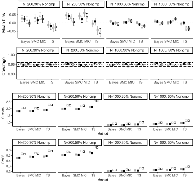
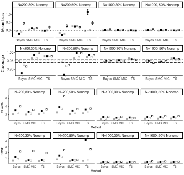
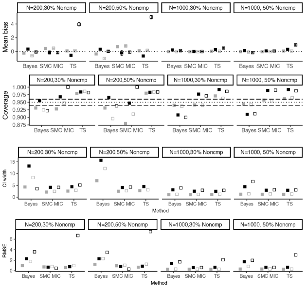
Figure 1 shows the mean bias (top) and CI coverage rate and width (middle) and RMSE (bottom) corresponding to scenarios with continuous outcome. Results for binary outcomes appear in Figure 2 (for ) and Figure 3 (for ).
With continuous outcome, all methods show close to zero bias, whether the true CACE is small or large, or the outcome is fully observed or partially missing. However, the bias is more pronounced with wider MCE CIs, that do not cross 0 in many settings with small sample size (). This bias is much reduced at the larger sample size, with MCE CIs that contain 0 in all settings with fully observed outcome when analysing with Bayesian or SMC MIC. TSLS exhibits some significant non-zero bias, especially where there are missing outcomes.
Coverage rates are close to the nominal value (between 94 and 96%). CI width is smaller for SMC MIC and Bayesian methods than TSLS, with SMC MIC slightly outperforming Bayesian methods in many scenarios. In terms of RMSE, we observe that both Bayesian and SMC MIC result in very similar values, inline with theoretical results about their equivalence. TSLS has a larger RMSE. These results support the claim that the SMC MIC method is more efficient than TSLS.
With binary outcomes, in scenarios where , Bayesian estimates are more varied, with some significant negative bias where the local odds ratio is large, and the sample size is small (the largest being 13% in absolute value). All bias becomes negligible at larger sample sizes (). The bias has implications for the coverage in the small sample scenarios, and Bayesian estimation results in low coverage (88%). Coverage is acceptable in most other settings. The bias is likely the result of the informative prior used for the log odds ratio, which puts more probability on smaller odds ratios values. In contrast, SMC MIC results in positive bias with small sample sizes, but appears unbiased in larger samples. With small samples it results in over coverage. At larger sample sizes, CI coverage rates is once again between 94% and 96%.
TSRI, which is expected to be consistent in these settings, results in small bias and valid CI coverage in scenarios where , but substantial bias (around 30%) is present when the true conditional local log odds ratio is large and the sample size small.
When comparing CI width and RMSE, we observed similar patterns to those exhibited with continuous outcomes, namely SMC MIC slightly outperforming Bayesian methods in many scenarios, which in turn outperforms TS methods.
In scenarios where , Figure 3 shows all methods report some bias with small sample sizes. The most extreme bias for Bayesian methods is negative 50%, while for SMC MIC is 40% (for both, this occurred where the true conditional CACE is small, there is 50% noncompliers and missing outcomes). However, both Bayesian and SMC MIC have nearly no bias when the sample size is . In contrast, TSRI reports considerable bias even at the larger sample size, 13% where and where , in line with the results of Cai et al. (2011).
Regarding coverage rates, Bayesian methods results in coverage above 90% in all settings. With the small sample size, SMC MIC results in under-coverage (88%) in one scenario (due to the considerable bias present. In contrast, where there is missing outcome data, it reports coverage rates close to 100%. Coverage is acceptable for the larger sample size though. TSRI reports coverage rates reasonably close to the nominal values but the CI width larger than after the other methods. In particular, where the CI width resulting from TSRI, with small sample size, missing outcome data and large true CACE is .
In terms of RMSE, in settings where the effect of compliance in the control group is small (), TSRI has smallest RMSE, despite reporting larger biases. In settings with larger effect of complying for the unexposed (), SMC MIC outperforms the other methods.
5 Motivating example: the COPERS trial
We now illustrate the methods in practice by applying each in turn to a real RCT. The COping with persistent Pain, Effectiveness Research in Self-management trial (COPERS) was a randomised controlled trial across 27 general practices and community services in the UK. It recruited 703 adults with musculoskeletal pain of at least three months duration, and randomised 403 participants to the active intervention and a further 300 to the control arm. The mean age of participants was 59.9 years, with 81% white, 67% female, 23% employed, 85% with pain for at least three years, and 23% on strong opioids.
Intervention participants were offered 24 sessions introducing them to cognitive behavioural (CB) approaches designed to promote self-management of chronic back pain. The sessions were delivered over three days within the same week with a follow-up session two weeks later. At the end of the three-day course, participants received a relaxation CD and self-help booklet. Controls received usual care and the same relaxation CD and self-help booklet. The control arm participants had no access to the active intervention sessions. Participants and group facilitators were not masked to the study arm they belonged to.
The primary outcome was pain-related disability at 12 months measured by the Chronic Pain Grade (CPG) disability sub-scale. This is a continuous measure on a scale from 0 to 100, with higher scores indicating worse pain-related disability. Secondary outcomes included depression (Hospital Anxiety and Depression Scale (HADS) depression sub-scale, ranging from 0 to 21) and social integration (Health Education Impact Questionnaire (HEIQ) social integration and support sub-scale, range 4–20), amongst others.
The ITT analysis found no evidence that the COPERS intervention had an effect on improving pain-related disability at 12 months (, % CI to ).
However, only 179 (45%) of those randomised to the active treatment attended all 24 sessions, with 322 (86.1%) receiving at least one session. Since poor attendance to the sessions was anticipated, the original statistical analysis plan included obtaining the CACE for primary and secondary outcomes, adjusted for all of the baseline covariates included in the primary analysis models, namely site of recruitment, age, gender and HADS depression score at baseline, and the corresponding outcome at baseline.
The original publication defined those attending at least half of the course (i.e. those present for at least 12 of the 24 course components) as the compliers, and used TSLS estimation after multiple imputation to estimate the CACE. It reported no evidence of a causal treatment effect on CPG disability at 12 months amongst the compliers ( , % CI to ). In contrast, there was evidence supporting a non-zero CACE for two secondary outcomes, depression and social integration (Taylor et al., 2016).
For this reason, we focus our re-analyses on these two outcomes. To exemplify the methods, HEIQ social integration at 12 months is considered as continuous, but HADS depression score is dichotomised by classifying those with a score of 11 and over as depressed, and not depressed otherwise (Bjelland et al., 2002). We analyse each outcome with a substantive model that adjusts for site of recruitment, age, gender and HADS depression score at baseline, and the corresponding outcome at baseline. In addition to these variables, our dataset also contains: Housing (Living arrangements: living alone versus living with others), whether they speak fluent English, ethnicity, employment (dichotomised as employed or in full time education versus not employed or in full-time education), age when left education (categorical), and the baseline measurements of other secondary outcomes, namely Pain Self-Efficacy Questionnaire (PSEQ), HADS anxiety score, and Chronic Pain Acceptance Questionnaire (CPAQ). Thirty-eight individuals (19 in each arm) originally recruited were completely lost to follow up, and are excluded from this analysis, as per the original COPERS analysis, leaving a sample size of 665 participants, who were followed up for 12 months, 384 allocated to active treatment, and 281 to the control (93% of those recruited).
Table 2 reports descriptive statistics and percentage of observations with missing data by treatment group. Geographical location (Warwick or London), age, gender, ethnicity, employment and educational attainment were all fully observed in the 665 participants.
We re-define treatment received, and consequently compliance, as taking any session in the intervention, in order to avoid more obvious exclusion restriction violations. For those participants completely unexposed to the training sessions, the exclusion restriction seems plausible, as it is unlikely that that random allocation has a direct effect, but since participants were not blinded to their allocation, we cannot completely rule out some psychological effects of knowing which group they belong to on depression and disability. The other two core IV assumptions, unconfoundedness and instrument relevance are justified by design, as is the monotonicity assumption, since the intervention was not available outside the trial.
We begin by performing a separate MI to analyse the ITT and the TSLS or TSRI respectively. We use MI by FCS to impute the outcome and the baseline variables with missing data (HADS depression and HEIQ social integration). We use employment, CPG disability, HADS anxiety and CPAQ as auxiliary variables (and HEIQ social integration at baseline for the HADS depression outcome). Since only employment was fully observed, all others also needed to be imputed. The Bayesian and SMC MIC methods deal with the missing data within the procedure, using the same auxiliary variables.
We report the ITT first, and then obtain a CACE with Bayesian, SMC MIC and two-stage methods in Table 3. As was the case in simulations, Bayesian and SMC MIC estimation methods resulted in very similar estimates, but SMC MIC reports shorter confidence intervals. In the case of continuous outcome, social integration, TSLS also reports a very similar point estimates, but with a larger SE.
For the binary outcome, HADS depression, we first notice that the point estimate obtained after TSRI is somewhat smaller in absolute value, so the treatment effect is less favourable. In addition the SE is considerably larger than that after either Bayesian or SMC MIC. As a result, we do not have a significant effect of treatment on the local log odds ratio of being depressed when receiving the COPERS intervention for the compliers, even though the point estimate is larger in absolute value than the ITT. Recall that TSRI requires that there is no effect of being a complier in the unexposed. It is very plausible that this assumption is violated in the COPERS trial, as the self-help booklet and relaxation CD may have a positive effect in reducing depression, in those that comply.
From this reanalysis, we conclude that there is a small positive causal effect of the COPERS intervention on improving social integration and reducing depression in those that comply by attending at least one session. These results depend on random allocation to treatment being a valid instrument, which as discussed previously seems a reasonable assumption. The local causal effects found are very small, and possibly not clinically relevant. This may be the result of our very low “dose” definition of compliance, which is however necessary to avoid violations of the exclusion restriction.
6 Discussion
This paper proposes the use of SMC MI of latent compliance classes to estimate the CACE using fully parametric mixture models fitted by maximum likelihood, and combined via Rubin’s rules. We have demonstrated empirically through simulations that the SMC MIC estimation has good finite sample performance, which is approximately equal to Bayesian estimation, and compares favourably to two-stage methods especially for estimating causal odds ratios.
The efficiency gains (in terms of SEs and narrower CIs) are more pronounced when auxiliary variables are incorporated. This is easily done within SMI MIC, because MI separates the imputation and the analysis stages, making it possible to estimate marginal local effects, i.e. only conditional on compliance class and treatment received. This is especially important for local odds ratios, given their non-collapsibility. Moreover, we have shown that for the estimation of local odds ratio, two-stage methods are only valid with certain modifications, for example by including the residuals from the first stage into the second stage and then again only in some special cases, namely where there is no effect of complying on the unexposed. While Bayesian estimation of the mixture models is valid, it is sensitive to the choice of priors, especially in small sample settings, and inclusion of several auxiliary variables requires careful coding, and the use of specialist software, making SMC MIC preferable to use in practical applications.
Taylor and Zhou (2009) previously proposed using MI for imputing the compliance classes in settings with missing outcomes, and compared MI estimation to existing Bayesian and frequentist methods. However, this work used a made-to-measure sampler, thus limiting its use in practice. In contrast, our method uses MI procedures already available in widely used statistical software packages (R and Stata). Another difference of our contribution is the focus on estimation where the estimand of interest for a binary outcome is the local causal odds ratios.
While the methods were exemplified and tested in the context of estimating the LATE in RCTs with non-adherence, binary exposure and binary compliance classes, assuming no always-takers and no defiers, SMI MIC is easily applicable to settings with always-takers, by simply using an multinomial imputation model for the compliance class, already implemented in the smcfcs packages. Also, although we assumed the strong exclusion restriction, it is possible to relax this, so that it only needs to hold for either the always-takers or the never-takers (Hirano et al., 2000). As our analysis of the illustrative example shows, the models can easily be modified to include baseline covariates (Little and Yau, 1998; Hirano et al., 2000). Moreover, this makes it possible to apply these methods to situations where the IV assumptions are only satisfied after conditioning on other variables, thus extending the applicability to certain observational settings where conditional IVs are more plausible.
The present study has some limitations. We have focused on the LATE estimand, which is often criticised because the estimates obtained apply to a stratum of the population (the compliers) which cannot be observed in practice, thus limiting its applicability. However, the LATE may provide some useful information about the average causal effect in the entire population. See Baiocchi (Baiocchi et al., 2014) for a discussion on this. Moreover, the average treatment effect on the compliers may be of interest in its own right, and patients are interested in this being estimated and reported, especially when they expect to comply with the treatment (Murray et al., 2018). In such cases, it may be desirable to describe the compliers, by modelling their distribution in terms of observed characteristics (Brookhart et al., 2006; Angrist and Pischke, 2008).
All methods considered here assume a specific parametric model and as such the estimates are sensitive to these parametric assumptions (Tan, 2006). In addition, we consider only situations where the identification assumptions hold. There are several options to study the sensitivity to departures from these assumptions. For example, if the exclusion restriction does not hold, a Bayesian parametric model can use priors on the non-zero direct effect of randomisation on the outcome for identification (Conley et al., 2012). Since these models are only weakly identified, the results depend strongly on the prior distributions. Alternatively, violations of the exclusion restriction can also be handled by using baseline covariates to model the probability of compliance directly, within structural equation modelling via expectation maximisation (Jo, 2002b, a).
Settings where the instrument is only weakly correlated with the exposure have not been considered here. Nevertheless, Bayesian methods have been shown to perform better than TS methods when the instrument is weak (Burgess and Thompson, 2012). Weak instruments may result in larger biases, which may be present due to model misspecification. Since the methods presented are not robust to such misspecifications, this is a particular concern. This suggest a possible extension to the work presented here, where more flexible non-parametric MI could be of use.
Extending our proposal to hierarchical settings, for example for cluster randomised trials with non-compliance, where the mixture models include a random effect for clustering, should be straightforward, as the compliance classes in these models can be imputed in a substantive model compatible manner by using the newly developed SMC functionality of the multilevel MI R package JOMO (Quartagno and Carpenter, 2018). However, careful consideration of the assumptions in the presence of (partial) interference at the cluster level is required (Sobel, 2006). Future research directions could include exploiting the additional flexibility of SMC MIC and extend our method to handle time-varying non-compliance in longitudinal settings.
In summary, our results show that SMC MIC provides a practical inferentially reliable method for estimation of the local average treatment effects, even when the target estimand is a causal odds ratio, and in the presence of missing outcome data.
Acknowledgements
The authors thank Prof. Stephanie Taylor and the COPERS trial team for access to the data.
Karla DiazOrdaz is supported by UK Medical Research Council Skills Development Fellowship MR/L011964/1. James Carpenter is supported by the Medical Research Council, grant numbers MC UU 12023/21 and MC UU 12023/29.
Supplementary Materials
References
- Angrist and Pischke (2008) Angrist, J. and Pischke, J. (2008). Mostly Harmless Econometrics: An Empiricist’s Companion. Princeton University Press.
- Angrist and Imbens (1995) Angrist, J. D. and Imbens, G. W. (1995). Two-stage least squares estimation of average causal effects in models with variable treatment intensity. Journal of the American statistical Association 90, 431–442.
- Angrist et al. (1996) Angrist, J. D., Imbens, G. W., and Rubin, D. B. (1996). Identification of causal effects using instrumental variables. Journal of the American Statistical Association 91, pp. 444–455.
- Baiocchi et al. (2014) Baiocchi, M., Cheng, J., and Small, D. S. (2014). Instrumental variable methods for causal inference. Statistics in Medicine 33, 2297–2340.
- Bartlett et al. (2014) Bartlett, J. W., Seaman, S. R., White, I. R., and Carpenter, J. R. (2014). Multiple imputation of covariates by fully conditional specification: Accommodating the substantive model. Statistical Methods in Medical Research epub, epub.
- Bjelland et al. (2002) Bjelland, I., Dahl, A. A., Haug, T. T., and Neckelmann, D. (2002). The validity of the hospital anxiety and depression scale: an updated literature review. Journal of psychosomatic research 52, 69–77.
- Brookhart et al. (2006) Brookhart, M. A., Wang, P., Solomon, D. H., and Schneeweiss, S. (2006). Evaluating short-term drug effects using a physician-specific prescribing preference as an instrumental variable. Epidemiology (Cambridge, Mass.) 17, 268.
- Burgess et al. (2015) Burgess, S., Small, D. S., and Thompson, S. G. (2015). A review of instrumental variable estimators for mendelian randomization. Statistical Methods in Medical Research .
- Burgess and Thompson (2012) Burgess, S. and Thompson, S. G. (2012). Improving bias and coverage in instrumental variable analysis with weak instruments for continuous and binary outcomes. Statistics in Medicine 31, 1582–1600.
- Cai et al. (2011) Cai, B., Small, D. S., and Have, T. R. T. (2011). Two-stage instrumental variable methods for estimating the causal odds ratio: Analysis of bias. Statistics in Medicine 30, 1809–1824.
- Clarke and Windmeijer (2012) Clarke, P. S. and Windmeijer, F. (2012). Instrumental variable estimators for binary outcomes. Journal of the American Statistical Association 107, 1638–1652.
- Collins et al. (2001) Collins, L. M., Schafer, J. L., and Kam, C. (2001). A comparison of inclusive and restrictive strategies in modern missing data procedures. Psychological Methods 6, 330–351.
- Conley et al. (2012) Conley, T. G., Hansen, C. B., and Rossi, P. E. (2012). Plausibly exogenous. Review of Economics and Statistics 94(1), 260–272.
- Didelez et al. (2010) Didelez, V., Meng, S., and Sheehan, N. A. (2010). Assumptions of iv methods for observational epidemiology. Statistical Science 25, 22–40.
- Dodd et al. (2012) Dodd, S., White, I., and Williamson, P. (2012). Nonadherence to treatment protocol in published randomised controlled trials: a review. Trials 13, 84.
- Frangakis and Rubin (2002) Frangakis, C. E. and Rubin, D. B. (2002). Principal stratification in causal inference. Biometrics 58, 21–29.
- Gelman et al. (2008) Gelman, A., Jakulin, A., Pittau, M. G., and Su, Y.-S. (2008). A weakly informative default prior distribution for logistic and other regression models. Ann. Appl. Stat. 2, 1360–1383.
- Hirano et al. (2000) Hirano, K., Imbens, G. W., Rubin, D. B., and Zhou, X.-H. (2000). Assessing the effect of an influenza vaccine in an encouragement design. Biostatistics 1, 69–88.
- Imbens (2001) Imbens, G. (2001). Comment on: "estimation of limited-dependent variable models with dummy endogenous regressors: Simple strategies for empirical practice’, by joshua angrist. Journal of Business and Economic Statistics 19, 17–20.
- Imbens and Angrist (1994) Imbens, G. W. and Angrist, J. D. (1994). Identification and estimation of local average treatment effects. Econometrica 62, 467–475.
- Imbens and Rubin (1997) Imbens, G. W. and Rubin, D. B. (1997). Bayesian inference for causal effects in randomized experiments with noncompliance. The Annals of Statistics 25, 305–327.
- Jo (2002a) Jo, B. (2002a). Estimation of intervention effects with noncompliance: Alternative model specifications. Journal of Educational and Behavioral Statistics 27, 385–409.
- Jo (2002b) Jo, B. (2002b). Model misspecification sensitivity analysis in estimating causal effects of interventions with non-compliance. Statistics in Medicine 21, 3161–3181.
- Jo and Muthén (2001) Jo, B. and Muthén, B. O. (2001). Modeling of intervention effects with noncompliance: A latent variable approach for randomized trials. New developments and techniques in structural equation modeling pages 57–87.
- Little and Yau (1998) Little, R. J. and Yau, L. H. (1998). Statistical techniques for analyzing data from prevention trials: Treatment of no-shows using rubin’s causal model. Psychological Methods 3, 147.
- Liu et al. (2013) Liu, J., Gelman, A., Hill, J., Su, Y. S., and Kropko, J. (2013). On the stationary distribution of iterative imputations. Biometrika 101, 155–173.
- Murray et al. (2018) Murray, E. J., Caniglia, E. C., Swanson, S. A., Hernández-Díaz, S., and Hernán, M. A. (2018). Patients and investigators prefer measures of absolute risk in subgroups for pragmatic randomized trials. Journal of Clinical Epidemiology 103, 10 – 21.
- Palmer et al. (2008) Palmer, T. M., Thompson, J. R., Tobin, M. D., Sheehan, N. A., and Burton, P. R. (2008). Adjusting for bias and unmeasured confounding in mendelian randomization studies with binary responses. International Journal of Epidemiology 37, 1161–1168.
- Quartagno and Carpenter (2018) Quartagno, M. and Carpenter, J. (2018). jomo: A package for Multilevel Joint Modelling Multiple Imputation.
- Rubin (1987) Rubin, D. B. (1987). Multiple imputation for nonresponse in surveys. New York: Wiley.
- Seaman et al. (2012) Seaman, S. R., Bartlett, J. W., and White, I. R. (2012). Multiple imputation of missing covariates with non-linear effects and interactions: an evaluation of statistical methods. BMC medical research methodology 12, 46.
- Sobel (2006) Sobel, M. E. (2006). What do randomized studies of housing mobility demonstrate? causal inference in the face of interference. Journal of the American Statistical Association 101, 1398–1407.
- Tan (2006) Tan, Z. (2006). Regression and weighting methods for causal inference using instrumental variables. Journal of the American Statistical Association 101, 1607–1618.
- Taylor and Zhou (2009) Taylor, L. and Zhou, X. H. (2009). Multiple imputation methods for treatment noncompliance and nonresponse in randomized clinical trials. Biometrics 65, 88–95.
- Taylor et al. (2016) Taylor, S. J., Carnes, D., and Homer, Kate, e. a. (2016). Improving the self-management of chronic pain: Coping with persistent pain, effectiveness research in self-management (copers). Programme Grants for Applied Research 4,.
- Terza (2014) Terza, J. V. (2014). Simpler standard errors for multi-stage regression-based estimators: Illustrations in health economics. In Keynote Address, Mexican Stata Users Group Meeting, Mexico City.
- Terza et al. (2008) Terza, J. V., Basu, A., and Rathouz, P. J. (2008). Two-stage residual inclusion estimation: Addressing endogeneity in health econometric modeling. Journal of Health Economics 27, 531 – 543.
- Vansteelandt et al. (2011) Vansteelandt, S., Bowden, J., Babanezhad, M., Goetghebeur, E., et al. (2011). On instrumental variables estimation of causal odds ratios. Statistical Science 26, 403–422.
- White (2005) White, I. R. (2005). Uses and limitations of randomization-based efficacy estimators. Statistical Methods in Medical Research 14, 327–347.
- White et al. (2010) White, I. R., Daniel, R., and Royston, P. (2010). Avoiding bias due to perfect prediction in multiple imputation of incomplete categorical variables. Computational statistics & data analysis 54, 2267–2275.
- Wooldridge (2010) Wooldridge, J. M. (2010). Econometric Analysis of Cross Section and Panel Data. MIT Press.
- Yau and Little (2001) Yau, L. H. and Little, R. J. (2001). Inference for the complier-average causal effect from longitudinal data subject to noncompliance and missing data, with application to a job training assessment for the unemployed. Journal of the American Statistical Association 96, 1232–1244.
- Yucel and Dermitas (2010) Yucel, R. and Dermitas, H. (2010). Impact of non-normal random effects on inference by multiple imputation: A simulation assessment. Comput Stat Data Anal 54, 790–801.
| Factor | Levels | |
|---|---|---|
| sample size | 200 | 1000 |
| percentage of compliers | 70 | 50 |
| type of outcome | Continuous | Binary |
| conditional true CACE in the link scale | ||
| causal effect of complying on the unexposeda | ||
| missing outcome | no | MAR given |
| a only for binary outcome scenarios | ||
| Control | Intervention | |
|---|---|---|
| N analysed (N=665) | ||
| N (%) Switched | ||
| Fully observed Baseline variables | ||
| age | ||
| Mean (SD) | ||
| gender | ||
| Male (%) | ||
| site of recruitment | ||
| Warwick (%) | ||
| Employment | ||
| full time (%) | ||
| Baseline variables with missing data | ||
| CPG disability | ||
| N (%) missing | ||
| Observed Mean (SD) | ||
| HEIQ social integration | ||
| N (%) missing | ||
| Observed Mean (SD) | ||
| HADS depression score | ||
| N (%) missing | ||
| Observed Mean (SD) | ||
| HADS anxiety | ||
| N (%) missing | ||
| Observed Mean (SD) | ||
| Outcomes at 12 months | ||
| HEIQ social integration | ||
| N (%) missing | ||
| Observed Mean (SD) | ||
| HADS depression score | ||
| N (%) missing | ||
| Observed Mean (SD) |
| Method | CACE | SE | 95% CI |
|---|---|---|---|
| HEIQ social integration | |||
| ITT | |||
| Bayesian | |||
| SMC MIC | |||
| TSLS | |||
| HADS depression | (log-odds ratio scale) | ||
| ITT | |||
| Bayesian | |||
| SMC MIC | |||
| TSRI |