Chiral symmetry breaking corrections to the pseudoscalar pole contribution of the Hadronic Light-by-Light piece of $a_{\mu}$

Abstract:

We have studied the $P\to\gamma^{\star}\gamma^{\star}$ form factor in Resonance Chiral Theory, with $P=\pi^{0}\eta\eta^{\prime}$, to compute the contribution of the pseudoscalar pole to the hadronic light-by-light piece of the anomalous magnetic moment of the muon. In this work we allow the leading $U(3)$ chiral symmetry breaking terms, obtaining the most general expression for the form factor up to $\mathcal{O}(m_{P}^{2})$. The parameters of the Effective Field Theory are obtained by means of short distance constraints on the form factor and matching with the expected behavior from QCD. Those parameters that cannot be fixed in this way are fitted to experimental determinations of the form factor within the spacelike region. Chiral symmetry relations among the transition form factors for $\pi^{0},\eta$ and $\eta^{\prime}$ allow for a simultaneous fit to experimental data for the three mesons. This shows an inconsistency between the BaBar $\pi^{0}$ data and the rest of the experimental inputs. Thus, we find a total pseudoscalar pole contribution of $a_{\mu}^{P,HLbL}=(8.47\pm 0.16)\cdot 10^{-10}$ for our best fit (that neglecting the BaBar $\pi^{0}$ data). Also, a preliminary rough estimate of the impact of NLO in $1/N_{C}$ corrections and higher vector multiplets (asym) enlarges the uncertainty up to $a_{\mu}^{P,HLbL}=(8.47\pm 0.16_{\rm stat}\pm 0.09_{N_{C}}{}^{+0.5}_{-0.0_{\rm asym}})10^{-10}$. This contribution is based on our work in ref. [1].

1 Introduction

The intrinsic magnetic moment of particles is an outstanding observable, thanks to the first measurement of the magnetic moment of silver atoms in Stern-Gerlach experiments, the non-commutative nature of angular momentum was made evident. Also, it helped us realize there is an intrinsic angular momentum associated to each fundamental particle, known as spin. This was a crucial discovery for the description of fundamental particles through the development of Quantum Field Theory and their electromagnetic interactions by means of Quantum Electrodynamics (QED).

The magnetic moment of a particle is defined to be the coupling strength between its electromagnetic current and a magnetic field. As a result of this, one finds that the magnetic moment must be proportional to the angular momentum of the particle. One can compute the intrinsic magnetic moment for fundamental particles that couple to the electromagnetic field calculating their interaction with a classic electromagnetic field (as done by Dirac [2]). This approach gives an intrinsic magnetic moment

$$\mu=g\frac{q}{2m}s,$$ (1)

where $q$ is the electric charge, $m$ is the mass of the particle, $s$ is the spin and $g=2$ is the gyromagnetic factor. A precise measurement done by Isidor Isaac Rabi’s group [3] showed a deviation from the value given by Dirac. This was explained by Julian Schwinger who computed the quantum correction to the interaction strength between the electromagnetic current and the magnetic field, leading him to develop the necessary tools to renormalize QED in order to calculate the NLO correction [4], $\delta\mu/\mu=\alpha/\pi+\mathcal{O}\left[(\alpha/\pi)^{2}\right]$, eliminating the incompatibility. The quantum corrections to $g=2$ define the anomalous magnetic moment

$$a=\frac{g-2}{2}.$$ (2)

Ever since, the anomalous magnetic moment of the electron, $a_{e}$, has been measured in evermore precise ways, demanding more precise theoretical determinations of it.

On the other hand, if one is interested in the search for Beyond Standard Model (BSM) effects in this observable one has to take into account that dimension six operators will be proportional to the fermion mass divided by heavy BSM scales. Since any observable depends on the squared modulus of the amplitude, such BSM effects will give considerably larger contributions on heavier particles. Being that the muon is $\sim 200$ times heavier than the electron, BSM effects will yield a higher signal in $a_{\mu}$ than in $a_{e}$. These effects would be even higher in the $\tau$ lepton, however $a_{\tau}$ is still compatible with zero [7]. Hence, the study of intrinsic magnetic moment of fundamental particles is still a very interesting subject nowadays.

The current experimental value [7] of $a_{\mu}=(11\hskip 4.30554pt659\hskip 4.30554pt209.1\pm 6.3)\cdot 10^{-10}$, has been compared with very precise theoretical predictions. These can be devided in three main parts, namely the QED part which contains contributions mainly from virtual leptons and their electromagnetic interactions up to order $\left(\alpha/\pi\right)^{5}$ [8]. This is the main contribution to the total $a_{\mu}$. Nevertheless, its uncertainty, ${\Delta a_{\mu}}_{\rm QED}=0.008\cdot 10^{-10}$, is three orders of magnitude smaller than the experimental one. The second is the electroweak contribution which accounts for electroweak interactions excluding those which are pure electromagnetic interactions. The computation of these up to two loops gives an uncertainty ${\Delta a_{\mu}}_{\rm EW}=0.10\cdot 10^{-10}$ [7], which is still very small compared to the experimental one.

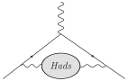
Figure 1: Hadronic contributions to $a_{\mu}$. The diagram on the left-hand-side represents all contributions from the hadronic vacuum to the self energy of the virtual photon, called Hadronic Vacuum Polarization (HVP). The diagram on the right-hand-side represents all contributions from elastic scattering of two photons, called Hadronic Light-by-Light scattering (HLbL).

The remaining contributions are those containing quarks and strong interactions, these are separated into two parts, the Hadronic Vacuum Polarization (HVP) and the Hadronic Light-by-Light scattering (HLbL), given in figure 1. The former can be extracted completely from experimental data on $R_{\rm had}=\sigma(e^{+}e^{-}\to{\rm hadrons})/\sigma(e^{+}e^{-}\to\mu^{+}\mu^{-})$ and contributes with an uncertainty ${\Delta a_{\mu}}_{\rm HVP}=3.4\cdot 10^{-10}$ [7]; the latter cannot be fully obtained from experimental observables and needs to be obtained either numerically or on a model dependent basis. However, this contributes with an error ${\Delta a_{\mu}}_{\rm HLbL}=2.6\cdot 10^{-10}$ [7]. These uncertainties are of the same order of magnitude as that given by the experiment. The most interesting fact is that the theoretical prediction is smaller than the measured $a_{\mu}$, having an incompatibility of $\sim 3.5\sigma$. This has motivated new experiments aiming to increase the precision in the determination of $a_{\mu}$, reducing the experimental error by, at least, a factor 4 in both, E34 at J-PARC [13] and muon g-2 at Fermilab [14]. Therefore, an effort must be done in the theoretical part to reduce the uncertainty by a similar factor. Since the HLbL part cannot be, nowadays, completely obtained from experiment, a deeper analysis of this part is necessary in order to reduce its uncertainty.

This work is focused on the main contribution to the HLbL piece of the anomalous magnetic moment of the muon, $a_{\mu}^{HLbL}$, which is given by the pseudoscalar exchange between pairs of photons, $a_{\mu}^{P,HLbL}$, [15] as shown in figure 2. All that is needed to compute such contributions to $a_{\mu}$ is the Transition Form Factor (TFF), $\mathcal{F}_{P\gamma^{\star}\gamma^{\star}}(q^{2},p^{2})$, of the pseudoscalar mesons coupling to two off-shell photons with virtualities $q^{2}$ and $p^{2}$. As has been shown in ref [16], $a_{\mu}^{P,HLbL}$ is almost fully determined by contributions at Euclidian squared photon momenta $-q^{2},-p^{2}\lesssim 1$ GeV². Therefore, it will be dominated mainly by the lowest-lying resonant part of the TFF and higher energies effects will give very small contributions. To describe the pseudoscalar-TFF we rely on the extension of $\chi$PT [17] which incorporates the lightest resonances in a chiral invariant way [18], namely Resonance Chiral Theory (R$\chi$T). Instead of using the complete basis of operators for resonances [19], we will rely on the more simple basis given in [20] to model vector meson interactions with pseudo-Goldstone bosons, since both are equivalent for describing vertices involving only one pseudo-Goldstone [21]; nevertheless, we will use [19] to account for pseudoscalar resonances effects. The novelty in our approach is that we account for all the leading order terms that break explicitly chiral symmetry, which enter as corrections in powers of the squared pseudo-Goldstone bosons masses, $m_{P}^{2}$.

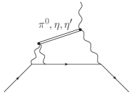
Figure 2: Main contribution to the Hadronic Light-by-Light piece of $a_{\mu}$.

2 Flavour $U(3)$ breaking

In this section, we will not show the full basis of operators ([17, 18, 19, 20, 22, 23, 24]), but will only show those which bring about the $U(3)$ breaking terms; the complete description is given in [1]. To consistently include all terms which break $U(3)$, an $\mathcal{O}(p^{6})$ odd-intrinsic R$\chi$T Lagrangian with no resonances must be considered. The contributions of $\mathcal{O}(p^{4})$ will be given by the Wess-Zumino-Witten functional [22]. The relevant non-resonant operators of $\mathcal{O}(p^{6})$ are

$${O}_{7}^{W} = i\epsilon_{\mu\nu\alpha\beta}\langle\chi_{-}f_{+}^{\mu\nu}f_{+}^{\alpha\beta}\rangle,$$

$${O}_{8}^{W} = i\epsilon_{\mu\nu\alpha\beta}\langle\chi_{-}\rangle\,\langle f_{+}^{\mu\nu}f_{+}^{\alpha\beta}\rangle,$$

$${O}_{22}^{W} = i\epsilon_{\mu\nu\alpha\beta}\langle u^{\mu}\{\nabla_{\rho}f_{+}^{\rho\nu},f_{+}^{\alpha\beta}\}\rangle.$$ (3)

A correction to the vector resonance-photon coupling will be given by the interaction

$$\mathcal{L}_{VJ}=\frac{\lambda_{V}}{\sqrt{2}}\langle V_{\mu\nu}\{f^{\mu\nu}_{+},\chi_{+}\}\rangle.$$ (4)

There is also a correction to the mass of the vector resonances from V-V interactions

$$\mathcal{L}_{VV}=-e_{m}^{V}\{V_{\mu\nu}V^{\mu\nu}\chi_{+}\}.$$ (5)

As a result, the masses of the vector resonances are given by

$$M_{\rho}^{2}=M_{\omega}^{2}=M_{V}^{2}-4e_{m}^{V}m_{\pi}^{2},\hskip 43.05542ptM_{\phi}^{2}=M_{V}^{2}-4e_{m}^{V}\Delta_{2K\pi}^{2},$$ (6)

where $\Delta_{2K\pi}^{2}=2m_{K}^{2}-m_{\pi}^{2}$ and $M_{V}$ is the mass associated with the vector nonet in the chiral and large $N_{C}$ limits.

3 Transition Form Factor

The Transition Form Factor (TFF) is defined through the $P\to\gamma^{\star}\gamma^{\star}$ decay amplitude, where the dressing of the photons comes from the interaction with resonances and pseudo-Goldstones through their respective operators

$$\mathcal{M}_{P\to\gamma^{\star}\gamma^{\star}}=ie^{2}\varepsilon^{\mu\nu\alpha\beta}{q_{1}}_{\mu}{q_{2}}_{\nu}{\epsilon_{1}^{*}}_{\alpha}{\epsilon_{2}^{*}}_{\beta}\mathcal{F}_{P\gamma^{\star}\gamma^{\star}}(q_{1}^{2},q_{2}^{2}),$$ (7)

where $\epsilon_{i}=\epsilon(q_{i})$ is the polarization of the photon with momentum $q_{i}$. Here, Bose symmetry implies $\mathcal{F}_{P\gamma^{\star}\gamma^{\star}}(q_{1}^{2},q_{2}^{2})=\mathcal{F}_{P\gamma^{\star}\gamma^{\star}}(q_{2}^{2},q_{1}^{2})$. One can impose relations among the parameters of the model by demanding that the TFF exhibits the short-distance behaviour expected from QCD [25, 26],

$$\lim_{q^{2}\to\infty}\mathcal{F}_{P\gamma^{\star}\gamma^{\star}}(q^{2},q^{2})=\mathcal{O}(q^{-2}){\rm\quad\quad and\quad\quad}\lim_{q^{2}\to\infty}\mathcal{F}_{P\gamma\gamma^{\star}}(0,q^{2})=\mathcal{O}(q^{-2}).$$ (8)

The full list of constraints obtained in this way for the parameters are shown in ref [1]. After applying the relations among parameters, the simplified expression of the TFF for $\pi^{0}$ reads

$$\mathcal{F}_{\pi\gamma^{\star}\gamma^{\star}}(q_{1}^{2},q_{2}^{2})=\frac{32\pi^{2}m_{\pi}^{2}F_{V}^{2}d_{123}^{\star}-N_{C}M_{V}^{2}M_{\rho}^{2}}{12\pi^{2}F_{\pi}D_{\rho}(q_{1}^{2})D_{\rho}(q_{2}^{2})},$$ (9)

where $F_{\pi}$ is the $\pi$ decay constant, $D_{R}(q^{2})=M_{R}^{2}-q^{2}$ is the denominator of the propagator of the vector-meson resonance $R$, with the resonance masses $M_{R}$ given by (6), and $d_{123}^{\star}$ is a free parameter. Analogously, the simplified expression for the TFF of the $\eta$ is given by

$$\mathcal{F}_{\eta\gamma^{\star}\gamma^{\star}}(q_{1}^{2},q_{2}^{2}) = \frac{1}{12\pi^{2}FD_{\rho}(q_{1}^{2})D_{\rho}(q_{2}^{2})D_{\phi}(q_{1}^{2})D_{\phi}(q_{2}^{2})}\times$$

$$\left\{-\frac{N_{C}M_{V}^{2}}{3}\left[5C_{q}M_{\rho}^{2}D_{\phi}(q_{1}^{2})D_{\phi}(q_{2}^{2})-\sqrt{2}C_{s}M_{\phi}^{2}D_{\rho}(q_{1}^{2})D_{\rho}(q_{2}^{2})\right]\right.$$

$$+\frac{32\pi^{2}F_{V}^{2}d_{123}^{\star}m_{\eta}^{2}}{3}\left[(5C_{q}D_{\phi}(q_{1}^{2})D_{\phi}(q_{2}^{2})-\sqrt{2}C_{s}D_{\rho}(q_{1}^{2})D_{\rho}(q_{2}^{2})\right]$$

$$\left.-\frac{256\pi^{2}F_{V}^{2}d_{2}^{\star}}{3}\left[(5C_{q}\Delta_{\eta\pi}^{2}D_{\phi}(q_{1}^{2})D_{\phi}(q_{2}^{2})+\sqrt{2}C_{s}\Delta_{2K\pi\eta}^{2}D_{\rho}(q_{1}^{2})D_{\rho}(q_{2}^{2})\right]\right\},$$

where $d_{2}^{\star}$ is a free parameter, $\Delta_{\eta\pi}^{2}=m_{\eta}^{2}-m_{\pi}^{2}$, $\Delta_{2K\pi\eta}^{2}=2m_{K}^{2}-m_{\pi}^{2}-m_{\eta}^{2}$ and $C_{q/s}$ are the $\eta-\eta^{\prime}$ mixing parameters. The TFF for the $\eta^{\prime}$ can be obtained from this by the substitutions $m_{\eta}\to m_{\eta^{\prime}}$, $C_{q}\to C_{q}^{\prime}$ and $C_{s}\to-C_{s}^{\prime}$.

As said previously, the evaluation of the contribution from the pseudo-Goldstone exchange is obtained by using the integral expressions given in ref. [16] substituting the TFF for each contribution. To get to these expressions, one has to assume that the form factor can be expressed in the following way

$$\mathcal{F}_{P\gamma^{\star}\gamma^{\star}}(q_{1}^{2},q_{2}^{2})=\frac{F}{3}\left[f(q^{2})+\sum_{V_{i}}\frac{1}{M_{V_{i}}^{2}-q_{2}^{2}}g_{V_{i}}(q_{1}^{2})\right].$$ (11)

After applying the short distance constraints, the function $f(q^{2})$ vanishes for all the form factors, in accordance with previous determinations of such function [16, 27].

Since some of the parameters could not be constrained by imposing the correct high-energy behavior of the TFF, we fit them to experimental determinations excluding the time-like ($q^{2}>0$) region of photon four-momenta, since radiative corrections might give large contributions to the TFF in such region [28]. We fitted simultaneously the parameters of our TFF of the $\pi^{0}$, $\eta$ and $\eta^{\prime}$ mesons to the decay widths of the three pseudo-Goldstones given by [7], also to the singly off-shell TFF from CELLO [29] and CELLO [30] for the three pseudo-Goldstones, LEP for $\eta^{\prime}$ [31], BaBar for $\pi^{0}$ [32], BaBar for $\eta$ and $\eta^{\prime}$ [33] and Belle for $\pi^{0}$ [34]. All further details on the fit are given in ref [1].

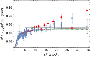
Figure 3: Fitted spacelike $\pi^{0}$-TFF. The red region shows the TFF using all data within 1-$\sigma$ and the green region is the one excluding the BaBar data. The red diamonds are the BaBar data [32].

The fit including all data (fit1) gave a total $\chi^{2}/dof=150./101$. In comparison, the fit neglecting only the BaBar $\pi^{0}$ data from the whole set (fit 2), gave an improved value of $\chi^{2}/dof=69./84$, which we regarded as our best fit. The $\pi^{0}$-TFF prediction for both fits are shown in Fig. 3, where $Q^{2}=-q^{2}$ is the Euclidean squared momentum.

4 Pseudo-Goldstone pole contribution to $a_{\mu}^{HLbL}$

4.1 Meson exchange prediction with one vector resonance multiplet

The contribution from the pseudo-Goldstone pole to the HLbL piece of $a_{\mu}$, $a_{\mu}^{P,HLbL}$, is obtained using the integral representation given in [16]. The total pseudo-Goldstone contribution is estimated using a Monte Carlo run with $5\cdot 10^{3}$ events which randomly generates the eight fit parameters with a normal distribution according to their mean values, errors and correlations. The contributions from the three pseudo-Goldstones are integrated at the same time, accounting in this way for the correlation between the three contributions. Thus we obtain

$$a_{\mu}^{P,HLbL}=(8.47\pm 0.16)\cdot 10^{-10}.$$ (12)

The prediction using the set of parameters from fit 1 is $a_{\mu}^{P,HLbL}=(8.58\pm 0.16)\cdot 10^{-10}$, which despite a higher central value is completely compatible with the value we obtain using the parameters of fit 2. This is expected since one can see from Figure 3 that the absolute value of the form factor is larger for this set of parameters at large $Q_{i}^{2}=-q_{i}^{2}$; however, since the integration kernels are dominated by the region for $Q_{i}^{2}\lesssim 1$ GeV² (as said above), the compatibility among both values is expected.

We also study $a_{\mu}^{P,HLbL}$ by taking chiral and large $N_{C}$ limits of the TFF, keeping the physical masses in the integration kernels, giving $(F/F_{\pi})^{2}a_{\mu}^{P,LbL}=8.27\cdot 10^{-10}$. This is obtained with the central values of the parameters of our best fit in these limits. Comparing the latter with the central value of our contribution and taking $F\approx F_{\pi}$, we see that the chiral corrections account for a $\sim 2.5$% (up to corrections in $F/F_{\pi}$). This suggests that further chiral corrections (NNLO), suppressed by additional powers of $m_{P}^{2}$, must be negligible.

4.2 Further error analysis

The NLO effects in the $1/N_{C}$ expansion can be estimated by including the effects of the off-shell width in the $\rho$ meson propagator. The NLO contributions to the latter are accounted mainly by the $\pi\pi$ and $\overline{K}K$ loops, the expression for such corrections reads [35]

$$M_{\rho}^{2}-q^{2}\quad\to\quad M_{\rho}^{2}-q^{2}+\frac{q^{2}M_{\rho}^{2}}{96\pi^{2}F_{\pi}^{2}}\left(A_{\pi}(q^{2})+\frac{1}{2}A_{K}(q^{2})\right),$$ (13)

where the loop functions are given by

$$A_{P}(q^{2})=\log\frac{m_{P}^{2}}{M_{\rho}^{2}}+8\frac{m_{P}^{2}}{q^{2}}-\frac{5}{3}+\sigma_{P}^{3}(q^{2})\log\left(\frac{\sigma_{P}(q^{2})+1}{\sigma_{P}(q^{2})-1}\right),$$ (14)

being $\sigma_{P}(s)=\sqrt{1-\frac{4m_{P}^{2}}{s}}$. It is worth to notice that the loop functions are real for $q^{2}<4m_{P}^{2}$, so that the propagator is real in the whole spacelike ($q^{2}<0$) region of photon momenta, where it is integrated. Since now the propagator of the $\rho$ meson is not a rational function of $q^{2}$, it cannot be expressed as in eq. (11). Therefore, in order to be able to express the TFF in such form we approximate the form factor by imposing the condition obtained above that $f(q^{2})$ vanishes and making the substitution (13) in the rest of the expression in eq. (11). This allows us to represent the TFF in such way that one can use the integral representation in [16] to obtain the $a_{\mu}^{P,HLbL}$ contribution. Thus, we obtain ${a_{\mu}^{P,HLbL}|}_{\text{LO+NLO}}-{a_{\mu}^{P,HLbL}|}_{\text{LO}}=-0.09\cdot 10^{-10}$.

This is, nonetheless, just one of the possible NLO corrections in $1/N_{C}$ to the anomalous magnetic moment. One-loop modifications to the $\pi^{0}VV^{\prime}$ vertex can be, e.g., equally important in the space-like domain and may lead to a positive con tribution to $a_{\mu}^{P,HLbL}$. Thus, we take the absolute value of this shift as a crude estimate of the $1/N_{C}$ effects:

$$\left(\Delta a_{\mu}^{P,HLbL}\right)_{1/N_{C}}=\pm 0.09\cdot 10^{-10}.$$ (15)

From the expressions (9) and (3) it is evident that our TFF does not fulfill the exact short distance QCD limit expected for $Q_{1}^{2}=Q_{2}^{2}=Q^{2}$ when $Q^{2}\to\infty$ [25, 26]. Our form factors underestimate the real contribution since they behave as $1/Q^{4}$ instead than $1/Q^{2}$ near this limit. One rough estimate can be given by computing the total contribution to $a_{\mu}^{P,HLbL}$ with the form factors in the chiral limit with one and two vector resonance multiplets and comparing both results. The complete details of such procedure are given in [1]. Thus, we obtain

$$\left(\Delta a_{\mu}^{P,HLbL}\right)_{\text{asym}}=^{+0.5}_{-0.0}\cdot 10^{-10}.$$ (16)

5 Conclusions

We have given a more accurate description of the TFF within the framework of R$\chi$T, including terms up to order $m_{P}^{2}$ for the first time in a chiral invariant Lagrangian approach. This led to a more precise computation of the contribution from the $P$-pole to $a_{\mu}$. By looking at the difference of our results with that using the TFF in the chiral limit ($0.20\cdot 10^{-10}$) it seems that further chiral corrections will be negligible. Considering all possible contributions to the error, we get

$$a_{\mu}^{P,HLbL}=(8.47\pm 0.16_{\text{stat}}\pm 0.09_{1/N_{C}}{{}^{+0.5}_{-0.0}}_{\text{asym}})\cdot 10^{-10},$$ (17)

where the first error (stat) comes from the fit, the second from possible $1/N_{C}$ corrections and the last due to the wrong asymptotic (asym) behavior of our TFF estimated through the effect of heavier vector resonances.

- [1] A. Guevara, P. Roig and J. J. Sanz-Cillero, JHEP 1806 (2018) 160.
- [2] P. A. M. Dirac, Proc. Roy. Soc. Lond. A 118 (1928) 351. doi:10.1098/rspa.1928.0056.
- [3] J. E. Nafe, E. B. Nelson and I. I. Rabi, Phys. Rev. 71 (1947) 914.
- [4] J. S. Schwinger, Phys. Rev. 73 (1948) 416.
- [5] Joan Ruiz Vidal, Talk given at Xth CPAN days, Salamaca, Spain. Available at https://indico.ific.uv.es/event/3366/contributions/9868/attachments/6640/
- [6] E. Bagli et al., Eur. Phys. J. C 77 (2017) no.2, 71.
- [7] C. Patrignani et al., Particle Data Group collab., Chin. Phys. C 40 (2016) 100001.
- [8] T. Kinoshita and M. Nio, Phys. Rev. D 73 (2006) 053007.
- [9] G. Colangelo, M. Hoferichter, M. Procura and P. Stoffer, JHEP 1409 (2014) 091; G. Colangelo, M. Hoferichter, B. Kubis, M. Procura and P. Stoffer, Phys. Lett. B 738 (2014) 6; G. Colangelo, M. Hoferichter, M. Procura and P. Stoffer, JHEP 1509 (2015) 074; Phys. Rev. Lett. 118 (2017) no.23, 232001; JHEP 1704 (2017) 161.
- [10] M. Hoferichter, B. L. Hoid, B. Kubis, S. Leupold and S. P. Schneider, Phys. Rev. Lett. 121 (2018) no.11, 112002; JHEP 1810 (2018) 141.
- [11] V. Pauk and M. Vanderhaeghen, Phys. Rev. D 90 (2014) no.11, 113012; A. Nyffeler, Phys. Rev. D 94 (2016) no.5, 053006; I. Danilkin and M. Vanderhaeghen, Phys. Rev. D 95 (2017) no.1, 014019; F. Hagelstein and V. Pascalutsa, Phys. Rev. Lett. 120 (2018) no.7, 072002.
- [12] R. Parker, C. Yu, W. Zhong, B. Estey and H. Müller, Science 360 (2018) 191-195
- [13] H. Iinuma, H. Nakayama, K. Oide, K. i. Sasaki, N. Saito, T. Mibe and M. Abe, Nucl. Instrum. Meth. A 832 (2016) 51.
- [14] W. Gohn, arXiv:1801.00084 [hep-ex].
- [15] F. Jegerlehner and A. Nyffeler, Phys. Rept. 477 (2009) 1.
- [16] M. Knecht and A. Nyffeler, Phys. Rev. D 65 (2002) 073034.
- [17] S. Weinberg, Physica A 96 (1979) 327; J. Gasser and H. Leutwyler, Annals Phys. 158 (1984) 142; Nucl. Phys. B 250 (1985) 465.
- [18] G. Ecker, J. Gasser, A. Pich, E. De Rafael, Nucl. Phys. B321 (1989) 311; G. Ecker, J. Gasser, H. Leutwyler, A. Pich, E. De Rafael, Phys. Lett. B223 (1989) 425.
- [19] K. Kampf and J. Novotny, Phys. Rev. D 84 (2011) 014036.
- [20] P. D. Ruiz-Femenia, A. Pich and J. Portoles, JHEP 0307 (2003) 003.
- [21] P. Roig and J. J. Sanz Cillero, Phys. Lett. B 733 (2014) 158.
- [22] J. Wess and B. Zumino, Phys. Lett. 37B (1971) 95; E. Witten, Nucl. Phys. B223 (1983) 422.
- [23] J. Bijnens, L. Girlanda and P. Talavera, Eur. Phys. J. C 23 (2002) 539.
- [24] V. Cirigliano, et al.,Nucl. Phys. B 753 (2006) 139.
- [25] S. J. Brodsky and G. R. Farrar, Phys. Rev. Lett. 31 (1973) 1153.
- [26] G. P. Lepage and S. J. Brodsky, Phys. Rev. D 22 (1980) 2157.
- [27] P. Roig, A. Guevara and G. López Castro, Phys. Rev. D 89 (2014) no.7, 073016.
- [28] T. Husek, K. Kampf, S. Leupold and J. Novotny, Phys. Rev. D 97 (2018) no.9, 096013.
- [29] H. J. Behrend et al. [CELLO Collaboration], Z. Phys. C 49 (1991) 401.
- [30] J. Gronberg et al. [CLEO Collaboration], Phys. Rev. D 57 (1998) 33.
- [31] M. Acciarri et al. [L3 Collaboration], Phys. Lett. B 418 (1998) 399.
- [32] B. Aubert et al. [BaBar Collaboration], Phys. Rev. D 80 (2009) 052002.
- [33] P. del Amo Sanchez et al. [BaBar Collaboration], Phys. Rev. D 84 (2011) 052001.
- [34] S. Uehara et al. [Belle Collaboration], Phys. Rev. D 86 (2012) 092007.
- [35] D. Gomez Dumm, A. Pich and J. Portoles, Phys. Rev. D 62 (2000) 054014.