Protection Against Reconstruction and Its Applications in Private Federated Learning

Abstract

In large-scale statistical learning, data collection and model fitting are moving increasingly toward peripheral devices—phones, watches, fitness trackers—away from centralized data collection. Concomitant with this rise in decentralized data are increasing challenges of maintaining privacy while allowing enough information to fit accurate, useful statistical models. This motivates local notions of privacy—most significantly, local differential privacy, which provides strong protections against sensitive data disclosures—where data is obfuscated before a statistician or learner can even observe it, providing strong protections to individuals’ data. Yet local privacy as traditionally employed may prove too stringent for practical use, especially in modern high-dimensional statistical and machine learning problems. Consequently, we revisit the types of disclosures and adversaries against which we provide protections, considering adversaries with limited prior information and ensuring that with high probability, ensuring they cannot reconstruct an individual’s data within useful tolerances. By reconceptualizing these protections, we allow more useful data release—large privacy parameters in local differential privacy—and we design new (minimax) optimal locally differentially private mechanisms for statistical learning problems for all privacy levels. We thus present practicable approaches to large-scale locally private model training that were previously impossible, showing theoretically and empirically that we can fit large-scale image classification and language models with little degradation in utility.

1 Introduction

New, more powerful computational hardware and access to substantial amounts of data has made fitting accurate models for image classification, text translation, physical particle prediction, astronomical observation, and other predictive tasks possible with previously infeasible accuracy [7, 2, 49]. In many modern applications, data comes from measurements on small-scale devices with limited computation and communication ability—remote sensors, phones, fitness monitors—making fitting large scale predictive models both computationally and statistically challenging. Moreover, as more modes of data collection and computing move to peripherals—watches, power-metering, internet-enabled home devices, even lightbulbs—issues of privacy become ever more salient.

Such large-scale data collection motivates substantial work. Stochastic gradient methods are now the de facto approach to large-scale model-fitting [70, 15, 60, 29], and recent work of McMahan et al. [54] describes systems (which they term federated learning) for aggregating multiple stochastic model-updates from distributed mobile devices. Yet even if only updates to a model are transmitted, leaving all user or participant data on user-owned devices, it is easy to compromise the privacy of users [37, 56]. To see why this issue arises, consider any generalized linear model based on a data vector $x$, target $y$, and with loss of the form $\ell(\theta;x,y)=\phi(\langle\theta,x\rangle,y)$. Then $\nabla_{\theta}\ell(\theta;x,y)=c\cdot x$ for some $c\in\mathbb{R}$, a scalar multiple of the user’s clear data $x$—a clear compromise of privacy. In this paper, we describe an approach to fitting such large-scale models both privately and practically.

A natural approach to addressing the risk of information disclosure is to use differential privacy [35], in which one defines a mechanism $M$, a randomized mapping from a sample $\boldsymbol{x}$ of data points to some space $\mathcal{Z}$, which is $\varepsilon$-differentially private if

$$\frac{\mathbb{P}(M(\boldsymbol{x})\in S)}{\mathbb{P}(M(\boldsymbol{x}^{\prime})\in S)}\leq e^{\varepsilon}$$ (1)

for all samples $\boldsymbol{x}$ and $\boldsymbol{x}^{\prime}$ differing in at most one entry. Because of its strength and protection properties, differential privacy and its variants are the standard privacy definition in data analysis and machine learning [19, 32, 22]. Nonetheless, implementing such an algorithm presumes a level of trust between users and a centralized data analyst, which may be undesirable or even untenable, as the data analyst has essentially unfettered access to a user’s data. Another approach to protecting individual updates is to use secure multiparty computation (SMC), sometimes in conjunction with differential privacy protections [14]. Traditional approaches to SMC require substantial communication and computation, making them untenable for large-scale data collection schemes, and Bonawitz et al. [14] address a number of these, though individual user communication and computation still increases with the number of users submitting updates and requires multiple rounds of communication, which may be unrealistic when estimating models from peripheral devices.

An alternative to these approaches is to use locally private algorithms [67, 36, 31], in which an individual keeps his or her data private even from the data collector. Such scenarios are natural in distributed (or federated) learning scenarios, where individuals provide data from their devices [53, 3] but wish to maintain privacy. In our learning context, where a user has data $x\in\mathcal{X}$ that he or she wishes to remain private, a randomized mechanism $M:\mathcal{X}\to\mathcal{Z}$ is $\varepsilon$-local differentially private if for all $x,x^{\prime}\in\mathcal{X}$ and sets $S\subset\mathcal{Z}$,

$$\frac{\mathbb{P}(M(x)\in S)}{\mathbb{P}(M(x^{\prime})\in S)}\leq e^{\varepsilon}.$$ (2)

Roughly, a mechanism satisfying inequality (2) guarantees that even if an adversary knows that the initial data is one of $x$ or $x^{\prime}$, the adversary cannot distinguish them given an outcome $Z$ (the probability of error must be at least $1/(1+e^{\varepsilon})$) [68]. Taking as motivation this testing definition, the “typical” recommendation for the parameter $\varepsilon$ is to take $\varepsilon$ as a small constant [68, 35, 32].

Local privacy protections provide numerous benefits: they allow easier compliance with regulatory strictures, reduce risks (such as hacking) associated with maintaining private data, and allow more transparent protection of user privacy, because unprotected private data never leaves an individual’s device. Yet substantial work in the statistics, machine learning, and computer science communities has shown that local differential privacy and its relaxations cause nontrivial challenges for learning systems. Indeed, Duchi, Jordan, and Wainwright [30, 31] and Duchi and Rogers [26] show that in a minimax (worst case population distribution) sense, learning with local differential privacy must suffer a degradation in sample complexity that scales as $d/\min\{\varepsilon,\varepsilon^{2}\}$, where $d$ is the dimension of the problem; taking $\varepsilon$ as a small constant here suggests that estimation in problems of even moderate dimension will be challenging. Duchi and Ruan [27] develop a complementary approach, arguing that a worst-case analysis is too conservative and may not accurately reflect the difficulty of problem instances one actually encounters, so that an instance-specific theory of optimality is necessary. In spite of this instance-specific optimality theory for locally private procedures—that is, fundamental limits on learning that apply to the particular problem at hand—Duchi and Ruan’s results suggest that local notions of privacy as currently conceptualized restrict some of the deployments of learning systems.

We consider an alternative conceptualization of privacy protections and the concomitant guarantees from differential privacy and the likelihood ratio bound (2). The testing interpretation of differential privacy suggests that when $\varepsilon\gg 1$, the definition (2) is almost vacuous. We argue that, at least in large-scale learning scenarios, this testing interpretation is unrealistic, and allowing mechanisms with $\varepsilon\gg 1$ may provide satisfactory privacy protections, especially when there are multiple layers of protection. Rather than providing protections against arbitrary inferences, we wish to provide protection against accurate reconstruction of an individual’s data $x$. In the large scale learning scenarios we consider, an adversary given a random observation $x$ likely has little prior information about $x$, so that protecting only against reconstructing (functions of) $x$ under some assumptions on the adversary’s prior knowledge allows substantially improved model-fitting.

Our formal setting is as follows. For a parameter space $\Theta\subset\mathbb{R}^{d}$ and loss $\ell:\Theta\times\mathcal{X}\to\mathbb{R}_{+}$, we wish to solve the risk minimization problem

$$\mathop{\rm minimize}_{\theta\in\Theta}~{}L(\theta):=\mathbb{E}[\ell(\theta,X)].$$ (3)

The standard approach [40] to such problems is to construct the empirical risk minimizer $\widehat{\theta}_{n}=\mathop{\rm argmin}_{\theta}\frac{1}{n}\sum_{i=1}^{n}\ell(\theta,X_{i})$ for data $X_{i}\stackrel{{\scriptstyle\rm iid}}{{\sim}}P$, the distribution defining the expectation (3). In this paper, however, we consider the stochastic minimization problem (3) while providing both local privacy to individual data $X_{i}$ and—to maintain the satisfying guarantees of centralized differential privacy (1)—stronger guarantees on the global privacy of the output $\widehat{\theta}_{n}$ of our procedure. With this as motivation, we describe our contributions at a high level. As above, we argue that large local privacy (2) parameters, $\varepsilon\gg 1$, still provide reasonable privacy protections. We develop new mechanisms and privacy protecting schemes that more carefully reflect the statistical aspects of problem (3); we demonstrate that these mechanisms are minimax optimal for all ranges of $\varepsilon\in[0,d]$, a broader range than all prior work (where $d$ is problem dimension). A substantial portion of this work is devoted to providing practical procedures while providing meaningful local privacy guarantees, which currently do not exist. Consequently, we provide extensive empirical results that demonstrate the tradeoffs between private federated (distributed) learning scenarios, showing that it is possible to achieve performance comparable to federated learning procedures without privacy safeguards.

1.1 Our approach and results

We propose and investigate a two-pronged approach to model fitting under local privacy. Motivated by the difficulties associated with local differential privacy we discuss in the immediately subsequent section, we reconsider the threat models (or types of disclosure) in locally private learning. Instead of considering an adversary with access to all data, we consider “curious” onlookers, who wish to decode individuals’ data but have little prior information on them. Formalizing this (as we discuss in Section 2) allows us to consider substantially relaxed values for the privacy parameter $\varepsilon$, sometimes even scaling with the dimension of the problem, while still providing protection. While this brings us away from the standard guarantees of differential privacy, we can still provide privacy guarantees for the type of onlookers we consider.

This privacy model is natural in distributed model-fitting (federated learning) scenarios [53, 3]. By providing protections against curious onlookers, a company can protect its users against reconstruction of their data by, for example, internal employees; by encapsulating this more relaxed local privacy model within a broader central differential privacy layer, we can still provide satisfactory privacy guarantees to users, protecting them against strong external adversaries as well.

We make several contributions to achieve these goals. In Section 2, we describe a model for curious adversaries, with appropriate privacy guarantees, and demonstrate how (for these curious adversaries) it is still nearly impossible to accurately reconstruct individuals’ data. We then detail a prototypical private federated learning system in Section 3. In this direction, we develop new (minimax optimal) privacy mechanisms for privatization of high-dimensional vectors in unit balls (Section 4). These mechanisms yield substantial improvements over the schemes Duchi et al. [31, 30] develop, which are optimal only in the case $\varepsilon\leq 1$, providing order of magnitude improvements over classical noise addition schemes, and we provide a unifying theorem showing the asymptotic behavior of a stochastic-gradient-based private learning scheme in Section 4.4. As a consequence of this result, we conclude that we have (minimax) optimal procedures for many statistical learning problems for all privacy parameters $\varepsilon\leq d$, the dimension of the problem, rather than just $\varepsilon\in[0,1]$. We conclude our development in Section 5 with several large-scale distributed model-fitting problems, showing how the tradeoffs we make allow for practical procedures. Our approaches allow substantially improved model-fitting and prediction schemes; in situations where local differential privacy with smaller privacy parameter fails to learn a model at all, we can achieve models with performance near non-private schemes.

1.2 Why local privacy makes model fitting challenging

To motivate our approaches, we discuss why local privacy causes some difficulties in a classical learning problem. Duchi and Ruan [27] help to elucidate the precise reasons for the difficulty of estimation under $\varepsilon$-local differential privacy, and we can summarize them heuristically here, focusing on the machine learning applications of interest. To do so, we begin with a brief detour through classical statistical learning and the usual convergence guarantees that are (asymptotically) possible [66].

Consider the population risk minimization problem (3), and let $\theta^{\star}=\mathop{\rm argmin}_{\theta}L(\theta)$ denote its minimizer. We perform a heuristic Taylor expansion to understand the difference between $\widehat{\theta}_{n}$ and $\theta^{\star}$. Indeed, we have

$$0=\frac{1}{n}\sum_{i=1}^{n}\nabla\ell(\widehat{\theta}_{n},X_{i}) =\frac{1}{n}\sum_{i=1}^{n}\nabla\ell(\theta^{\star},X_{i})+\frac{1}{n}\sum_{i=1}^{n}(\nabla^{2}\ell(\theta^{\star},X_{i})+\mbox{error}_{i})(\widehat{\theta}_{n}-\theta^{\star})$$

$$=\frac{1}{n}\sum_{i=1}^{n}\nabla\ell(\theta^{\star},X_{i})+(\nabla^{2}L(\theta^{\star})+o_{P}(1))(\widehat{\theta}_{n}-\theta^{\star}),$$

(for $\mbox{error}_{i}$ an error term in the Taylor expansion of $\ell$), which—when carried out rigorously—implies

$$\widehat{\theta}_{n}-\theta^{\star}=\frac{1}{n}\sum_{i=1}^{n}\underbrace{-\nabla^{2}L(\theta^{\star})^{-1}\nabla\ell(\theta^{\star};X_{i})}_{=:\psi(X_{i})}+o_{P}(1/\sqrt{n}).$$ (4)

The influence function $\psi$ [66] of the parameter $\theta$ measures the effect that changing a single observation $X_{i}$ has on the resulting estimator $\widehat{\theta}_{n}$.

All (regular) statistically efficient estimators asymptotically have the form (4) [66, Ch. 8.9], and typically a problem is “easy” when the variance of the function $\psi(X_{i})$ is small—thus, individual observations do not change the estimator substantially. In the case of local differential privacy, however, as Duchi and Ruan [27] demonstrate, (optimal) locally private estimators typically have the form

$$\widehat{\theta}_{n}-\theta^{\star}=\frac{1}{n}\sum_{i=1}^{n}\left[\psi(X_{i})+W_{i}\right]$$ (5)

where $W_{i}$ is a noise term that must be taken so that $\psi(x)$ and $\psi(x^{\prime})$ are indistinguishable for all $x,x^{\prime}$. Essentially, a local differentially private procedure cannot leave $\psi(x)$ small even when it is typically small (i.e. the problem is easy) because it could be large for some value $x$. In locally private procedures, this means that differentially private tools for typically “insensitive” quantities (cf. [32]) cannot apply, as an individual term $\psi(X_{i})$ in the sum (5) is (obviously) sensitive to arbitrary changes in $X_{i}$. An alternative perspective comes via information-theoretic ideas [26]: differential privacy constraints are essentially equivalent to limiting the bits of information it is possible to communicate about individual data $X_{i}$, where privacy level $\varepsilon$ corresponds to a communication limit of $\varepsilon$ bits, so that we expect to lose in efficiency over non-private or non-communication-limited estimators at a rate roughly of $d/\varepsilon$ (see Duchi and Rogers [26] for a formalism). The consequences of this are striking, and extend even to weakenings of local differential privacy [26, 27]: adaptivity to easy problems is essentially impossible for standard $\varepsilon$-locally-differentially private procedures, at least when $\varepsilon$ is small, and there must be substantial dimension-dependent penalties in the error $\widehat{\theta}_{n}-\theta^{\star}$. Thus, to enable high-quality estimates for quantities of interest in machine learning tasks, we explore locally differentially private settings with larger privacy parameter $\varepsilon$.

2 Privacy protections

In developing any statistical machine learning system providing privacy protections, it is important to consider the types of attacks that we wish to protect against. In distributed model fitting and federated learning scenarios, we consider two potential attackers: the first is a curious onlooker who can observe all updates to a model and communication from individual devices, and the second is from a powerful external adversary who can observe the final (shared) model or other information about individuals who may participate in data collection and model-fitting. For the latter adversary, essentially the only effective protection is to use a small privacy parameter in a localized or centralized differentially private scheme [54, 35, 59]. For the curious onlookers, however—for example, internal employees of a company fitting large-scale models—we argue that protecting against reconstruction is reasonable.

2.1 Differential privacy and its relaxations

We begin by discussing the various definitions of privacy we consider, covering both centralized and local definitions of privacy. We begin with the standard centralized definitions, which extend the basic differential privacy definition (1), and allow a trusted curator to view the entire dataset. We have

Definition 2.1 (Differential privacy, Dwork et al. [35, 34]).

A randomized mechanism $M:\mathcal{X}^{n}\to\mathcal{Z}$ is $(\varepsilon,\delta)$ differentially private if for all samples $\boldsymbol{x},\boldsymbol{x}^{\prime}\in\mathcal{X}^{n}$ differing in at most a single example, for all measurable sets $S\subset\mathcal{Z}$

$$\mathbb{P}(M(\boldsymbol{x})\in S)\leq e^{\varepsilon}\mathbb{P}(M(\boldsymbol{x}^{\prime})\in S)+\delta.$$

Other variants of privacy require that likelihood ratios are near one on average, and include concentrated and Rényi differential privacy [33, 18, 59]. Recall that the Rényi $\alpha$-divergence between distributions $P$ and $Q$ is

$$D_{\alpha}\left({P}|\!|{Q}\right):=\frac{1}{\alpha-1}\log\int\left(\frac{dP}{dQ}\right)^{\alpha}dQ,$$

where $D_{\alpha}\left({P}|\!|{Q}\right)=D_{\rm kl}\left({P}|\!|{Q}\right)$ when $\alpha=1$ by taking a limit. We abuse notation, and for random variables $X$ and $Y$ distributed as $P$ and $Q$, respectively, write $D_{\alpha}\left({X}|\!|{Y}\right):=D_{\alpha}\left({P}|\!|{Q}\right)$, which allows us to make the following

Definition 2.2 (Rényi-differential privacy [59]).

A randomized mechanism $M:\mathcal{X}^{n}\to\mathcal{Z}$ is $(\varepsilon,\alpha)$-Rényi differentially private if for all samples $\boldsymbol{x},\boldsymbol{x}^{\prime}\in\mathcal{X}^{n}$ differing in at most a single example,

$$D_{\alpha}\left({M(\boldsymbol{x})}|\!|{M(\boldsymbol{x}^{\prime})}\right)\leq\varepsilon.$$

Mironov [59] shows that if $M$ is $\varepsilon$-differentially private, then for any $\alpha\geq 1$, it is $(\min\{\varepsilon,2\alpha\varepsilon^{2}\},\alpha)$-Rényi private, and conversely, if $M$ is $(\varepsilon,\alpha)$-Rényi private, it also satisfies $(\varepsilon+\frac{\log(1/\delta)}{\alpha-1},\delta)$-differential privacy for all $\delta\in[0,1]$.

We often use local notions of these definitions, as we consider protections for individual data providers without trusted curation; in this case, the mechanism $M$ applied to an individual data point $x$ is locally private if the Definition 2.1 or 2.2 holds with $M(\boldsymbol{x})$ and $M(\boldsymbol{x}^{\prime})$ replaced by $M(x)$ and $M(x^{\prime})$, where $x,x^{\prime}\in\mathcal{X}$ are arbitrary.

2.2 Reconstruction breaches

Abstractly, we work in a setting in which a user or study participant has data $X$ he or she wishes to keep private. Via some process, this data is transformed into a vector $W$—which may simply be an identity transformation, but $W$ may also be a gradient of the loss $\ell$ on the datum $X$ or other derived statistic. We then privatize $W$ via a randomized mapping $W\to Z$. An onlooker wishes to estimate some function $f(X)$ on the private data $X$. In most scenarios with a curious onlooker, if $X$ or $f(X)$ is suitably high-dimensional, the onlooker has limited prior information about $X$, so that relatively little obfuscation is required in the mapping from $W\to Z$.

As a motivating example, consider an image processing scenario. A user has an image $X$, where $W\in\mathbb{R}^{d}$ are wavelet coefficients of $X$ (in some prespecified wavelet basis) [52]; without loss of generality, we assume we normalize $W$ to have energy $\left\|{W}\right\|_{2}=1$. Let $f(X)$ be a low-dimensional version of $X$ (say, based on the first 1/8 of wavelet coefficients); then (at least intuitively) taking $Z$ to be a noisy version of $W$ such that $\left\|{Z-W}\right\|_{2}\gtrsim 1$—that is, noise on the scale of the energy $\left\|{W}\right\|_{2}$—should be sufficient to guarantee that the observer is unlikely to be able to reconstruct $f(X)$ to any reasonable accuracy. Moreover, a simple modification of the techniques of Hardt and Talwar [39] shows that for $W\sim\mathsf{Uni}(\mathbb{S}^{d-1})$, any $\varepsilon$-differentially private quantity $Z$ for $W$ satisfies $\mathbb{E}[\left\|{Z-W}\right\|_{2}]\gtrsim 1$ whenever $\varepsilon\leq d-\log 2$. That is, we might expect that in the definition (2) of local differential privacy, even very large $\varepsilon$ provide protections against reconstruction.

With this in mind, let us formalize a reconstruction breach in our scenario. Here, the onlooker (or adversary) has a prior $\pi$ on $X\in\mathcal{X}$, and there is a known (but randomized) mechanism $M:\mathcal{W}\to\mathcal{Z}$, $W\mapsto Z=M(W)$. We then have the following definition.

Definition 2.3 (Reconstruction breach).

Let $\pi$ be a prior on $\mathcal{X}$, and let $X,W,Z$ be generated with Markov structure $X\to W\to Z=M(W)$ for a mechanism $M$. Let $f:\mathcal{X}\to\mathbb{R}^{k}$ be the target of reconstruction and $L_{\rm rec}:\mathbb{R}^{k}\times\mathbb{R}^{k}\to\mathbb{R}_{+}$ be a loss function. Then an estimator $\widehat{v}:\mathcal{Z}\to\mathbb{R}^{k}$ provides an $(\alpha,p,f)$-reconstruction breach for the loss $L_{\rm rec}$ if there exists $z$ such that

$$\mathbb{P}\left(L_{\rm rec}(f(X),\widehat{v}(z))\leq\alpha\mid M(W)=z\right)>p.$$ (6)

If for every estimator $\widehat{v}:\mathcal{Z}\to\mathbb{R}^{k}$,

$$\sup_{z\in\mathcal{Z}}\mathbb{P}\left(L_{\rm rec}(f(X),\widehat{v}(z))\leq\alpha\mid M(W)=z\right)\leq p,$$

then the mechanism $M$ is $(\alpha,p,f)$-protected against reconstruction for the loss $L_{\rm rec}$.

Key to Definition 2.3 is that it applies uniformly across all possible observations $z$ of the mechanism $M$—there are no rare breaches of privacy. This requires somewhat stringent conditions on mechanisms and also disallows relaxed privacy definitions beyond differential privacy.

2.3 Protecting against reconstruction

We can now develop guarantees against reconstruction. The simple insight is that if an adversary has a diffuse prior on the data of interest $f(X)$—is a priori unlikely to be able to accurately reconstruct $f(X)$ given no information—the adversary remains unlikely to be able to reconstruct $f(X)$ given differentially private views of $X$ even for very large $\varepsilon$. Key to this is the question of how “diffuse” we might expect an adversary’s prior to be. We detail a few examples here, providing what we call best-practices recommendations for limiting information, and giving some strong heuristic calculations for reasonable prior information.

We begin with the simple claim that prior beliefs change little under differential privacy, which follows immediately from Bayes’ rule.

Lemma 2.1.

Let the mechanism $M$ be $\varepsilon$-differentially private and let $V=f(X)$ for a measurable function $f$. Then for any $\pi\in\mathcal{P}$ on $\mathcal{X}$ and measurable sets $A,A^{\prime}\subset f(\mathcal{X})$, the posterior distribution $\pi_{V}(\cdot\mid z)$ (for $z=M(X)$) satisfies

$$\frac{\pi_{V}(A\mid z,z)}{\pi_{V}(A^{\prime}\mid z,z)}\leq e^{\varepsilon}\frac{\pi_{V}(A)}{\pi_{V}(A^{\prime})}.$$

Based on Lemma 2.1, we can show the following result, which guarantees that difficulty of reconstruction of a signal is preserved under private mappings.

Lemma 2.2.

Assume that the prior $\pi_{0}$ on $X$ is such that for a tolerance $\alpha$, probability $p(\alpha)$, target function $f$, and loss $L_{\rm rec}$, we have

$$\mathbb{P}_{\pi_{0}}(L_{\rm rec}(f(X),v_{0})\leq\alpha)\leq p(\alpha)~{}~{}\mbox{for~{}all~{}fixed}~{}v_{0}.$$

If $M$ is $\varepsilon$-differentially private, then it is $(\alpha,e^{\varepsilon}\cdot p(\alpha),f)$-protected against reconstruction for $L_{\rm rec}$.

Proof    Lemma 2.1 immediately implies that for any estimator $\widehat{v}$ based on $Z=M(X)$, we have for any realized $z$ and $V=f(X)$

$$\mathbb{P}(L_{\rm rec}(V,\widehat{v}(z))\leq\alpha\mid Z=z) =\int\mathbbm{1}\left\{L_{\rm rec}(v,\widehat{v}(z))\leq\alpha\right\}d\pi_{V}(v\mid z)$$

$$\leq e^{\varepsilon}\int\mathbbm{1}\left\{L_{\rm rec}(v,\widehat{v}(z))\leq\alpha\right\}d\pi_{V}(v).$$

The final quantity is $e^{\varepsilon}\mathbb{P}(L_{\rm rec}(f(X),v_{0})\leq\alpha)\leq e^{\varepsilon}p(\alpha)$ for $v_{0}=\widehat{v}(z)$, as desired. ∎

Let us make these ideas a bit more concrete through two examples: one when it is reasonable to assume a diffuse prior, one for much more peaked priors.

2.3.1 Diffuse priors and reconstruction of linear functions

For a prior $\pi$ on $X$ and $f:\mathcal{X}\to C\subset\mathbb{R}^{k}$, where $C$ is a compact subset of $\mathbb{R}^{k}$, let $\pi_{f}$ be the push-forward (induced prior) on $f(X)$ and let $\pi_{0}$ be some base measure on $C$ (typically, this will be a uniform measure). Then for $\rho_{0}\in[0,\infty]$ define the set of plausible priors

$$\mathcal{P}_{f}(\rho_{0}):=\left\{\pi~{}\mbox{on}~{}X~{}\mbox{s.t.}~{}\log\frac{d\pi_{f}(v)}{d\pi_{0}(v)}\leq\rho_{0},~{}\mbox{for~{}}v\in C\right\}.$$ (7)

For example, consider an image processing situation, where we wish to protect against reconstruction even of low-frequency information, as this captures the basic content of an image. In this case, we consider an orthonormal matrix $A\in\mathbb{C}^{k\times d}$, $AA^{*}=I_{k}$, and an adversary wishing to reconstruct the normalized projection

$$f_{A}(x)=\frac{Ax}{\left\|{Ax}\right\|_{2}}=\frac{Au}{\left\|{Au}\right\|_{2}}~{}~{}\mbox{for~{}}u=x/\left\|{x}\right\|_{2}.$$ (8)

For example, $A$ may be the first $k$ rows of the Fourier transform matrix, or the first level of a wavelet hierarchy, so the adversary seeks low-frequency information about $x$. In either case, the “low-frequency” $Ax$ is enough to give a sense of the private data, and protecting against reconstruction is more challenging for small $k$.

In the particular orthogonal reconstruction case, we take the initial prior $\pi_{0}$ to be uniform on $\mathbb{S}^{k-1}$—a reasonable choice when considering low frequency information as above—and consider $\ell_{2}$ reconstruction with $L_{\rm rec}(u,v)=\left\|{u/\left\|{u}\right\|_{2}-v/\left\|{v}\right\|_{2}}\right\|_{2}$ (when $v\neq 0$, otherwise setting $L_{\rm rec}(u,v)=\sqrt{2}$). For $V$ uniform and $v_{0}\in\mathbb{S}^{k-1}$, we have $\mathbb{E}[\left\|{V-v_{0}}\right\|_{2}^{2}]=2$, so that thresholds of the form $\alpha=\sqrt{2-2a}$ with $a$ small are the most natural to consider in the reconstruction (6). We have the following proposition on reconstruction after a locally differentially private release.

Proposition 1.

Let $M$ be $\varepsilon$-locally differentially private (2) and $k\geq 4$. Let $f=f_{A}$ as in Eq. (8) and $\pi\in\mathcal{P}_{f}(\rho_{0})$ as in Eq. (7). Then for $a\in[0,1]$, $M$ is $(\sqrt{2-2a},p(a),f_{A})$-protected against reconstruction for

$$p(a)=\begin{cases}\exp\left(\varepsilon+\rho_{0}+\frac{k}{2}\cdot\log(1-a^{2})\right)&\mbox{if~{}}a\in[0,1/\sqrt{2}]\\ \exp\left(\varepsilon+\rho_{0}+\frac{k-1}{2}\cdot\log(1-a^{2})-\log(2a\sqrt{k})\right)&\mbox{if~{}}a\in[\sqrt{2/k},1].\end{cases}$$

Simplifying this slightly and rewriting, assuming the reconstruction $\widehat{v}$ takes values in $\mathbb{S}^{k-1}$, we have

$$\mathbb{P}(\left\|{f(X)-\widehat{v}(Z)}\right\|_{2}\leq\sqrt{2-2a}\mid Z=z)\leq\exp\left(-\frac{ka^{2}}{2}\right)\exp(\varepsilon+\rho_{0})$$

for $f(x)=Ax/\left\|{Ax}\right\|$ and $a\leq 1/\sqrt{2}$. That is, unless $\varepsilon$ or $\rho_{0}$ are of the order of $k$, the probability of obtaining reconstructions better than (nearly) random guessing is extremely low.

Proof    Let $Y\sim\mathsf{Uni}\left(\mathbb{S}^{k-1}\right)$ and $v_{0}\in\mathbb{S}^{k-1}$. We then have

$$\left\|{Y-v_{0}}\right\|_{2}^{2}=2\cdot\left(1-\langle Y,v_{0}\rangle\right).$$

We collect a number of standard facts on the uniform distribution on $\mathbb{S}^{k-1}$ in Appendix D, which we reference frequently. Lemma D.1 implies that for all $v_{0}\in\mathbb{S}^{k-1}$ and $a\in[0,1/\sqrt{2}]$ that

$$\mathbb{P}_{\pi_{\rm uni}}(\left\|{Y-v_{0}}\right\|_{2}<\sqrt{2-2a})=\mathbb{P}\left(\langle Y,v_{0}\rangle>a\right)\leq(1-a^{2})^{k/2}$$

Because $V=f_{A}(X)$ has prior $\pi_{V}$ such that $d\pi_{V}/d\pi_{\rm uni}\leq e^{\rho_{0}}$, we obtain

$$\mathbb{P}_{\pi_{V}}\left(\left\|{V-v_{0}}\right\|_{2}<\sqrt{2-2a}\right)\leq e^{\rho_{0}}\cdot\left(1-a^{2}\right)^{k/2}.$$

Then Lemma 2.2 gives the first result of the proposition.

When the desired accuracy is higher (i.e. $a\in[\sqrt{2/k},1]$), Lemma D.1 with our assumed ratio bound between $\pi_{V}$ and $\pi_{\rm uni}$ implies

$$\mathbb{P}_{\pi_{V}}(\left\|{V-v_{0}}\right\|_{2}\leq\sqrt{2-2a})\leq e^{\rho_{0}}\mathbb{P}_{\pi_{\rm uni}}(\left\|{Y-v_{0}}\right\|_{2}<\sqrt{2-2a})\leq e^{\rho_{0}}\frac{(1-a^{2})^{\frac{k-1}{2}}}{2a\sqrt{k}}.$$

Applying Lemma 2.2 completes the proof. ∎

2.3.2 Reconstruction protections against sparse data

When it is unreasonable to assume that an individual’s data is near uniform on a $d$-dimensional space, additional strategies are necessary to limit prior information. We now view an individual data provider as having multiple “items” that an adversary wishes to investigate. For example, in the setting of fitting a word model on mobile devices—to predict next words in text messages to use as suggestions when typing, for example—the items might consist of all pairs and triples of words the individual has typed. In this context, we combine two approaches:

1. An individual contributes data only if he/she has sufficiently many data points locally (for example, in our word prediction example, has sent sufficiently many messages)

2. An individual’s data must be diverse or sufficiently stratified (in the word prediction example, the individual sends many distinct messages).

As Lemma 2.2 makes clear, if $M$ is $\varepsilon$-differentially private and for any fixed $v\in\mathcal{Z}$ we have $\mathbb{P}(L_{\rm rec}(v,f(X))\leq a)\leq p_{0}$, then for all functions $\widehat{f}$,

$$\mathbb{P}(L_{\rm rec}(\widehat{f}(M(X)),f(X))\leq a)\leq e^{\varepsilon}p_{0}.$$ (9)

We consider an example of sampling a histogram—specifically thinking of sampling messages or related discrete data. We call the elements words in a dictionary of size $d$, indexed by $j=1,\ldots,d$. To stratify the data (approach (ii)), we treat a user’s data as a vector $x\in\mathcal{X}\in\{0,1\}^{d}$, where $x_{j}=0$ if the user has not used word $j$, otherwise $x_{j}=1$. We do not allow a user to participate until $x^{T}\mathbf{1}\geq m$ for a particular “mini batch” size $m$ (approach (i)). Now, let us discuss the prior probability of reconstructing a user’s vector $x$. We consider reconstruction via precision and recall. Let $v\in\{0,1\}^{d}$ denote a vector of predictions of the used words, where $v_{j}=1$ if we predict word $j$ is used. Then we define

$$\mathsf{precision}(x,v):=\frac{v^{T}x}{v^{T}\mathbf{1}}~{}~{}\mbox{and}~{}~{}\mathsf{recall}(x,v):=\frac{v^{T}x}{\mathbf{1}^{T}x},$$

that is, precision measures the fraction of predicted words that are correct, and recall the fraction of used words the adversary predicts correctly. We say that the signal $x$ has been reconstructed for some $p,r$ if $\mathsf{precision}(x,v)\geq p$ and $\mathsf{recall}(x,v)\geq r$. Let us bound the probability of each of these events under appropriate priors on the vector $X\in\{0,1\}^{d}$.

Using Zipfian models of text and discretely sampled data [21], a reasonable a priori model of the sequence $X$, when we assume that a user must draw at least $m$ elements, is that independently

$$\mathbb{P}(X_{j}=1)=\min\left\{\frac{m}{j},1\right\}.$$ (10)

With this model for a prior, we may bound the probability of achieving good precision or recall:

Lemma 2.3.

Let $\gamma\geq 2$ and assume the vector $X$ satisfies the Zipfian model (10). Assume that the vector $v\in\{0,1\}^{d}$ satisfies $v^{T}\mathbf{1}\geq\gamma m$. Then

$$\mathbb{P}(\mathsf{precision}(v,X)\geq p)\leq\exp\left(-\min\left\{\frac{\left({p\gamma-1-\log\gamma}\right)_{+}^{2}m}{2\log\gamma},\frac{3}{4}\left({p\gamma-1-\log\gamma}\right)_{+}m\right\}\right).$$

Conversely, assume that the vector $v\in\{0,1\}^{d}$ satisfies $v^{T}\mathbf{1}\geq\gamma m$, and define $\tau(r,d,m,\gamma):=r(1+\log\frac{d}{m+1})-1-\log\gamma$. Then

$$\mathbb{P}(\mathsf{recall}(v,X)\geq r)\leq\exp\left(-\min\left\{\frac{\left({\tau(r,d,m,\gamma)}\right)_{+}^{2}m}{4(1-r^{2})\log\frac{d}{m}},\frac{3}{4}\left({\tau(r,d,m,\gamma)}\right)_{+}m\right\}\right).$$

See Appendix A.1 for a proof.

Considering Lemma 2.3, we can make a few simplifications to see the (rough) beginning reconstruction guarantees we consider—with explicit calculations on a per-application basis. In particular, we see that for any fixed precision value $p$ and recall value $r$, we may take $\gamma=\frac{2}{p}\log\frac{1}{p}$ to obtain that as long as $r\log\frac{d}{m}\geq 2\log\frac{1}{p}$, then

$$\mathbb{P}\left(\mathsf{precision}(v,X)\geq p~{}\mbox{and}~{}\mathsf{recall}(v,X)\geq r\right)\leq\max\left\{\exp\left(-cm\log\frac{1}{p}\right),\exp\left(-cm\log\frac{d}{m}\right)\right\}=:p_{r,d,m}.$$

for a numerical constant $c>0$. Thus, we have the following protection guarantee.

Proposition 2.

Let the conditions of Lemma 2.3 hold. Define the reconstruction loss $L_{\rm rec}(v,X)$ to be $1$ if $\mathsf{precision}(v,X)\geq p$ and $\mathsf{recall}(v,x)\geq r$, 0 otherwise, where $r\log\frac{d}{m}\geq 2\log\frac{1}{p}$. Then if $M$ is $\varepsilon$-locally differentially private, $M$ is $(0,e^{\varepsilon}p_{r,d,m})$-protected against reconstruction.

Consequently, we make the following recommendation: in the case that signals are dictionary-like, a best practice is to aggregate together at least $m=d^{\rho}$ such signals, for some power $\rho$, and use (local) privacy budget $\varepsilon$ in differentially private mechanisms of at most $\varepsilon=cm$, where $c$ is a small (near 0) constant. We revisit this in the language modeling applications in the experiments.

3 Applications in federated learning

Our overall goal is to implement federated learning, where distributed units send private updates to a shared model to a centralized location. Recalling our population risk (3), basic distributed learning procedures (without privacy) iterate as follows [13, 24, 17]:

1. A centralized parameter $\theta$ is distributed among a batch of $b$ workers, each with a local sample $X_{i}$, $i=1,\ldots,b$.

2. Each worker computes an update $\Delta_{i}:=\theta_{i}-\theta$ to the model parameters.

3. The centralized procedure aggregates $\{\Delta_{i}\}_{i=1}^{b}$ into a global update $\Delta$ and updates $\theta\leftarrow\theta+\Delta$.

In the prototypical stochastic gradient method, $\Delta_{i}=-\eta\nabla\ell(\theta,X_{i})$ for some stepsize $\eta>0$ in step 2, and $\Delta=\frac{1}{b}\sum_{i=1}^{b}\Delta_{i}$ is the average of the stochastic gradients at each sample $X_{i}$ in step 3.

In our private distributed learning context, we elaborate steps 2 and 3 so that each provides privacy protections: in the local update step 2, we use locally private mechanisms to protect individuals’ private data $X_{i}$—satisfying Definition 2.3 on protection against reconstruction breaches. Then in the central aggregation step 3, we apply centralized differential privacy mechanisms to guarantee that any model $\theta$ communicated to users in the broadcast 1 is globally private. The overall feedback loop provides meaningful privacy guarantees, as a user’s data is never transmitted clearly to the centralized server, and strong centralized privacy guarantees mean that the final and intermediate parameters $\theta$ provide no sensitive disclosures.

3.1 A private distributed learning system

Let us more explicitly describe the implementation of a distributed learning system. The outline of our system is similar to the development of Duchi et al. [30, 31, Sec. 5.2] and the system that McMahan et al. [55] outline; we differ in that we allow more general updates and privatize individual users’ data before communication, as the centralized data aggregator may not be completely trusted.

The stochastic optimization proceeds as follows. The central aggregator maintains the global model parameter $\theta\in\mathbb{R}^{d}$, and in each iteration, chooses a random subset (mini-batch) $\mathcal{B}$ of expected size $qN$, where $q\in(0,1)$ is the subsampling rate and $N$ the total population size available. Each individual $i\in\mathcal{B}$ sampled then computes a local update, which we describe abstractly by a method Update that takes as input the local sample $\boldsymbol{x}_{i}=\{x_{i,1},\ldots,x_{i,m}\}$ and central parameter $\theta$, then

$$\theta_{i}\leftarrow\texttt{Update}\left(\boldsymbol{x}_{i},\theta\right).$$

Many updates are possible. Perhaps the most popular rule is to apply a gradient update, where from an initial model $\theta_{0}$ and for stepsize $\eta$ we apply

$$\texttt{Update}(\boldsymbol{x}_{i},\theta_{0}):=\theta_{0}-\eta\frac{1}{m}\sum_{j=1}^{m}\nabla\ell(\theta_{0},x_{i,j})=\mathop{\rm argmin}_{\theta}\left\{\frac{1}{m}\sum_{j=1}^{m}\langle\nabla\ell(\theta_{0},x_{i,j}),\theta-\theta_{0}\rangle+\frac{1}{2\eta}\left\|{\theta-\theta_{0}}\right\|_{2}^{2}\right\}.$$

An alternative is to stochastic proximal-point-type updates [6, 46, 43, 12, 23], which update

$$\texttt{Update}(\boldsymbol{x}_{i},\theta_{0}):=\mathop{\rm argmin}_{\theta}\left\{\frac{1}{m}\sum_{j=1}^{m}\ell(\theta,x_{i,j})+\frac{1}{2\eta_{i}}\left\|{\theta-\theta_{0}}\right\|_{2}^{2}\right\},$$ (11)

or their relaxations to use approximate models [6, 5].

After computing the local update $\theta_{i}$, we privatize the scaled local difference $\Delta_{i}:=\frac{1}{\eta}(\theta_{i}-\theta_{0})$, which is the (stochastic) gradient mapping for typical model-based updates [6, 5], as this scaling by stepsize enforces a consistent expected update magnitude. We let

$$\widehat{\Delta}_{i}=M(\Delta_{i})$$ (12)

where $M$ is a private mechanism, be an unbiased (private) view of $\Delta_{i}$, detailing mechanisms $M$ in Section 4. Given the privatized local updates $\{\widehat{\Delta}_{i}\}_{i\in\mathcal{B}}$, we project the update of each onto an $\ell_{2}$-ball of fixed radius $\rho$, so that for $\mathsf{proj}_{\rho}(v):=\min\{\rho/\left\|{v}\right\|_{2},1\}\cdot v$ we consider the averaged gradient mapping

$$\widehat{\Delta}\leftarrow\frac{\eta}{qN}\left(\sum_{i\in\mathcal{B}}\mathsf{proj}_{\rho}(\widehat{\Delta}_{i})+Z\right)~{}~{}~{}\mbox{and}~{}~{}~{}\theta^{(t+1)}=\theta^{(t)}+\widehat{\Delta}.$$ (13)

The projection operation $\mathsf{proj}_{\rho}$ limits the contribution of any individual update, while the vector $Z\sim\mathsf{N}(0,\sigma^{2})$ is Gaussian and provides a centralized privacy guarantee, where we describe $\sigma^{2}$ presently. In the case that the loss functions $\ell$ are Lipschitz—typically the case in statistical learning scenarios with classification, for example, logistic regression—the projection is unnecessary as long as the data vectors $x_{i}$ lie in a compact space.

It remains to discuss the global privacy guarantees we provide via the noise addition $Z$. For any individual $i$, we have $\frac{1}{qN}\|{\mathsf{proj}_{\rho}(\widehat{\Delta}_{i})}\|_{2}\leq\rho/(qN)$; thus we may use Abadi et al.’s “moments accountant” analysis [1], which reposes on Rényi-differential privacy (Def. 2.2). We first present an intuitive explanation; the precise parameter settings we explain in the experiments, which make the privacy guarantees as sharp as possible using computational evaluations of the privacy parameters [1]. First, if $Q$ denotes the distribution (13) of $\widehat{\Delta}$ and $Q_{0}$ denotes its distribution when we remove a fixed user $i_{0}$, then the Rényi-2-divergence between the two [1, Lemma 3] satisfies

$$D_{2}\left({Q}|\!|{Q_{0}}\right)\leq\log\left[1+\frac{q^{2}}{1-q}\left(\exp\Big{(}\frac{\|{\widehat{\Delta}_{i_{0}}}\|_{2}^{2}}{\sigma^{2}}-1\Big{)}\right)\right]\leq\frac{q^{2}}{1-q}\left(e^{\rho^{2}/\sigma^{2}}-1\right),$$

and the Rényi-$\alpha$-divergence is $D_{\alpha}\left({Q}|\!|{Q_{0}}\right)\leq\frac{\alpha(\alpha-1)q^{2}}{1-q}(e^{\rho^{2}/\sigma^{2}}-1)+O(q^{3}\alpha^{3}/\sigma^{3})$ for $\alpha\leq\sigma^{2}\log\frac{1}{q\sigma}$. Thus, letting $\varepsilon_{\alpha,\textup{tot}}$ denote the cumulative Rényi-$\alpha$ privacy loss after $T$ iterations of the update (13), we have

$$\varepsilon_{\alpha,\textup{tot}}\leq T\frac{q^{2}}{1-q}\left[\exp\left(\frac{\rho^{2}}{\sigma^{2}}\right)-1\right]+O\left(\frac{q^{3}\alpha^{3}}{\sigma^{3}}\right).$$

This remains below a fixed $\varepsilon$ for

$$\sigma^{2}\geq\frac{\rho^{2}}{\log(1+\frac{\varepsilon(1-q)}{Tq^{2}})}(1+o(1))\approx\frac{Tq^{2}\rho^{2}}{\varepsilon},$$

where $o(1)\to 0$ as $q\alpha\to 0$, and thus for any choice of $q=m/N$—using batches of size $m$—as long as we have roughly $\sigma^{2}\geq\frac{Tm^{2}\rho^{2}}{N^{2}\varepsilon_{\alpha}}$, we guarantee centralized $(\varepsilon_{\alpha},\alpha)$-Rényi-privacy.

3.2 Asymptotic Analysis

To provide a fuller story and demonstrate the general consequences of our development, we now turn to an asymptotic analysis of our distributed statistical learning scheme for solving problem (3) under locally private updates (12). We ignore the central privatization term, that is, addition of $Z$ in update (13), as it is asymptotically negligible in our setting. To set the stage, we consider minimizing the population risk $L(\theta):=\mathbb{E}[\ell(\theta,X)]$ using an i.i.d. sample $X_{1},\ldots,X_{N}\stackrel{{\scriptstyle\rm iid}}{{\sim}}P$ for some population $P$.

The simplest strategy in this case is to use the stochastic gradient method, which (using a stepsize sequence $\eta_{t}$) performs updates

$$\theta^{(t+1)}\leftarrow\theta^{(t)}-\eta_{t}g_{t}$$

where for $X_{t}\stackrel{{\scriptstyle\rm iid}}{{\sim}}P$ and defining the $\sigma$-field $\mathcal{F}_{t}:=\sigma(X_{1},\ldots,X_{t})$ we have $\theta^{(t)}\in\mathcal{F}_{t-1}$ and

$$\mathbb{E}[g_{t}\mid\mathcal{F}_{t-1}]=\nabla\ell(\theta^{(t)};X_{t}).$$

In this case, under the assumptions that $L$ is $\mathcal{C}^{2}$ in a neighborhood of $\theta^{\star}=\mathop{\rm argmin}_{\theta}L(\theta)$ with $\nabla^{2}L(\theta^{\star})\succ 0$ and that for some $C<\infty$, we have

$$\mathbb{E}[\left\|{g_{t}}\right\|^{2}\mid\mathcal{F}_{t-1}]\leq C\left(1+\|{\theta^{(t)}-\theta^{\star}}\|^{2}\right)~{}~{}\mbox{and}~{}~{}\mathbb{E}[g_{t}g_{t}^{\top}\mid\mathcal{F}_{t-1}]\mathop{\stackrel{{\scriptstyle a.s.}}{{\rightarrow}}}\Sigma$$

Polyak and Juditsky [61] provide the following result.

Corollary 3.1 (Theorem 2 [61]).

Let $\bar{\theta}^{(T)}=\frac{1}{T}\sum_{t=1}^{T}\theta^{(t)}$. Assume the stepsizes $\eta_{t}\propto t^{-\beta}$ for some $\beta\in(1/2,1)$. Then under the preceding conditions,

$$\sqrt{T}\left(\bar{\theta}^{(T)}-\theta^{\star}\right)\mathop{\stackrel{{\scriptstyle d}}{{\rightarrow}}}\mathsf{N}\left(0,\nabla^{2}L(\theta^{\star})^{-1}\Sigma\nabla^{2}L(\theta^{\star})^{-1}\right).$$

We now consider the impact that local privacy has on this result. Let $M$ be a local privatizing mechanism (12), and define $Z(\theta;x)=M(\nabla\ell(\theta;x))$. We assume that each application of the mechanism $M$ is (conditional on the pair $(\theta,x)$) independent of all others. In this case, the stochastic gradient update becomes

$$\theta^{(t+1)}\leftarrow\theta^{(t)}-\eta_{t}\cdot Z(\theta^{(t)};X_{t}).$$

In all of our privatization schemes to come, we have continuity of the privatization $Z$ in $\theta$ so that $\lim_{\theta\to\theta^{\star}}\mathbb{E}[Z(\theta;X)Z(\theta;X)^{\top}]=\mathbb{E}[Z(\theta^{\star};X)Z(\theta^{\star};X)^{\top}]$. Additionally, we have the unbiasedness—as we show—that conditional on $\theta$ and $x$, $\mathbb{E}[Z(\theta;x)]=\nabla\ell(\theta;x)$. When we make the additional assumption that the gradients of the loss are bounded—which holds, for example, for logistic regression as long as the data vectors are bounded—we have the following a consequence of Corollary 3.1.

Corollary 3.2.

Let the conditions of Corollary 3.1 and the preceding paragraph hold. Assume that $\sup_{\theta\in\Theta}\sup_{x\in\mathcal{X}}\left\|{\nabla\ell(\theta;x)}\right\|_{2}\leq r_{\max}<\infty$. Let $\Sigma^{\textup{priv}}:=\mathbb{E}[Z(\theta^{\star};X)Z(\theta^{\star};X)^{\top}]$. Then

$$\sqrt{T}\left(\bar{\theta}^{(T)}-\theta^{\star}\right)\mathop{\stackrel{{\scriptstyle d}}{{\rightarrow}}}\mathsf{N}\left(0,\nabla^{2}L(\theta^{\star})^{-1}\Sigma^{\rm priv}\nabla^{2}L(\theta^{\star})^{-1}\right).$$

Key to Corollary 3.2 is that—as we describe in the next section—we can design mechanisms for which

$$\Sigma^{\textup{priv}}\preceq\Sigma_{\star}+C\left[\frac{d}{\varepsilon\wedge\varepsilon^{2}}\Sigma_{\star}+\frac{\mathop{\rm tr}(\Sigma_{\star})}{(\varepsilon\wedge\varepsilon^{2})}I\right]$$

for a numerical constant $C<\infty$, where $\Sigma_{\star}=\mathop{\rm Cov}(\nabla\ell(\theta^{\star};X))$. This is (in a sense) the “correct” scaling of the problem with dimension and local privacy level $\varepsilon$, is minimax optimal [26], and is in contrast to previous work in local privacy [31]. Describing this more precisely requires description of our privacy mechanisms and alternatives, to which we now turn.

4 Separated Private Mechanisms for High Dimensional Vectors

The main application of the privacy mechanisms we develop is to minimax rate-optimal private (distributed) statistical learning scenarios; accordingly, we now carefully consider mechanisms to use in the private updates (12). Motivated by the difficulties we outline in Section 1.2 for locally private model fitting—in particular, that estimating the magnitude of a gradient or influence function is challenging, and the scale of an update is essentially important—we consider mechanisms that transmit information $W\in\mathbb{R}^{d}$ by privatizing a pair $(U,R)$, where $U=W/\left\|{W}\right\|_{2}$ is the direction and $R=\left\|{W}\right\|_{2}$ the magnitude, letting $Z_{1}=M_{1}(U)$ and $Z_{2}=M_{2}(R)$ be their privatized versions (see Fig. 1). We consider mechanisms satisfying the following definition.

\begin{overpic}[width=151.76964pt]{Figures/x-w-u-r-graphical} \put(6.0,16.0){$X$} \put(34.0,16.0){$W$} \put(63.0,6.0){$U$} \put(63.0,23.0){$R$} \put(88.0,6.0){$Z_{1}$} \put(88.0,23.0){$Z_{2}$} \end{overpic}

Figure 1: Markovian graphical structure between data $X$ and privatized pair $(Z_{1},Z_{2})$

Definition 4.1 (Separated Differential Privacy).

A pair of mechanisms $M_{1},M_{2}$ mapping from $\mathcal{U}\times\mathcal{R}$ to $\mathcal{Z}_{1}\times\mathcal{Z}_{2}$ (i.e. a channel with the Markovian structure of Fig. 1) is $(\varepsilon_{1},\varepsilon_{2})$-separated differentially private if $M_{i}$ is $\varepsilon_{i}$-locally differentially private (2) for $i=1,2$.

The basic composition properties of differentially private channels [32] guarantee that $M=(M_{1},M_{2})$ is $(\varepsilon_{1}+\varepsilon_{2})$-locally differentially private, so such mechanisms enjoy the benefits of differentially private algorithms—group privacy, closure under post-processing, and composition protections [32]—and they satisfy the reconstruction guarantees we detail in Section 2.3.

The key to efficiency in all of our applications is to have accurate estimates of the actual update $\Delta\in\mathbb{R}^{d}$—frequently simply the stochastic gradient $\nabla\ell(\theta;x)$. We consider two regimes of the most interest: Euclidean settings [61, 60] (where we wish to privatize vectors belonging to $\ell_{2}$ balls) and the common non-Euclidean scenarios arising in high-dimensional estimation and optimization (mirror descent [60, 11]), where we wish to privatize vectors belonging to $\ell_{\infty}$ balls. We thus describe mechanisms for releasing unit vectors, after which we show how to release scalar magnitudes; the combination allows us to release (optimally accurate) unbiased vector estimates, which we can employ in distributed and online statistical learning problems. We conclude the section by revisiting the asymptotic normality results of Corollary 3.2, which unifies our entire development, providing a minimax optimal convergence guarantee—for all privacy regimes $\varepsilon$—better than those available for previous locally differentially private learning procedures.

4.1 Privatizing unit $\ell_{2}$ vectors with high accuracy

\begin{overpic}[width=216.81pt]{Figures/sampling-image} \put(76.0,75.0){\LARGE${\color[rgb]{0,0,.5}u}$} \put(57.0,86.0){\LARGE$v$} \put(65.0,50.0){\large w.p.\ $p$} \put(20.0,30.0){\large w.p.\ $1-p$} \put(83.5,15.0){\large$\gamma$} \end{overpic}

Figure 2: Private sampling scheme for the $\ell_{2}$ ball, $\texttt{PrivUnit}_{2}$ in Alg. 1. Input unit vector $u$ is resampled, chosen uniformly from the shaded spherical cap—parameterized by the distance $\gamma\in[0,1]$ from the equator—with probability $p$ and uniformly from the complement with probability $1-p$.

We begin with the Euclidean case, which arises in most classical applications of stochastic gradient-like methods [71, 61, 60]. In this case, we have a vector $u\in\mathbb{S}^{d-1}$ (i.e. $\left\|{u}\right\|_{2}=1$), and we wish to generate an $\varepsilon$-differentially private vector $Z$ with the property that

$$\mathbb{E}[Z\mid u]=u~{}~{}~{}\mbox{for~{}all~{}}u\in\mathbb{S}^{d-1},$$

where the size $\left\|{Z}\right\|_{2}$ is as small as possible to maximize the efficiency in Corollary 3.2.

We modify the sampling strategy of Duchi et al. [31] to develop an optimal mechanism. Given a vector $v\in\mathbb{S}^{d-1}$, we draw a vector $V$ from a spherical cap $\{v\in\mathbb{S}^{d-1}\mid\langle v,u\rangle\geq\gamma\}$ with some probability $p\geq\frac{1}{2}$ or from its complement $\{v\in\mathbb{S}^{d-1}\mid\langle v,u\rangle<\gamma\}$ with probability $1-p$, where $\gamma\in[0,1]$ and $p$ are constants we shift to trade accuracy and privacy more precisely. In Figure 2, we give a visual representation of this mechanism, which we term $\texttt{PrivUnit}_{2}$ (see Algorithm 1); in the next subsection we demonstrate the choices of $\gamma$ and scaling factors to make the scheme differentially private and unbiased. Given its inputs $u,\gamma$, and $p$, Algorithm 1 returns $Z$ satisfying $\mathbb{E}[Z\mid u]=u$. We set the quantity $m$ in Eq. (15) to guarantee this normalization, where

$$B(x;\alpha,\beta):=\int_{0}^{x}t^{\alpha-1}(1-t)^{\beta-1}dt~{}~{}\mbox{where}~{}~{}B(\alpha,\beta):=B(1;\alpha,\beta)=\frac{\Gamma(\alpha)\Gamma(\beta)}{\Gamma(\alpha+\beta)}$$

denotes the incomplete beta function. It is possible to sample from this distribution using inverse CDF transformations and continued fraction approximations to the log incomplete beta function [62].

Algorithm 1 Privatized Unit Vector: $\texttt{PrivUnit}_{2}$

$u\in\mathbb{S}^{d-1}$, $\gamma\in[0,1]$, $p\geq\frac{1}{2}$.

Draw random vector $V$ according to the distribution

$$V=\begin{cases}\mbox{uniform on }\{v\in\mathbb{S}^{d-1}\mid\langle v,u\rangle\geq\gamma\}&\mbox{with~{}probability~{}}p\\ \mbox{uniform on }\{v\in\mathbb{S}^{d-1}\mid\langle v,u\rangle<\gamma\}&\mbox{otherwise}.\end{cases}$$ (14)

Set $\alpha=\frac{d-1}{2}$, $\tau=\frac{1+\gamma}{2}$, and

$$m=\frac{(1-\gamma^{2})^{\alpha}}{2^{d-2}(d-1)}\left[\frac{p}{B(\alpha,\alpha)-B(\tau;\alpha,\alpha)}-\frac{1-p}{B(\tau;\alpha,\alpha)}\right]$$ (15)

return $Z=\frac{1}{m}\cdot V$

In the remainder of this subsection, we describe the privacy preservation, bias, and variance properties of Algorithm 1.

4.1.1 Privacy analysis

Most importantly, Algorithm 1 protects privacy for appropriate choices of the spherical cap level $\gamma$. Indeed, the next result shows that $\gamma_{\varepsilon}\approx\sqrt{\varepsilon/d}$ is sufficient to guarantee $\varepsilon$-differential privacy.

Theorem 1.

Let $\gamma\in[0,1]$ and $p_{0}=\frac{e^{\varepsilon_{0}}}{1+e^{\varepsilon_{0}}}$. Then algorithm $\texttt{PrivUnit}_{2}(\cdot,\gamma,p_{0})$ is $(\varepsilon+\varepsilon_{0})$-differentially private whenever $\gamma\geq 0$ is such that

$$\varepsilon\geq\log\frac{1+\gamma\cdot\sqrt{2(d-1)/\pi}}{\left({1-\gamma\cdot\sqrt{2(d-1)/\pi}}\right)_{+}},~{}~{}~{}\mbox{i.e.}~{}~{}~{}\gamma\leq\frac{e^{\varepsilon}-1}{e^{\varepsilon}+1}\sqrt{\frac{\pi}{2(d-1)}},$$ (16a)

or

$$\varepsilon\geq\frac{1}{2}\log(d)+\log 6-\frac{d-1}{2}\log(1-\gamma^{2})+\log\gamma~{}~{}\mbox{and}~{}~{}\gamma\geq\sqrt{\frac{2}{d}}.$$ (16b)

Proof    We again leverage the results in Appendix D. The random vector $V\in\mathbb{S}^{d-1}$ in Alg. 1 has density (conditional on $u\in\mathbb{S}^{d-1}$)

$$p(v\mid u)\propto\begin{cases}p_{0}/\mathbb{P}(\langle U,u\rangle\geq\gamma)&\mbox{if~{}}\langle v,u\rangle\geq\gamma\\ (1-p_{0})/\mathbb{P}(\langle U,u\rangle<\gamma)&\mbox{if~{}}\langle v,u\rangle<\gamma.\end{cases}$$

We use that $\gamma\mapsto\mathbb{P}(\langle U,u\rangle<\gamma)$ is increasing in $\gamma$ to obtain (by definition of $p_{0}$) that

$$\frac{p(v\mid u)}{p(v\mid u^{\prime})}\leq e^{\varepsilon_{0}}\cdot\frac{\mathbb{P}(\langle U,u^{\prime}\rangle<\gamma)}{\mathbb{P}(\langle U,u\rangle\geq\gamma)},~{}~{}\mbox{all~{}}u,u^{\prime}\in\mathbb{S}^{d-1}.$$ (17)

It is thus sufficient to prove that the last fraction has upper bound $e^{\varepsilon}$.

We consider two cases in inequality (17). In the first, suppose that $\gamma\geq\sqrt{2/d}$. Then Lemma D.1 implies

$$\frac{\mathbb{P}(\langle U,u^{\prime}\rangle<\gamma)}{\mathbb{P}(\langle U,u\rangle\geq\gamma)}\leq\frac{6\gamma\sqrt{d}}{(1-\gamma^{2})^{\frac{d-1}{2}}},$$

which is bounded by $e^{\varepsilon}$ when $\log 6+\frac{1}{2}\log d+\log\gamma-\frac{d-1}{2}\log(1-\gamma^{2})\leq\varepsilon$. In the second case, Lemma D.3 implies

$$\frac{\mathbb{P}(\langle U,u^{\prime}\rangle<\gamma)}{\mathbb{P}(\langle U,u\rangle\geq\gamma)}\leq\frac{1+\gamma\sqrt{2(d-1)/\pi}}{1-\gamma\sqrt{2(d-1)/\pi}},$$

which is bounded by $e^{\varepsilon}$ if and only if $\gamma\leq\frac{e^{\varepsilon}-1}{e^{\varepsilon}+1}\sqrt{\pi/(2(d-1))}$. ∎

4.1.2 Bias and variance

We now turn to optimality and error properties of Algorithm 1. Our first result is an lower bound on the $\ell_{2}$-accuracy of any private mechanism, which follows from the paper of Duchi and Rogers [26].

Proposition 3.

Assume that the mechanism $M:\mathbb{S}^{d-1}\to\mathbb{R}^{d}$ is any of $\varepsilon$-differentially private, $(\varepsilon,\delta)$-differentially private with $\delta\leq\frac{1}{2}$, or $(\varepsilon\wedge\varepsilon^{2},\alpha)$-Rényi differentially private for input $x\in\mathbb{S}^{d-1}$, all with $\varepsilon\leq d$. Then for $X$ uniformly distributed in $\{\pm 1/\sqrt{d}\}^{d}$,

$$\mathbb{E}[\left\|{M(X)-X}\right\|_{2}^{2}]\geq c\cdot\frac{d}{\varepsilon\wedge\varepsilon^{2}}\wedge 1,$$

where $c>0$ is a numerical constant. Moreover, if $M$ is unbiased, then $\mathbb{E}[\left\|{M(X)-X}\right\|_{2}^{2}]\geq c\frac{d}{\varepsilon\wedge\varepsilon^{2}}$.

Proof    The first result is immediate by the result [26, Corollary 3]. For the unbiasedness lower bound, note that if for a constant $c_{0}<c$ we have $\mathbb{E}[\left\|{M(X)-X}\right\|_{2}^{2}]\leq c_{0}\frac{d}{\varepsilon\wedge\varepsilon^{2}}$, then given a sample $X_{1},\ldots,X_{n}\in\{\pm 1/\sqrt{d}\}^{d}$ drawn i.i.d. from a population with mean $\theta=\mathbb{E}[X_{i}]$, setting $Z_{i}=M(X_{i})$ we would have $\mathbb{E}[\left\|{\overline{Z}_{n}-\theta}\right\|_{2}^{2}]\leq\frac{c_{0}d}{n(\varepsilon\wedge\varepsilon^{2})}$. For small enough constant $c_{0}$, this contradicts [26, Cor. 3]. ∎

As a consequence of Proposition 3, we can show that Algorithm 1 is order optimal for all privacy levels $\varepsilon\leq d\log 2-\log\frac{4}{3}$, improving on all previously known mechanisms for (locally) differentially private vector release. To see this, we show that $\texttt{PrivUnit}_{2}$ indeed produces an unbiased estimator with small norm. See Appendix C.1 for a proof of the next lemma.

Lemma 4.1.

Let $Z=\texttt{PrivUnit}_{2}(u,\gamma,p)$ for some $u\in\mathbb{S}^{d-1}$, $\gamma\in[0,1]$, and $p\in[\frac{1}{2},1]$. Then $\mathbb{E}[Z]=u$.

Letting $\gamma$ satisfy either of the sufficient conditions (16) in $\texttt{PrivUnit}_{2}(\cdot,\gamma,p_{0})$, where $p_{0}=e^{\varepsilon_{0}}/(1+e^{\varepsilon_{0}})$, ensures that it is $(\varepsilon+\varepsilon_{0})$-differentially private. With these choices of $\gamma$, we then have the following utility guarantee for the privatized vector $Z$.

Proposition 4.

Assume that $0\leq\varepsilon\leq d$. Let $u\in\mathbb{S}^{d-1}$ and $p\geq\frac{1}{2}$. Then there exists a numerical constant $c<\infty$ such that if $\gamma$ saturates either of the two inequalities (16), then $\gamma\gtrsim\min\{\varepsilon/\sqrt{d},\sqrt{\varepsilon/d}\}$, and the output $Z=\texttt{PrivUnit}_{2}(u,\gamma,p)$ satisfies

$$\left\|{Z}\right\|_{2}\leq c\cdot\sqrt{\frac{d}{\varepsilon}\vee\frac{d}{(e^{\varepsilon}-1)^{2}}}.$$

Additionally, $\mathbb{E}[\left\|{Z-u}\right\|_{2}^{2}]\lesssim\frac{d}{\varepsilon}\vee\frac{d}{(e^{\varepsilon}-1)^{2}}$.

See Appendix C.2 for a proof.

The salient point here is that the mechanism of Alg. 1 is order optimal—achieving unimprovable dependence on the dimension $d$ and privacy level $\varepsilon$—and substantially improving the earlier results of Duchi et al. [31], who provide a different mechanism that achieves order-optimal guarantees only when $\varepsilon\lesssim 1$. More generally, as we see presently, this mechanism forms the lynchpin for minimax optimal stochastic optimization.

4.2 Privatizing unit $\ell_{\infty}$ vectors with high accuracy

We now consider privatization of vectors on the surface of the unit $\ell_{\infty}$ box, $\mathbb{H}^{d}:=[-1,1]^{d}$, constructing an $\varepsilon$-differentially private vector $Z$ with the property that $\mathbb{E}[Z\mid u]=u$ for all $u\in\mathbb{H}^{d}$. The importance of this setting arises in very high-dimensional estimation and statistical learning problems, specifically those in which the dimension $d$ dominates the sample size $n$. In these cases, mirror-descent-based methods [60, 11] have convergence rates for stochastic optimization problems that scale as $\frac{M_{\infty}R_{1}\sqrt{\log d}}{\sqrt{T}}$, where $M_{\infty}$ denotes the $\ell_{\infty}$-radius of the gradients $\nabla\ell$ and $R_{1}$ the $\ell_{1}$-radius of the constraint set $\Theta$ in the problem (3). With the $\ell_{2}$-based mechanisms in the previous section, we thus address the two most important scenarios for online and stochastic optimization.

Our procedure parallels that for the $\ell_{2}$ case, except that we now use caps of the hypercube rather than the sphere. Given $u\in\mathbb{H}^{d}$, we first round each coordinate randomly to $\pm 1$ to generate $\widehat{u}\in\{-1,1\}^{d}$ with $\mathbb{E}[\widehat{u}\mid u]=u$. We then sample a privatized vector $V\in\{-1,+1\}^{d}$ such that with probability $p\geq\frac{1}{2}$ we have $V\in\{v\mid\langle v,\widehat{u}\rangle>\kappa\}$, while with the remaining probability $V\in\{v\mid\langle v,\widehat{u}\rangle\leq\kappa\}$, where $\kappa\in\{0,\cdots,d-1\}$. We debias the resulting vector to construct $Z$ satisfying $\mathbb{E}[Z\mid u]=u$. See Algorithm 2.

Algorithm 2 Privatized Unit Vector: $\texttt{PrivUnit}_{\infty}$

$u\in[-1,1]^{d}$, $\kappa\in\{0,\cdots,d-1\},p\geq\frac{1}{2}$.

Round each coordinate of $u\in[-1,1]^{d}$ to a corner of $\mathbb{H}^{d}$:

$$\widehat{U}_{j}=\begin{cases}1&\text{w.p.}~{}\frac{1+u_{j}}{2}\\ -1&\text{otherwise}\end{cases}~{}~{}\mbox{for~{}}j\in[d].$$

Draw random vector $V$ via

$$V=\begin{cases}\mbox{uniform on }\{v\in\{-1,+1\}^{d}\mid\langle v,\widehat{U}\rangle>\kappa\}&\mbox{with~{}probability~{}}p\\ \mbox{uniform on }\{v\in\{-1,+1\}^{d}\mid\langle v,\widehat{U}\rangle\leq\kappa\}&\mbox{otherwise}.\end{cases}$$ (18)

Set $\tau=\frac{\lceil\frac{d+\kappa+1}{2}\rceil}{d}$ and

$$m=p\frac{\binom{d-1}{d\tau-1}}{\sum_{\ell=\tau\cdot d}^{d}\binom{d}{\ell}}-(1-p)\frac{\binom{d-1}{d\tau-1}}{\sum_{\ell=0}^{d\tau-1}\binom{d}{\ell}}$$

return $Z=\frac{1}{m}\cdot V$

As in Section 4.1, we divide our analysis into a proof that Algorithm 2 provides privacy and an argument for its utility.

4.2.1 Privacy analysis

We follow a similar analysis to Theorem 1 to give the precise quantity that we need to bound to ensure (local) differential privacy. We defer the proof to Appendix A.2.

Theorem 2.

Let $\kappa\in\{0,\cdots,d-1\}$, $p_{0}=\frac{e^{\varepsilon_{0}}}{1+e^{\varepsilon_{0}}}$ for some $\varepsilon_{0}\geq 0$, and $\tau:=\frac{\lceil\frac{d+\kappa+1}{2}\rceil}{d}$. If

$$\log\left(\sum_{\ell=0}^{d\tau-1}\binom{d}{\ell}\right)-\log\left(\sum_{\ell=d\tau}^{d}\binom{d}{\ell}\right)\leq\varepsilon$$ (19)

then $\texttt{PrivUnit}_{\infty}(\cdot,\kappa,p_{0})$ is $(\varepsilon+\varepsilon_{0})$-differentially private.

By approximating (19), we can understand the scaling for $\kappa$ on the dimension and the privacy parameter $\epsilon$. Specifically, we show that when $\epsilon=\Omega(\log(d))$, setting $\kappa\approx\sqrt{\varepsilon d}$ guarantees $\varepsilon$ differential privacy; similarly, for any $\varepsilon=O(1)$, setting $\kappa\approx\varepsilon\sqrt{d}$ gives $\varepsilon$-differential privacy.

Corollary 4.1.

Assume that $d,\kappa\in\mathbb{Z}$ are both even and let $p_{0}=e^{\varepsilon_{0}}/(1+e^{\varepsilon_{0}})$. If $0\leq\kappa<\sqrt{3/2d+1}$ and

$$\varepsilon\geq\log\left(1+\kappa\cdot\sqrt{\frac{2}{3d+2}}\right)-\log\left(1-\kappa\cdot\sqrt{\frac{2}{3d+2}}\right),$$ (20)

then $\texttt{PrivUnit}_{\infty}(\cdot,\kappa,p_{0})$ is $(\varepsilon+\varepsilon_{0})$-DP. Let $\kappa_{2}=\kappa+2$. Then if

$$\varepsilon \geq\frac{1}{2}\log(2)+\frac{1}{2}\log\left(d-\tfrac{\kappa_{2}^{2}}{d}\right)+\frac{d}{2}\left[\left(1+\frac{\kappa_{2}}{d}\right)\log\left(1+\frac{\kappa_{2}}{d}\right)+\left(1-\frac{\kappa_{2}}{d}\right)\log\left(1-\frac{\kappa_{2}}{d}\right)\right],$$ (21)

$\texttt{PrivUnit}_{\infty}(\cdot,\kappa,p_{0})$ is $(\varepsilon+\varepsilon_{0})$-DP.

4.2.2 Bias and variance

Paralleling our analysis of the $\ell_{2}$-case, we now analyze the utility of our $\ell_{\infty}$-privatization mechanism. We first prove that $\texttt{PrivUnit}_{\infty}$ indeed produces an unbiased estimator.

Lemma 4.2.

Let $Z=\texttt{PrivUnit}_{\infty}(u,\kappa)$ for some $\kappa\in\{0,\cdots,d\}$ and $u\in[-1,1]$. Then $\mathbb{E}[Z]=u$.

See Appendix C.3 for a proof.

The results of Duchi et al. [31] imply that for $u\in\{-1,1\}^{d}$ the output $Z=\texttt{PrivUnit}_{\infty}(u,\kappa=0,p)$ has magnitude $\left\|{Z}\right\|_{\infty}\lesssim\sqrt{d}\tfrac{p}{1-p}$, which is $\sqrt{d}\tfrac{e^{\varepsilon}+1}{e^{\varepsilon}-1}$ for $p=e^{\varepsilon}/(1+e^{\varepsilon})$. We can, however, provide stronger guarantees. Letting $\kappa$ satisfy the sufficient condition (19) in $\texttt{PrivUnit}_{\infty}(\cdot,\kappa,p_{0})$ for $p_{0}=\frac{e^{\varepsilon_{0}}}{e^{\varepsilon_{0}}+1}$ ensures that $Z$ is $(\varepsilon+\varepsilon_{0})$-differentially private, and we have the utility bound

Proposition 5.

Let $u\in\{-1,1\}^{d}$, $p\geq\frac{1}{2}$, and $Z=\texttt{PrivUnit}_{\infty}(u,\kappa,p)$. Then $\mathbb{E}[Z]=u$, and there exist numerical constants $0<c_{0},c_{1}<\infty$ such that the following holds.

1. Assume that $\varepsilon\geq\log d$. If $\kappa$ saturates the bound (21), then $\kappa\geq c_{0}\sqrt{\varepsilon d}$ and

   $$\left\|{Z}\right\|_{\infty}\leq c_{1}\sqrt{\frac{d}{\varepsilon}}.$$

2. Assume that $\varepsilon<\log d$. If $\kappa$ saturates the bound (20), then $\kappa\geq c_{0}\min\{\sqrt{d},\varepsilon\sqrt{d}\}$, and

   $$\left\|{Z}\right\|_{\infty}\leq c_{1}\frac{\sqrt{d}}{\min\{1,\varepsilon\}}.$$

See Appendix C.4 for a proof.

Thus, comparing to the earlier guarantees of Duchi et al. [31], we see that this hypercube-cap-based method we present in Algorithm 2 obtains no worse error in all cases of $\varepsilon$, and when $\varepsilon\geq\log d$, the dependence on $\varepsilon$ is substantially better. An argument paralleling that for Proposition 3 shows that the bounds on the $\ell_{\infty}$-norm of $Z$ are unimprovable except for $\varepsilon\in[1,\log d]$; we believe a slightly more careful probabilistic argument should show that case (i) holds for $\varepsilon\geq 1$.

4.3 Privatizing the magnitude

The final component of our mechanisms for releasing unbiased vectors is to privately release single values $r\in[0,r_{\max}]$ for some $r_{\max}<\infty$. The first (Sec. 4.3.1) provides a randomized-response-based mechanism achieving order optimal scaling for the mean-squared error $\mathbb{E}[(Z-r)^{2}]$, which is $r_{\max}^{2}e^{-2\varepsilon/3}$ for $\varepsilon\geq 1$ (see Corollary 8 in [38]). In the second (Sec. B.2), we provide a mechanism that achieves better relative error guarantees—important for statistical applications in which we wish to adapt to the ease of a problem (recall the introduction), so that “easy” (small magnitude update) examples indeed remain easy.

4.3.1 Absolute error

We first discuss a generalized randomized-response-based scheme for differentially private release of values $r\in[0,r_{\max}]$, where $r_{\max}$ is some a priori upper bound on $r$. We fix a value $k\in\mathbb{N}$ and then follow a three-phase procedure: first, we randomly round $r$ to an index value $J$ taking values in $\{0,1,2,\ldots,k\}$ so that

$$\mathbb{E}[r_{\max}J/k\mid r]=r~{}~{}\mbox{and}~{}~{}\left\lfloor{kr/r_{\max}}\right\rfloor\leq J\leq\left\lceil{kr/r_{\max}}\right\rceil.$$

In the second step, we employ randomized response [67] over $k$ outcomes. The third step debiases this randomized quantity to obtain the estimator $Z$ for $r$. We formalize the procedure in Algorithm 3, ScalarDP.

Algorithm 3 Privatize the magnitude with absolute error: ScalarDP

Magnitude $r$, privacy parameter $\varepsilon>0$, $k\in\mathbb{N}$, bound $r_{\max}$

$r\leftarrow\min\{r,r_{\max}\}$

Sample $J\in\{0,1,\cdots,k\}$ such that

$$J=\begin{cases}\left\lfloor{kr/r_{\max}}\right\rfloor&\text{w.p. }\left(\left\lceil{kr/r_{\max}}\right\rceil-kr/r_{\max}\right)\\ \left\lceil{kr/r_{\max}}\right\rceil&\text{otherwise.}\end{cases}$$

Use randomized response to obtain

$$\widehat{J}\mid(J=i)=\begin{cases}i&\mbox{w.p.}~{}\frac{e^{\varepsilon}}{e^{\varepsilon}+k}\\ \mbox{uniform in~{}}\{0,\ldots,k\}\setminus i&\mbox{w.p.}~{}\frac{k}{e^{\varepsilon}+k}.\end{cases}$$

Debias $\widehat{J}$, by setting

$$Z=a\left(\widehat{J}-b\right)~{}~{}\mbox{for~{}}a=\left(\frac{e^{\varepsilon}+k}{e^{\varepsilon}-1}\right)\frac{r_{\max}}{k}~{}~{}\mbox{and}~{}~{}b=\frac{k(k+1)}{2(e^{\varepsilon}+k)}.$$

return $Z$

Importantly, the mechanism ScalarDP is $\varepsilon$-differentially private, and we can control its accuracy via the next lemma, whose proof we defer to Appendix B.1.

Lemma 4.3.

Let $\varepsilon>0$, $k\in\mathbb{N}$, and $0\leq r_{\max}<\infty$. Then the mechanism $\texttt{ScalarDP}(\cdot,\varepsilon;k,r_{\max})$ is $\varepsilon$-differentially private and for $Z=\texttt{ScalarDP}(r,\varepsilon;k,r_{\max})$, if $0\leq r\leq r_{\max}$, then $\mathbb{E}[Z]=r$ and

$$\mathbb{E}[(Z-r)^{2}] \leq\frac{k+1}{e^{\varepsilon}-1}\left[r^{2}+\frac{r_{\max}^{2}}{4k^{2}}+\frac{(2k+1)(e^{\varepsilon}+k)r_{\max}^{2}}{6k(e^{\varepsilon}-1)}\right]+\frac{r_{\max}^{2}}{4k^{2}}.$$

By choosing $k$ appropriately, we immediately see that we can achieve optimal [38] mean-squared error as $\varepsilon$ grows:

Lemma 4.4.

Let $k=\left\lceil{e^{\varepsilon/3}}\right\rceil$. Then for $Z=\texttt{ScalarDP}(r,\varepsilon;k,r_{\max})$,

$$\sup_{r\in[0,r_{\max}]}\mathbb{E}[(Z-r)^{2}\mid r]\leq C\cdot r_{\max}^{2}e^{-2\varepsilon/3}$$

for a universal (numerical) constant $C$ independent of $r_{\max}$ and $\varepsilon$.

It is also possible to develop relative error bounds rather than absolute error bounds; as the focus of the current paper is on large-scale statistical learning and stochastic optimization rather than scalar sampling, we include these relative error bounds and some related discussion in Appendix B.2. They can in some circumstances provide stronger error guarantees than the absolute guarantees in Lemma 4.4.

4.4 Asymptotic analysis with local privacy

Finally, with our development of private vector sampling mechanisms complete, we revisit the statistical risk minimization problem (3) and our development of asymptotics in Section 3.2. Recall that we wish to minimize $L(\theta)=\mathbb{E}_{P}[\ell(\theta,X)]$ using a sample $X_{t}\stackrel{{\scriptstyle\rm iid}}{{\sim}}P$, $t=1,\ldots,T$. We consider a stochastic gradient procedure, where we privatize each stochastic gradient $\nabla\ell(\theta,X)$ using a separated mechanism that obfuscates both the direction $\nabla\ell/\left\|{\nabla\ell}\right\|_{2}$ and magnitude $\left\|{\nabla\ell}\right\|_{2}$. Our scheme is $\varepsilon$-differentially private, and we let $\varepsilon_{1}+\varepsilon_{2}=\varepsilon$, where we use $\varepsilon_{1}$ as the privacy level for the direction and $\varepsilon_{2}$ as the privacy level for the magnitude. For fixed $\varepsilon_{1}$, we let $\gamma(\varepsilon_{1})$ be the largest value of $\gamma$ satisfying one of the inequalities (16) so that Algorithm 1 ($\texttt{PrivUnit}_{2}$) is $\varepsilon_{1}$-differentially private and $\gamma(\varepsilon)\gtrsim\min\{\varepsilon,\sqrt{\varepsilon}\}/\sqrt{d}$ (recall Proposition 4). We use Alg. 3 to privatize the magnitude (with a maximum scalar value $r_{\max}$ to be chosen), and thus we define the $\varepsilon$-differentially private mechanism for privatizing a vector $w$ by

$$M(w):=\texttt{PrivUnit}_{2}\left(\frac{w}{\left\|{w}\right\|_{2}};\gamma(\varepsilon_{1}),p=\frac{1}{2}\right)\cdot\texttt{ScalarDP}(\left\|{w}\right\|_{2},\varepsilon_{2};k=\lceil e^{\varepsilon_{2}/3}\rceil,r_{\max}).$$ (22)

Using the mechanism (22), we define $Z(\theta;x):=M(\nabla\ell(\theta;x))$, where we assume a known upper bound $r_{\max}$ on $\left\|{\nabla\ell(\theta;x)}\right\|_{2}$. The the private stochastic gradient method then iterates

$$\theta^{(t+1)}\leftarrow\theta^{(t)}-\eta_{t}\cdot Z(\theta^{(t)};X_{t})$$

for $t=1,2,\ldots$ and $X_{t}\stackrel{{\scriptstyle\rm iid}}{{\sim}}P$, where $\eta_{t}$ is a stepsize sequence.

To see the asymptotic behavior of the average $\overline{\theta}^{(T)}=\frac{1}{T}\sum_{t=1}^{T}\theta^{(t)}$, we will use Corollary 3.2. We begin by computing the asymptotic variance $\Sigma^{\mathrm{priv}}=\mathbb{E}[Z(\theta^{\star};X)Z(\theta^{\star};X)^{\top}]$.

Lemma 4.5.

Assume that $0<\varepsilon_{1},\varepsilon_{2}\leq d$ and let $Z$ be defined as above. Let $\Sigma=\mathop{\rm Cov}(\nabla\ell(\theta^{\star};X))$ and $\Sigma_{\rm norm}=\mathop{\rm Cov}(\nabla\ell(\theta^{\star};X)/\left\|{\nabla\ell(\theta^{\star};X)}\right\|_{2})$. Assume additionally that $\left\|{\nabla\ell(\theta^{\star};X)}\right\|_{2}\leq r_{\max}$ with probability 1. Then there exists a numerical constant $C<\infty$ such that

$$\Sigma^{\rm priv}\preceq C\cdot\frac{dr^{2}_{\max}e^{-2\varepsilon_{2}/3}}{\varepsilon_{1}\wedge\varepsilon_{1}^{2}}\cdot\left(\Sigma_{\rm norm}+\frac{\mathop{\rm tr}(\Sigma_{\rm norm})}{d}I_{d}\right)+C\cdot\frac{d}{\varepsilon_{1}\wedge\varepsilon_{1}^{2}}\cdot\left(\Sigma+\frac{\mathop{\rm tr}(\Sigma)}{d}I_{d}\right).$$

See Appendix A.4 for the proof.

Lemma 4.5 is the key result from which our main convergence theorem builds. Combining this result with Corollary 3.2, we obtain the following theorem, which highlights the asymptotic convergence results possible when we use somewhat larger privacy parameters $\varepsilon$.

Theorem 3.

Let the conditions of Lemma 4.5 hold. Define the optimal asymptotic covariance $\Sigma_{\star}:=\mathop{\rm Cov}(\nabla\ell(\theta^{\star};X))$, and assume that $\lambda_{\min}(\Sigma_{\star})=\lambda_{\min}>0$. Let the privacy levels $0<\varepsilon_{1},\varepsilon_{2}$ satisfy $\varepsilon_{2}\geq\frac{3}{2}\log\frac{d}{\varepsilon_{1}\lambda_{\min}}$ and $0<\varepsilon_{1}\leq d$. Assume that the stepsizes $\eta_{t}\propto t^{-\beta}$ for some $\beta\in(1/2,1)$, and let $\theta^{(t)}$ be generated by the private stochastic gradient method (4.4). Then

$$\sqrt{T}\left(\overline{\theta}^{(T)}-\theta^{\star}\right)\mathop{\stackrel{{\scriptstyle d}}{{\rightarrow}}}\mathsf{N}\left(0,\Sigma^{\textup{priv}}\right)$$

where

$$\Sigma^{\textup{priv}}\preceq O(1)\frac{d}{\varepsilon_{1}\wedge\varepsilon_{1}^{2}}\nabla^{2}L(\theta^{\star})^{-1}\left(\Sigma_{\star}+\frac{\mathop{\rm tr}(\Sigma_{\star})}{d}I_{d}\right)\nabla^{2}L(\theta^{\star})^{-1}.$$

4.4.1 Optimality and alternative mechanisms

We provide some commentary on Theorem 3 by considering alternative mechanisms and optimality results. We begin with the latter. It is first instructive to compare the asymptotic covariance $\Sigma^{\rm priv}$ Theorem 3 to the optimal asymptotic covariance without privacy, which is $\nabla^{2}\ell(\theta^{\star})^{-1}\Sigma_{\star}\nabla^{2}\ell(\theta^{\star})^{-1}$ (cf. [28, 47, 66]). When the privacy level $\varepsilon_{1}$ scales with the dimension, our asymptotic covariance can is within a numerical constant of this optimal value whenever

$$\frac{\mathop{\rm tr}(\Sigma_{\star})}{d}\nabla^{2}L(\theta^{\star})^{-2}\preceq O(1)\cdot\nabla^{2}L(\theta^{\star})^{-1}\Sigma_{\star}\nabla^{2}L(\theta^{\star})^{-1}.$$

When $\Sigma_{\star}$ is near identity, for example, this domination in the semidefinite order holds. We can of course never quite achieve optimal covariance, because the privacy channel forces some loss of efficiency, but this loss of efficiency is now bounded. Even when $\varepsilon_{1}$ is smaller, however, the results of Duchi and Rogers [26] imply that in a (local) minimax sense, there must be a multiplication of at least $O(1)d/\min\{\varepsilon,\varepsilon^{2}\}$ on the covariance $\nabla^{2}\ell(\theta^{\star})^{-1}\Sigma_{\star}\nabla^{2}\ell(\theta^{\star})^{-1}$, which Theorem 3 exhibits. Thus, the mechanisms we have developed are indeed minimax rate optimal.

Let us consider alternative mechanisms, including related asymptotic results. First, consider Duchi et al.’s results generalized linear model estimation [31, Sec. 5.2]. In their case, in the identical scenario, they achieve $\sqrt{T}(\overline{\theta}^{(T)}-\theta^{\star})\mathop{\stackrel{{\scriptstyle d}}{{\rightarrow}}}\mathsf{N}(0,\Sigma^{\textup{max}})$ where the asymptotic variance $\Sigma^{\textup{max}}$ satisfies

$$\Sigma^{\textup{max}}\succeq\Omega(1)\left(\frac{e^{\varepsilon}+1}{e^{\varepsilon}-1}\right)^{2}\nabla^{2}L(\theta^{\star})^{-1}\left(d\Sigma_{\star}+\sup_{x,\theta}\left\|{\nabla\ell(\theta;x)}\right\|_{2}^{2}I_{d}\right)\nabla^{2}L(\theta^{\star})^{-1}.$$

There are two sources of looseness in this covariance, which is minimax optimal for some classes of problems [31]. First, $\sup_{x,\theta}\left\|{\nabla\ell(\theta;x)}\right\|_{2}^{2}>\mathop{\rm tr}(\Sigma_{\star})=\mathbb{E}[\|{\nabla\ell(\theta^{\star};X)}\|_{2}^{2}]$. Second, the error does not decrease for $\varepsilon>1$. Letting $\sigma^{2}_{\textup{ratio}}:=\sup_{x,\theta}\left\|{\nabla\ell(\theta;x)}\right\|_{2}^{2}/\mathbb{E}[\left\|{\nabla\ell(\theta^{\star};X)}\right\|_{2}^{2}]>1$ denote the ratio of the worst case norm to its expectation, which may be arbitrarily large, we have asymptotic $\ell_{2}^{2}$-error scaling as

$$\mathop{\rm tr}(\Sigma^{\textup{max}}) \gtrsim\frac{d}{\varepsilon^{2}\wedge 1}\cdot\mathop{\rm tr}(\nabla^{2}L(\theta^{\star})^{-1}\Sigma_{\star}\nabla^{2}L(\theta^{\star})^{-1})+\frac{\sigma^{2}_{\textup{ratio}}}{\varepsilon^{2}\wedge 1}\cdot\mathop{\rm tr}(\Sigma_{\star})\mathop{\rm tr}(\nabla^{2}L(\theta^{\star})^{-2})$$

$$\mathop{\rm tr}(\Sigma^{\rm priv}) \lesssim\frac{d}{\varepsilon^{2}\wedge\varepsilon}\cdot\mathop{\rm tr}(\nabla^{2}L(\theta^{\star})^{-1}\Sigma_{\star}\nabla^{2}L(\theta^{\star})^{-1})+\frac{1}{\varepsilon^{2}\wedge\varepsilon}\cdot\mathop{\rm tr}(\Sigma_{\star})\mathop{\rm tr}(\nabla^{2}L(\theta^{\star})^{-2}).$$

The scaling of $\mathop{\rm tr}(\Sigma^{\rm priv})$ reveals the importance of separately encoding the magnitude of $\left\|{\nabla\ell(\theta;X)}\right\|_{2}$ and its direction—we can be adaptive to the scale of $\Sigma_{\star}$ rather than depending on the worst-case value $\sup_{x,\theta}\left\|{\nabla\ell(\theta;x)}\right\|_{2}^{2}$.

Given the numerous relaxations of differential privacy [59, 33, 18] (recall Sec. 2.1, a natural idea is to simply add noise satisfying one of these weaker definitions to the normalized vector $u=\nabla\ell/\left\|{\nabla\ell}\right\|_{2}$ in our updates. Three considerations argue against this idea. First, these weakenings can never actually protect against a reconstruction breach for all possible observations $z$ (Definition 2.3)—they can only protect conditional on the observation $z$ lying in some appropriately high probability set (cf. [9, Thm. 1]). Second, most standard mechanisms add more noise than ours. Third, in a minimax sense—none of the relaxations of privacy even allow convergence rates faster than those achievable by pure $\varepsilon$-differentially private mechanisms [26].

Let us touch briefly on the second claim above about noise addition. In brief, our $\varepsilon$-differentially private mechanisms for privatizing a vector $u$ with $\left\|{u}\right\|_{2}\leq 1$ in Sec. 4 release $Z$ such that $\mathbb{E}[Z\mid u]=u$ and $\mathbb{E}[\left\|{Z-u}\right\|_{2}^{2}\mid u]\lesssim d\max\{\varepsilon^{-1},\varepsilon^{-2}\}$, which is unimprovable. In contrast, the Laplace mechanism and its $\ell_{2}$ extensions [35] satisfy $\mathbb{E}[\left\|{Z-u}\right\|_{2}^{2}\mid u]\gtrsim d^{2}/\varepsilon^{2}$, which which yields worse dependence on the dimension $d$. Approximately differentially private schemes, which allow a $\delta$ probability of failure where $\delta$ is typically assumed sub-polynomial in $n$ and $d$ [34], allow mechanisms such as Gaussian noise addition, where $Z=u+W$ for $W\sim\mathsf{N}(0,\frac{C\log\frac{1}{\delta}}{\varepsilon^{2}})$ for $C$ a numerical constant. Evidently, these satisfy $\mathbb{E}[\left\|{Z-u}\right\|_{2}^{2}\mid u]\gtrsim d\log\frac{1}{\delta}/\varepsilon^{2}$, which again is looser than the mechanisms we provide whenever $\varepsilon\lesssim\log\frac{1}{\delta}$. Other relaxations—Rényi differential privacy [59] and concentrated differential privacy [33, 18]—similarly cannot yield improvements in a minimax sense [26], and they provide guarantees that the posterior beliefs of an adversary change little only on average.

5 Empirical Results

We present a series of empirical results in different settings, demonstrating the performance of our (minimax optimal) procedures for stochastic optimization in a variety of scenarios. In the settings we consider—which simulate a large dataset distributed across multiple devices or units—the non-private alternative is to communicate and aggregate model updates without local or centralized privacy. We perform both simulated experiments (Sec. 5.1)—where we can more precisely show losses due to privacy—and experiments on a large image classification task and language modeling. Because of the potential applications in modern practice, we use both classical (logistic regression) models as well as modern deep network architectures [49], where we of course cannot prove convergence but still guarantee privacy.

In each experiment, we use the $\ell_{2}$-spherical cap sampling mechanisms of Alg. 1 in $(\varepsilon_{1},\varepsilon_{2})$-separated differentially private mechanisms (22). Letting $\gamma(\varepsilon)$ be the largest value of $\gamma$ satisfying the privacy condition (16) in our $\ell_{2}$ mechanisms and $p(\varepsilon)=\frac{e^{\varepsilon}}{1+e^{\varepsilon}}$, for any vector $w\in\mathbb{R}^{d}$, we use

$$M(w):=\texttt{PrivUnit}_{2}\left(\frac{w}{\left\|{w}\right\|_{2}};\gamma(0.99\varepsilon_{1}),p(.01\varepsilon_{1})\right)\cdot\texttt{ScalarDP}\left(\left\|{w}\right\|_{2},\varepsilon_{2},k=\left\lceil{e^{\varepsilon_{2}/3}}\right\rceil,r_{\max}\right).$$ (23)

In our experiments, we set $\varepsilon_{2}=10$, which is large enough (recall Theorem 3) so that its contribution to the final error is negligible relative to the sampling error in $\texttt{PrivUnit}_{2}$ but of smaller order than $\varepsilon_{1}$. In each experiment, we vary $\varepsilon_{1}$, the dominant term in the asymptotic convergence of Theorem 3.

Our goal is to investigate whether private federated statistical learning—which includes separated differentially private mechanisms (providing local privacy protections against reconstruction) and central differential privacy—can perform nearly as well as models fit without privacy. We present results both for models trained tabula rasa (from scratch, with random initialization) as well as those pre-trained on other data, which is natural when we wish to update a model to better reflect a new population. Within each figure plotting results, we plot the accuracy of the current model $\theta_{k}$ at iterate $k$ versus the best accuracy achieved by a non-private model, providing error bars over multiple trials. In short, we find the following: we can get to reasonably strong accuracy—nearly comparable with non-private methods—for large values of local privacy parameter $\varepsilon$. However, with smaller values, even using (provably) optimal procedures can cause substantial performance degradation.

Centralized aggregation

In our large-scale real-data experiments, we include the centralized privacy protections by projecting (13) the updates onto an $\ell_{2}$-ball of radius $\rho$, adding $\mathsf{N}(0,\sigma^{2}I)$ noise with $\sigma^{2}=Tq^{2}\rho^{2}/\varepsilon_{\alpha}$, where $q$ is the fraction of users we subsample, $T$ the total number of updates, and $\varepsilon_{\alpha}$ the Rényi-privacy parameter we choose. In our experiments, we report the resulting centralized privacy levels for each experiment.

We make a concession to computational feasibility, slightly reducing the value $\sigma$ that we actually use in our experiments beyond the theoretical recommendations. In particular, we use batch size $m$, corresponding to $q=m/N$, of at most $200$ and test $\sigma\in\{.001,.002,.005,.01\}$, depending on our experiment, which of course requires either larger $\varepsilon_{\alpha}$ above or larger subsampling rate $q$ than our effective rate. As McMahan et al. [55] note, increasing this batch size has negligible effect on the accuracy of the centralized model, so that we report results (following [55]) that use this inflated batch size estimate from a population of size $N=$ 10,000,000.

5.1 Simulated logistic regression experiments

Our first collection of experiments focuses on a logistic regression experiment in which we can exactly evaluate population losses and errors in parameter recovery. We generate data pairs $(X_{i},Y_{i})\in\mathbb{S}^{d-1}\times\{\pm 1\}$ according to the logistic model

$$p_{\theta}(y\mid x)=\frac{1}{1+\exp(-y\theta^{T}x)},$$

where the vectors $X_{i}$ are i.i.d. uniform on the sphere $\mathbb{S}^{d-1}$. In each experiment we choose the true parameter $\theta^{\star}$ uniformly on $\tau\cdot\mathbb{S}^{d-1}$ so that $\tau>0$ reflects the signal-to-noise ratio in the problem. In this case, we perform the stochastic gradient method as in Sections 3.2 and 4.4 on the logistic loss $\ell(\theta;(x,y))=\log(1+e^{-yx^{T}\theta})$. For a given privacy level $\varepsilon$, in the update (22) we use the parameters

$$\varepsilon_{1}=\frac{13\varepsilon}{16},~{}~{}\varepsilon_{2}=\frac{\varepsilon}{8},~{}~{}p=\frac{e^{\varepsilon/16}}{1+e^{\varepsilon/16}},$$

that is, we privatize the direction $g/\left\|{g}\right\|_{2}$ with $\varepsilon_{1}=\frac{13}{16}\varepsilon$-local privacy and flip probability $p=\frac{e^{\varepsilon/16}}{1+e^{\varepsilon/16}}$ and the magnitude $\left\|{g}\right\|_{2}$ using $\frac{\varepsilon}{8}$ privacy.

Within each experiment, we draw a sample $(X_{i},Y_{i})\stackrel{{\scriptstyle\rm iid}}{{\sim}}P$ of size $N$ as above, and then perform $N$ stochastic gradient iterations using the mechanism (22). We choose stepsizes $\eta_{k}=\eta_{0}k^{-\beta}$ for $\beta=.51$, where the choice $\eta_{0}=\sqrt{\varepsilon/d}$, so that (for large magnitude noises) the stepsize is smaller—this reflects the “optimal” stepsize tuning in standard stochastic gradient methods [60]. Letting $L(\theta)=\mathbb{E}[\ell(\theta;X,Y)]$ for the given distribution, we then evaluate $L(\theta_{k})-L(\theta^{\star})$ and $\left\|{\theta_{k}-\theta^{\star}}\right\|_{2}$ over iterations $k$, where $\theta^{\star}=\mathop{\rm argmin}_{\theta}L(\theta)$. In Figure 3, we plot the results of experiments using dimension $d=500$, sample size $N=10^{5}$, and signal size $\tau=4$. (Other dimensions, sample sizes, and signal strengths yield qualitatively similar results.) We perform 50 independent experiments, plotting aggregate results. On the left plot, we plot the error of the private stochastic gradient methods, which—as we note earlier—are (minimax) optimal for this problem. We give $90\%$ confidence intervals across all the experiments, and we see roughly the expected behavior: as the privacy parameter $\varepsilon$ increases, performance approaches that of the non-private stochastic gradient estimator. The right plot provides box plots of the error for the stochastic gradient methods as well as the non-private maximum likelihood estimator.

\begin{overpic}[width=212.47617pt]{Figures/optimality-gaps-100000-by-500} \put(10.0,2.0){ \leavevmode\hbox to199.57pt{\vbox to7.51pt{\text{[drawing]}}} } \put(-5.0,24.0){ \rotatebox{90.0}{{\small$L(\theta_{k})-L(\theta^{\star})$}}} \put(20.0,9.5){\scriptsize$\varepsilon=\infty$} \put(20.0,14.0){\scriptsize$\varepsilon=250$} \put(20.0,18.0){\scriptsize$\varepsilon=125$} \put(20.0,22.0){\scriptsize$\varepsilon=62.5$} \put(20.0,26.5){\scriptsize$\varepsilon=31.2$} \put(20.0,31.0){\scriptsize$\varepsilon=15.6$} \put(20.0,35.0){\scriptsize$\varepsilon=7.8$} \put(12.2,3.0){\tiny$0$} \put(30.0,3.0){\tiny$N/4$} \put(50.0,3.0){\tiny$N/2$} \put(70.0,3.0){\tiny$3N/4$} \put(92.0,3.0){\tiny$N$} \put(40.0,-2.0){\small Iteration $k$} \end{overpic}

\begin{overpic}[width=203.80193pt]{Figures/parameter-box-errors-100000-by-500} \put(-3.0,20.0){\rotatebox{90.0}{{\small error $\|{\theta-\theta^{\star}}\|_{2}$}}} \put(48.0,0.0){{\small$\varepsilon$}} \put(75.0,1.0){ \leavevmode\hbox to48.77pt{\vbox to7.51pt{\text{[drawing]}}} } \put(78.0,2.0){{\small$\infty$}} \put(89.0,2.0){{\scriptsize$\widehat{\theta}_{\rm mle}$}} \end{overpic}

Figure 3: Logistic regression simulations with sample size $N=10^{5}$ and dimension $d=500$. Left: optimization error versus iteration $k$ in the stochastic gradient iteration, with 95% error bars. Right: box plot error $\|{\theta-\theta^{\star}}\|_{2}$ of the averaged iterate $\overline{\theta}_{N}=\frac{1}{N}\sum_{k=1}^{N}\theta_{k}$ over the stochastic gradient methods. The horizontal axis indexes privacy level $\varepsilon$, and $\widehat{\theta}_{\rm mle}$ denotes the error of the maximum likelihood estimator.

Perhaps the most salient point here is that, to maintain utility, we require non-trivially large privacy parameters for this (reasonably) high-dimensional problem; without $\varepsilon\geq d/8$ the performance is essentially no better than that of a model using $\theta=0$, that is, random guessing. (And alternative stepsize choices $\eta_{0}$ do not help.)

5.2 Fitting deep models tabula rasa

We now present results on deep network model fitting for image classification tasks when we initialize the model to have i.i.d. $\mathsf{N}(0,1)$ parameters. Recall our mechanism (23), so that we allocate $\gamma=\gamma(0.99\varepsilon_{1})$ for the spherical cap threshold and $p=p(.01\cdot\varepsilon_{1})$ for the probability with which we choose a particular spherical cap in the randomization $\texttt{PrivUnit}_{2}(\cdot,\gamma,p)$, which ensures $\varepsilon_{1}$-differential privacy.

MNIST parameters			CIFAR parameters
$\varepsilon_{1}$	$\gamma(0.99\varepsilon_{1})$	$p=\frac{e^{.01\varepsilon_{1}}}{1+e^{.01\varepsilon_{1}}}$	$\varepsilon_{1}$	$\gamma(0.99\varepsilon_{1})$	$p=\frac{e^{.01\varepsilon_{1}}}{1+e^{.01\varepsilon_{1}}}$
$500$	$0.01729$	1.0	$5000$	$0.09598$	1.0
$250$	$0.01217$	0.924	$1000$	$0.04291$	1.0
$100$	$0.00760$	0.731	$500$	$0.03027$	0.993
$50$	$0.00526$	0.622	$100$	$0.01331$	0.731

Table 1: Parameters in experiments training six-layer CNNs from random initializations.

MNIST

We begin with results on the MNIST handwritten digit recognition dataset [48]. We use the default six-layer convolutional neural net (CNN) architecture of the TensorFlow tutorial [64] with default optimizer. The network contains $d=3,274,634$ parameters. We proced in iterations $t=1,2,\ldots,T$. In each round, we randomly sample $B=200$ sets of $m=100$ images, then on each batch $b=1,2,\ldots,B$, of $m$ images, approximate the update (11) by performing $5$ local gradient steps on $\frac{1}{m}\sum_{j=1}^{m}\ell(\theta,x_{b,j})$ for batch $b$ to obtain local update $\Delta_{b}$. To sample magnitude $\left\|{\Delta_{b}}\right\|_{2}$ of these local updates, we use Alg. 3, $\texttt{ScalarDP}(\cdot,\varepsilon_{2}=10,k=\left\lceil{e^{2\varepsilon_{2}/3}}\right\rceil=29,r_{\max}=5)$, and for the unit vector direction privatization we use Alg. 1 ($\texttt{PrivUnit}_{2}$) and vary $\varepsilon_{1}$ across experiments. Table 1 summarizes the privacy parameters we use, with corresponding spherical cap radius $\gamma$ and probability of sampling the correct cap $p$ in Alg. 1. We use update radius (the $\ell_{2}$-ball to which we project the stochastic gradient updates) $\rho=100$ and standard deviation $\sigma=.005$, so that the moment-accountant [1] guarantees that (if we use a population of size $N=10^{7}$) and 100 rounds, the resulting model enjoys $(\varepsilon_{\textup{cent}}=1.9,\delta=10^{-9})$-central differential privacy (Def. 2.1). We plot standard errors over 20 trials in Fig. 4(a).

CIFAR10

We now present results on the CIFAR10 dataset [45]. We use the same CNN model architecture as in the Tensorflow tutorial [20] with an Adam optimizer and dimension $d=$ 1,068,298. We preprocess the data as in the Tensorflow tutorial so that the inputs are $24\times 24$ with $3$ channels. In analogy to our experiment for MNIST, we shuffle the training images into $B=75$ batches, each with $m=500$ images, approximating the update (11) via 5 local gradient steps on the $m$ images. As in the mechanism (23), we use $\texttt{ScalarDP}(\cdot,\varepsilon_{2}=10,k=\lceil e^{\varepsilon_{2}/3}\rceil,r_{\max}=2)$ to sample the magnitude of the updates and $\texttt{PrivUnit}_{2}(\cdot,\gamma(0.99\cdot\varepsilon_{1}),p(0.01\cdot\varepsilon_{1}))$, varying $\varepsilon_{1}$, for the direction. See Table 1 for the privacy parameters that we set in each experiment. We present the results in Figure 4(b) for mechanisms that satisfy $(\varepsilon_{1},\varepsilon_{2}=10)$-separated DP where $\varepsilon_{1}\in\{100,500,1000,5000\}$. The corresponding $\ell_{2}$-projection radius $\rho=30$ and centralized noise addition of variance $\sigma=.002$ guarantee, again via the moments-accountant [1], that with a “true” population size $N=10^{7}$ and $T=200$ rounds, the final model is $(\varepsilon_{\textup{cent}}=1.76,\delta=10^{-9})$-differneitally private. We plot the difference in accuracies between federated learning and our private federated learning system with standard errors over 20 trials.

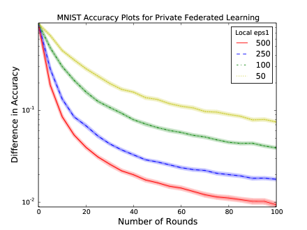
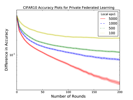
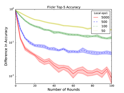
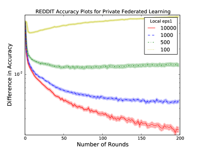
(a)	(b)

Figure 4: Accuracy plots for image classification comparing the private federated learning approach (indexed by privacy parameter $\varepsilon_{1}$) with non-private model updates. Horizontal axis indexes number of stochastic gradient updates, vertical the gap in test-set accuracy between the final non-private model and the private model $\theta_{k}$ at the given round. (a) MNIST dataset. (b) CIFAR-10 dataset.

5.3 Pretrained models

Our final set of experiments investigates refitting a model on a new population. Given the large number of well-established and downloadable deep networks, we view this fine-tuning as a realistic use case for private federated learning.

Image classification on Flickr over 100 classes

We perform our first model tuning experiment on a pre-trained ResNet50v2 network [41] fit using ImageNet data [25], whose reference implementation is available at the website [50]. Beginning from the pre-fit model, we consider only the final (softmax) layer and final convolutional layer of the network to be modifiable, refitting the model to perform 100-class multiclass classification on a subset of the Flickr corpus [65]. There are $d=$ 1,255,524 parameters.

We construct a subsample for each of our experiments as follows. We choose 100 classes (uniformly at random) and $2000$ images from each class, yielding $2\cdot 10^{5}$ images. We randomly permute these into a 9:1 train/test split. In each iteration of the stochastic gradient method, we randomly choose $B=100$ sets of $m=128$ images, performing an approximation to the proximal-point update (11) using 15 gradient steps for each batch $b=1,2,\ldots,B$. Again following the mechanism (23), for the magnitude of each update we use $\texttt{ScalarDP}(\cdot,\varepsilon_{2}=10,k=\lceil e^{\varepsilon_{2}/3}\rceil,r_{\max}=10)$, while for the unit direction we use $\texttt{PrivUnit}_{2}(\cdot,\gamma(0.99\cdot\varepsilon_{1}),p(0.01\cdot\varepsilon_{1}))$ while varying $\varepsilon_{1}$. We present the results in Figure 5(a) for mechanisms that satisfy $(\varepsilon_{1},\varepsilon_{2}=10)$-separated DP where $\varepsilon_{1}\in\{50,100,500,5000\}$. We plot the difference in accuracies between federated learning and our private federated learning system with standard errors over 12 trials.

Next Word Prediction

For our final experiment, we investigate performance of the private federated learning system for next word prediction in a deep word-prediction model. We pretrain an LSTM on a corpus consisting of all Wikipedia entries as of October 1, 2016 [69]. Our model architecture consists of one long-term-short-term memory (LSTM) cell [63] with a word embedding matrix [58] that maps each of 25,003 tokens $j$ (including an unknown, end of sentence, and beginning of sentence tokens) to a vector $w_{j}$ in dimension 256. We use the Natural Language Toolkit (NLTK) tokenization procedure to tokenize each sentence and word [51]. The LSTM cell has 256 units, which leads to 526,336 trainable parameters. Then we decode back into 25,003 tokens. In total, there are $d=$ 13,352,875 trainable parameters in the LSTM.

We refit this pretrained LSTM on a corpus of all user comments on the website Reddit from November 2017 [10], again using the NLTK tokenization procedure [51]. Each stochastic update (13) consists of choosing a random batch of $B=200$ collections of $m=1000$ sentences, performing the local updates (11) approximately by computing 10 gradient steps within each batch $b=1,\ldots,B$. We use update parameters $\texttt{ScalarDP}(\cdot,\varepsilon_{2}=10,k=\lceil e^{\varepsilon_{2}/3}\rceil,r_{\max}=5)$ and $\texttt{PrivUnit}_{2}(\cdot,\gamma(0.99\cdot\varepsilon_{1}),p(0.01\cdot\varepsilon_{1}))$ while varying $\varepsilon_{1}$. We present results in Figure 5(b) for mechanisms that satisfy $(\varepsilon_{1},\varepsilon_{2}=10)$-separated DP where $\varepsilon_{1}\in\{100,500,2500,10000\}$. We choose the centralized projection $\rho=100$ and noise $\sigma$ in the aggregation (13) to guarantee $(\varepsilon_{\textup{cent}}=3,\delta=10^{-9})$ differential privacy after $T=200$ rounds. We plot the difference in accuracies between federated learning and our private federated learning system with standard errors over 20 trials.

(a)	(b)

Figure 5: Accuracy plots for pretrained models comparing our private federated learning approach (labeled SDP with the corresponding $\varepsilon_{1}$ parameter) with various privacy parameter $\varepsilon$ and federated learning with clear model updates (labeled Clear). (a) Top 5 accuracy image classification: top 100 classes from Flickr data with Resnet50v2 model pretrained on ImageNet. (b) Next Word Prediction: Reddit data with pretrained LSTM on Wikipedia data with initial accuracy roughly $15.5\%$.

6 Discussion and conclusion

In this paper, we have described the analysis and implementation—with new, minimax optimal privatization mechanisms—of a system for large-scale distributed model fitting, or federated learning. In such systems, users may prefer local privacy protections, though as this and previous work [31, 26] and make clear, providing small $\varepsilon$-local differential privacy makes model-fitting extremely challenging. Thus, it is of substantial interest to understand what is possible in large $\varepsilon$ regimes, and the corresponding types of privacy such mechanisms provide; we have provided one such justification via prior beliefs and reconstruction probabilities from oblivious adversaries. We believe understanding appropriate privacy barriers, which provide different types of protections at different levels, will be important for the practical adoption of private procedures, and we hope that the current paper provides impetus in this direction.

7 Acknowledgements

We thank Aaron Roth for helpful discussions on earlier versions of this work. His comments helped shape the direction of the paper.

Appendix A Technical proofs

A.1 Proof of Lemma 2.3

We prove each result in turn. We begin with the precision bound. Fix $p>0$, and assume that $pv^{T}\mathbf{1}\geq v^{T}\mathbb{E}[X]$. Then using that ${\rm Var}(v_{j}(X_{j}-\mathbb{E}[X_{j}]))\leq v_{j}\frac{m}{j}$, and is 0 for $j<m$. By Bernstein’s inequality, we then have

$$\mathbb{P}(\mathsf{precision}(v,X)\geq p) =\mathbb{P}(v^{T}(X-\mathbb{E}[X])\geq pv^{T}\mathbf{1}-v^{T}\mathbb{E}[X])$$

$$\leq\exp\left(-\frac{(pv^{T}\mathbf{1}-v^{T}\mathbb{E}[X])^{2}}{2\sum_{j>m}v_{j}{\rm Var}(X_{j})+\frac{2}{3}(pv^{T}\mathbf{1}-v^{T}\mathbb{E}[X])}\right)$$

$$\leq\exp\left(-\min\left\{\frac{(pv^{T}\mathbf{1}-v^{T}\mathbb{E}[X])^{2}}{4\sum_{j>m}v_{j}{\rm Var}(X_{j})},\frac{3}{4}(pv^{T}\mathbf{1}-v^{T}\mathbb{E}[X])\right\}\right)$$ (24)

For $v^{T}\mathbf{1}\geq\gamma m$, assuming that $p\geq\frac{1}{\gamma}$, we have

$$pv^{T}\mathbf{1}-v^{T}\mathbb{E}[X]\geq p\gamma m-\sum_{j=1}^{\gamma m}\mathbb{E}[X_{j}]=p\gamma m-m-\sum_{j=m+1}^{\gamma m}\frac{m}{j}\geq(p\gamma-1)m-m\int_{m}^{\gamma m}\frac{1}{t}dt=(p\gamma-1-\log\gamma)m.$$

For the first term in the exponent (24), the ratio again is maximized by $v=(\mathbf{1}_{\gamma m},\mathbf{0}_{d-\gamma m})$, and we have

$$\sum_{j=m+1}^{d}v_{j}{\rm Var}(X_{j})\leq\sum_{j>m}^{\gamma m}\frac{m}{j}\leq m\int_{m}^{\gamma m}\frac{1}{t}dt=m\log\gamma.$$

Substituting these bounds in Eq. (24), we have

$$\mathbb{P}(\mathsf{precision}(v,X)\geq p)\leq\exp\left(-\min\left\{\frac{(p\gamma-1-\log\gamma)^{2}m}{4\log\gamma},\frac{3}{4}(p\gamma-1-\log\gamma)m\right\}\right).$$

For the recall bounds, we perform a similar derivation, assuming $r\leq\frac{1}{2}$ so that $(1-r)\geq r$. We temporarily assume $(r\mathbf{1}-v)^{T}\mathbb{E}[X]\geq 0$; we shall see that this holds. By Bernstein’s inequality, we have

$$\mathbb{P}(\mathsf{recall}(v,X)\geq r) =\mathbb{P}(v^{T}X\geq r\mathbf{1}^{T}X)=\mathbb{P}((v-r\mathbf{1})^{T}(X-\mathbb{E}[X])\geq(r\mathbf{1}-v)^{T}\mathbb{E}[X])$$

$$\leq\exp\left(-\frac{((r\mathbf{1}-v)^{T}\mathbb{E}[X])^{2}}{2\sum_{j>m}(r-v_{j})^{2}{\rm Var}(X_{j})+\frac{2}{3}(r\mathbf{1}-v)^{T}\mathbb{E}[X]}\right)$$

$$\leq\exp\left(-\min\left\{\frac{((r\mathbf{1}-v)^{T}\mathbb{E}[X])^{2}}{4\sum_{j>m}(r-v_{j})^{2}{\rm Var}(X_{j})},\frac{3}{4}(r\mathbf{1}-v)^{T}\mathbb{E}[X]\right\}\right).$$ (25)

We consider each term in the minimum (25) in turn. When $\sum_{j}v_{j}\leq\gamma m$, we have

$$\sum_{j>m}(r-v_{j}){\rm Var}(X_{j})^{2}\leq m(1-r)^{2}\int_{m}^{d}\frac{1}{t}dt=m(1-r)^{2}\log\frac{d}{m},$$

while

$$(r\mathbf{1}-v)^{T}\mathbb{E}[X] \geq r\mathbf{1}^{T}\mathbb{E}[X]-\sum_{j=1}^{\gamma m}\mathbb{E}[X]=rm+r\sum_{j=m+1}^{d}\frac{m}{j}-m-\sum_{j=m+1}^{\gamma m}\mathbb{E}[X_{j}]$$

$$\geq rm+rm\int_{m+1}^{d}\frac{1}{t}dt-m-m\int_{m}^{\gamma m}\frac{1}{t}dt=m\left[r\left(1+\log\frac{d}{m+1}\right)-1-\log\gamma\right].$$

Substituting into inequality (25) gives the second result of the lemma.

A.2 Proof of Theorem 2

Let $u\in\{-1,+1\}^{d}$ and $U\sim\mathsf{Uni}(\{-1,+1\}^{d})$. The vector $V\in\{-1,1\}^{d}$ sampled as in (18), has p.m.f.

$$p(v\mid u)\propto\begin{cases}1/\mathbb{P}(\langle U,u\rangle>\kappa)&\mbox{if~{}}\langle v,u\rangle>\kappa\\ 1/\mathbb{P}(\langle U,u\rangle<\kappa)&\mbox{if~{}}\langle v,u\rangle\leq\kappa.\end{cases}$$

The event that $\langle U,u\rangle=\kappa$ when $\frac{d+\kappa+1}{2}\in\mathbb{Z}$ implies that $U$ and $u$ match in exactly $\frac{d+\kappa+1}{2}$ coordinates; the number of such matches is $\binom{d}{(d+\kappa+1)/2}$. Computing the binomial sum, we have

$$\mathbb{P}(\langle U,u\rangle>\kappa)=\frac{1}{2^{d}}\sum_{\ell=\lceil\frac{d+\kappa+1}{2}\rceil}^{d}\binom{d}{\ell}\quad\mbox{and}\quad\mathbb{P}(\langle U,u\rangle\leq\kappa)=\frac{1}{2^{d}}\sum_{\ell=0}^{\lceil\frac{d+\kappa+1}{2}\rceil-1}\binom{d}{\ell}.$$

As $\mathbb{P}(\langle U,u\rangle>\kappa)$ is decreasing in $\kappa$ for any $u,u^{\prime}\in\{-1,+1\}^{d}$ and $v\in\{-1,1\}^{d}$ we have

$$\frac{p(v\mid u)}{p(v\mid u^{\prime})}\leq\frac{p_{0}}{1-p_{0}}\cdot\frac{\mathbb{P}(\langle U,u^{\prime}\rangle\leq\kappa)}{\mathbb{P}(\langle U,u\rangle>\kappa)}=e^{\varepsilon_{0}}\cdot\frac{\sum_{\ell=0}^{d\tau-1}\binom{d}{\ell}}{\sum_{\ell=d\tau}^{d}\binom{d}{\ell}},$$

where $\tau=\left\lceil{(d+\kappa)/2}\right\rceil$. Bounding this by $e^{\varepsilon+\varepsilon_{0}}$ gives the result.

A.3 Proof of Corollary 4.1

Using Theorem 2, we seek to bound the quantity (19) for various $\kappa$ values. We first analyze the case when $\kappa\leq\sqrt{3/2d+1}$. We use the following claim to bound each term in the summation in this case.

Claim A.1 (See Problem 1 in [44]).

For even $d\geq 2$, we have

$$\binom{d}{d/2}\leq\frac{2^{d+1/2}}{\sqrt{3d+2}}$$

Thus, when $\kappa<\sqrt{\tfrac{3d+2}{2}}$,

$$\log\left(\sum_{\ell=0}^{d\tau-1}\binom{d}{\ell}\right)-\log\left(\sum_{\ell=d\tau}^{d}\binom{d}{\ell}\right) =\log\left(1/2+\frac{1}{2^{d}}\cdot\sum_{\ell=d/2}^{d\tau-1}\binom{d}{\ell}\right)-\log\left(1/2-\frac{1}{2^{d}}\sum_{\ell=d/2}^{d\tau-1}\binom{d}{\ell}\right)$$

$$\leq\log\left(1+\kappa\cdot\left(\sqrt{\frac{2}{3d+2}}\right)\right)-\log\left(1-\kappa\cdot\left(\sqrt{\frac{2}{3d+2}}\right)\right).$$

Hence, to ensure $\varepsilon$-differential privacy, it suffices to have

$$\varepsilon\geq\log\left(1+\kappa\cdot\sqrt{\frac{2}{3d+2}}\right)-\log\left(1-\kappa\cdot\sqrt{\frac{2}{3d+2}}\right),$$

so Eq. (20) follows.

We now consider the case where $\epsilon=\Omega(\log(d))$. We use the following claim.

Claim A.2 (Lemma 4.7.2 in [4]).

Let $Z\sim\mathsf{Bin}\left(d,1/2\right)$. Then for $0<\lambda<1$, we have

$$\mathbb{P}(Z\geq d\lambda)\geq\frac{1}{\sqrt{8d\lambda(1-\lambda)}}\exp\left(-dD_{\rm kl}\left({\lambda}|\!|{1/2}\right)\right)$$

We then use this to obtain the following bound:

$$\log\left(\sum_{\ell=0}^{d\tau-1}\binom{d}{\ell}\right)-\log\left(\sum_{\ell=d\tau}^{d}\binom{d}{\ell}\right) \leq\frac{1}{2}\log\left(8d\tau(1-\tau)\right)+dD_{\rm kl}\left({\tau}|\!|{1/2}\right)$$

To ensure $\varepsilon$-differential privacy, it is thus sufficient, for $\tau:=\frac{\lceil\frac{d+\kappa+1}{2}\rceil}{d}$, to have

$$\varepsilon \geq\frac{1}{2}\log\left(8\cdot d\tau(1-\tau)\right)+d\cdot D_{\rm kl}\left({\tau}|\!|{1/2}\right),$$

which implies the final claim of the corollary.

A.4 Proof of Lemma 4.5

For shorthand, define the radius $R=\left\|{\nabla\ell(\theta^{\star};X)}\right\|_{2}$, $\gamma=\gamma(\varepsilon_{1})$, let $U=\nabla\ell(\theta^{\star};X)/\left\|{\nabla\ell(\theta^{\star};X)}\right\|_{2}$, and write

$$Z_{1}=\texttt{PrivUnit}_{2}\left(U;\gamma,p=1/2\right)\qquad Z_{2}=\texttt{ScalarDP}(R,\varepsilon_{2};k=\lceil e^{\varepsilon_{2}/3}\rceil,r_{\max})$$

so that $Z=Z_{1}Z_{2}$. Using that $\mathbb{E}[(Z_{2}-R)^{2}\mid R]\leq O(r_{\max}^{2}e^{-2\varepsilon_{2}/3})$ by Lemma 4.4, we have

$$\mathbb{E}[Z(\theta^{\star};X)Z(\theta^{\star};X)^{\top}] =\mathbb{E}\left[\mathbb{E}\left[Z_{1}Z_{1}^{\top}\mid U\right]\cdot\mathbb{E}\left[Z_{2}^{2}\mid R\right]\right]$$

$$=\mathbb{E}\left[\mathbb{E}\left[Z_{1}Z_{1}^{\top}\mid U\right]\cdot\mathbb{E}\left[(Z_{2}-R)^{2}\mid R\right]\right]+\mathbb{E}\left[R^{2}\cdot\mathbb{E}[Z_{1}Z_{1}^{\top}\mid U]\right]$$

$$\preceq O(1)r_{\max}^{2}e^{-2\varepsilon_{2}/3}\cdot\mathbb{E}\left[\mathbb{E}\left[Z_{1}Z_{1}^{\top}\mid U\right]\right]+\mathbb{E}\left[R^{2}\cdot\mathbb{E}[Z_{1}Z_{1}^{\top}\mid U]\right].$$ (26)

We now focus on the term $\mathbb{E}[Z_{1}Z_{1}^{\top}\mid U]$. Recall that $V$ is uniform on $\{v\in\mathbb{S}^{d-1}:\langle v,u\rangle\geq\gamma\}$ with probability $\frac{1}{2}$ and uniform on the complement $\{v\in\mathbb{S}^{d-1}:\langle v,u\rangle<\gamma\}$ otherwise (Eq. (14)). Then for $W\sim\mathsf{Uni}(\mathbb{S}^{d-1})$, we obtain $\mathbb{E}[VV^{\top}\mid u]=\frac{1}{2}\mathbb{E}[WW^{\top}\mid\langle W,u\rangle\geq\gamma]+\frac{1}{2}\mathbb{E}[WW^{\top}\mid\langle W,u\rangle<\gamma]$, where

$$\mathbb{E}[WW^{\top}\mid\langle W,u\rangle\geq\gamma]\preceq uu^{\top}+\frac{1-\gamma^{2}}{d-1}(I_{d}-uu^{\top})~{}~{}~{}\mbox{and}~{}~{}~{}\mathbb{E}[WW^{\top}\mid\langle W,u\rangle\leq\gamma]\preceq uu^{\top}+\frac{1}{d}(I_{d}-uu^{\top}).$$

Both of these are in turn bounded by $uu^{\top}+(1/d)I_{d}$. Using that the normalization $m$ defined in Eq. (15) satisfies $m\gtrsim\min\{\varepsilon_{1},\sqrt{\varepsilon_{1}}\}/\sqrt{d}$ by Proposition 4, we obtain

$$\mathbb{E}[Z_{1}Z_{1}^{\top}\mid U=u] \preceq\frac{1}{m^{2}}uu^{\top}+\frac{1}{dm^{2}}I_{d}\preceq\frac{d}{\varepsilon_{1}\wedge\varepsilon_{1}^{2}}uu^{\top}+\frac{1}{\varepsilon_{1}\wedge\varepsilon_{1}^{2}}I_{d}.$$

Substituting this bound into our earlier inequality (26) and using that $RU=\nabla\ell(\theta^{\star};X)$, we obtain

$$\mathbb{E}[Z(\theta^{\star};X)Z(\theta^{\star};X)^{\top}]\preceq O(1)\cdot\frac{dr^{2}_{\max}e^{-2\varepsilon_{2}/3}}{\varepsilon_{1}\wedge\varepsilon_{1}^{2}}\cdot\mathbb{E}[UU^{\top}+(1/d)I_{d}]$$

$$\qquad~{}+O(1)\cdot\left(\frac{d}{\varepsilon_{1}\wedge\varepsilon_{1}^{2}}\cdot\mathbb{E}\left[\nabla\ell(\theta^{\star};X)\nabla\ell(\theta^{\star};X)^{\top}\right]+\frac{1}{\varepsilon_{1}\wedge\varepsilon_{1}^{2}}\cdot\mathbb{E}\left[\left\|{\nabla\ell(\theta^{\star};X)}\right\|_{2}^{2}I_{d}\right]\right).$$

Noting that $\mathop{\rm tr}(\mathop{\rm Cov}(W))=\mathbb{E}[\left\|{W}\right\|_{2}^{2}]$ for any random vector $W$ gives the lemma.

Appendix B Scalar sampling

B.1 Proof of Lemma 4.3

That the mechanism is $\varepsilon$-differentially private is immediate as randomized response is $\varepsilon$-differentially private. To prove that $Z$ is unbiased, we note that

$$\mathbb{E}[J]=\frac{kr}{r_{\max}}~{}~{}\mbox{and}~{}~{}\mathbb{E}[Z\mid J]=\frac{r_{\max}}{k}J,$$

so that $\mathbb{E}[Z]=\frac{r_{\max}}{r}\mathbb{E}[J]=r$. To develop the bounds on the variance of $Z$, we use the standard decomposition of variance into conditional variances, as

$${\rm Var}(Z)=\mathbb{E}[(Z-r)^{2}]=\mathbb{E}\left[{\rm Var}\left[Z\mid J\right]\right]+{\rm Var}\left[\mathbb{E}\left[Z\mid J\right]\right]=\mathbb{E}[{\rm Var}[Z\mid J]]+\frac{r_{\max}^{2}}{k^{2}}{\rm Var}[J].$$

We have ${\rm Var}[Z\mid J]=a^{2}\cdot{\rm Var}[\widehat{J}\mid J]$. Further, we have

$$\mathbb{E}[\widehat{J}^{2}\mid J]=\left(\frac{e^{\varepsilon}-1}{e^{\varepsilon}+k}\right)\cdot J^{2}+\left(\frac{1}{e^{\varepsilon}+k}\right)\cdot\sum_{j=0}^{k}j^{2}~{}~{}~{}\mbox{and}~{}~{}~{}\mathbb{E}[\widehat{J}\mid J]=\left(\frac{e^{\varepsilon}-1}{e^{\varepsilon}+k}\right)\cdot J+\left(\frac{1}{e^{\varepsilon}+k}\right)\cdot\sum_{j=0}^{k}j.$$

Combining the equalities and using that ${\rm Var}(Y)=\mathbb{E}[Y^{2}]-\mathbb{E}[Y]^{2}$, we have

$${\rm Var}[\widehat{J}\mid J] =\left(\frac{e^{\varepsilon}-1}{e^{\varepsilon}+k}\right)^{2}\cdot\left(\left(\frac{e^{\varepsilon}+k}{e^{\varepsilon}-1}-1\right)\cdot J^{2}-\frac{k(k+1)}{e^{\varepsilon}-1}\cdot J+\frac{k(k+1)(2k+1)(e^{\varepsilon}+k)}{6(e^{\varepsilon}-1)^{2}}-\frac{k^{2}(k+1)^{2}}{4(e^{\varepsilon}-1)^{2}}\right).$$

We then have the conditional variance

$${\rm Var}[Z\mid J] =\frac{r_{\max}^{2}}{(e^{\varepsilon}-1)^{2}}\cdot\left(\frac{(k+1)(e^{\varepsilon}-1)}{k^{2}}\cdot J^{2}-\frac{(k+1)(e^{\varepsilon}-1)}{k}J+\frac{(k+1)(2k+1)(e^{\varepsilon}+k)}{6k}-\frac{(k+1)^{2}}{4}\right).$$

Now, note that $J$ is a Bernoulli sample taking values in $\{\left\lfloor{kr/r_{\max}}\right\rfloor,\left\lceil{kr/r_{\max}}\right\rceil\}$. Thus, recalling the notation $\mathsf{Dec}(t)=\left\lceil{t}\right\rceil-t$ for the decimal part of a number, we have ${\rm Var}(J)=\mathsf{Dec}(\frac{kr}{r_{\max}})(1-\mathsf{Dec}(\frac{kr}{r_{\max}}))$. Substituting all of these above and using that $\mathbb{E}[J^{2}]={\rm Var}(J)+\mathbb{E}[J]^{2}={\rm Var}(J)+\frac{k^{2}r^{2}}{r_{\max}^{2}}$, we obtain

$${\rm Var}(Z)$$

$$=\frac{r_{\max}^{2}}{(e^{\varepsilon}-1)^{2}}\cdot\bigg{(}\frac{(k+1)(e^{\varepsilon}-1)}{k^{2}}\left(\frac{k^{2}r^{2}}{r_{\max}^{2}}+\mathsf{Dec}(kr/r_{\max})(1-\mathsf{Dec}(kr/r_{\max}))\right)~{}\ldots$$

$$\qquad\qquad\qquad~{}-(k+1)(e^{\varepsilon}-1)\frac{r}{r_{\max}}+\frac{(k+1)(2k+1)(e^{\varepsilon}+k)}{6k}-\frac{(k+1)^{2}}{4}\bigg{)}$$

$$\qquad~{}+\frac{r_{\max}^{2}}{k^{2}}\mathsf{Dec}(kr/r_{\max})(1-\mathsf{Dec}(kr/r_{\max}))$$

$$\leq\frac{k+1}{e^{\varepsilon}-1}\left[r^{2}+\frac{r_{\max}^{2}}{4k^{2}}-rr_{\max}+\frac{(2k+1)(e^{\varepsilon}+k)r_{\max}^{2}}{6k(e^{\varepsilon}-1)}-\frac{k+1}{4(e^{\varepsilon}-1)}\right]+\frac{r_{\max}^{2}}{4k^{2}}$$

where we have used that $p(1-p)\leq\frac{1}{4}$ for all $p\in[0,1]$. Ignoring the negative terms gives the result.

B.2 Sampling scalars with relative error

As our discussion in the introductory Section 1.2 shows, to develop optimal learning procedures it is frequently important to know when the problem is easy—observations are low variance—and for this, releasing scalars with relative error can be important. Consequently, we consider an alternative mechanism that first breaks the range $[0,r_{\max}]$ into intervals of increasing length based on a fixed accuracy $\alpha>0$, $k\in\mathbb{N}$, and $\nu>1$, where we define the intervals

$$E_{0}=[0,\nu\alpha],~{}~{}E_{i}=[\nu^{i}\alpha,\nu^{i+1}\alpha]~{}\mbox{for~{}}i=1,\ldots,{k-1}.$$ (27)

The resulting mechanism works as follows: we determine the interval that $r$ belongs to, we randomly round $r$ to an endpoint of the interval (in an unbiased way), then use randomized response to obtain a differentially private quantity, which we then debias. We formalize the algorithm in Algorithm 4.

Algorithm 4 Privatize the magnitude with relative error: ScalarRelDP

Magnitude $r$, privacy parameter $\varepsilon>0$, integer $k$, accuracy $\alpha>0$, $\nu>1$, bound $r_{\max}$.

$r\leftarrow\min\{r,r_{\max}\}$

Form the intervals $\{E_{0},E_{1},\cdots,E_{k-1}\}$ given in (27) and let $i^{*}$ be the index such that $r\in E_{i^{*}}$.

Sample $J\in\{0,1,\cdots,k\}$ such that

$$J=\begin{cases}0&\mbox{w.p.}~{}\frac{\nu\alpha-r}{\nu\alpha}\\ 1&\mbox{w.p.}~{}\frac{r}{\nu\alpha}\end{cases}~{}~{}\mbox{if~{}}i^{*}=0\,~{}~{}~{}\mbox{and}~{}~{}~{}J=\begin{cases}i^{*}&\mbox{w.p.}~{}\frac{\nu^{i^{*}+1}\alpha-r}{\nu^{i^{*}}(\nu-1)\alpha}\\ i^{*}+1&\mbox{w.p.}~{}\frac{r-\nu^{i^{*}}\alpha}{\nu^{i^{*}}(\nu-1)\alpha}\end{cases}~{}~{}\mbox{if~{}}i^{*}\geq 1.$$

Use randomized response to obtain $\widehat{J}$

$$\widehat{J}\mid(J=i)=\begin{cases}i&\mbox{w.p.}~{}\frac{e^{\varepsilon}}{e^{\varepsilon}+k}\\ \mbox{uniform in~{}}\{0,\ldots,k\}\setminus i&\mbox{w.p.}~{}\frac{k}{e^{\varepsilon}+k}.\end{cases}$$

Set $\tilde{J}=\nu^{\hat{J}}\cdot\mathbbm{1}\left\{\hat{J}\geq 1\right\}$

Debias $\tilde{J}$, by setting

$$Z=a\left(\tilde{J}-b\right)~{}~{}\mbox{for~{}}a=\alpha\cdot\left(\frac{e^{\varepsilon}+k}{e^{\varepsilon}-1}\right)~{}~{}\mbox{and}~{}~{}b=\frac{1}{e^{\varepsilon}+k}\cdot\sum_{j=1}^{k}\nu^{j}.$$

return $Z$

As in the absolute erorr case, we can provide an upper bound on the error of the mechanism ScalarRelDP, though in this case—up to the small accuracy $\alpha$—our error guarantee is relative.

Lemma B.1.

Fix $\alpha>0$, $k\in\mathbb{N}$, and $\nu>1$. Then $Z=\texttt{ScalarRelDP}(\cdot,\varepsilon;k,\alpha,\nu,r_{\max})$ is $\varepsilon$-differentially private and for $r<r_{\max}$, we have $\mathbb{E}[Z\mid r]=r$ and

$$\frac{\mathbb{E}[(Z-r)^{2}\mid r]}{(r\vee\alpha)^{2}} \leq\frac{(k+1)}{(e^{\varepsilon}-1)}\nu^{2}+\left(\frac{\nu^{2k}\cdot(e^{\varepsilon}+k)}{(e^{\varepsilon}-1)^{2}}\right)\left(\frac{1-\nu^{-2k}}{1-\nu^{-2}}\right)+(\nu-1)^{2}.$$

See Appendix B.3 for a proof of Lemma B.1.

We perform a few calculations with Lemma B.1 when $k\leq e^{\varepsilon}$. Let $\nu=1+\Delta$ for a $\Delta\in(0,1)$ to be chosen, and note that the choice

$$k=\left\lceil{\frac{\log\frac{r_{\max}}{\alpha}}{\log\nu}}\right\rceil\approx\frac{\log\frac{r_{\max}}{\alpha}}{\Delta}$$

is the smallest value of $k$ that gives $\nu^{k}\alpha\geq r_{\max}$. Let $\alpha=r_{\max}\alpha_{0}$, so that $\nu^{2k}\approx\frac{1}{\alpha_{0}^{2}}$. Hence, from Lemma B.1 we have the truncated relative error bound

$$\frac{\mathbb{E}[(Z-r)^{2}\mid r]}{(r\vee r_{\max}\alpha_{0})^{2}}\lesssim\frac{k}{e^{\varepsilon}}+\frac{e^{-\varepsilon}}{\alpha_{0}^{2}\cdot\Delta}+\Delta^{2}=e^{-\varepsilon}\left(\log\frac{1}{\alpha_{0}}+\frac{1}{\alpha_{0}^{2}}\right)\cdot\left(\frac{1}{\Delta}\right)+\Delta^{2}\lesssim\frac{1}{e^{\varepsilon}\alpha_{0}^{2}\Delta}+\Delta^{2}.$$

We assume the relative accuracy threshold $\alpha/r_{\max}=\alpha_{0}\gtrsim e^{-\varepsilon/2}$. Then setting $\Delta=\alpha_{0}^{-2/3}e^{-\varepsilon/3}$ gives

$$\frac{\mathbb{E}[(Z-r)^{2}\mid r]}{(r\vee r_{\max}\alpha_{0})^{2}}\lesssim\alpha_{0}^{-4/3}e^{-2\varepsilon/3}.$$ (28)

Let us compare with Lemma 4.4, which yields

$$\mathbb{E}[(Z-r)^{2}\mid r]=O\left(r_{\max}^{2}e^{-2\varepsilon/3}\right).$$

The choice $\alpha_{0}=1$ in inequality (28) shows that the geometrically-binned mechanism can recover this bound. For $r\leq r_{\max}\alpha_{0}$, the former inequality (28) is stronger; for example, the choice $\alpha_{0}=e^{-\varepsilon/4}$ yields that $\mathbb{E}[(Z-r)^{2}\mid r]=O(r_{\max}^{2}e^{-5\varepsilon/6})$ for $r\leq r_{\max}e^{-\varepsilon/4}$, and $\mathbb{E}[(Z-r)^{2}\mid r]=O(r^{2}e^{-\varepsilon/3})$ otherwise.

B.3 Proof of Lemma B.1

To see that $\texttt{ScalarRelDP}(\cdot,k,\alpha,\nu;\varepsilon,r_{\max})$ is differentially private, we point out that randomized response is $\varepsilon$-DP and then DP is closed under post-processing. To see that $Z$ is unbiased, note that

$$\mathbb{E}[\tilde{J}\mid J=i]=\left(\frac{e^{\varepsilon}-1}{e^{\varepsilon}+k}\right)\nu^{i}\mathbbm{1}\left\{i\geq 1\right\}+\frac{1}{e^{\varepsilon}+k}\sum_{j=1}^{k}\nu^{j},$$

and thus for $r\in E_{i^{*}}$,

$$\mathbb{E}[Z] =a\cdot(\mathbb{E}[\hat{J}]-b)=\alpha\cdot\left(\frac{e^{\varepsilon}+k}{e^{\varepsilon}-1}\right)\left(\left(\frac{e^{\varepsilon}-1}{e^{\varepsilon}+k}\right)\mathbb{E}[\nu^{J}\mathbbm{1}\left\{J\geq 1\right\}]+\frac{1}{e^{\varepsilon}+k}\cdot\sum_{j=1}^{k}\nu^{j}-\frac{1}{e^{\varepsilon}+k}\cdot\sum_{j=1}^{k}\nu^{j}\right)$$

$$=\alpha\cdot\mathbb{E}\left[\nu^{J}\mathbbm{1}\left\{J\geq 1\right\}\right]$$

$$=\alpha\cdot\left[\mathbbm{1}\left\{i^{*}=0\right\}\cdot\left(\frac{r}{\alpha\nu}\right)\cdot\nu+\mathbbm{1}\left\{i^{*}\geq 1\right\}\cdot\left(\left(\frac{\nu^{i^{*}+1}\alpha-r}{\nu^{i^{*}}(\nu-1)\alpha}\right)\cdot\nu^{i^{*}}+\left(\frac{r-\nu^{i^{*}}\alpha}{\nu^{i^{*}}(\nu-1)\alpha}\right)\cdot\nu^{i^{*}+1}\right)\right]$$

$$=\mathbbm{1}\left\{i^{*}=0\right\}\cdot r+\mathbbm{1}\left\{i^{*}\geq 1\right\}\cdot r=r$$

Consider the following mean squared error terms

$$\mathbb{E}\left[(r-\alpha\nu^{J}\cdot\mathbbm{1}\left\{J\geq 1\right\})^{2}\mid r\in E_{0}\right] =r^{2}\left(1-\frac{r}{\alpha\nu}\right)+(r-\alpha\nu)^{2}\left(\frac{r}{\alpha\nu}\right)=r\left(\alpha\nu-r\right)\leq(\nu\alpha)^{2}$$

And for $i^{*}\geq 1$

$$\mathbb{E}\left[(r-\alpha\nu^{J}\cdot\mathbbm{1}\left\{J\geq 1\right\})^{2}\mid r\in E_{i^{*}}\right]\leq(\nu^{i^{*}+1}\alpha-\nu^{i^{*}}\alpha)^{2}=\nu^{2i^{*}}(\nu^{i^{*}}-1)^{2}\alpha^{2}.$$

We then bound the conditional expectation

$${\rm Var}(Z\mid J=i^{*})=a^{2}{\rm Var}(\tilde{J}\mid J=i^{*})=\alpha^{2}\cdot\left(\frac{e^{\varepsilon}+k}{e^{\varepsilon}-1}\right)\cdot{\rm Var}(\tilde{J}\mid J=i^{*}),$$

Now we note that

$${\rm Var}(\tilde{J}\mid J=i^{*}) =\left(\frac{e^{\varepsilon}-1}{e^{\varepsilon}+k}\right)\cdot\nu^{2i^{*}}\mathbbm{1}\left\{i^{*}\geq 1\right\}+\left(\frac{1}{e^{\varepsilon}+k}\right)\cdot\sum_{j=1}^{k}\nu^{2j}$$

$$\qquad-\left(\left(\frac{e^{\varepsilon}-1}{e^{\varepsilon}+k}\right)\cdot\nu^{i^{*}}\mathbbm{1}\left\{i^{*}\geq 1\right\}+\left(\frac{1}{e^{\varepsilon}+k}\right)\cdot\sum_{j=1}^{k}\nu^{j}\right)^{2}$$

$$\leq\left(\frac{(k+1)(e^{\varepsilon}-1)}{(e^{\varepsilon}+k)^{2}}\right)\cdot\nu^{2i^{*}}\mathbbm{1}\left\{i^{*}\geq 1\right\}+\left(\frac{1}{e^{\varepsilon}+k}\right)\cdot\nu^{2k}\cdot\sum_{j=0}^{k-1}\nu^{-2j}$$

$$=\left(\frac{(k+1)(e^{\varepsilon}-1)}{(e^{\varepsilon}+k)^{2}}\right)\cdot\nu^{2i^{*}}\mathbbm{1}\left\{i^{*}\geq 1\right\}+\left(\frac{1}{e^{\varepsilon}+k}\right)\cdot\nu^{2k}\cdot\left(\frac{1-\nu^{-2k}}{1-\nu^{-2}}\right).$$

Now, if $r\in E_{i^{*}}$, we have that $\nu^{i^{*}}\alpha\leq(r\vee\alpha)\leq\nu^{i^{*}+1}\alpha$, and thus

$$\frac{\mathbb{E}[(Z-r)^{2}]}{(r\vee\alpha)^{2}} \leq\frac{\alpha^{2}}{(r\vee\alpha)^{2}}\cdot\left(\frac{e^{\varepsilon}+k}{e^{\varepsilon}-1}\right)^{2}\cdot\left[\frac{(k+1)(e^{\varepsilon}-1)}{(e^{\varepsilon}+k)^{2}}\nu^{2(i^{*}+1)}+\frac{\nu^{2k}}{e^{\varepsilon}+k}\left(\cdot\frac{1-\nu^{-2k}}{1-\nu^{-2}}\right)\right]$$

$$\qquad+\frac{\alpha^{2}}{(r\vee\alpha)^{2}}\cdot\nu^{2i^{*}}(\nu-1)^{2}$$

$$\leq\frac{(k+1)}{(e^{\varepsilon}-1)}\nu^{2}+\left(\frac{\nu^{2k}\cdot(e^{\varepsilon}+k)}{(e^{\varepsilon}-1)^{2}}\right)\left(\frac{1-\nu^{-2k}}{1-\nu^{-2}}\right)+(\nu-1)^{2},$$

as desired.

Appendix C Proofs of utility in private sampling mechanisms

C.1 Proof of Lemma 4.1

Let $u\in\mathbb{S}^{d-1}$ and $U\in\mathbb{S}^{d-1}$ be a uniform random variable on the unit sphere. Then rotational symmetry implies that for some $\gamma_{+}>0>\gamma_{-}$,

$$\mathbb{E}[U\mid\langle U,u\rangle\geq\gamma]=\gamma_{+}\cdot u~{}~{}\mbox{and}~{}~{}\mathbb{E}[U\mid\langle U,u\rangle<\gamma]=\gamma_{-}\cdot u,$$

and similarly, the random vector $V$ in Algorithm 1 satisfies

$$\mathbb{E}[V\mid u]=p\mathbb{E}[U\mid\langle U,u\rangle\geq\gamma]+(1-p)\cdot\mathbb{E}[U\mid\langle U,u\rangle<\gamma]=p(\gamma_{+}+\gamma_{-})\cdot u.$$

By rotational symetry, we may assume $u=e_{1}$, the first standard basis vector, without loss of generality. We now compute the normalization constant. Letting $U\sim\mathsf{Uni}(\mathbb{S}^{d-1})$ have coordinates $U_{1},\ldots,U_{d}$, we marginally $U_{i}\stackrel{{\scriptstyle\rm dist}}{{=}}2B-1$ where $B\sim\mathsf{Beta}(\frac{d-1}{2},\frac{d-1}{2})$. Now, we note that

$$\gamma_{+}=\mathbb{E}[U_{1}\mid U_{1}\geq\gamma]=\mathbb{E}[2B-1\mid B\geq\tfrac{1+\gamma}{2}]~{}~{}~{}\mbox{and}~{}~{}~{}\gamma_{-}=\mathbb{E}[U_{1}\mid U_{1}<\gamma]=\mathbb{E}[2B-1\mid B<\tfrac{1+\gamma}{2}]$$

and that if $B\sim\mathsf{Beta}(\alpha,\beta)$, then for $0\leq\tau\leq 1$, we have

$$\mathbb{E}[B\mid B\geq\tau] =\frac{1}{B(\alpha,\beta)\cdot\mathbb{P}(B\geq\tau)}\int_{\tau}^{1}x^{\alpha}(1-x)^{\beta-1}dx=\frac{B(\alpha+1,\beta)-B(\tau;\alpha+1,\beta)}{B(\alpha,\beta)-B(\tau;\alpha,\beta)}$$

and similarly $\mathbb{E}[B\mid B<\tau]=\frac{B(\tau;\alpha+1,\beta)}{B(\tau;\alpha,\beta)}$. Using that $B(\tau;\alpha+1,\alpha)=B(\alpha+1,\alpha)[\frac{B(\tau;\alpha,\alpha)}{B(\alpha,\alpha)}-\frac{\tau^{\alpha}(1-\tau)^{\alpha}}{\alpha B(\alpha,\alpha)}]$ and $B(\alpha+1,\alpha)=\frac{1}{2}B(\alpha,\alpha)$, then substituting in our calculation for $\gamma_{+}$ and $\gamma_{-}$, we have for $\tau=\frac{1+\gamma}{2}$ and $\alpha=\frac{d-1}{2}$ that

$$\gamma_{+}=\frac{1}{\alpha\cdot 2^{d-1}}\cdot\frac{(1-\gamma^{2})^{\alpha}}{B(\alpha,\alpha)-B(\tau;\alpha,\alpha)}~{}~{}~{}\mbox{and}~{}~{}~{}\gamma_{-}=\frac{-1}{\alpha 2^{d-1}}\cdot\frac{(1-\gamma^{2})^{\alpha}}{B(\tau;\alpha,\alpha)}$$

Consequently, $\mathbb{E}[V\mid u]=(p\gamma_{+}+(1-p)\gamma_{-})u$, and if $Z=\texttt{PrivUnit}_{2}(u,\gamma,p)$ we have $\mathbb{E}[Z]=u$ as desired.

C.2 Proof of Proposition 4

Recall from the proof of Lemma 4.1 that $Z=\frac{1}{p\gamma_{+}+(1-p)\gamma_{-}}V$, where $\mathbb{E}[U\mid\langle U,u\rangle\geq\gamma]=\gamma_{+}\cdot u$ and $\mathbb{E}[U\mid\langle U,u\rangle<\gamma]=\gamma_{-}\cdot u$ for $U=(U_{1},\cdots,U_{d})\sim\mathsf{Uni}(\mathbb{S}^{d-1})$, so that $\gamma_{+}=\mathbb{E}[U_{1}\mid U_{1}\geq\gamma]\geq\gamma$ and, using $\mathbb{E}[|U_{1}|]\leq\mathbb{E}[U_{1}^{2}]^{1/2}\leq 1/\sqrt{d}$, we have $\gamma_{-}=\mathbb{E}[U_{1}\mid U_{1}\leq\gamma]\in[-\mathbb{E}[|U_{1}|],0]\in[-1/\sqrt{d},0]$. Summarizing, we always have

$$\gamma\leq\gamma_{+}\leq 1,~{}~{}~{}-\frac{1}{\sqrt{d}}\leq\gamma_{-}\leq 0,~{}~{}~{}\mbox{and}~{}~{}~{}|\gamma_{+}|>|\gamma_{-}|.$$

As a consequence, as the norm of $V$ is 1 and $\left\|{Z}\right\|_{2}=1/(p\gamma_{+}+(1-p)\gamma_{-})$, which is decreasing to $1/\gamma_{+}$ as $p\uparrow 1$, we always have $\left\|{Z}\right\|_{2}\leq\frac{2}{\gamma_{+}+\gamma_{-}}$ and we may assume w.l.o.g. that $p=\frac{1}{2}$ in the remainder of the derivation.

Now, we consider three cases in the inequalities (16), deriving lower bounds on $\gamma_{+}+\gamma_{-}$ for each.

1. First, assume $5\leq\varepsilon\leq 2\log d$. Let $\gamma=\gamma_{0}\sqrt{2/d}$ for some $\gamma_{0}\geq 1$. Then the choice $\gamma_{0}=1$ guarantees that second inequality of (16b) holds, while we note that we must have $\gamma_{0}^{2}\leq\frac{d}{d-1}\varepsilon$, as otherwise $\frac{d-1}{2}\log(1-\gamma_{0}^{2}\frac{2}{d})\leq-\frac{d-1}{d}\gamma_{0}^{2}<-\varepsilon$, contradicting the inequality (16b). For $\gamma_{0}\in[1,\sqrt{\frac{d}{d-1}\varepsilon}]$, we have $\log(1-\gamma_{0}^{2}\frac{2}{d})\geq-\frac{8\gamma_{0}^{2}}{3d}$ for sufficiently large $d$, and solving the first inequality in Eq. (16b) we see it is sufficient that

   $$\frac{4(d-1)}{3d}\gamma_{0}^{2}\leq\varepsilon-\log\frac{2d\varepsilon}{d-1}-\log 6~{}~{}\mbox{or}~{}~{}\gamma^{2}\leq\frac{6\varepsilon-6\log 6-3\log\frac{2d\varepsilon}{d-1}}{4(d-1)}.$$

   With this choice of $\gamma$, we obtain $\gamma_{+}+\gamma_{-}\geq c\sqrt{\frac{d}{\varepsilon}}$ for a numerical constant $c$.

2. For $d\geq\varepsilon\geq 5$, it is evident that (for some numerical constant $c$) the choice $\gamma=c\sqrt{\varepsilon/d}$ satisfies inequality (16b). Thus $\gamma_{+}+\gamma_{-}\geq c\sqrt{\frac{d}{\varepsilon}}$.

3. Finally, we consider the last case that $\varepsilon\leq 5$. In this case, the choice $\gamma^{2}=\pi(e^{\varepsilon}-1)^{2}/(2d(e^{\varepsilon}+1)^{2})$ satisfies inequality (16a). We need to control the difference $\gamma_{+}+\gamma_{-}=\mathbb{E}[U_{1}\mid U_{1}\geq\gamma]+\mathbb{E}[U_{1}\mid U_{1}\leq\gamma]$. In this case, let $p_{+}=\mathbb{P}(\langle U,u\rangle\geq\gamma)$ and $p_{-}=\mathbb{P}(\langle U,u\rangle<\gamma)$, so that Lemma D.3 implies that $p_{+}\leq\frac{1}{2}-e^{-2}\gamma\sqrt{\frac{d-1}{2\pi}}$ and $p_{-}\geq\frac{1}{2}+\gamma\sqrt{\frac{d-1}{2\pi}}$. Then

   $$\mathbb{E}[U_{1}\mid U_{1}\geq\gamma]+\mathbb{E}[U_{1}\mid U_{1}<\gamma] =\frac{1}{p_{+}}\mathbb{E}[U_{1}\cdot\mathbbm{1}\left\{U_{1}\geq\gamma\right\}]+\frac{1}{p_{-}}\mathbb{E}[U_{1}\cdot\mathbbm{1}\left\{U_{1}<\gamma\right\}]$$

   $$=\left(\frac{1}{p_{+}}-\frac{1}{p_{-}}\right)\mathbb{E}[U_{1}\cdot\mathbbm{1}\left\{U_{1}\geq\gamma\right\}]\geq\left(1-\frac{p_{+}}{p_{-}}\right)\mathbb{E}[U_{1}\mid U_{1}\geq 0],$$

   where the second equality follows from the fact that $\mathbb{E}[U_{1}]=0$. Using that $\mathbb{E}[U_{1}\mid U_{1}\geq 0]\geq cd^{-1/2}$ for a numerical constant $c$ and

   $$1-\frac{p_{+}}{p_{-}}\geq\frac{4e^{-2}\sqrt{\tfrac{2(d-1)}{\pi}}}{1+2e^{-2}\gamma\sqrt{\tfrac{2(d-1)}{\pi}}}=\Omega\left(\frac{e^{\varepsilon}-1}{e^{\varepsilon}+1}\right)$$

   by our choice of $\gamma$, we obtain $\gamma_{+}+\gamma_{-}\gtrsim(e^{\varepsilon}-1)\sqrt{d}$.

Combining the three cases above, we use that $V$ in Alg. 1 has norm $\left\|{V}\right\|_{2}=1$ and

$$\left\|{Z}\right\|_{2}\leq\frac{2}{\gamma_{+}+\gamma_{-}}\left\|{V}\right\|_{2}\leq c\sqrt{d\cdot\max\left\{\varepsilon^{-1},\varepsilon^{-2}\right\}}$$

to obtain the first result of the proposition.

The final result of the proposition is immediate by the bound on $\left\|{Z}\right\|_{2}$.

C.3 Proof of Lemma 4.2

Without loss of generality, assume that $u\in\{-1,1\}^{d}$, as it is clear that $\mathbb{E}[\widehat{U}\mid u]=u$ in Algorithm 2. We now show that given $u$, $\mathbb{E}[V\mid u=u]=m\cdot u$. Consider $U\sim\mathsf{Uni}(\{-1,+1\}^{d})$, in which case

$$\mathbb{E}[V\mid u=u]=p\mathbb{E}[U\mid\langle U,u\rangle>\kappa]+(1-p)\mathbb{E}[U\mid\langle U,u\rangle\leq\kappa].$$

For constants $\kappa_{+},\kappa_{-}$, uniformity of $U$ implies that

$$\mathbb{E}[U\mid\langle U,u\rangle>\kappa]=\kappa_{+}\cdot u\qquad\mbox{and}\qquad\mathbb{E}[U\mid\langle U,u\rangle\leq\kappa]=\kappa_{-}\cdot u.$$

By symmetry it is no loss of generality to assume that $u=(1,1,\cdots,1)$, so $\langle U,u\rangle=\sum_{\ell=1}^{d}U_{\ell}$. We then have for $\tau=\lceil\frac{d+\kappa+1}{2}\rceil/d$ that

$$\mathbb{E}[U_{1}\mid\langle U,u\rangle>\kappa]=\frac{1}{2^{d}\cdot\mathbb{P}(\langle U,u\rangle>\kappa)}\cdot\sum_{\ell=d\tau}^{d}\left(\binom{d-1}{\ell-1}-\binom{d-1}{\ell}\right)=\frac{\binom{d-1}{d\tau-1}}{\sum_{\ell=d\tau}^{d}\binom{d}{\ell}}=:\kappa_{+}$$

and

$$\mathbb{E}[U_{1}\mid\langle U,u\rangle\leq\kappa]=\frac{1}{2^{d}\cdot\mathbb{P}(\langle U,u\rangle\leq\kappa)}\cdot\sum_{\ell=0}^{d\tau-1}\left(\binom{d-1}{\ell-1}-\binom{d-1}{\ell}\right)=\frac{-\binom{d-1}{d\tau-1}}{\sum_{\ell=0}^{d\tau-1}\binom{d}{\ell}}=:\kappa_{-}.$$

Putting these together and setting $m=p\kappa_{+}+(1-p)\kappa_{-}$, we have $\mathbb{E}[(1/m)V\mid u]=u$.

C.4 Proof of Proposition 5

Using the notation of the proof of Lemma 4.2, the debiasing multiplier $m$ satisfies $1/m=\frac{1}{p\kappa_{+}+(1-p)\kappa_{-}}\leq\frac{2}{\kappa_{+}+\kappa_{-}}$, as $p\geq\frac{1}{2}$. Thus, we seek to lower bound $\kappa_{+}+\kappa_{-}$ by lower bounding $\kappa_{+}$ and $\kappa_{-}$ individually. We consider two cases: the case that $\varepsilon\geq\log d$ and the case that $\varepsilon<\log d$.

Case 1:

when $\varepsilon\geq\log d$. We first focus on lower bounding

$$\kappa_{+}=\frac{\binom{d-1}{d\tau-1}}{\sum_{\ell=d\tau}^{d}\binom{d}{\ell}}=\tau\cdot\frac{\binom{d}{d\tau}}{\sum_{\ell=d\tau}^{d}\binom{d}{\ell}}=\tau\cdot\left(\sum_{\ell=d\tau}^{d}\binom{d}{d\tau}^{-1}\binom{d}{\ell}\right)^{-1}.$$

We argue that eventually the terms in the summation become small. For $\ell\geq d\tau$ defining

$$r:=\frac{d\tau+1}{d-d\tau}\leq\frac{\ell+1}{d-\ell}=\frac{\binom{d}{\ell}}{\binom{d}{\ell+1}}~{}~{}~{}\mbox{implies}~{}~{}~{}\binom{d}{\ell}\geq r\binom{d}{\ell+1},$$

We then have

$$\sum_{\ell=d\tau}^{d}\binom{d}{d\tau}^{-1}\binom{d}{\ell}=\sum_{i=0}^{d-d\tau}\binom{d}{d\tau}^{-1}\binom{d}{d\tau+i}\leq\sum_{i=0}^{d-d\tau}\binom{d}{d\tau}^{-1}\binom{d}{d\tau}\left(\frac{1}{r}\right)^{i}=\sum_{i=0}^{d-d\tau}\frac{1}{r^{i}}\leq\frac{1}{1-1/r},$$

so that

$$\kappa_{+}\geq 1-1/r=1-\frac{d-d\tau}{d\tau+1}=\frac{2d\tau-d+1}{d\tau+1}=\begin{cases}2\cdot\frac{\kappa+2}{d+\kappa+3}&\text{for odd }d+\kappa\\ 2\cdot\frac{\kappa+3}{d+\kappa+4}&\text{for even }d+\kappa\end{cases}\geq\frac{\kappa}{d}.$$ (29)

We now lower bound $\kappa_{-}$, where we use the fact that $d\tau-1\geq\frac{d-1}{2}$ for $\kappa\in\{0,1,\cdots,d\}$ to obtain

$$\kappa_{-}=\frac{-\binom{d-1}{d\tau-1}}{\sum_{\ell=0}^{\tau\cdot d-1}\binom{d}{\ell}}=-\tau\frac{\binom{d}{d\tau}}{\sum_{\ell=0}^{d\tau-1}\binom{d}{\ell}}\geq-\tau\frac{\binom{d}{d\tau}}{2^{d-1}}.$$

Using Stirling’s approximation and that $\tau=\lceil\frac{d+\kappa+1}{2}\rceil/d$, we have

$$\binom{d}{d\tau}=C(\kappa,d)\sqrt{\frac{1}{d}}\cdot 2^{d}\cdot\exp\left(-\frac{\kappa^{2}}{2d}\right),$$

where $C(\kappa,d)$ is upper and lower bounded by positive universal constants. Hence, we have for a constant $c<\infty$,

$$\kappa_{-}\geq-c\cdot\left(\frac{1}{\sqrt{d}}\cdot\exp\left(\frac{-\kappa^{2}}{2d}\right)\right).$$ (30)

An inspection of the bound (21) shows that the choice $\kappa=c\sqrt{\varepsilon d}$ for some (sufficiently small) constant $c$ immediately satisfies the sufficient condition for Algorithm 2 to be private. Substituting this choice of $\kappa$ into the lower bounds (29) and (30) gives that the normalizer $m^{-1}\leq\frac{2}{\kappa_{+}+\kappa_{-}}\lesssim\sqrt{d/\varepsilon}$, which is first result of Proposition 5.

Case 2:

when $\varepsilon<\log d$. In this case, we use the bound (20) to obtain the result. Let us first choose $\kappa$ to saturate the bound (20), for which it suffices to choose $\kappa=c\min\{\sqrt{d},\varepsilon\sqrt{d}\}$ for a numerical constant $c>0$. We assume for simplicity that $d$ is even, as extending the argument is simply notational. Defining the shorthand $s_{\tau}:=\frac{1}{2^{d-1}}\sum_{\ell=d/2}^{d\tau-1}\binom{d}{\ell}$, we recall the definitions of $\kappa_{+}$ and $\kappa_{-}$ to find

$$\kappa_{+}=\tau\cdot\binom{d}{d\tau}\cdot\frac{1}{1-s_{\tau}}~{}~{}~{}\mbox{and}~{}~{}~{}\kappa_{-}=\tau\cdot\binom{d}{d\tau}\cdot\frac{1}{1+s_{\tau}}.$$

Using the definition of the debiasing normalizer $m=p\kappa_{+}+(1-p)\kappa_{-}\geq\frac{1}{2}(\kappa_{+}+\kappa_{-})$, we obtain

$$m \geq\frac{\tau}{2^{d}}\binom{d}{d\tau}\left(\frac{1}{1-s_{\tau}}-\frac{1}{1+s_{\tau}}\right)=\frac{\tau}{2^{d}}\binom{d}{d\tau}\frac{2s_{\tau}}{1-s_{\tau}^{2}}.$$

By definition of $s_{\tau}$, we have $s_{\tau}\geq\frac{d\tau-d/2}{2^{d-1}}\binom{d}{d\tau}\geq\frac{\kappa}{2^{d}}\binom{d}{d\tau}$, so that

$$m \gtrsim\tau\kappa\left(2^{-d}\binom{d}{d\tau}\right)^{2}\gtrsim\frac{1}{d}\kappa\exp\left(-\frac{\kappa^{2}}{d}\right),$$

where the second inequality uses Stirling’s approximation. Our choice of $\kappa=c\min\{\sqrt{d},\varepsilon\sqrt{d}\}$ thus yields $m\gtrsim\frac{1}{\sqrt{d}}\min\{1,\varepsilon\}$, which gives the second result of Proposition 5.

Appendix D Uniform random variables and concentration

In this section, we collect a number of results on the concentration properties of variables uniform on the unit sphere $\mathbb{S}^{d-1}$, which allow our analysis of the mechanism $\texttt{PrivUnit}_{2}$ for privatizing vectors in the $\ell_{2}$ ball in Algorithm 1. For a vector $u\in\mathbb{S}^{d-1}$, that is, satisfying $\left\|{u}\right\|_{2}=1$, and $a\in[0,1]$ we define the spherical cap

$$C(a,u):=\left\{v\in\mathbb{S}^{d-1}\mid\langle v,u\rangle>a\right\}.$$

There are a number of bounds on the probability that $U\in C(a,u)$ for a fixed $u\in\mathbb{S}^{d-1}$ where $U\sim\mathsf{Uni}(\mathbb{S}^{d-1})$, which the following lemma summarizes.

Lemma D.1.

Let $U$ be uniform on the unit sphere $\mathbb{S}^{d-1}$ in $\mathbb{R}^{d}$. Then for $\sqrt{2/d}\leq a\leq 1$ and $u\in\mathbb{S}^{d-1}$,

$$\frac{1}{6a\sqrt{d}}(1-a^{2})^{\frac{d-1}{2}}\leq\mathbb{P}(U\in C(a,u))\leq\frac{1}{2a\sqrt{d}}(1-a^{2})^{\frac{d-1}{2}}.$$ (31)

For all $0\leq a\leq 1$, we have

$$\frac{(1-a)}{2d}(1-a^{2})^{\frac{d-1}{2}}\leq\mathbb{P}(U\in C(a,u))$$ (32)

and for $a\in[0,1/\sqrt{2}]$,

$$\mathbb{P}(U\in C(a,u))\leq(1-a^{2})^{\frac{d}{2}}.$$

Proof    The first result is [16, Exercise 7.9]. The lower bound of the second is due to [57, Lemma 4.1], while the third inequality follows for all $a\in[0,1/\sqrt{2}]$ by [8, Proof of Lemma 2.2]. ∎

We also require a slightly different lemma for small values of the threshold $a$ in Lemma D.1.

Lemma D.2.

Let $\gamma\geq 0$ and U be uniform on $\mathbb{S}^{d-1}$. Then

$$\gamma\sqrt{\frac{d-1}{2\pi}}\exp\left(-\frac{1}{4d-4}-1\right)\mathbbm{1}\left\{\gamma\leq\sqrt{2/(d-3)}\right\}\leq\mathbb{P}(\langle U,u\rangle\in[0,\gamma])\leq\gamma\sqrt{\frac{d-1}{2\pi}}$$

Proof    For any fixed unit vector $u\in\mathbb{S}^{d-1}$ and $U\sim\mathsf{Uni}(\mathbb{S}^{d-1})$, we have that marginally $\langle U,u\rangle\sim 2B-1$ for $B\sim\mathsf{Beta}(\frac{d-1}{2},\frac{d-1}{2})$. Thus we have

$$\mathbb{P}(\langle U,u\rangle\in[0,\gamma]) =\mathbb{P}\left(\frac{1}{2}\leq B\leq\frac{1+\gamma}{2}\right)$$

We will upper and lower bound the last probability above. Letting $\alpha=\frac{d-1}{2}$ for shorthand, we have

$$\mathbb{P}\left(\frac{1}{2}\leq B\leq\frac{1+\gamma}{2}\right) =\frac{\Gamma(2\alpha)}{\Gamma(\alpha)^{2}}\int_{\frac{1}{2}}^{\frac{1+\gamma}{2}}t^{\alpha-1}(1-t)^{\alpha-1}dt$$

$$\stackrel{{\scriptstyle(i)}}{{=}}\frac{\Gamma(2\alpha)}{2\Gamma(\alpha)^{2}}\int_{0}^{\gamma}\left(\frac{1+u}{2}\right)^{\alpha-1}\left(\frac{1-u}{2}\right)^{\alpha-1}du=\frac{\Gamma(2\alpha)}{2^{2\alpha-1}\Gamma(\alpha)^{2}}\int_{0}^{\gamma}(1-u^{2})^{\alpha-1}du,$$

where equality $(i)$ is the change of variables $u=2t-1$. Using Stirling’s approximation, we have that

$$\log\Gamma(2\alpha)-2\log\Gamma(\alpha)=(2\alpha-1)\log 2+\frac{1}{2}\log\frac{\alpha}{\pi}+\mbox{err}(\alpha),$$

where $\mbox{err}(\alpha)\in[-\frac{1}{8\alpha},-\frac{1}{8\alpha+1}]$. When $\gamma\leq\sqrt{1/(\alpha-1)}$, we have

$$\int_{0}^{\gamma}(1-u^{2})^{\alpha-1}du\geq\int_{0}^{\gamma}\left(1-\left(\sqrt{\frac{1}{\alpha-1}}\right)^{2}\right)^{\alpha-1}du\geq\gamma e^{-1}$$

Otherwise, if $\gamma>\sqrt{1/(\alpha-1)}$ we have the trivial bound $\int_{0}^{\gamma}(1-u^{2})^{\alpha-1}du\geq 0$. Furthermore, for $\gamma\geq 0$ we have $\int_{0}^{\gamma}(1-u^{2})^{\alpha-1}du\leq\gamma$. Putting this all together, we have

$$\exp\left(-\frac{1}{8\alpha}\right)\cdot \left(\sqrt{\frac{\alpha}{\pi}}\right)\cdot\left(\gamma e^{-1}\right)\cdot\mathbbm{1}\left\{\gamma\leq(\alpha-1)^{-\frac{1}{2}}\right\}$$

$$\leq\exp(\mbox{err}(\alpha))\sqrt{\frac{\alpha}{\pi}}\int_{0}^{\gamma}(1-u^{2})^{\alpha-1}du=\mathbb{P}\left(\frac{1}{2}\leq B\leq\frac{1+\gamma}{2}\right)\leq\gamma\sqrt{\frac{\alpha}{\pi}}.$$

Substituting $\alpha\mapsto\frac{d-1}{2}$ yields the desired upper and lower bounds on $\mathbb{P}(\langle U,u\rangle\in[0,\gamma])$. ∎

As a consequence of Lemma D.2, we have the following result.

Lemma D.3.

Let $\gamma\in[0,\sqrt{2/(d-3)}]$ and U be uniform on $\mathbb{S}^{d-1}$. Then

$$\frac{1}{2}-\gamma\sqrt{\frac{d-1}{2\pi}}\leq\mathbb{P}(U\in C(\gamma,u))\leq\frac{1}{2}-\gamma\sqrt{\frac{d-1}{2\pi}}e^{-\frac{4d-3}{4d-4}}.$$

Proof    We have

$$\mathbb{P}\left(U\in C(\gamma,u)\right)=1-\mathbb{P}\left(\langle U,u\rangle<\gamma\right)=1/2-\mathbb{P}\left(\langle U,u\rangle\in[0,\gamma)\right).$$

We then use Lemma D.2 ∎

References

- Abadi et al. [2016] M. Abadi, A. Chu, I. Goodfellow, B. McMahan, I. Mironov, K. Talwar, and L. Zhang. Deep learning with differential privacy. In 23rd ACM Conference on Computer and Communications Security (ACM CCS), pages 308–318, 2016. URL https://arxiv.org/abs/1607.00133.
- Adelman-McCarthy et al. [2008] J. Adelman-McCarthy et al. The sixth data release of the Sloan Digital Sky Survey. The Astrophysical Journal Supplement Series, 175(2):297–313, 2008. doi: 10.1086/524984.
- Apple Differential Privacy Team [2017] Apple Differential Privacy Team. Learning with privacy at scale, 2017. Available at https://machinelearning.apple.com/2017/12/06/learning-with-privacy-at-scale.html.
- Ash [1990] R. Ash. Information Theory. Dover Books on Advanced Mathematics. Dover Publications, 1990. ISBN 9780486665214. URL https://books.google.com/books?id=yZ1JZA6Wo6YC.
- Asi and Duchi [2019a] H. Asi and J. C. Duchi. The importance of better models in stochastic optimization. arXiv:1903.08619 [math.OC], 2019a.
- Asi and Duchi [2019b] H. Asi and J. C. Duchi. Stochastic (approximate) proximal point methods: Convergence, optimality, and adaptivity. SIAM Journal on Optimization, To Appear, 2019b. URL https://arXiv.org/abs/1810.05633.
- Baldi et al. [2014] P. Baldi, P. Sadowski, and D. Whiteson. Searching for exotic particles in high-energy physics with deep learning. Nature Communications, 5, July 2014.
- Ball [1997] K. Ball. An elementary introduction to modern convex geometry. In S. Levy, editor, Flavors of Geometry, pages 1–58. MSRI Publications, 1997.
- Barber and Duchi [2014] R. F. Barber and J. C. Duchi. Privacy and statistical risk: Formalisms and minimax bounds. arXiv:1412.4451 [math.ST], 2014.
- Baumgartner [2017] J. Baumgartner. Reddit comments, 2017. URL http://files.pushshift.io/reddit/comments/.
- Beck and Teboulle [2003] A. Beck and M. Teboulle. Mirror descent and nonlinear projected subgradient methods for convex optimization. Operations Research Letters, 31:167–175, 2003.
- Bertsekas [2011] D. P. Bertsekas. Incremental proximal methods for large scale convex optimization. Mathematical Programming, Series B, 129:163–195, 2011.
- Bertsekas and Tsitsiklis [1989] D. P. Bertsekas and J. N. Tsitsiklis. Parallel and Distributed Computation: Numerical Methods. Prentice-Hall, Inc., 1989.
- Bonawitz et al. [2017] K. Bonawitz, V. Ivanov, B. Kreuter, A. Marcedone, H. B. McMahan, S. Patel, D. Ramage, A. Segal, and K. Seth. Practical secure aggregation for privacy-preserving machine learning. In Proceedings of the 2017 ACM SIGSAC Conference on Computer and Communications Security, pages 1175–1191, New York, NY, USA, 2017. ACM. URL http://doi.acm.org/10.1145/3133956.3133982.
- Bottou and Bousquet [2007] L. Bottou and O. Bousquet. The tradeoffs of large scale learning. In Advances in Neural Information Processing Systems 20, 2007.
- Boucheron et al. [2013] S. Boucheron, G. Lugosi, and P. Massart. Concentration Inequalities: a Nonasymptotic Theory of Independence. Oxford University Press, 2013.
- Boyd et al. [2011] S. Boyd, N. Parikh, E. Chu, B. Peleato, and J. Eckstein. Distributed optimization and statistical learning via the alternating direction method of multipliers. Foundations and Trends in Machine Learning, 3(1), 2011.
- Bun and Steinke [2016] M. Bun and T. Steinke. Concentrated differential privacy: Simplifications, extensions, and lower bounds. In Theory of Cryptography Conference (TCC), pages 635–658, 2016.
- Chaudhuri et al. [2011] K. Chaudhuri, C. Monteleoni, and A. D. Sarwate. Differentially private empirical risk minimization. Journal of Machine Learning Research, 12:1069–1109, 2011.
- [20] CifarTutorial. Advanced convolutional neural networks. https://www.tensorflow.org/tutorials/images/deep_cnn, 2018.
- Clauset et al. [2009] A. Clauset, C. Shalizi, and M. E. J. Newman. Power-law distributions in empirical data. SIAM Review, 51(4):661–703, 2009.
- Dajani et al. [2017] A. N. Dajani, A. D. Lauger, P. E. Singer, D. Kifer, J. P. Reiter, A. Machanavajjhala, S. L. Garfinkel1, S. A. Dahl, M. Graham, V. Karwa, H. Kim, P. Leclerc, I. M. Schmutte, W. N. Sexton, L. Vilhuber, and J. M. Abowd. The modernization of statistical disclosure limitation at the U.S. Census bureau. Available online at https://www2.census.gov/cac/sac/meetings/2017-09/statistical-disclosure-limitation.pdf, 2017.
- Davis and Drusvyatskiy [2018] D. Davis and D. Drusvyatskiy. Stochastic model-based minimization of weakly convex functions. arXiv:1803.06523 [math.OC], 2018.
- Dean et al. [2012] J. Dean, G. S. Corrado, R. Monga, K. Chen, M. Devin, Q. V. Le, M. Z. Mao, M. Ranzato, A. Senior, P. Tucker, K. Yang, and A. Y. Ng. Large scale distributed deep networks. In Advances in Neural Information Processing Systems 25, 2012.
- Deng et al. [2009] J. Deng, W. Dong, R. Socher, L. Li, K. Li, and L. Fei-Fei. ImageNet: a large-scale hierarchical image database. In Proceedings of the IEEE Conference on Computer Vision and Pattern Recognition, 2009.
- Duchi and Rogers [2019] J. C. Duchi and R. Rogers. Lower bounds for locally private estimation via communication complexity. In Proceedings of the Thirty Second Annual Conference on Computational Learning Theory, 2019. URL https://arXiv.org/abs/1902.00582.
- Duchi and Ruan [2018] J. C. Duchi and F. Ruan. The right complexity measure in locally private estimation: It is not the Fisher information. arXiv:1806.05756 [stat.TH], 2018.
- Duchi and Ruan [2019] J. C. Duchi and F. Ruan. Asymptotic optimality in stochastic optimization. Annals of Statistics, To Appear, 2019.
- Duchi et al. [2011] J. C. Duchi, E. Hazan, and Y. Singer. Adaptive subgradient methods for online learning and stochastic optimization. Journal of Machine Learning Research, 12:2121–2159, 2011.
- Duchi et al. [2013] J. C. Duchi, M. I. Jordan, and M. J. Wainwright. Local privacy and statistical minimax rates. In 54th Annual Symposium on Foundations of Computer Science, pages 429–438, 2013.
- Duchi et al. [2018] J. C. Duchi, M. I. Jordan, and M. J. Wainwright. Minimax optimal procedures for locally private estimation (with discussion). Journal of the American Statistical Association, 113(521):182–215, 2018.
- Dwork and Roth [2014] C. Dwork and A. Roth. The algorithmic foundations of differential privacy. Foundations and Trends in Theoretical Computer Science, 9(3 & 4):211–407, 2014. doi: 10.1561/0400000042. URL http://dx.doi.org/10.1561/0400000042.
- Dwork and Rothblum [2016] C. Dwork and G. Rothblum. Concentrated differential privacy. arXiv:1603.01887 [cs.DS], 2016.
- Dwork et al. [2006a] C. Dwork, K. Kenthapadi, F. McSherry, I. Mironov, and M. Naor. Our data, ourselves: Privacy via distributed noise generation. In Advances in Cryptology (EUROCRYPT 2006), 2006a.
- Dwork et al. [2006b] C. Dwork, F. McSherry, K. Nissim, and A. Smith. Calibrating noise to sensitivity in private data analysis. In Proceedings of the Third Theory of Cryptography Conference, pages 265–284, 2006b.
- Evfimievski et al. [2003] A. V. Evfimievski, J. Gehrke, and R. Srikant. Limiting privacy breaches in privacy preserving data mining. In Proceedings of the Twenty-Second Symposium on Principles of Database Systems, pages 211–222, 2003.
- Fredrikson et al. [2015] M. Fredrikson, S. Jha, and T. Ristenpart. Model inversion attacks that exploit confidence information and basic countermeasures. In Proceedings of the 22Nd ACM SIGSAC Conference on Computer and Communications Security, pages 1322–1333, New York, NY, USA, 2015. ACM. doi: 10.1145/2810103.2813677. URL http://doi.acm.org/10.1145/2810103.2813677.
- Geng and Viswanath [2016] Q. Geng and P. Viswanath. The optimal noise-adding mechanism in differential privacy. IEEE Transactions on Information Theory, 62(2):925–951, 2016.
- Hardt and Talwar [2010] M. Hardt and K. Talwar. On the geometry of differential privacy. In Proceedings of the Forty-Second Annual ACM Symposium on the Theory of Computing, pages 705–714, 2010. URL http://arxiv.org/abs/0907.3754.
- Hastie et al. [2009] T. Hastie, R. Tibshirani, and J. Friedman. The Elements of Statistical Learning. Springer, second edition, 2009.
- He et al. [2016] K. He, X. Zhang, S. Ren, and J. Sun. Identity mappings in deep residual networks. In European Conference on Computer Vision, pages 630–645, 2016. ISBN 978-3-319-46493-0.
- Kallenberg [1997] O. Kallenberg. Foundations of Modern Probability. Springer, 1997.
- Karampatziakis and Langford [2011] N. Karampatziakis and J. Langford. Online importance weight aware updates. In Proceedings of the 27th Conference on Uncertainty in Artificial Intelligence, 2011.
- Kazarinoff [1961] N. D. Kazarinoff. Geometric Inequalities. Mathematical Association of America, 1961. doi: 10.5948/UPO9780883859223.
- Krizhevsky [2009] A. Krizhevsky. Learning multiple layers of features from tiny images. Technical report, University of Toronto, 2009. URL https://www.cs.toronto.edu/~kriz/cifar.html.
- Kulis and Bartlett [2010] B. Kulis and P. Bartlett. Implicit online learning. In Proceedings of the 27th International Conference on Machine Learning, 2010.
- Le Cam and Yang [2000] L. Le Cam and G. L. Yang. Asymptotics in Statistics: Some Basic Concepts. Springer, 2000.
- LeCun et al. [1998] Y. LeCun, L. Bottou, Y. Bengio, and P. Haffner. Gradient-based learning applied to document recognition. In Advances in Neural Information Processing Systems 11, 1998.
- LeCun et al. [2015] Y. LeCun, Y. Bengio, and G. Hinton. Deep learning. Nature, 521(7553):436–444, 2015.
- Lee [2018] T. Lee. Tensornets. https://github.com/taehoonlee/tensornets, 2018.
- Loper and Bird [2002] E. Loper and S. Bird. NLTK: The natural language toolkit. In Proceedings of the ACL-02 Workshop on Effective Tools and Methodologies for Teaching Natural Language Processing and Computational Linguistics, pages 63–70, Stroudsburg, PA, USA, 2002. Association for Computational Linguistics. doi: 10.3115/1118108.1118117. URL https://doi.org/10.3115/1118108.1118117.
- Mallat [2008] S. Mallat. A Wavelet Tour of Signal Processing: The Sparse Way (Third Edition). Academic Press, 2008.
- McMahan et al. [2017a] H. B. McMahan, E. Moore, D. Ramage, S. Hampson, and B. A. y Arcas. Communication-efficient learning of deep networks from decentralized data. In Proceedings of the 20th International Conference on Artificial Intelligence and Statistics (AISTATS), 2017a. URL http://arxiv.org/abs/1602.05629.
- McMahan et al. [2017b] H. B. McMahan, E. Moore, D. Ramage, S. Hampson, and B. A. y Arcas. Communication-efficient learning of deep networks from decentralized data. In Proceedings of the 20st International Conference on Artificial Intelligence and Statistics, 2017b.
- McMahan et al. [2017c] H. B. McMahan, D. Ramage, K. Talwar, and L. Zhang. Learning differentially private language models without losing accuracy. arXiv:1710.06963 [cs.LG], 2017c. URL http://arxiv.org/abs/1710.06963.
- Melis et al. [2018] L. Melis, C. Song, E. D. Cristofaro, and V. Shmatikov. Inference attacks against collaborative learning. arXiv/1805.04049 [cs.CR], 2018. URL http://arxiv.org/abs/1805.04049.
- Micciancio and Voulgaris [2010] D. Micciancio and P. Voulgaris. Faster exponential time algorithms for the shortest vector problem. In Proceedings of the Twenty-First ACM-SIAM Symposium on Discrete Algorithms (SODA), 2010.
- Mikolov et al. [2013] T. Mikolov, I. Sutskever, K. Chen, G. Corrado, and J. Dean. Distributed representations of words and phrases and their compositionality. In Advances in Neural Information Processing Systems 26, 2013.
- Mironov [2017] I. Mironov. Rényi differential privacy. In 30th IEEE Computer Security Foundations Symposium (CSF), pages 263–275, 2017.
- Nemirovski et al. [2009] A. Nemirovski, A. Juditsky, G. Lan, and A. Shapiro. Robust stochastic approximation approach to stochastic programming. SIAM Journal on Optimization, 19(4):1574–1609, 2009.
- Polyak and Juditsky [1992] B. T. Polyak and A. B. Juditsky. Acceleration of stochastic approximation by averaging. SIAM Journal on Control and Optimization, 30(4):838–855, 1992.
- Press et al. [1992] W. H. Press, B. P. Flannery, S. A. Teukolsky, and W. T. Vetterling. Numerical Recipes in C: The Art of Scientific Computing, Second Edition. Cambridge University Press, 1992.
- Schmidhuber [2015] J. Schmidhuber. Deep learning in neural networks: An overview. Neural networks, 61:85–117, 2015.
- [64] TensorFlowTutorial. Build a convolutional neural network using estimators. https://www.tensorflow.org/tutorials/estimators/cnn, 2018.
- Thomee et al. [2016] B. Thomee, D. Shamma, G. Friedland, B. Elizalde, K. Ni, D. Poland, D. Borth, and L. Li. Yahoo Flickr Creative Commons 100M: The new data in multimedia research. Communications of the ACM, 2(59):64–73, 2016.
- van der Vaart [1998] A. W. van der Vaart. Asymptotic Statistics. Cambridge Series in Statistical and Probabilistic Mathematics. Cambridge University Press, 1998. ISBN 0-521-49603-9.
- Warner [1965] S. Warner. Randomized response: a survey technique for eliminating evasive answer bias. Journal of the American Statistical Association, 60(309):63–69, 1965.
- Wasserman and Zhou [2010] L. Wasserman and S. Zhou. A statistical framework for differential privacy. Journal of the American Statistical Association, 105(489):375–389, 2010.
- [69] Wikipedia. Wikimedia downloads, 2016. URL https://dumps.wikimedia.org. Accessed: 10-01-2016.
- Zhang [2004] T. Zhang. Solving large scale linear prediction problems using stochastic gradient descent algorithms. In Proceedings of the Twenty-First International Conference on Machine Learning, 2004.
- Zinkevich [2003] M. Zinkevich. Online convex programming and generalized infinitesimal gradient ascent. In Proceedings of the Twentieth International Conference on Machine Learning, 2003.