Neutral meson properties in hot and magnetized quark matter: a new magnetic field independent regularization scheme applied to NJL-type model

Abstract

A magnetic field independent regularization scheme (zMFIR) based on the Hurwitz-Riemann zeta function is introduced. The new technique is applied to the regularization of the mean-field thermodynamic potential and mass gap equation within the SU(2) Nambu-Jona-Lasinio model in a hot and magnetized medium. The equivalence of the new and the standard MFIR scheme is demonstrated. The neutral meson pole mass is calculated in a hot and magnetized medium and the advantages of using the new regularization scheme are shown.

I Introduction

The possibility of strong magnetic fields of the order of $\sim 10^{19}$ G fukushima01 or larger to be generated in non-central heavy-ion collisions has been a subject of great interest in the last decades, opening the possibility for new and interesting physical phenomena. The time scale and magnitude of such fields have been estimated in simulations  skokov ; skokov02 ; voronyuk ; lou for energies and impact parameters accessible in collisions of the Large Hadron Collider(LHC) and Relativistic Heavy Ion Collider (RHIC) . It is also expected that in magnetarsduncan ; kae , i. e., neutron stars with ultra-strong magnetic fields, magnetic fields with magnitude as large as $\sim 10^{18}$ G can be found inside the star. In this way, the study of nuclear matter properties in a magnetized medium has attracted the attention of many researchers nowadays. Usually these properties are calculated within the framework of effective theories or lattice, once the non-perturbative behavior of quantum chromodynamics (QCD) prevents first principle evaluations at the low energy regime. Some current research problems of interest are the properties associated with the charged and neutral pion decay constantsbali01 ; simonov03 ; iranianos , decay width of vector modessarkar03 ; band and the masses of heavy mesonsaguirre02 ; tetsuya ; dudal04 ; kevin ; gubler ; noronha01 ; morita ; morita02 . The masses of soft mesons have been studied in several approaches in effective models nosso1 ; nosso03 ; zhuang ; iran ; scoccola01 ; huang01 ; scoccola02 ; luch ; farias01 ; mao01 ; sarkar ; sarkar02 ; zhang01 ; huan02 ; simonov01 ; fraga01 ; aguirre ; taya ; shinya ; andersen01 ; kojo ; simonov02 , holografic QCD modelsdudal ; dudal02 as well as QCD lattice simulationsluschev ; luschv02 ; luschv03 ; bali02 ; bali03 ; hidaka . There are also some works involving light baryonsandrei02 ; he .

In some recent papers norberto ; ricardo the importance of using an appropriate regularization scheme to describe magnetized quark matter has been clearly demonstrated. In particular, it is shown in these references a strong dependence on the choice of the regularization scheme for the calculation of physical observables and more importantly that an inappropriate regularization scheme may give rise to spurious solutions. For example, for the calculation of the magnetization some authors find oscillations which are unphysical, others find imaginary meson masses iranianos which are in fact spurious solutions due to the inappropriate choice of the regularization. This can be seen by comparing the meson masses results of reference nosso1 where only real masses are obtained using an adequate regularization scheme. The problem comes out when B-dependent regularization schemes are used. Therefore, it is important to obtain regularization schemes where the separation between magnetic and non-magnetic effects are made in a clean way, these schemes were baptized MFIR (magnetic field independent regularization) in ref norberto . As discussed in Ref. ricardo , some types of regularization prescriptions that do not separate exactly the contribution of the vacuum from the thermodynamic potential as, for instance, the Woods-Saxon or Lorentzian method, can result in unphysical oscillations in quantities such as the effective quark masses or diquark condensates. In ref. klimenko the Schwinger proper time method was used in order to regularize the NJL model in a MFIR scheme, in refs. nosso1 ; nosso2 dimensional regularization was used. Both calculations obtaining completely equivalent results. In fact, this suggests that the separation in magnetic and non-magnetic contributions is unique. Although these techniques are extremely useful, there are situations where it is not simple or inviable to use them. For example, the calculation of meson pole masses in a magnetized medium involves the calculation of mesonic polarization loops with poles, which is not simple using the standard MFIR regularization of refs. klimenko ; nosso2 . Therefore, we are going to introduce next an alternative MFIR scheme which is more general and may be used in several situations where the previous schemes are not applicable and in certain cases with clear advantages. Our objective is to treat effective models under strong magnetic fields like NJL models, linear and non-linear models, etc. To accomplish our goal we adapt the formalism of ref. DE where a rather comprehensive study of a magnetized relativistic electron gas is given in terms of the Hurwitz-Riemann zeta function. In the last paper the grand canonical potential, the magnetization, the density, etc, are given analytically in terms of the Hurwitz-Riemann zeta function in a very elegant way. In this paper a new regularization scheme based on the Hurwitz-Riemann zeta function $\rm{z}$MFIR is introduced. In several situations there are advantages of this new technique compared to the usual MFIR. From the numerical point of view the equations are easier to handle and thus opening up the possibility of more complicated numerical calculations. For instance, the calculation of susceptibilities can be done in a much more efficient way by using zMFIR since we are dealing with several Hurwitz zeta functions instead of more complicated functions. We can use this formalism to obtain several thermodynamical quantities (e. g. the magnetization, sound velocity, the specific heat and so on) through the calculation of derivatives which are easier to handle with the new formalism. Also, the analytical structure of the formalism presented here give us a more transparent way to see individually the importance of the contributions from the medium and from the external magnetic field, since the separation of the magnetic from non-magnetic contributions are done in a exact way. In this way, we can also explore certain limits, as well as asymptotic expansions. In the study of Bose-Einstein condensation in a magnetic field a pertinent formalism using the Hurwitz-Riemann zeta functions has been applied bofeng1 ; bofeng2 .

The work is organized as follows. In Sec. II we introduce the zMFIR formalism and apply in the regularization of the mean-field thermodynamic potential and quark mass gap equation within the SU(2) Nambu-Jona-Lasinio model in a hot and magnetized medium. In Sec. III the neutral meson pole mass is calculated in a hot and magnetized medium using zMFIR formalism. In Sec. IV we present our numerical results and compare them with the recent literature . In Sec. V we introduce thermo-magnetic effects in the NJL coupling constant farias ; farias2 to include effects due the inverse magnetic catalysis effects on the meson masses at finite temperature and magnetic fields. Finally, in Sec. VI we discuss our results and conclude. We leave for the appendix the explicit calculations of some important quantities.

II $\rm{z}$MFIR - a regularization scheme based on the Hurwitz-Riemann zeta function

In order to motivate and adapt the formalism of the authors of ref. DE to be used in effective models of QCD we discuss in a rather different way the development of these authors in what follows. We are specially interested in the study of the thermodynamics of effective models. It is well known that all the thermodynamical properties can be obtained from the partition function or the Grand canonical potential $\Omega$:

$$\cal{Z}=\rm{Tr}~{}e^{-\beta\left(\hat{H}-\mu\hat{N}\right)}~{},~{}\Omega=-\frac{1}{\beta}\log\cal{Z}$$ (1)

where $\hat{H}$ is the Hamiltonian operator of the system, $\beta$ is the inverse of the temperature and $\mu$ is chemical potential. Here, we restrict our discussion to the case where there is only one chemical specie, the generalization for several species is trivial and for our line of reasoning it is an unnecessary and irrelevant complication. The partition function may be calculated through several techniques, like second quantization, Feynman functional integration, etc. For the calculation of $\cal{Z}$ one of the approximations most used in the literature is the large N (or mean field approximation (MFA)). In a large class of models, the Grand canonical potential and the thermodynamical properties derived from it, can be written as:

$$I=\sum_{f}\sum_{s=\pm 1}\int\frac{d^{3}p}{(2\pi)^{3}}f(E_{f})~{}~{},~{}~{}E_{f}=\sqrt{p^{2}+M_{f}^{2}}~{}~{},$$ (2)

where the summation is realized over the flavor and the spin projection in direction-3, $f(E_{f})$ is a function of the energy, $E_{f}$, and often the integral $I$ contains divergent parts that have to be regularized by an appropriate method, like Pauli-Villars, sharp covariant or non-covariant cutoff, form factors, etc. Our aim here is to consider fermionic physical systems consisting of a charged particle immersed in a hot and magnetized medium. Assuming without any loss of generality the magnetic field $B$ in the z-direction, it is well known revfraga ; revandersen ; revigor that the motion is quantized in the plane perpendicular to the z-axis resulting in a sum over Landau levels and a dimensional reduction. From an heuristic point of view one can pass from non-magnetized to magnetized systems through the prescription:

$$I_{f}(0) = I_{f}(B=0)=\sum_{s=\pm 1}\int\frac{d^{3}p}{(2\pi)^{3}}f(E_{f})~{}~{}$$

$$\rightarrow I_{f}(B)=\beta_{f}\sum_{n=0}^{\infty}g_{n}\int_{-\infty}^{\infty}\frac{dp_{3}}{(2\pi)^{2}}f(E_{n})~{}~{},~{}~{}$$ (3)

$$E_{f} = \sqrt{\vec{p}^{~{}2}+M_{f}^{2}}~{}~{}\rightarrow~{}~{}E_{n}=\sqrt{p_{3}^{2}+M_{f}^{2}+2\beta_{f}n}~{},$$

where $s=\pm 1$, $n=0,1,2,\dots$ stand for the spin and the Landau levels respectively, $g_{n}=2-\delta_{n0}$ is the degeneracy factor, $\beta_{f}=|q_{f}|B$ with $|q_{f}|$ the absolute value of the electric charge of the particle $f$ and $M_{f}$ its mass. In particular, in the present work we consider only situations where the latter prescription can be used. Here, we introduce the key ingredient that will allow us to formulate the new regularization scheme, i. e., the non-normalized density of states, $g_{f}(E,B)$,

$$g_{f}(E,B)=\frac{\beta_{f}}{(2\pi)^{2}}\sum_{n=0}^{\infty}g_{n}\int_{-\infty}^{\infty}dp_{3}~{}\delta(E-E_{n})~{}~{}.$$ (4)

The main idea is to use integrals involving the density of states instead of momentum integrals. After substituting the last expression in following integral:

$$I_{f}(B)=\int_{M_{f}}^{\infty}dE~{}g_{f}(E,B)~{}f(E)~{},$$ (5)

one straightforwardly recovers $I_{f}(B)$ from the eq.(3). Next, using the following property of the Dirac delta function:

$$\int_{-\infty}^{\infty}~{}dx~{}\delta(h(x))~{}=~{}\sum_{i}~{}\frac{1}{|h^{\prime}(x_{i})|}~{},$$ (6)

where $x_{i}$ are the roots of $h(x)$, i.e., $h(x_{i})=0$, $i=1,2,\dots$ and $h^{\prime}(x)=\frac{dh(x)}{dx}$, we are able to perform in eq.(4) the integral in $p_{3}$ resulting in:

$$g_{f}(E,B)=\frac{2\beta_{f}}{(2\pi)^{2}}\sum_{n=0}^{n_{max}}g_{n}\frac{E}{(E^{2}-M_{f}^{2}-2\beta_{f}~{}n)^{1/2}}~{}~{},$$ (7)

where $n_{max}=[\frac{E^{2}-M_{f}^{2}}{2\beta_{f}}]$ with $[x]$ being the floor function, i. e., the function which gives the largest integer less than or equal $x$. Defining , $q_{E}\equiv\frac{E^{2}-M_{f}^{2}}{2\beta_{f}}$, we rewrite eq.(7) as:

$$g_{f}(E,B)=\frac{(2\beta_{f})^{1/2}}{(2\pi)^{2}}~{}E\sum_{n=0}^{[q_{E}]}g_{n}\frac{1}{(q_{E}-n)^{1/2}}~{}~{}.$$ (8)

In order to obtain a convenient representation of $g_{f}(E,B)$ we substitute in the summation of eq.(8) the explicit form of the degeneracy factor $g_{n}$ yielding:

$$\sum_{n=0}^{[q_{E}]}g_{n}\frac{1}{(q_{E}-n)^{1/2}}=\sum_{n=0}^{[q_{E}]}\frac{2}{(q_{E}-n)^{1/2}}-\frac{1}{q_{E}^{1/2}}~{}~{}.$$ (9)

The last sum may be done using the Hurwitz-Riemann zeta function apostol ; DE

$$\zeta(z,q)=\sum_{k=0}^{\infty}\frac{1}{(q+k)^{z}}$$ (10)

and its property:

$$\sum_{n=0}^{N}\frac{1}{(q+n)^{z}}=\zeta(z,q)-\zeta(z,q+N+1)$$ (11)

Thus, after some straightforward manipulations one obtains the following expression DE for $q_{f}(E,B)$:

$$g_{f}(E,B)=E~{}\frac{(2\beta_{f})^{1/2}}{(2\pi)^{2}}~{}$$

$$\times \left[2\left(\zeta(\frac{1}{2},\{q_{E}\})-\zeta(\frac{1}{2},q_{E}+1)\right)-\frac{1}{q^{1/2}_{E}}\right]~{}~{},$$ (12)

where $\{q_{E}\}\equiv q_{E}-[q_{E}]$ is the fractional part of $q_{E}$, the last expression can be written in a simplified way using the Hurwitz-Riemann zeta function property apostol :

$$\zeta(z,q+1)=\zeta(z,q)-\frac{1}{q^{z}}~{}~{},$$

resulting in:

$$g_{f}(E,B)=E~{}\frac{(2\beta_{f})^{1/2}}{2\pi^{2}}~{}$$

$$\times \left(\zeta(\frac{1}{2},\{q_{E}\})-\zeta(\frac{1}{2},q_{E})+\frac{1}{2q^{1/2}_{E}}\right)~{}~{}.$$ (13)

The last expression do not involve anymore the explicit sum over Landau levels, however, the magnetic and non-magnetic contributions are still entangled. In order to separate the magnetic from the non-magnetic contribution we take the limit $(B\rightarrow 0)$ or equivalently $(\beta_{f}\rightarrow 0$ and $q_{E}\rightarrow\infty)$ in eq.(13). This limit can be calculated using the Hurwitz-Riemann zeta function asymptotic limit DE

$$\zeta(\frac{1}{2},q_{E})=-2q_{E}^{1/2}+\frac{1}{2}q_{E}^{-1/2}+\frac{1}{24}q_{E}^{-3/2}+O(q_{E}^{-7/2})~{}~{},$$ (14)

and noting that $\zeta(1/2,\{q_{E}\})$ is a periodic and limited function of $q_{E}$, therefore, one obtains:

$$\lim_{\beta_{f}\to 0}g_{f}(E,B)=E~{}\frac{(2\beta_{f})^{1/2}}{2\pi^{2}}~{}2q_{E}^{1/2}=\frac{E\sqrt{E^{2}-M_{f}^{2}}}{\pi^{2}}\\ ~{}.$$

In the latter expression the density of states of the non-magnetized system is recovered. Of course, this result should be expected since taking the limit ${B\to 0}$ in the density of states one has to recover the $B=0$ expression. At this point we write for future convenience:

$$g_{f}(E,B)~{}=~{}g_{f}(E)~{}+~{}\bar{g}_{f}(E,B)~{}~{},$$ (15)

where $g_{f}(E)$ is the non-magnetic contribution,

$$g_{f}(E)=\frac{E\sqrt{E^{2}-M_{f}^{2}}}{\pi^{2}}~{}~{}$$ (16)

and $\bar{g}_{f}(E,B)$ is the corresponding purely magnetic contribution:

$$\bar{g}_{f}(E,B) \equiv \left(g_{f}(E,B)-E~{}\frac{(2\beta_{f})^{1/2}}{2\pi^{2}}~{}2q_{E}^{1/2}\right)$$

$$= E~{}\frac{(2\beta_{f})^{1/2}}{2\pi^{2}}~{}$$

$$\times\left(\zeta(\frac{1}{2},\{q_{E}\})\right. - \left.\zeta(\frac{1}{2},q_{E})-2q_{E}^{1/2}+\frac{1}{2q_{E}^{1/2}}\right)~{}~{}.$$ (17)

The density of states written in the form of eq.(15) separates in an exact way the magnetic from the non-magnetic contribution. Therefore, to calculate any physical expression, we use $g_{f}(E,B)$ together with eq.(5). Of course, divergences may still be present and have to be regularized using any appropriate regularization scheme. From eq.(14) one easily notices that $\bar{g}_{f}(E,B)$ goes to zero when $B\rightarrow 0$ as expected. In conclusion, we have achieved through eq.(15) our objective,i. e., to separate in the calculation of any physical expression the magnetic from the non-magnetic contribution. We name the present approach (zMFIR), i. e., a zeta function based magnetic field independent regularization scheme. For the practical use of eq.(5) we write:

$$I_{f}(B)=I_{f}(0)+\tilde{I}_{f}(B)~{}~{},$$ (18)

where from eq.(16) the non-magnetic contribution is given in terms of the momentum variable, $p$ = $\sqrt{E^{2}-M_{f}^{2}}$, by:

$$I_{f}(0)=\int_{M_{f}}^{\infty}dE~{}g_{f}(E)~{}f(E_{f})~{}=~{}\sum_{s=\pm 1}\int\frac{d^{3}p}{(2\pi)^{3}}~{}f(E_{f})~{}.$$ (19)

Analogously, the magnetic contribution can be obtained in terms of the variable $q_{E}$ as:

$$\tilde{I}_{f}(B) = \int_{M_{f}}^{\infty}dE~{}\bar{g}_{f}(E,B)~{}f(E)$$

$$= ~{}\int_{0}^{\infty}~{}dq_{E}~{}\tilde{g}_{f}(q_{E},B)~{}f(E(q_{E}))~{},$$ (20)

with

$$E(q_{E})=\sqrt{M_{f}^{2}+2\beta_{f}~{}q_{E}}~{}~{},$$ (21)

and the corresponding density of states as a function of $q_{E}$:

$$\tilde{g}_{f}(q_{E},B)=~{}\frac{(2\beta_{f})^{3/2}}{(2\pi)^{2}}\times\tilde{\cal H}_{1/2}(q_{E})~{},$$ (22)

where

$$\tilde{\cal H}_{1/2}(q_{E})=\left(\zeta(\frac{1}{2},\{q_{E}\})-\zeta(\frac{1}{2},q_{E})-2q_{E}^{1/2}+\frac{1}{2q_{E}^{1/2}}\right)~{}~{}.$$ (23)

Some comments are in order, with the present formalism we have summed over the Landau levels and obtained expressions which are integrals in terms of zeta functions. When considering the numerical calculation of such integrals some care has to be done since the $\zeta(\frac{1}{2},\{q_{E}\})$ is a periodic function of $q_{E}$ with period 1. In some cases, like in the calculation of the NJL thermodynamic potential the periodic function can be treated in very efficient way, however, in general, there are efficient numerical algorithms to perform quadrature of periodic functions intbook . In the next section we consider the regularization of the two flavor NJL mean-field thermodynamic potential using the zMFIR formalism.

II.1 The su(2)-NJL regularized thermodynamic potential

The NJL model lagrangian NJL-122 ; buballa ; kleva is given by:

$$\mathcal{L} = \overline{\psi}\left(i\not{D}-\tilde{m}\right)\psi+G\left[(\overline{\psi}\psi)^{2}+(\overline{\psi}i\gamma_{5}\vec{\tau}\psi)^{2}\right]$$ (24)

$$- \frac{1}{4}F^{\mu\nu}F_{\mu\nu}~{},$$

where $A^{\mu}$ is the electromagnetic gauge field, $F^{\mu\nu}=\partial^{\mu}A^{\nu}-\partial^{\nu}A^{\mu}$ , $\vec{\tau}$ is the isospin matrix, G is the coupling constant, Q=diag($q_{u}$= $2e/3$, $q_{d}$=-$e/3$) is the charge matrix, $D^{\mu}=(i\partial^{\mu}-QA^{\mu})$ is the covariant derivative, $\psi$ is the quark fermion field and $\tilde{m}$ represents the bare quark mass matrix,

$$\psi=\left(\begin{array}[]{c}\psi_{u}\\ \psi_{d}\\ \end{array}\right)~{},~{}\tilde{m}=\left(\begin{array}[]{cc}m_{u}&0\\ 0&m_{d}\\ \end{array}\right)~{},$$ (25)

where we take $m$=$m_{u}$=$m_{d}$ and adopt the Landau gauge, i. e., $A^{\mu}=\delta_{\mu 2}x_{1}B$, thus $\vec{B}=B{\hat{e_{3}}}$. In the mean field approximation the NJL Lagrangian is given by buballa :

$$\mathcal{L}=\overline{\psi}\left(i\not{D}-M\right)\psi+G\left\langle\overline{\psi}\psi\right\rangle^{2}-\frac{1}{4}F^{\mu\nu}F_{\mu\nu}~{},$$ (26)

$$M=m-2G\left\langle\overline{\psi}\psi\right\rangle.$$ (27)

where $\langle\overline{\psi}\psi\rangle$ is the quark condensate. The mean-field thermodynamic potential with $B=0$ is given buballa ; kleva :

$$\Omega(T,\mu,M)=\Omega_{vac}+\Omega_{\cal M}(T,\mu)~{}+~{}\frac{(M-m)^{2}}{4G}+{\rm const.}~{},$$ (28)

with

$$\Omega_{vac}=-N_{c}\sum_{f=u,d}\sum_{s=\pm 1}\int\frac{d^{3}p}{(2\pi)^{3}}E~{}.$$ (29)

$$\Omega_{\cal M}(T,\mu)=-2N_{f}N_{c}\int\frac{d^{3}p}{(2\pi)^{3}}\left[T\ln\left(1+e^{-\beta(E-\mu)}\right)\right.$$

$$~{}+~{}\left.T\ln\left(1+e^{-\beta(E+\mu)}\right)\right]~{},$$ (30)

with $E=\sqrt{p^{2}+M^{2}}$, $N_{f}$=2 and $N_{c}$=3. In a magnetized medium the corresponding mean-field thermodynamic potential can be obtained through the prescription, Eq.(3):

$$\Omega_{vac}=-N_{c}\sum_{f=u,d}\beta_{f}\sum_{n=0}^{\infty}g_{n}\int_{-\infty}^{\infty}\frac{dp_{3}}{(2\pi)^{2}}E_{n}~{},$$ (31)

$$\Omega_{\cal M}(T,\mu)=-N_{c}\sum_{f=u,d}\beta_{f}\sum_{n=0}^{\infty}g_{n}\int_{-\infty}^{\infty}\frac{dp_{3}}{(2\pi)^{2}}$$ (32)

$$\times\left[T\ln\left(1+e^{-\beta(E_{n}-\mu)}\right)~{}+~{}T\ln\left(1+e^{-\beta(E_{n}+\mu)}\right)\right]~{},$$

where $E_{n}=\sqrt{p_{3}^{2}+M_{f}^{2}+2\beta_{f}n}$ with $\beta_{f}=|q_{f}|B$, $f$=$u,d$. This latter expression has also been derived in an alternative way in ref. nosso2 . From eqs.(18,19,20) the thermodynamic potential in a magnetized medium can be written as:

$$\Omega(T,\mu,M,B)=\Omega(T,\mu,M)+\tilde{\Omega}_{vac}(B)+\tilde{\Omega}_{\cal M}(T,\mu,B)~{},$$ (33)

where $\Omega(T,\mu,M)$, i. e., the $B=0$ term is given in eq.(28) and

$$\tilde{\Omega}_{vac}(B)=-N_{c}~{}\sum_{f=u,d}\int_{0}^{\infty}~{}dq_{E}~{}\tilde{g}_{f}(q_{E},B)~{}E(q_{E})~{},$$ (34)

$$\tilde{\Omega}_{\cal M}(T,\mu,B)=-N_{c}~{}T\sum_{f=u,d}\int_{0}^{\infty}~{}dq_{E}~{}\tilde{g}_{f}(q_{E},B)~{}$$ (35)

$$\times\left[\ln\left(1+e^{-(E(q_{E})-\mu)/T}\right)+\ln\left(1+e^{-(E(q_{E})+\mu)/T}\right)\right]~{}.$$

Now, we proceed with the zMFIR regularization scheme, the only divergent terms of the thermodynamic potential are the vacuum terms given by eq.(29) and eq.(34). The term $\Omega_{vac}$ is the usual ultraviolet divergent NJL vacuum and we use a 3D non-covariant cutoff $\Lambda$ for its regularization. The magnetic vacuum $\tilde{\Omega}_{vac}(B)$ is also ultraviolet divergent and, hence, we discuss its regularization in Appendix A, where it is shown that the finite magnetic vacuum contribution is:

$$\tilde{\Omega}_{vac}(B)=-N_{c}\sum_{f=u,d}\frac{(2\beta_{f})^{2}}{(2\pi)^{2}}~{}\left[\frac{1}{24}\ln x_{f}+\frac{2}{24}\right.$$

$$-\int_{0}^{1}dq_{E}~{}\zeta(-\frac{1}{2},q_{E})~{}\zeta(\frac{1}{2},x_{f}+q_{E})$$

$$+\int_{0}^{\infty}dq_{E}\left(~{}\zeta(-\frac{1}{2},q_{E})+\frac{2}{3}q_{E}^{3/2}\right.$$

$$\left.\left.-\frac{1}{2}q_{E}^{1/2}+\frac{1}{24}q_{E}^{-1/2}\right)\frac{1}{\sqrt{x_{f}+q_{E}}}\right]~{},$$ (36)

where $x_{f}=\frac{M_{f}^{2}}{2\beta_{f}}$. This last magnetic vacuum term was also calculated using MFIR and dimensional regularization in Ref. nosso2 where the following expression was obtained:

$$\tilde{\Omega}_{vac}(B)=-N_{c}\sum_{f=u,d}\frac{(\beta_{f})^{2}}{2\pi^{2}}~{}\left[\zeta^{\prime}(-1,x_{f})\right.$$

$$\left.-\frac{1}{2}[x_{f}^{2}-x_{f}]\ln x_{f}+\frac{x_{f}^{2}}{4}\right]~{}.$$ (37)

Of course, in this particular situation the latter expression is much simpler for numerical calculations. Nevertheless, in table-I are shown the FORTRAN numerical results using both expressions and the respective relative error. A constant term which drops out when physical observables nosso2 are calculated was added for the comparison. It is clear from the numerical calculation the equivalence between the two methods.

Table 1: Comparison between the vacuum results obtained according to eq.(37), $E_{vac1}$, and eq.(36), $E_{vac2}$ and their relative errors, $Error$= $|E_{vac1}$-$E_{vac2}|$/$E_{vac1}$ for the su(2)-NJL model at $eB=0.1GeV^{2}$ and several effective masses.

$M_{eff}$	$E_{vac1}$ (GeV)	$E_{vac2}$ (GeV)	Error
408.93	-0.9664340125$\times 10^{-4}$	-0.9664338550$\times 10^{-4}$	1.63$\times 10^{-7}$
368.82	-0.8239054256$\times 10^{-4}$	-0.8239052680$\times 10^{-4}$	1.91$\times 10^{-7}$
118.43	0.5487198936$\times 10^{-4}$	0.5487200511$\times 10^{-4}$	2.87$\times 10^{-7}$
43.19	0.1163457449$\times 10^{-3}$	0.1163457607$\times 10^{-3}$	1.35$\times 10^{-7}$
10.95	0.1369580943$\times 10^{-3}$	0.1369581101$\times 10^{-3}$	1.15$\times 10^{-7}$

The mass gap expression for the non-magnetized NJL model is given by buballa ; kleva :

$$\frac{M-m}{2MG}=I_{G}+I_{G}(T,\mu)~{}.$$ (38)

with

$$I_{G}=2N_{c}N_{f}\int\frac{d^{3}p}{(2\pi)^{3}}\frac{1}{\sqrt{p^{2}+M^{2}}}$$ (39)

$$I_{G}(T,\mu)=-2N_{c}N_{f}\int\frac{d^{3}p}{(2\pi)^{3}}\frac{n(E)+\bar{n}(E)}{\sqrt{p^{2}+M^{2}}}~{},$$

with the Fermi distribution functions of particles, $n(E)$, and anti-particles, $\bar{n}(E)$, given by:

$$n(E)=\frac{1}{1+e^{(E-\mu)/T}}~{}~{},~{}~{}\bar{n}(E)=\frac{1}{1+e^{(E+\mu)/T}}~{}.$$ (41)

The magnetized gap equation was obtained in Ref. nosso1 ; nosso2 and is given by:

$$\frac{M-m}{2MG}=N_{c}\sum_{f=u,d}~{}\beta_{f}\sum_{n=0}^{\infty}g_{n}\\ \times\int_{-\infty}^{\infty}\frac{dp_{3}}{(2\pi)^{2}}\frac{1}{\sqrt{p_{3}^{2}+M^{2}+2\beta_{f}n}}(1-n(E_{n})-\bar{n}(E_{n}))\\ ~{}.$$ (42)

Note that the latter expression may be obtained directly from eqs.(39,II.1) using the prescription given in eq.(3). Thus, from the zMFIR scheme, eqs.(18,19,20), one obtains:

$$\frac{M-m}{2MG}=~{}I_{G}+I_{G}(T,\mu)+I_{G}(B)+I_{G}(T,\mu,B)~{},$$ (43)

where the vacuum term, eq.(39), is the only divergent term which we regularize through a non-covariant 3D cutoff obtaining as usual:

$$I_{G}=\frac{N_{c}}{\pi^{2}}\left(\Lambda\epsilon_{\Lambda}-M^{2}\ln\left(\frac{\Lambda+\epsilon_{\Lambda}}{M}\right)\right)~{},$$

where $\epsilon_{\Lambda}=\sqrt{\Lambda^{2}+M^{2}}$ and $I_{G}(T,\mu)$ is the finite non-magnetic temperature (or medium) dependent term given in eq.(II.1). The finite magnetic contributions are given by:

$$I_{G}(B)=N_{c}\sum_{f=u,d}~{}\sum_{n=0}^{\infty}g_{n}\beta_{f}\int_{-\infty}^{\infty}\frac{dp_{3}}{(2\pi)^{2}}\frac{1}{E_{n}}$$

$$=N_{c}\sum_{f=u,d}\int_{0}^{\infty}dq_{E}\frac{(2\beta_{f})^{3/2}}{(2\pi)^{2}}\times\tilde{\cal H}_{1/2}(q_{E})\frac{1}{E(q_{E})}~{},$$ (44)

$$I_{G}(B,T,\mu) = -N_{c}\sum_{f=u,d}~{}\sum_{n=0}^{\infty}g_{n}\beta_{f}$$ (45)

$$\times \int_{-\infty}^{\infty}\frac{dp_{3}}{(2\pi)^{2}}\frac{\left(n(E_{n})+\overline{n}(E_{n})\right)}{E_{n}}$$

$$= -N_{c}\sum_{f=u,d}\int_{0}^{\infty}dq_{E}~{}\frac{(2\beta_{f})^{3/2}}{(2\pi)^{2}}\times\tilde{\cal H}_{1/2}(q_{E})$$

$$\times \frac{\left(n(E(q_{E}))+\overline{n}(E(q_{E}))\right)}{E(q_{E})}~{}.$$

Therefore, we have obtained an exact separation between the magnetic and non-magnetic terms. To our knowledge this complete separation for the gap and thermodynamic potential has not yet been obtained elsewhere in the literature. The term $I_{G}(B)$ has also been derived using dimensional regularization in Ref. nosso2 and we have checked numerically that the latter calculation and the present one coincides. Note that eq.(44) may also be obtained directly from the derivative of the thermodynamic potential with respect to the effective mass $M$, $\partial\Omega(T,\mu,M,B)/\partial M$=0 yielding after some simple manipulations, exactly the same expression. This demonstrates the consistency of the zMFIR scheme. In the Appendix B we show analytically the equivalence between the zMFIR and the MFIR formalisms for the gap equation.

III The $\pi^{0}$ pole mass in a magnetized medium

Next, we will give a brief discussion of the $\pi^{0}$ mass NJL-122 ; kleva calculation within the context of the zMFIR. This is an example where the usual dimensional regularization (MFIR) performed in ref. nosso1 for the zero temperature and chemical potential case, present problems. In particular, when one considers the system in a magnetized medium due to the existence of a real pole in the polarization function the formalism for temperatures above the Mott temperature is trick. In the next section, we hope to make clear the advantage of using the new regularization scheme in the present case, since using zMFIR the the analytical structure of the polarization function will be clearly exposed and the manifest effect of dimensional reduction will be seen in a transparent way. We use the RPA approximation, which formally consists in summing the geometric series diagrammatically represented in Fig. 1. The left hand side of the equality in Fig. 1 can be calculated by representing the quark-pion interaction with the following Lagrangian kleva :

$$\mathcal{L}_{\pi qq}=ig_{\pi qq}\overline{\psi}\gamma_{5}\vec{\tau}\cdot\vec{\pi}\psi~{},$$ (46)

where $\vec{\pi}$ stands for the pion field while $g_{\pi qq}$ represents the coupling strength between pions and quarks. Both sides of the equality in Fig. 1 can be calculated using standard Feynman rules and the quark (dressed), $S_{q}(k^{2})$, as well as the meson, $D_{{\pi}^{0}}(k^{2})$, propagators gus ; kuz :

$$D_{\pi^{0}}(k^{2})=\frac{1}{k^{2}-m_{\pi^{0}}^{2}}~{},$$ (47)

$$S_{f}(x,x^{\prime})=e^{i\Phi_{f}(x,x^{\prime})}\sum_{n=0}^{\infty}{S}_{f,n}(x-x^{\prime})~{},~{}f=u,d~{},$$ (48)

the above propagator is given by the product of a gauge dependent factor, $\Phi_{f}(x,x^{\prime})$, called Schwinger phase, times a translational invariant term and its explicit expression can be found in kuz . Selecting the quantum numbers associated to the neutral pion, $\pi^{0}$, and noting that in this case the phase factors cancel out, one can show that the effective interaction is given by the relation:

$$(ig_{\pi^{0}qq})^{2}~{}iD_{{\pi}^{0}}(k^{2})=\frac{2iG}{1-2G\Pi_{ps}(k^{2})}~{},$$ (49)

where the pseudo-scalar polarization loop reads:

$$\frac{1}{i}\Pi_{ps}(k^{2}) = -\sum_{f=u,d}\int\frac{d^{4}p}{(2\pi)^{4}}Tr\left[i\gamma_{5}iS_{f}(p+\frac{k}{2})i\gamma_{5}\right.$$ (50)

$$\times \left.iS_{f}(p-\frac{k}{2})\right]~{}.$$

Proceeding analogously one obtains for the scalar channel,

$$\frac{1}{i}\Pi_{s}(k^{2})=-\sum_{f=u,d}\int\frac{d^{4}p}{(2\pi)^{4}}Tr[iS_{f}(p+\frac{k}{2})iS_{f}(p-\frac{k}{2})]~{}.$$ (51)

From eq.(49) one can obtain the $\pi^{0}$ mass pole as:

$$1-2G\Pi_{ps}(k^{2})|_{k^{2}=m^{2}_{\pi^{0}}}=0~{}.$$ (52)

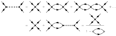
Figure 1: Diagrammatic representation of the RPA approximation.

In Ref. nosso1 the pseudo-scalar polarization loop and the $\pi_{0}$ pole mass have been calculated using the MFIR scheme. Next, we use the zMFIR regularization scheme to rewrite the expressions of the latter reference for the calculation of the $\pi_{0}$ pole mass. We start from the non-magnetized expression for the $\pi_{0}$ pole mass kleva :

$$m_{{\pi}^{0}}^{2}=-\frac{m}{M}\frac{1}{4GN_{c}N_{f}I(m_{\pi^{0}}^{2})}~{},$$ (53)

where in previous equation $k=(k_{0}=m_{\pi^{0}}^{2},\vec{k}=\vec{0})$ and

$$I(k^{2})=i\int\frac{d^{4}p}{(2\pi)^{4}}\frac{1}{[(p+\frac{k}{2})^{2}-M^{2}][(p-\frac{k}{2})^{2})-M^{2}]}\,.$$ (54)

Here, after using the Matsubara formalism in the latter integral, one obtains:

$$I(k_{0}^{2})=\int\frac{d^{3}p}{(2\pi)^{3}}\frac{1}{E(k_{0}^{2}-4E^{2})}(1-n(E)-\bar{n}(E))\,,$$ (55)

where the integration with respect to the variable $p_{0}$ was done by using the residue method PC1 . The magnetized version of the latter equation is obtained through the use of the prescription given in eq.(3) and it can be written as a sum of two terms, i. e., the vacuum and medium contribution:

$$I(k_{0}^{2})\rightarrow I(k_{0}^{2},B,T)~{}=~{}I_{vac}(k_{0}^{2},B)+I_{T,\mu}(k_{0}^{2},B)~{},$$ (56)

where

$$I_{vac}(k_{0}^{2},B) = \sum_{f=u,d}\beta_{f}\sum_{n=0}^{\infty}g_{n}\int_{-\infty}^{\infty}\frac{dp_{3}}{(2\pi)^{2}}$$ (57)

$$\times \frac{1}{4E_{n}\left(k_{0}^{2}-4E_{n}^{2}\right)}~{},$$

$$I_{T,\mu}(k_{0}^{2},B) = -\displaystyle{\sum_{f=u,d}\beta_{f}\sum_{n=0}^{\infty}g_{n}}\int_{-\infty}^{\infty}\frac{dp_{3}}{(2\pi)^{2}}$$ (58)

$$\times \frac{1}{4E_{n}\left(k_{0}^{2}-4E_{n}^{2}\right)}\left(n(E_{n})+\overline{n}(E_{n})\right)~{}.$$

The vacuum part of the previous expression was obtained in Ref. nosso1 using the MFIR scheme. It was shown that it can be separated in two terms, one the usual $B=0$ vacuum contribution and another due to the pure magnetic contribution:

$$I_{vac}(k_{0}^{2},B)=I_{vac}(k_{0}^{2})+I(k_{0}^{2},B)~{},$$ (59)

$$I_{vac}({k_{0}}^{2})=\int\frac{d^{3}p}{(2\pi)^{3}}\frac{1}{E\left(k_{0}^{2}-4E^{2}\right)}~{},$$ (60)

$$I(k_{0}^{2},B) = -\frac{\pi}{4(2\pi)^{3}}\sum_{f=u,d}\int^{1}_{0}dx\left[-\psi\left(\bar{x}_{f}+1\right)+\frac{1}{2\bar{x}_{f}}\right.$$ (61)

$$+ \left.\ln\bar{x}_{f}\right]~{},$$

where

$$\bar{x}_{f}=\frac{\overline{M}^{2}(k_{0}^{2})}{2\beta_{f}}~{}~{},~{}~{}\overline{M}^{2}(k_{0}^{2})=M^{2}-x(1-x)k_{0}^{2}~{}~{}$$

and $\psi(\bar{x}_{f})$ is the digamma function arfken . The usual ($B=0$) vacuum term, eq.(60), will be regularized through a 3D non-covariant cutoff. The expressions given in eqs.(53,58,59) can be used for the study of the neutral meson properties at finite $T$ e $\mu$. At the Mott temperature, i. e., when $k_{0}$=$m_{\pi^{0}}$ = $2M$ a singularity appears in the denominator and this pole has to be treated in a convenient way, since the pion becomes unstable and can decay in two quarks. It is possible to perform analytically the integration in eq.(60) obtaining for its real part the expression:

$$Re(I_{vac}(k_{0}^{2})) = -\frac{1}{8\pi^{2}}\left[\ln\frac{\Lambda+\epsilon_{\Lambda}}{\Lambda}\right.$$ (62)

$$- \theta(2M-k_{0})z_{0}~{}\tan^{-1}\left(\frac{\Lambda}{\epsilon_{\Lambda}z_{0}}\right)$$

$$- \left.\theta(k_{0}-2M)\frac{z_{0}}{2}\left(\ln\frac{\Lambda+\epsilon_{\Lambda}z_{0}}{\Lambda-\epsilon_{\Lambda}z_{0}}\right)\right],$$

with $z_{0}=\sqrt{|1-4M^{2}/k_{0}^{2}|}$. Analogously the real part of the magnetic vacuum term given in eq.(61) can also be calculated yielding:

$$Re(I(k_{0}^{2},B))=-\frac{1}{32\pi^{2}}\sum_{f=u,d}\left[-\int^{1}_{0}dx~{}\psi\left(\bar{x}_{f}+1\right)\right.$$

$$+\ln\frac{k_{0}^{2}}{2\beta_{f}}-2+\frac{2\beta_{f}}{k_{0}^{2}z_{0}}\ln\left|\frac{z_{0}-1}{z_{0}+1}\right|+$$

$$+~{}\theta(k_{0}-2M)\left(\ln\left|\frac{1-z_{0}^{2}}{4}\right|+z_{0}\ln\left|\frac{z_{0}+1}{z_{0}-1}\right|\right)+$$

$$\left.+~{}\theta(2M-k_{0})\left(\ln\left(\frac{1+z_{0}^{2}}{4}\right)+2z_{0}\tan^{-1}\frac{1}{z_{0}}\right)\right].$$ (63)

Notice that the latter expressions have a branch cut at $k_{0}=2M$ and they have to be interpreted as the Cauchy principal value when $k_{0}>2M$ flor . These two latter expressions extend our previous results for the pion mass calculation nosso1 including the regime where $k_{0}>2M$.

Next, we will return to the main focus of the present work ,i. e., to use the alternative zMFIR scheme in order to regularize the expressions for the polarization integral given in eqs.(57,58). From the eqs.(18,19,20) one obtains:

$$I(k_{0}^{2},B,T)=I_{vac}(k_{0}^{2})+I(k_{0}^{2},B)+I_{T,\mu}(k_{0}^{2})+I_{T,\mu}(k_{0}^{2},B)~{},$$ (64)

where

$$I_{vac}(k_{0}^{2}) = \sum_{f=u,d}\int_{M}^{\infty}dE\frac{E\sqrt{E^{2}-M^{2}}}{\pi^{2}}$$

$$\times \frac{1}{4E\left(k_{0}^{2}-4E^{2}\right)}~{},$$

$$I(k_{0}^{2},B) = \sum_{f=u,d}\frac{(2\beta_{f})^{1/2}}{2\pi^{2}}\int_{M}^{\infty}dEE(q_{E}){\cal H}_{1/2}(q_{E})$$

$$\times \frac{1}{4E(q_{E})\left(k_{0}^{2}-4E(q_{E})^{2}\right)}~{},$$

$$I_{T,\mu}(k_{0}^{2}) = -\sum_{f=u,d}\int_{M}^{\infty}dE\frac{E\sqrt{E^{2}-M^{2}}}{\pi^{2}}$$

$$\times \frac{n(E)+\bar{n}(E)}{4E\left(k_{0}^{2}-4E^{2}\right)}~{},$$

$$I_{T,\mu}(k_{0}^{2},B) = -\sum_{f=u,d}\frac{(2\beta_{f})^{1/2}}{2\pi^{2}}\int_{M}^{\infty}dEE(q_{E}){\cal H}_{1/2}(q_{E})$$

$$\times \frac{n(E(q_{E}))+\bar{n}(E(q_{E}))}{4E\left(k_{0}^{2}-4E(q_{E})^{2}\right)}~{}.$$

Therefore, we were able to separate exactly the magnetic and non-magnetic components of $I(k_{0}^{2},B,T)$ using the zMFIR regularization scheme. The only non finite contribution is the usual $B=0$ vacuum term $I_{vac}(k_{0}^{2})$. Performing the change of variables $p=\sqrt{E^{2}-M^{2}}$ in the latter expression for $I_{vac}(k_{0}^{2})$ one easily sees that we reobtain exactly the expression given in eq.(60) and as discussed above its regularized contribution is given by eq.(62). We perform the same change of variables in the non-magnetic medium term $I_{T,\mu}(k_{0}^{2})$ and it is straightforward to obtain:

$$I_{T,\mu}(k_{0}^{2})=\frac{1}{8\pi^{2}}\int_{0}^{\infty}dp\frac{p^{2}}{E(p^{2}-x_{0}^{2})}~{}(n(E)+\bar{n}(E))~{},$$ (65)

with $x_{0}^{2}=k_{0}^{2}/4-M^{2}$. Here, notice that when $x_{0}^{2}$ is greater than zero ($k_{0}>2M$) it is necessary to consider this integral as a Cauchy principal value. In order to obtain convenient expressions for the numerical calculation of the magnetic terms, we perform the change of variables:

$$x^{2}=q_{E}=\frac{E^{2}-M^{2}}{2\beta_{f}}~{}.$$

Thus, $dEE=2\beta_{f}~{}xdx$, $E=(2\beta_{f})^{1/2}\bar{E}_{f}$ with $\bar{E}_{f}=\sqrt{x_{f}+x^{2}}$ and $x_{f}\equiv\frac{M^{2}}{2\beta_{f}}$. It is straightforward to show that:

$$I(k_{0}^{2},B) = -\sum_{f=u,d}\frac{(2\beta_{f})^{1/2}}{32\pi^{2}}\int_{0}^{\infty}dxx{\cal H}_{1/2}(x^{2})$$ (66)

$$\times \frac{1}{{\bar{E}}_{f}\left(x^{2}-\bar{x}_{0}^{2}\right)}~{},$$

$$I_{T,\mu}(k_{0}^{2},B) = \sum_{f=u,d}\frac{(2\beta_{f})^{1/2}}{32\pi^{2}}\int_{0}^{\infty}dxx{\cal H}_{1/2}(x^{2})$$ (67)

$$\times \frac{n(E)+\bar{n}(E)}{{\bar{E}}_{f}\left(x^{2}-\bar{x}_{0}^{2}\right)}~{},$$

where $\bar{x}_{0}^{2}=(k_{0}^{2}/4-M^{2})/(2\beta_{f})$. Of course, the latter expressions also have to be interpreted as Cauchy principal values when $\bar{x}_{0}^{2}$ is greater than zero or, equivalently, when $k_{0}>2M$, i. e., the Mott temperature is univocally defined when the system is immersed in a magnetic medium. The $\pi_{0}$ pole mass is calculated numerically using the eqs.(53,64) in terms of the Hurwitz-Riemann zeta functions as discussed above and our results will be presented in the next section.

IV Numerical Results

In the following we present the numerical results. The set of parameters utilized for the $3$D cutoff regularization are $\Lambda=664.3$ MeV, $m_{0}=5.0$ MeV and $G=\frac{2.06}{\Lambda^{2}}$ buballa . Firstly, we sketch in Fig. 2 the effective quarks masses as well as the pole-mass of neutral meson $\pi_{0}$ at finite temperature and zero magnetic field. At low temperatures the effective quark mass is almost the same as calculated in the vacuum, i.e, $M(T)\approx M(0)$, as well as the pole-mass of the $\pi^{0}$ meson. When the pseudo-critical temperature is exceeded, the chiral symmetry is partially restored and the effective quark mass becomes almost the current quark masses $M\approx m_{0}$. The Mott dissociation happens when the system gets $m_{\pi}(T)=2M(T)$ blasche at $T_{Mott}=179.8$ MeV. In the Wigner-Weyl phase, the equations (55) should be interpreted as its Principal Value, due to the divergences in the denominator when $p=\sqrt{\frac{m_{\pi^{0}}^{2}}{4}-M^{2}}$ flor ; asakawa .

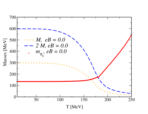
Figure 2: Masses as a function of the temperature for eB=0.

The behavior of the effective quark masses at finite temperature at $eB=0.1$GeV² can be seen in panel (a) in the Fig. 3. As in the previous case, the pole-mass of the neutral collective excitation is showed in the same figure as well. For the effective quark masses evaluated in both formalisms in the present paper, i.e., eq(42) and eq(44), almost no difference can be seen in the numerical results as we already mentioned and the well known behavior is sketched. At low temperatures, the magnetic field enhances the breaking of the chiral symmetry and the effective quark masses becomes more stronger (magnetic catalysis revigor ). When the temperature is greater than the pseudo-critical temperature, the chiral symmetry partially restores, and the effective quark masses becomes weaker. For completeness, we mention that in this scenario, it is well established that the pseudo-critical temperature $T_{c}$ increases with $eB$ farias ; farias2 .

For the pole-masse of the neutral collective excitation, the analysis becomes more complicated. For low temperatures($T<T_{c}$) the behavior of the neutral meson is almost as expected, the $m_{\pi^{0}}(B,T)\approx m_{\pi^{0}}(B)$. We can understand this in terms of the chiral symmetry restoration. In this phase, these mesons are protected by the Goldstone phase, and the magnetic field is strengthening the break of the partially chiral symmetry. When the temperature is sufficiently to partially restore the chiral symmetry, the neutral mesons enters in the Wigner-Weyl phase. In this phase, the $\pi_{0}$ meson is a thermal excitation with a finite decay width, but the increase of the magnetic field causes the thermal excitations to become more energetic when compared with the zero magnetic field case. The $\pi^{0}$ mass suddenly jumps to a more energetic solution at the dissociation temperature. Following the previous analysis, for the $eB=0.1$GeV², we found $T_{Mott}=195$ MeV.

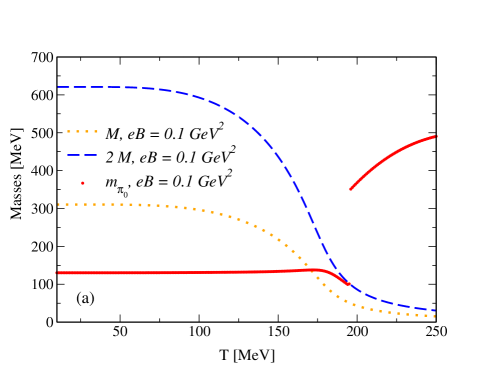
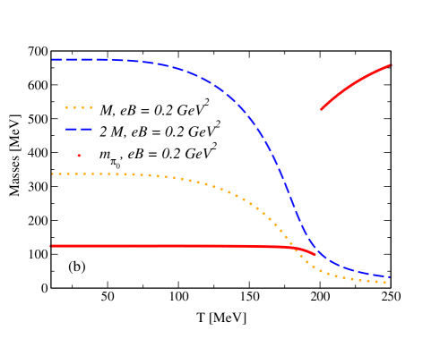
Figure 3: Masses as a function of the temperature for different values of magnetic field.

In panel (b) of Fig 3 we sketch the results with $eB=0.2\,GeV^{2}$, and as expected, at low temperatures the previous analysis can still be used, where we have $m_{\pi^{0}}(B,T)\approx m_{\pi^{0}}(B)$. The interpretation slightly changes if we look beyond the Mott Temperature $T_{Mott}=200.2$ MeV, where the magnetic field enhances the resonant excitations to more energetic states. We show that using zMFIR regularization scheme that the effect of the magnetic field is catalyze the Mott temperature, result that is the opposite found in recent literature mao . Other point in Ref. mao that is not clear is the position of the jump on the pion mass, the authors claim that the jump happens in the Mott temperature, but we do not observe this in Fig.2 of Ref. mao , e.g. the jump for eB $=10\,m_{\pi}^{2}$ happens when $m_{\pi}=M$, and the definition for Mott temperature is $m_{\pi}=2M$.

IV.1 The nature of the sudden jump on the pion mass

In mao the author use Pauli-Villars regularization in NJL model to study the behavior of the neutral pion mass as a function of the temperature for different values of magnetic fields. The author presents a good explanation for the sudden jump on the pion mass at the Mott temperature, he argued that these more energetic thermal excitations appear due the divergence at the Lowest Landau Level (LLL) that is associated with the dimensional reduction caused by the strong magnetic fields.

The dimensional reduction of fermionic systems at strong magnetic field has been explored by several authors gus ; fukushima2 and plays a fundamental role to explain these more energetic resonances. In the MFIR formalism we can clearly see in a more transparent way that we have a physical dimensional reduction of our system when we compare with the $eB=0$ equations. The LLL dominance at strong magnetic field makes our system go in a naively way to $3+1$ D$\,\,\rightarrow\,\,1+1$ D, e.g., see eq.(31) when $n\rightarrow 0$ in comparison with eq.(29). But, if our system is going to the high temperature limit, the highest Landau Levels become populated again, because of the weakening of the interaction of the fermions in the chiral condensate.

For the collective excitations, the idea becomes the same. The high temperature($T>T_{Mott}$) is not sufficient to excite all possible states in the phase space, as we have in the $eB=0$ case, that allow the resonant pair $q-\bar{q}$ to occupy. Due to the dimensional reduction associated with the magnetic field, the number of states for the excited pair is reduced, and the momentum integration is not sufficiently to guarantee some solution to the resonant state of the $\pi^{0}$ at energy states right after $m_{\pi^{0}}\approx 2M$. That is, the dimensional reduction of the system enforces the system to have less states than the $eB=0$ case. On the other hand, the condition $1-2G\Pi_{ps}(k_{0}^{2}=m_{\pi^{0}}^{2})=0$ is the RPA equation for the pole-mass, that ensures to us that the conservation of the external momenta in the RPA bubbles should be on shell. Therefore, we can expect that the $\pi^{0}$ mass jump to another more energetic state at the Mott Temperature. This jump is just the $\pi^{0}$ mass going to its lowest possible energy state, when all other states are not accessible anymore.

At the Wigner-Weyl phase, we should mention an interesting phenomenon. If we look at the top of figure 3, we can see a decrease of the energy of the resonant $\overline{q}-q$ state (or the $\pi_{0}$ mass) at finite magnetic field $eB=0.1$GeV ² and high temperature(say $T=250$ MeV) when compared to the same situation at $eB=0$ of the figure 2. On the other hand, if we increase the magnetic field (in our case we see this for $eB=0.2$ GeV² at the bottom of the figure 3), the energy of the resonant state increases above the $eB=0$ situation and this effect can be understood as an oscillatory behavior. The main reason for this to happen is that at $eB=0$ most of the energy of the neutral resonance is generated thermally. At finite magnetic field the dimensional reduction that takes place softens the thermal energy. At a certain small magnetic field the dimensional reduction and the magnitude of the magnetic field are not sufficiently strong to increase the energy of the resonant pair above the energy associated with $eB=0$ case. If we increase the magnetic field to $eB=0.2$ GeV²(as we see in the fig.3), we will have more energy from the magnetic field contributing to the resonant $\overline{q}-q$ pair overcoming at a certain point the weakening due to the dimensional reduction, increasing for this reason the energy of the state.

V Effects due inverse magnetic catalysis

Inverse magnetic catalysis is a remarkable phenomena that was discovered by lattice QCD simulations bali ; lattice . Recently was shown that IMC can be reproduced in Nambu–Jona-Lasinio model if thermo-magnetic effects are include in the coupling constant $G(eB,T)$ farias ; farias2

In order to see how the inverse magnetic catalysis can influence our results, we improve the calculations using the same $G(eB,T)$ fitted to the lattice data for the average of the quark condensates bali . In farias2 this fit was obtained by using the following interpolation formula for $G(eB,T)$:

$$G(B,T)=c(B)\left[1-\frac{1}{1+e^{\beta(B)\left[T_{a}(B)-T\right]}}\right]+s(B).$$ (68)

The values of the parameters $c,s,\beta$ and $T_{a}$ are shown in Table 2 and for the the parametrization of the model we take standard values, $\Lambda=0.650~{}{\rm GeV}$ and $m=5.5~{}{\rm MeV}$.

Table 2: Values of the fitting parameters in Eq. (68). Units are in appropriate powers of GeV.

$eB$	$c$	$T_{a}$	$s$	$\beta$
0.0	0.900	0.168	3.731	40.000
0.2	1.226	0.168	3.262	34.117
0.4	1.769	0.169	2.294	22.988
0.6	0.741	0.156	2.864	14.401
0.8	1.289	0.158	1.804	11.506

In the Fig. 4 we show the effect of the inverse magnetic catalysis in the effective quark masses as well as the pole-mass of the neutral meson. The Mott temperature in this case suffers a inverse magnetic catalysis in the same way, passing by $T_{Mott}=166.84$ MeV at $eB=0.1$ GeV² to $T_{Mott}=164.9$ MeV at $eB=0.2$ GeV². The resonances as we can see are still more energetic as we grow the magnetic field.

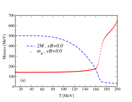
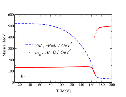
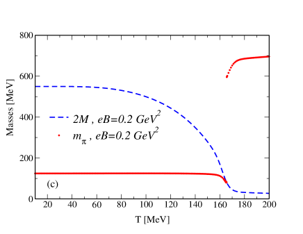
Figure 4: Masses as a function of the temperature for different values of magnetic field using the thermo-magnetic dependence on the coupling constant $G(eB,T)$.

The physical analysis involving the chiral symmetry restoration at strong magnetic fields is the same as the one discussed in the previous section. The magnetic field enhances the binding of the condensate and the broken chiral symmetry is even more evident. As we increase the temperature the weakening of the chiral condensate happens and the chiral symmetry can be partially restored at high temperatures. At this point, the difference from our previous section is that the coupling constant $G$ is substituted by a thermo-magnetic dependent coupling $G\rightarrow G(eB,T)$ that mimics the inverse magnetic catalysis in our results for the effective quark masses. For the neutral meson mass the broken chiral symmetry preserves at low temperature $m_{\pi^{0}}(B,T)\approx m_{\pi^{0}}(B,0)$ the pole mass approximately as a pseudo-Goldstone boson. If we increase the temperature with the coupling $G(eB,T)$ our results show that the Mott temperature decreases compared to the constant coupling $G$ case, in agreement with what is expected by the inverse magnetic catalysis. The oscillatory behavior in the Wigner-Weyl phase, illustrated in the last section, also occurs in the present case as we can see from the results of the figure 4. The physical analysis of this behavior is the same as pointed out in the last section, since we have just modified the field dependent coupling $G(eB,T)$.

However, we should pay attention to the fact that the physical mechanism behind the inverse magnetic catalysis (IMC) is still under debate, for more discussions revigor .

Also, we have to mention that, some works evaluating the neutral mesons masses at finite magnetic fields and temperatures have not obtaining any jump in the $\pi^{0}$ pole-mass at the dissociation temperature, and this can cause some misunderstanding. As explained in zhuang ; iran , there are some approximations in the formalism, an special is the integral $I(k_{0}^{2})\approx I(0)$. Another feature that can be explored is the role of the regularizations that are used and are not fully exploited, since the choice of some regularizations can produce significant non-physical results norberto ; ricardo ; scoccola , differently of the case of the regularization adopted in this work.

VI Conclusions

In this work we have presented a study of the NJL SU(2) at finite temperatures and magnetic fields in the MFIR scheme. In an analogous way, we show an equivalent and helpful formalism that we call zMFIR, applicable in future several applications.

The new formalism presented in this work has the advantage of separating in an exact way the magnetic from non-magnetic contributions for the expressions of physical interest, i. e., the thermodynamic potential, gap equation, polarization loops, etc. As an example of a direct application of the zMFIR, we expand the formalism for the RPA framework, and we evaluate the pole-mass of $\pi^{0}$ meson at finite magnetic field and temperatures. Again, both formalisms agree almost exactly in their numerical results, though the zMFIR showed to be more efficient to work in the numerical evaluations. The first dramatic result is the more energetic resonances that we obtain as we increase the magnetic field. As we explained, this is a direct result from the dimensional reduction of the system at strong magnetic fields that enforces the system to go to another state, since we have less states to the creation of the thermal $q-\bar{q}$ excitation.

As mentioned in norberto ; ricardo ; scoccola , the MFIR scheme avoid some unphysical results, and this choice of regularization provide to us some different results from most of the regularizations prescriptions of the current literature. The Mott dissociation temperature is catalyzed with the increase of the magnetic field as well as the pseudo-critical temperature. This behavior of the Mott temperature goes in a inverse way of the reference mao . We believe that some differences associated with the regularization adopted in that work can be affecting the way the mesons are becoming resonances. Also, the fact that we are working in a mean field approximation strengthens the idea that in this approximation, we have to see the catalyzed Mott Temperature.

To recover the expected result from Lattice bali we also employed the $G(eB,T)$ from farias2 . The inverse magnetic catalysis in the NJL SU(2) model as discussed in the main text is recovered, and in the same way we obtain a inverse magnetic catalysis of the Mott Temperature.

As a suplementary result, the magnetic vacuum polarization integral of referencenosso1 has been extended by using the analytic continuation technique. These analytical expressions are useful for the validation of more complicated numerical calculations.

Appendix A regularization of the magnetic effective potential term

Next, we will discuss how to identify and separate the divergent contribution to the vacuum magnetic effective potential term $\tilde{\Omega}_{vac}(B)$. This latter term can be obtained by substituting the explicit form of $\tilde{g}_{f}(q_{E},B)$, eq.(22), in eq.(34):

$$\tilde{\Omega}_{vac}(B)=-N_{c}\sum_{f=u,d}\frac{(2\beta_{f})^{2}}{(2\pi)^{2}}\int_{0}^{\infty}dq_{E}\sqrt{x_{f}+q_{E}}$$

$$\times\left[\zeta(\frac{1}{2},\{q_{E}\})-\left(\zeta(\frac{1}{2},q_{E})+2q_{E}^{1/2}-\frac{1}{2q_{E}^{1/2}}\right)\right]~{},$$ (69)

where $x_{f}=\frac{M_{f}^{2}}{2\beta_{f}}$. From the asymptotic limit of the zeta function $\zeta(1/2,q_{E})$ DE ,

$$\zeta(\frac{1}{2},q_{E})=-2q_{E}^{1/2}+\frac{1}{2q_{E}^{1/2}}+\frac{1}{24}q_{E}^{-3/2}+O(q_{E}^{-7/2})~{}~{},$$ (70)

we see that the integrand in eq.(69) is logarithmically divergent. Hence, we will sum and subtract the term $-\frac{1}{24}q_{E}^{-3/2}$ in the integrand, since this term forces the convergence of the integral. Therefore, one obtains:

$$\tilde{\Omega}_{vac}(B)=-N_{c}\sum_{f=u,d}\frac{(2\beta_{f})^{2}}{(2\pi)^{2}}\left[\frac{}{}\right.$$

$$-\int_{0}^{\infty}dq_{E}\frac{\sqrt{x_{f}+q_{E}}}{24q_{E}^{3/2}}+\int_{0}^{\infty}dq_{E}\zeta(\frac{1}{2},\{q_{E}\})\sqrt{x_{f}+q_{E}}$$

$$\left.-\int_{0}^{\infty}dq_{E}\left(\zeta(\frac{1}{2},q_{E})+2q_{E}^{1/2}-\frac{1}{2q_{E}^{1/2}}-\frac{1}{24q_{E}^{3/2}}\right)\sqrt{x_{f}+q_{E}}\right].$$

(71)

The first integration in the latter equation is trivial :

$$\int_{0}^{\infty}dq_{E}\frac{\sqrt{x_{f}+q_{E}}}{q_{E}^{3/2}}=\left.-2\left(\frac{\sqrt{x_{f}+q_{E}}}{q_{E}^{1/2}}+\ln[q_{E}^{1/2}+\sqrt{x_{f}+q_{E}}]\right)\right|_{0}^{\infty}~{}.$$ (72)

The integral involving the periodic function, $\zeta(\frac{1}{2},\{q_{E}\})$, in eq.(71) can be rewritten by noting that:

$$\int_{0}^{\infty}dxf(x)g(x)=\int_{0}^{1}dxf(x)g(x)+\int_{1}^{2}dxf(x)g(x)$$

$$+\int_{2}^{3}dxf(x)g(x)+\dots=\int_{0}^{1}dxf(x)\sum_{k=0}^{\infty}g(x+k)~{},$$ (73)

where f(x) is a periodic function with period 1 and g(x) an arbitrary function. Notice that a change of variables was done to set the limits of integration of all integrals from 0 to 1. Then, it follows that:

$$\int_{0}^{\infty}dq_{E}\zeta(\frac{1}{2},\{q_{E}\})\sqrt{x_{f}+q_{E}}=$$

$$\int_{0}^{1}dq_{E}\zeta(\frac{1}{2},q_{E})\sum_{k=0}^{\infty}\sqrt{x_{f}+q_{E}+k}~{}.$$ (74)

From the definition of the Hurwitz-Riemann zeta function, eq.(10), the latter integral may be written as:

$$\int_{0}^{1}dq_{E}\zeta(\frac{1}{2},\{q_{E}\})\sum_{k=0}^{\infty}\sqrt{x_{f}+q_{E}+k}~{}$$

$$=\int_{0}^{1}dq_{E}~{}\zeta(\frac{1}{2},q_{E})~{}\zeta(-\frac{1}{2},x_{f}+q_{E})~{}.$$ (75)

At this point, we substitute eqs.(72,75) in eq.(71). Finally, aiming a more suitable expression for numerical calculations, we use the following property of the Riemann-Hurwitz zeta function apostol

$$\frac{\partial}{\partial y}\zeta(z,y)=-z\zeta(z+1,y)~{},$$ (76)

in order to perform an integration by parts in eq.(71). Then, the final regularized finite magnetic vacuum term is given by:

$$\tilde{\Omega}_{vac}(B) = -N_{c}\sum_{f=u,d}\frac{(2\beta_{f})^{2}}{(2\pi)^{2}}~{}\left\{\frac{2}{24}+\frac{1}{24}\ln x_{f}\right.$$ (77)

$$- \int_{0}^{1}dq_{E}\zeta(-\frac{1}{2},\{q_{E}\})\zeta(\frac{1}{2},q_{E}+x_{f})$$

$$+ \int_{0}^{\infty}dq_{E}\left[\zeta(-\frac{1}{2},q_{E})+\frac{2}{3}q_{E}^{3/2}\right.$$

$$- \left.\left.\frac{1}{2}q_{E}^{1/2}+\frac{1}{24}q_{E}^{-1/2}\right]\frac{1}{\sqrt{x_{f}+q_{E}}}\right\}~{}.$$

This integral is adequate for numerical calculations and we have discarded all the unphysical divergent terms. As discussed in section II.A, the latter regularized magnetic vacuum expression numerically coincides with the one obtained by using other formalisms.

Appendix B the equivalence between MFIR and zMFIR

Here, we will present the main steps for proving the equivalence between the zMFIR and MFIR formalisms for obtaining the gap equation.

Starting from eq.(43) at $T=0$:

$$\frac{M-m}{2MG}=~{}I_{G}+I_{G}(B)~{},$$ (78)

where $I_{G}$ is the vacuum contribution and $I_{G}(B)$ is given by:

$$I_{G}(B)=N_{c}\sum_{f=u,d}\int_{0}^{\infty}~{}dq_{E}~{}~{}\frac{(2\beta_{f})^{3/2}}{(2\pi)^{2}}\frac{\tilde{\cal H}_{1/2}(q_{E})}{E(q_{E})}~{}$$ (79)

and $E(q_{E})$ and $\tilde{\cal H}_{1/2}(q_{E})$ are given in eqs.(21,23) respectively. We can split eq.(79) in two contributions:

$$I_{G}(B)=N_{c}\sum_{f=u,d}\left[I(x_{f})_{z}+I(x_{f})_{div}\right],$$ (80)

in the last equation:

$$I(x_{f})_{z} = \frac{(2\beta_{f})}{(2\pi)^{2}}\int_{0}^{\infty}~{}dq_{E}~{}~{}\frac{\left(\zeta(\frac{1}{2},\{q_{E}\})-\zeta(\frac{1}{2},q_{E})\right)}{(x_{f}+q_{E})^{1/2}},$$ (81)

$$I(x_{f})_{div} = \frac{(2\beta_{f})}{(2\pi)^{2}}\int_{0}^{\infty}~{}dq_{E}~{}~{}\frac{\left(-2q_{E}^{1/2}+\frac{1}{2q_{E}^{1/2}}\right)}{(x_{f}+q_{E})^{1/2}}.$$ (82)

These two integrals can be evaluated by using an integration by parts and the eq.(76), yielding

$$I(x_{f})_{z} = \frac{(2\beta_{f})}{(2\pi)^{2}}\int_{0}^{\infty}dq_{E}\frac{\left(\zeta(-\frac{1}{2},\{q_{E}\})-\zeta(-\frac{1}{2},q_{E})\right)}{(x_{f}+q_{E})^{3/2}},$$ (83)

$$I(x_{f})_{div} = \frac{(2\beta_{f})}{(2\pi)^{2}}\int_{0}^{\infty}dq_{E}\frac{\left(-\frac{2}{3}q_{E}^{3/2}+\frac{q_{E}^{1/2}}{2}\right)}{(x_{f}+q_{E})^{3/2}}.$$ (84)

Next, we use the same procedure of Appendix A in order to rewrite the first of these two integrals. First, we use eq.(73) to obtain:

$$\int_{0}^{\infty}dq_{E}\zeta(-\frac{1}{2},\{q_{E}\})\frac{1}{(x_{f}+q_{E})^{3/2}}=$$

$$\int_{0}^{1}dq_{E}\zeta(-\frac{1}{2},q_{E})\sum_{k=0}^{\infty}\frac{1}{(x_{f}+q_{E})^{3/2}}~{}.$$ (85)

From the definition of the Hurwitz-Riemann zeta function, eq.(10), the last sum of integrals may be written as:

$$\int_{0}^{1}dq_{E}\zeta(-\frac{1}{2},\{q_{E}\})\sum_{k=0}^{\infty}\frac{1}{(x_{f}+q_{E})^{3/2}}~{}$$

$$=\int_{0}^{1}dq_{E}~{}\zeta(-\frac{1}{2},q_{E})~{}\zeta(\frac{3}{2},x_{f}+q_{E})~{}.$$ (86)

Returning to eq.(83), we can rewrite $I(x_{f})_{z}$:

$$I(x_{f})_{z} = \frac{(2\beta_{f})}{(2\pi)^{2}}\left(\int_{0}^{1}~{}dq_{E}~{}~{}\zeta(-\frac{1}{2},q_{E})\zeta(\frac{3}{2},x_{f}+q_{E})\right.$$ (87)

$$- \left.\int_{0}^{\infty}~{}dq_{E}\frac{\zeta(-\frac{1}{2},q_{E})}{(x_{f}+q_{E})^{3/2}}\right).$$

We will now make use of the following mathematical identities(all of them are valid for $q_{E}>1$)apostol2 :

$$\zeta(\frac{3}{2},x_{f}+q_{E}) = \frac{1}{\Gamma(3/2)}\int_{0}^{\infty}dy\frac{y^{1/2}e^{-y(x_{f}+q_{E})}}{1-e^{-y}},$$ (88)

$$\zeta(-\frac{1}{2},q_{E}) = \frac{\Gamma(3/2)}{2\pi i}\int_{\mathcal{C}}dz\frac{z^{-3/2}e^{zq_{E}}}{1-e^{z}},$$ (89)

$$\frac{1}{(x_{f}+q_{E})^{3/2}} = \frac{1}{\Gamma(3/2)}\int_{0}^{\infty}dyy^{1/2}e^{-y(q_{E}+x_{f})},$$ (90)

where the integral in identity eq.(89) is defined over the Hankel contour $\mathcal{C}$. Applying these identities to eq.(87), we can perform the integrations with respect to $q_{E}$ getting the result:

$$I(x_{f})_{z}=\frac{(2\beta_{f})}{(2\pi)^{2}}\frac{1}{2\pi i}\int_{0}^{\infty}dy\frac{y^{-1/2}e^{-yx_{f}}}{e^{y}-1}\int_{\mathcal{C}}dz\frac{z^{-3/2}}{1-\frac{z}{y}}.$$ (91)

On the contour $\mathcal{C}$ we will use the parametrizations $z=re^{-i\pi}$ below the negative real axis and $z=re^{i\pi}$ above the real axis with $0<r<\infty$. As the first argument of the Riemann-Hurwitz zeta function eq.(89) is negative, we can explore its analytic continuation. With these definitions, one obtains for the contour integration:

$$\int_{\mathcal{C}}dz\frac{z^{-3/2}}{1-\frac{z}{y}} =-\int_{0}^{\infty}dre^{-i\pi}(e^{-i\pi}r)^{-3/2}(1-\frac{e^{-i\pi}r}{y})^{-1}$$ (92)

$$+\int_{0}^{\infty}dre^{i\pi}(e^{i\pi}r)^{-3/2}(1-\frac{e^{i\pi}z}{y})^{-1},$$

$$=2i\sin(-\frac{\pi}{2})y^{-1/2}B(-1/2,3/2),$$

where $B(a,b)$ is the Beta function apostol given by

$$B(a,b)=\int_{0}^{\infty}t^{a-1}(1+t)^{-a-b}~{}.$$ (93)

where the latter expression can be written in terms of gamma functions as $B(a,b)=\frac{\Gamma(a)\Gamma(b)}{\Gamma(a+b)}$. Afterwards, using the results of eqs.(92,93) in eq.(91), one obtains:

$$I(x_{f})_{z}=\frac{(2\beta_{f})}{(2\pi)^{2}}\int_{0}^{\infty}dy\frac{e^{-yx_{f}}y^{-1}}{e^{y}-1}.$$ (94)

This quantity diverges at the origin. We can use the series expansion $\frac{1}{e^{y}-1}\approx\frac{1}{y}-\frac{1}{2}+\mathcal{O}(y)$ to separate the divergent part of the latter expression. By adding and subtracting the first terms of the series in eq.(94) one obtains:

$$I(x_{f})_{z} = \frac{(2\beta_{f})}{(2\pi)^{2}}\int_{0}^{\infty}dy\frac{e^{-yx_{f}}}{y}\left(\frac{1}{e^{y}-1}-\frac{1}{y}+\frac{1}{2}\right)$$ (95)

$$+ \frac{(2\beta_{f})}{(2\pi)^{2}}\left(\int_{0}^{\infty}dy\frac{e^{-yx_{f}}}{y^{2}}-\int_{0}^{\infty}dy\frac{e^{-yx_{f}}}{2y}\right).$$

The quantity $I(x_{f})_{div}$ cancels out the last two integrals in eq.(95). This can be seen using the identity, eq.(90), in $I(x_{f})_{div}$. Noticing that $\frac{1}{e^{y}-1}=-\frac{1}{2}+\frac{1}{2}\coth\left(\frac{y}{2}\right)$ and performing the change of variables $\frac{y}{2\beta_{f}}=\mu\rightarrow\frac{y}{2\beta_{f}}=d\mu$, we can rewrite eq.(80) as:

$$I_{G}(B)=N_{c}\sum_{f=u,d}\left[I(x_{f})_{z}+I(x_{f})_{div}\right],$$

$$=N_{c}\sum_{f=u,d}\frac{\beta_{f}}{(2\pi)^{2}}\int_{0}^{\infty}d\mu\frac{e^{-\mu M_{f}^{2}}}{\mu^{2}}\left(\mu\coth\left(\beta_{f}\mu\right)-\frac{1}{\beta_{f}}\right).$$

$$=N_{c}\sum_{f=u,d}\frac{\beta_{f}}{2\pi^{2}}\left[\log\Gamma(x_{f})-(x_{f}-\frac{1}{2})\log(2\pi)+\right.$$

$$\left.x_{f}-\frac{1}{2}\log 2\pi\right].$$

If we substitute the last result in eq.(78), the usual expression for the gap equation calculated within the MFIR schemenosso2 will be reobtained.

References

- (1) K. Fukushima, D. E. Kharzeev and H. J. Warringa, Phys. Rev. D 78, 074033 (2008); D. E. Kharzeev and H. J. Warringa, Phys. Rev. D 80, 034028 (2009); D. E. Kharzeev, Nucl. Phys. A 830, 543c (2009).
- (2) V. Skokov, A. Yu. Illarionov, and V. Toneev, Int. J. Mod. Phys. A 24, 5925 (2009).
- (3) A. Bzdak and V. Skokov, Phys. Lett. B 710, 171 (2012).
- (4) L. Ou and B. -A. Li, Phys. Rev. C 84, 064605 (2011).
- (5) V. Voronyuk, V. D. Toneev, W. Cassing, E. L. Bratkovskaya, V. P. Konchakovski, and S. A. Voloshin, Phys. Rev. C 83, 054911 (2011).
- (6) R. Duncan and C. Thompson, Astron. J., 392, L9 (1992).
- (7) C. Kouveliotou et al., Nature 393, 235 (1998).
- (8) G. S. Bali, B. B. Brandt, G. Endrődi and B. Glässle, Phys. Rev. Lett. 121, 072001 (2018).
- (9) Sh. Fayazbakhsh and N. Sadooghi, Phys. Rev. D 88, 065030 (2013).
- (10) Yu. A. Simonov, Phys. At. Nucl. 79, 455 (2016).
- (11) S. Ghosh, Arghya Mukherjee, M. Mandal, S. Sarkar, and P. Roy, Phys. Rev. D 94, 094043 (2016).
- (12) A. Bandyopadhyay, S. Mallik, Eur. Phys. J. C 77 ,771 (2017).
- (13) R. M. Aguirre, arXiv:1808.04404 [nucl-th].
- (14) T. Yoshida and K. Suzuki, Phys. Rev. D 94, 074043 (2016).
- (15) D. Dudal and T. G. Mertens, Phys. Rev. D 91, 086002 (2015).
- (16) Kevin Marasinghe and Kirill Tuchin, Phys. Rev. C 84, 044908 (2011).
- (17) P. Gubler, K. Hattori, S. H. Lee, M. Oka, S. Ozaki, and K. Suzuki, Phys. Rev. D 93, 054026 (2016).
- (18) C. S. Machado, S. I. Finazzo, R. D. Matheus, and J. Noronha, Phys. Rev. D 89, 074027 (2014).
- (19) S. Cho, K. Hattori, S. H. Lee, K. Morita, and S. Ozaki, Phys. Rev. Lett. 113, 172301 (2014).
- (20) S. Cho, K. Hattori, S. H. Lee, K. Morita, and S. Ozaki, Phys. Rev. D 91, 045025 (2015).
- (21) S. S. Avancini, W. R. Tavares and M. B. Pinto, Phys. Rev. D 93, 014010 (2016).
- (22) S. S. Avancini, R. L. Farias, M. B. Pinto, W. R. Tavares and V. S. Timteo, Phys. Lett. B 767, 247 (2017).
- (23) Z. Wang and P. Zhuang, Phys. Rev. D 97, 034026 (2018).
- (24) Sh. Fayazbakhsh, S. Sadeghian, and N. Sadooghi, Phys. Rev. D 86, 085042 (2012).
- (25) M. Coppola, D. Gómez Dumm, N. N. Scoccola, Phys. Lett. B 782, 155 (2018).
- (26) H. Liu, X. Wang, L. Yu and M. Huang, Phys. Rev. D 97, 076008 (2018).
- (27) D. Gómez Dumm, M. F. Izzo Villafañe, and N.N. Scoccola, Phys. Rev. D 97, 034025 (2018).
- (28) M. A. Andreichikov, B. O. Kerbikov, E. V. Luschevskaya, Yu. A. Simonov and O.E.Solovjeva, JHEP, 1705, 007 (2017).
- (29) Alejandro Ayala, Ricardo L. S. Farias, S. Hernandez-Ortiz, Luis A. Hernandez, D. Manreza Paret, R. Zamora, arXiv:1809.08312 [hep-ph].
- (30) S. Mao, arXiv:1808.10242 [nucl-th].
- (31) A. Mukherjee, S. Ghosh, M. Mandal, P. Roy, and S. Sarkar, Phys. Rev. D 96, 016024 (2017).
- (32) S. Ghosh, A. Mukherjee, M. Mandal, S. Sarkar, and P. Roy, Phys. Rev. D 96, 116020 (2017).
- (33) R. Zhang, W.-j. Fu, and Y.-x. Liu, Eur. Phys. J. C 76 307 (2016).
- (34) H. Liu, L. Yu, and M. Huang, Phys. Rev. D 91, 014017 (2015).
- (35) M. A. Andreichikov, Yu. A. Simonov, arXiv:1805.11896 [hep-ph].
- (36) G. Colucci, E .S. Fraga and A. Sedrakian, Phys. Lett. B 728, 19 (2014)
- (37) R. M. Aguirre Phys. Rev. D 96, 096013 (2017).
- (38) H. Taya, Phys. Rev. D 92, 014038 (2015).
- (39) M. Kawaguchi and S. Matsuzaki, Phys. Rev. D 93, 125027(2016).
- (40) J. O. Andersen, Phys. Rev. D 86, 025020 (2012).
- (41) K. Hattori, T. Kojo, and N. Su, Nucl. Phys. A 951, 1 (2016), arXiv:1512.07361 [hep-ph].
- (42) M. A. Andreichikov, B. O. Kerbikov, V. D. Orlovsky, and Yu. A. Simonov, Phys. Rev. D 87, 094029 (2013).
- (43) N. Callebaut, D. Dudal and H. Verschelde, JHEP 1303, 033 (2013).
- (44) N. Callebaut and D. Dudal, JHEP 1401, 055 (2014).
- (45) G. S. Bali, B. B. Brandt, G. Endrödi, and B. Glőssle, Phys. Rev. D 97, 034505 (2018).
- (46) G. Bali, B.B. Brandt, G. Endrödi, and B. Glőssle, PoS LATTICE 2015, 265 (2016). arXiv:1510.03899 [hep-lat].
- (47) E. V. Luschevskaya, O.E. Solovjeva, O. E. Kochetkov and O. V. Teryaev, Nucl. Phys. B 898, 627, (2015).
- (48) E. V. Luschevskaya, O. E. Kochetkov, O. V.Larina and O. V. Teryaev, Nucl. Phys. B 884, 1 (2014).
- (49) E.V. Luschevskaya, O.E. Solovjeva, and O.V. Teryaev, Phys. Lett. B 761, 393 (2016).
- (50) Y. Hidaka and A. Yamamoto, Phys. Rev. D 87, 094502 (2013).
- (51) M. A. Andreichikov, B. O. Kerbikov, V. D. Orlovsky, and Yu. A. Simonov, Phys. Rev. D 89, 074033 (2014).
- (52) B.-R. He, Phys. Rev. D 92, 111503 (2015).
- (53) P. G. Allen, A. G. Grunfeld and N. N. Scoccola, Phys. Rev. D 92, 074041 (2015).
- (54) D.C. Duarte, P. G. Allen, R.L.S. Farias, P.H.A. Manso, R.O. Ramos, and N. N. Scoccola, Phys. Rev. D 93, 025017 (2016).
- (55) D. Ebert and K. G. Klimenko, Nucl. Phys. A 728, 203 (2003).
- (56) D. P. Menezes, M. B. Pinto, S. S. Avancini, A. Pérez Martínez and C. Providência, Phys. Rev. C 79, 035807 (2009).
- (57) C. O. Dib and O. Espinosa, Nucl. Phys. B 612, 492 (2001).
- (58) Bo Feng, De-fu Hou and Hai-cang Ren, Phys. Rev. D 92, 065011 (2015).
- (59) Bo Feng, De-fu Hou, Hai-cang Ren and Ping-ping Wu, Phys. Rev. D 93, 085019 (2016).
- (60) R. L. S. Farias, K. P. Gomes, G. Krein, and M. B. Pinto, Phys. Rev. C 90, 025203 (2014).
- (61) R.L.S. Farias, V.S. Timóteo, S.S. Avancini, M.B. Pinto, G. Krein , Eur. Phys. J. A 53, 101 (2017).
- (62) E. S. Fraga, arXiv:1310.6656 [hep-ph].
- (63) J. O. Andersen, W. R. Naylor nad A. Tranberg, Rev. Mod. Phys. 88, 025001 (2016).
- (64) V. A. Miransky and I. A. Shovkovy, Phys. Rep. 576 1 (2015).
- (65) T. M. Apostol, chapter 25 in F. W. J. Olver, D. W. Lozier, R. F. Boisvert, and C. W. Clark (editors), NIST Handbook of Mathematical Functions, Cambridge University Press, New York, NY, 2010. Also online http://dlmf.nist.gov/.
- (66) Prem K. Kythe, Michael R. Schaferkotter, Handbook of computational methods for integration, Chapman & Hall/CRC Press, 2005.
- (67) Y. Nambu and G. Jona-Lasinio, Phys. Rev. 122, 345 (1961).
- (68) M. Buballa, Phys. Rep. 407, 205 (2005).
- (69) S. P. Klevansky, Rev. Mod. Phys. 64, 649 (1992).
- (70) V. P. Gusynin, V. A. Miranski and I. A. Shovkovy, Nucl. Phys. B 462, 249 (1996).
- (71) A.V. Kuznetsov, A.A. Okrugin, Int. J. Mod. Phys. A 26, 2725 (2011).
- (72) P. Costa, M. C. Ruivo and C. A. de Sousa and Yu. L. Kalinovsky, Phys. Rev. C 70, 025204 (2004).
- (73) G. B. Arfken and H. J. Weber, Mathematical Methods for Physicists, (6th Ed, Elsevier, USA, 2005).
- (74) W. Florkowski and B. L. Friman, Acta Physica Polonica B 25, 49 (1994).
- (75) S. Mao and Y. Wang, Phys. Rev. D 96, 034004 (2017).
- (76) M. Asakawa, K. Yazaki, Nucl. Phys. A 504 668 (1989).
- (77) A. Wergieluk, D. Blaschke, Yu. L. Kalinovsky, A. V. Friesen, Phys. Part. Nucl. Lett. 10 660 (2013).
- (78) K. Fukushima, J. M. Pawlowski, Phys. Rev. D 86, 076013 (2012).
- (79) G. S. Bali, F. Bruckmann, G. Endrodi, Z. Fodor, S. D. Katz, S. Krieg, and A. Schafer, Phys. Rev. D 86, 071502(R) (2012).
- (80) G. S. Bali, F. Bruckmann, G. Endrödi, Z. Fodor, S. D. Katz, S. Krieg, A. Schäfer, and K. K. Szabó, JHEP 1202, 044 (2012).
- (81) M. Coppola, P. Allen, A.G. Grunfeld, and N.N. Scoccola Phys. Rev. D 96, 056013 (2017).
- (82) T. M. Apostol, Introduction to analytic number theory, Springer, New York 1976.