Joint Mapping and Calibration via Differentiable Sensor Fusion

Abstract

We leverage automatic differentiation (AD) and probabilistic programming languages to develop an end-to-end optimization algorithm for batch triangulation of a large number of unknown objects. Given noisy detections extracted from noisily geo-located street level imagery without depth information, we jointly estimate the number and location of objects of different types, together with parameters for sensor noise characteristics and prior distribution of objects conditioned on side information. The entire algorithm is framed as nested stochastic variational inference. An inner loop solves a soft data association problem via loopy belief propagation; a middle loop performs soft EM clustering using a regularized Newton solver (leveraging an AD framework); an outer loop backpropagates through the inner loops to train global parameters. We place priors over sensor parameters for different traffic object types, and demonstrate improvements with richer priors incorporating knowledge of the environment.

We test our algorithm on detections of road signs observed by cars with mounted cameras, though in practice this technique can be used for any geo-tagged images. We assume images do not have depth information (e.g. from lidar or stereo cameras). The detections were extracted by neural image detectors and classifiers, and we independently triangulate each type of sign (e.g. “stop”, “traffic light”). We find that our model is more robust to DNN misclassifications than current methods, generalizes across sign types, and can use geometric information to increase precision (e.g. Stop signs seldom occur on highways). Our algorithm outperforms our current production baseline based on $k$-means clustering. We show that variational inference training allows generalization by learning sign-specific parameters.

1 Introduction

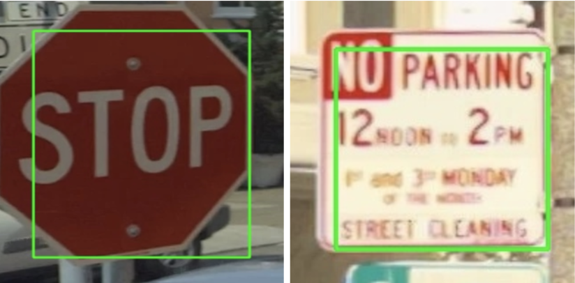
Figure 1.1: Sample sign detections from photos taken from cameras on vehicles.

One of the most challenging problems in building autonomous vehicles and route planning is constructing accurate maps. These maps are often algorithmically constructed from a combination of sources of information including satellite imagery, government data, street view imagery, and human labeling [26, 19]. These sources trade off cost and scalability with accuracy; as with most problems with big data, human labeling is accurate, but expensive. Therefore, improving the accuracy of automatic systems that can perform robust mapping in the presence of noisy detection and classification of objects would save both cost and effort.

$K$-means clustering is a common algorithm used for clustering data that come from different sources  [28, 5]. In the case of sensor fusion, the algorithm partitions data by assigning nearby objects to the nearest cluster using a metric such as Euclidean distance. There has been work in developing heuristic algorithms (e.g. Lloyd’s Algorithm [16]) for improving clustering in certain domains. For the problem of sensor fusion, it is often overconfident about false detections, as it fails to incorporate prior information and uncertainty about observation parameters such as observer location.

We propose a probabilistic model that performs bundle adjustment with road signs at scale, learning measurement parameters, e.g. observable radius and GPS error, while triangulating the probable locations of signs through an agglomerative clustering algorithm. This algorithm performs expectation maximization (EM) via message passing and Newton’s method. Critically, the clustering solver is differentiable, so its parameters can be learned jointly with stochastic variational inference (SVI). Optimization by inference requires a generative model, i.e. a model that describes how latent variables produce observed data. The generative model generates clusters given ray origins and directions given camera and neural net confidence parameters. It is used in conjunction with the clustering solver in a variational inference setting to optimize the global parameters.

We show that precision and recall can be increased with domain-specific priors and by incorporating data such as road networks. Since not every geographic region has both road network data and labeled ground truth, we learn maximum a posteriori (MAP) estimates of geographic parameters offline with limited data, which can be used to generalize to signs in different geographic regions.

Our contributions are as follows:

• We implement a differentiable soft clustering algorithm that uses loopy belief propagation (BP) to solve a data association problem and a differentiable Newton solver to predict cluster locations.

• We propose a generative model and an approximate inference model that is used to learn model parameters end-to-end on partially-labeled data.

• We learn parameters unique to each type of traffic object, and incorporate prior information in the form of road networks, learning e.g. where each type of traffic object is typically located w.r.t roads.

• We develop heuristics such as sparsification, eccentricity pruning, and locally sensitive hashing to scale to data batches of over 10,000 rays and 1000 objects on each compute node.

• We evaluate our method against SOTA methods used in production to build maps at scale.

2 Related work

Our system jointly performs object clustering, 3-D triangulation [8], and Bayesian training of parameters for sensor noise characteristics and object distributions.

Joint tracking and calibration has a long history, e.g. Lin et al  [15]. Using bearings-only sensors, Houssineau et al. [10] developed a unified approach to multi-object triangulation and parameter learning for sensor calibration. Ristic et al. [23] developed a joint algorithm for multi-target tracking and sensor bias estimation based on the Probability Hypothesis Density (PHD) filter.

The PHD filter [18] and labelled multi-Bernoulli filter [22] represent collections of unknown number of objects with unknown positions; our representation can be seen as a Laplace approximation to a multi-Bernoulli filter. To track multiple objects with unlabeled detections, Williams and Lau [27] solve the data association problem by using loopy belief propagation [20] to produce an approximate soft assignment of detections to objects. Turner et al. [25] describe a similar loopy BP-based multi-object tracking system, formulating the tracker as a variational inference method [3], similar to our formulation.

The recent availability of automatic differentiation frameworks like PyTorch [21] has led to more end-to-end learning approaches in localization [12] and tracking [11]. One crucial advance has been the ability to differentiate through solutions of optimization problems [6, 1] to enable nested optimization.

2.1 Variational inference

Probabilistic inference intends to infer distributions or values of latent variables $z$ given observed variables $x$ according to a probability distribution $p(z|x)=p(x,z)/p(x)$. Variational inference [3] is an approximate inference technique that treats probabilistic inference as an optimization problem by fitting an approximate distribution $q(z|x;\theta)$ to the model $p(x,z)$ by maximizing the evidence lower bound (ELBO)

$$\mathbf{ELBO}=\arg\max_{\theta}\mathbb{E}_{\bm{q}(z)}\bigl{[}\bm{p}(x,z)-\bm{q}(z|x;\theta)\bigr{]}$$ (2.1)

When variational parameters are shared across data, variational inference is amenable to stochastic optimization via minibatching (stochastic gradient variational Bayes [14]) and random sampling of latent variables (stochastic variational inference [9]).

Selecting an appropriate variational distribution is an open research problem and is often subject to the particulars of a given problem. A common variational family is the mean-field variational family, which imposes independence among the latent variables, i.e. the variational distribution factorizes completely:

$$q_{\text{mean\_field}}(z)=\prod_{i}q(z_{i})$$ (2.2)

Variational inference has recently become easier to scale to complex models through the use of automatic differentiation frameworks [21] and high level probabilistic programming languages [4, 2]. These tools can compute multiple derivatives through complex control flow, and leverage a number of techniques for variational inference including the reparameterization trick, Rao-Blackwellization, and automatic collapsing of discrete latent variables. For example, whereas previous optimization approaches have leveraged robust least squares solvers [17], AD frameworks permit regularized Newton solvers on symbolically computed likelihood functions, hence permitting a wider class of likelihoods and loss functions in models.

Probabilistic programming languages (PPLs) [4, 2] generalize probabilistic graphical models (PGMs) by allowing control flow, recursion, and other high level programming features in probabilistic models. A probabilistic program with static single assignments and no control flow corresponds to a probabilistic graphical model.

3 Method

3.1 Joint probabilistic data association

The data assignment of rays to clusters is solved with an EM algorithm, iteratively alternating between computing expectations of assignments and maximizing object locations at each step. Our EM algorithm consists of two phases: during the E-step, we use loopy belief propagation to compute the marginal association probabilities of assignments from detections (rays) to objects.

For each object $i\in\{1,...,n\}$ let $e_{i}\in\{0,1\}$ be the existence variable which is $1$ if the detection exists and $0$ otherwise. Similarly, let $a_{ij}\in\{0,1\}$ be the assignment variable which is $1$ if measurement $i$ is assigned to detection $j$ and $0$ otherwise. False detections are incorporated in $a_{ij}$ by assigning measurements to a ghost cluster if they associate with no detections. We can think about this setup as a bipartite graph with detections and clusters as nodes and assignments as edges. Then the joint probability of the existence and assignment logits is as follows:

$$P(e,a)\propto\gamma(e,a)\prod_{i}\psi_{i}^{e_{i}}\prod_{ij}\psi_{ij}^{a_{ij}}$$ (3.1)

where

$$\psi^{e_{i}}=\alpha_{i}\prod_{j}(1-p_{d}(x_{i},j))$$ (3.2)

$$\psi^{a_{ij}}=\delta_{i,j}\frac{f(z_{j}\mid x_{i})}{f_{\rm FD}(z_{j})}$$ (3.3)

$$\gamma(e,a)=\begin{cases}1,&\text{if $a_{i,j}\leq e_{i,j}\forall i,j$}.\\ 0,&\text{otherwise}.\end{cases}$$ (3.4)

and $\alpha_{i}$ is the existence logit, $\delta_{i,j}$ is the detection logit, and $f/f_{\rm FD}$ is the density ratio of the assignment logits.

The pairwise marginals for each edge in the graph can be approximated by loopy BP. We define $\mu_{ij}$ to be the message passed from $e_{i}\rightarrow a_{ij}$ and $\nu_{ij}$ to be the message passed in the reverse direction: $a_{ij}\rightarrow e_{i}$. The messages being passed are as follows:

$$\mu_{ij}=\frac{\psi_{i}\prod_{k\neq j}\nu_{kj}}{1+\psi_{i}\prod_{k\neq j}\nu_{kj}}$$ (3.5)

$$\nu_{ij}=1+\frac{\psi_{ij}}{1+\sum_{l\neq i}\psi_{lj}\mu_{lj}}$$ (3.6)

$$\overline{e_{i}}=\frac{\psi_{i}\prod_{j}\nu_{ij}}{1+\psi_{i}\prod_{j}\nu_{ij}}$$ (3.7)

$$\overline{a_{ij}}=\frac{\psi_{ij}\mu_{ij}}{1+\sum_{k}\psi_{kj}\mu_{kj}}$$ (3.8)

This algorithm converges quickly; in our experiments, we run the loopy BP algorithm for only 5 iterations. We then perform the M-step with a regularized Newton solver and update cluster locations and merge nearby clusters within a certain radius. Instead of a least squares solver, we use a twice differentiable log likelihood and directly apply a regularized Newton step as in equation (3.9). This also allows us to add in other log-likelihood terms such as a geographic prior.

$$\mathbf{x}_{n+1}=\mathbf{x}_{n}-[\mathbf{H}+\lambda\mathbf{I}]^{-1}\nabla f(\mathbf{x}_{n})\quad\forall\ n\geq 0.$$ (3.9)

${\bf H}$ is the Hessian and $\lambda$ is the regularization factor. The matrix solve is inexpensive because ${\bf H}$ has block diagonal structure with blocks of size only 2 or 3 (for 2D or 3D mapping, respectively); hence we can run this jointly over a tensor of thousands of clusters. The optimum found by the Newton solver is differentiable with respect to the solver inputs [6] so we can backpropagate through the solution to later learn global parameters.

Algorithm 1 EM Clustering

1:input $R$

2:$x\leftarrow\textrm{init}(R)$

3:while not converged do:

4:     // E-step:

5:     $p_{a},p_{ae}=\textrm{LoopyBP}(\log p_{d}(x,R))$

6:     // M-step:

7:     $loss=\sum_{i,j}p_{ae}(i,j)\log p_{d}(x_{i},R_{j})$

8:     $x_{n}\leftarrow\textrm{NewtonStep}(loss,x)$

9:     $x_{n}\leftarrow\textrm{merge(prune(}x_{n}))$

Algorithm 2 LoopyBP

1:input $p_{a}$

2:$\mu_{f},\mu_{b}=0$

3:while not converged do:

4:     $\mu_{f}\leftarrow\log(1-\exp(\mu_{f}-\rm{sum}(\mu_{b})-p_{a}))$

5:     $p_{ae}\leftarrow\exp(\mu_{f}+p_{a})$

6:     $\mu_{b}\leftarrow\log(1+\exp(p_{a}-\log(1+\exp(\rm{sum}(p_{ae})-p_{ae}))))$

7:return $p_{a},p_{e}$

Algorithm 3 NewtonStep

1:input $x,loss$

2:$g\leftarrow\mathbf{grad}(loss)$

3:$H\leftarrow\mathbf{grad}(g_{1}\ldots g_{n})$

4:$H_{\rm reg}\leftarrow H+g/r-\lambda_{\rm min}$

5:$x_{\rm new}\leftarrow x-H^{-1}_{\rm reg}g$

6:return $x_{\rm new}$

For our experiments, we take one Newton step after loopy BP has converged and we run Algorithm  1 for 10 iterations. Our implementations are open source .

3.2 Inference

Our sensor model incorporates two components: a radial component to model obstruction and invisibility of distant objects (modeled as an Exponential distribution); and an angular component to model a combination of orientation error of the sensor platform and segmentation error in the deep object detector. We do not attempt to estimate the true pose of each camera, since our partitioned data seldom leads to more than one detection per camera frame; this is in contrast to traditional bundle adjustment algorithms that can jointly estimate pose from multiple detections per image. We instead account for GPS error by approximately convolving our radial-angular likelihood by a Gaussian. To make this easier to compute, we preserve the Exponential radial component and model the angular component as a radius-dependent Von Mises distribution. The resulting 3-parameter distribution is shown in figure  3.1. During SVI training we learn all three parameters.

Figure 3.1: Observable distribution with GPS error and a radius of 50 meters.

To train with variational inference, we need to minimize the Kullback–Leibler (KL) divergence between the true posterior under our model prior and the variational distribution produced by the assignment solver. The ELBO we maximize (equivalent to minimizing the KL) can be written as:

$$\mathbf{ELBO}=\mathbb{E}_{r,\phi\sim q}[\log\bm{p}_{\theta}(e,a,x)-\log\bm{q}_{\theta}(e,a)]$$ (3.10)

where $\bm{q}$ is the distribution produced by the clustering solver parameterized by $\theta$, and $e$ and $a$ are existence and assignment variables respectively. In this training scheme, SVI is the outermost optimization algorithm, taking one gradient step per multiple iterations of the EM algorithm. Because of the Newton solver’s quadratic convergence rate, we can run without gradients (“detached”) in all but the final iteration, and propagate gradients back through only the final output of the loopy BP. This property is especially helpful because extra clusters at early iterations are often pruned or merged by the final iteration.

The assignment solver we use to produce the variational distribution generates soft assignments of the rays to clusters. These uncertainty estimates are useful when making predictions, especially in the context of building maps for autonomous vehicles. During training we make a mean-field approximation that each object’s assignment to rays is independent of other object’s assignments, so that the assignment distribution factors into independent Categorical distributions. This approximation allows us to exactly marginalize out assignments, leading to lower-variance gradient estimates than if we had used Monte Carlo sampling. This practice is common in soft-assignment EM algorithms.

We approximate the generative process of the clusters as a multi-Bernoulli process [22]. We experiment with two prior densities of objects: first a uniform density over the geographic region, and second a Spike-and-slab distribution discussed in section 4.7.

Since our data is largely unlabeled, we train in a semisupervised manner. Specifically, in areas with labeled ground truth, we probabilistically assign detections to known objects, assuming all objects are accounted for in ground truth. In areas without ground truth, we predict candidate clusters via Algorithm  1. Note that even though the ground truth is known in certain areas, it only provides the candidate clusters; the data association problem is still unsupervised.

3.3 Heuristics

The number of possible assignments grows quadratically with the number of clusters. To reduce cost, we employ an initialization scheme similar to probabilistic space carving, whereby we initialize candidate clusters along ray intersections. By rasterizing the image and initializing along regions with concentrated rays, we can reduce the computation time of the clustering algorithm.

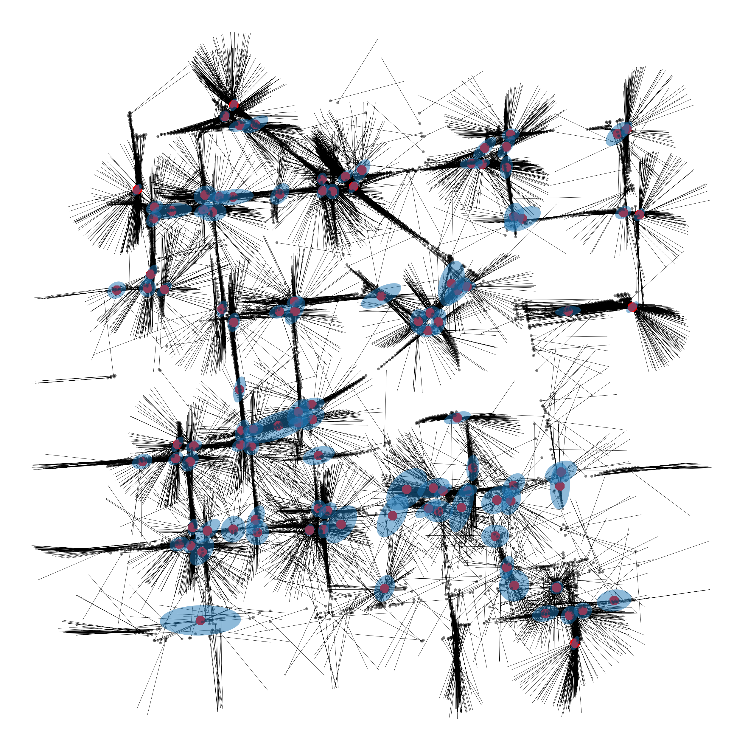
Figure 3.2: Ellipses of predicted clusters from the eccentricity of assigned rays.

To eliminate false detections that arise when two rays “look past each other” (i.e. lie on the same line in opposite directions), we compute the eccentricity of the detection from the eigenvalues of its assigned rays as shown in figure  3.2. We then prune clusters based on an eccentricity threshold. The intuition is that a true detection (especially one that is not eclipsed by buildings) will be observable from multiple angles. Naturally, this varies per sign type since the visibility of signs are subject to their location and surroundings. We do something similar with the covariance matrices of the clusters as well, thresholding them with a variance threshold.

Because the ray-cluster assignment problem is very sparse, we implement sparse tensor versions of the EM algorithm and BP algorithm, simultaneously assigning tens of thousands of rays to thousands of clusters on multi-CPU or GPU machines. This is critical for scaling up training on GPUs. We also implement locally sensitive hashing to efficiently merge nearby clusters greedily.

4 Experiments

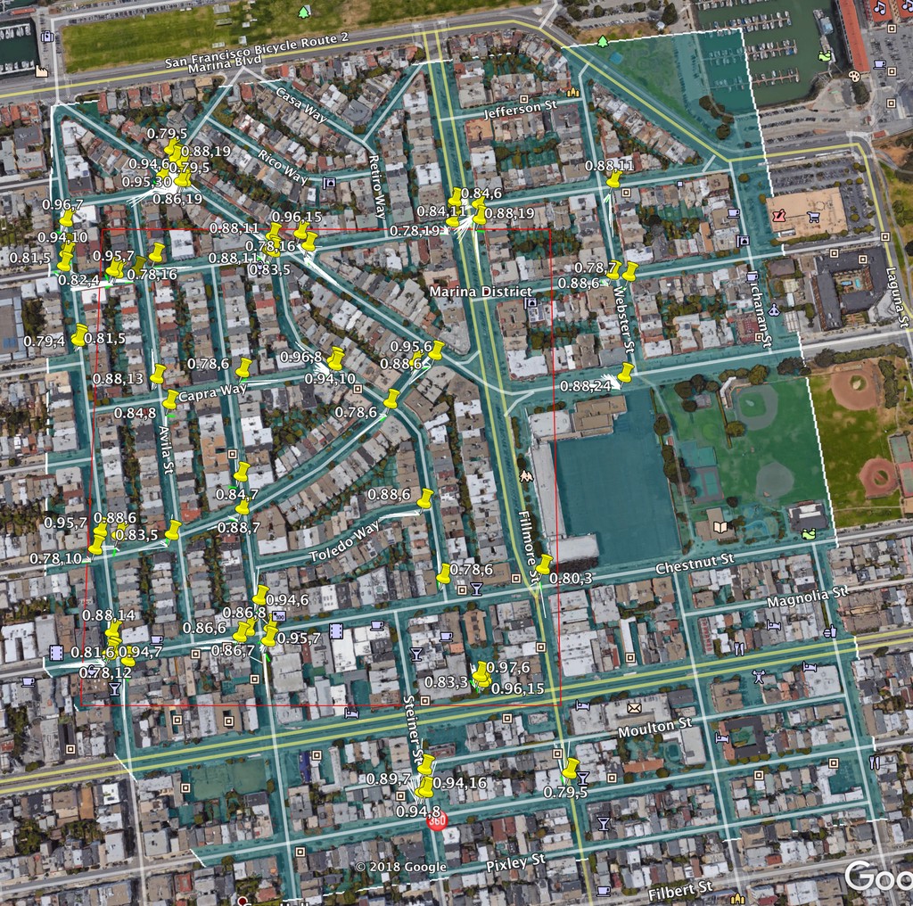
Figure 4.1: Predicted Stop sign locations (in yellow on the left and red on the right) for a 5x5 block region in San Francisco, CA. Note in the figure on the right that the ground truth labels (blue crosses) for Stop signs are incomplete in the region. The assignment solver has no knowledge of the ground truth clusters.

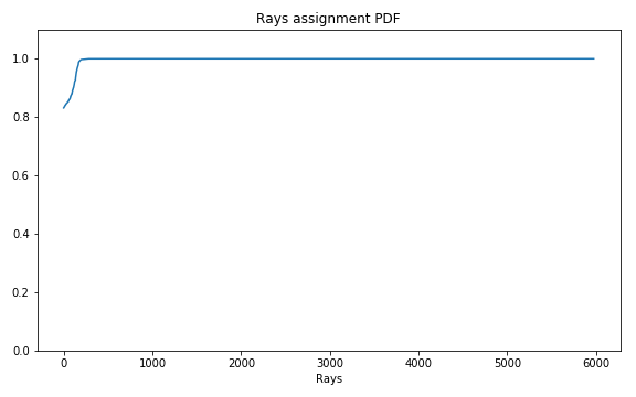
Figure 4.2: CDF of assignment probabilities of rays for Stop signs.

We run the clustering algorithm with both initial hand-tuned and trained parameters, and compare precision-recall and F1 metrics against the $K$-means clustering baseline. We consider each cluster within a 10 meter radius of a ground truth object as a true positive and additional clusters inside or outside the radius as false positives. We implement all algorithms in PyTorch [21] and Pyro [2].

4.1 Data

The main input data consists of rays denoted by the origin GPS position, the direction of the detection as a unit vector, and a confidence score from the DNN classifier. We focus primarily on Stop signs since they are the canonical case of sign detection and among the most critical for autonomous vehicles and ETA estimation. We look at three regions with ground truth in San Francisco: one four-way intersection, a 5x5 block area, and across a city (approximately ten 5x5 blocks of data). For Stop signs, a typical 5x5 block contains roughly 6000 rays and may contain anywhere from 60 to 100 Stop signs. We also look at other sign types in these regions with ground truth data since they have different detection accuracies, characteristics, and/or typical locations than Stop signs. This will allow us to measure how well SVI generalizes to different sign types.

4.2 Evaluation

We evaluate our models against the baseline by looking at three key metrics: precision, recall, and area under the curve (AUC), which is the integral of the precision-recall curve and our primary metric of interest. We look at two regions in particular: the 5x5 block and city level in San Francisco. The city data consists 10 non-contiguous 5x5 blocks. We threshold the output clusters below a certain probability before calculating metrics, using the same threshold across all three models.

4.3 SVI training

We train 8 parameters for every sign type concurrently; since sign-specific parameters are independent, the training scheme parallelizes easily. We train only in regions where we have some ground truth, though even then, ground truth coverage is only partial in these regions. Training is subject to the coverage and accuracy of the ground truth, since SVI will attempt to explain away rays within a truth region that are not associated with a true cluster. In areas where the true clusters are sparse e.g. Crosswalk signs, we notice that SVI training does not make improvements over the manual initialization scheme.

We incorporate pruning thresholds as non-trainable parameters during training but loosen them during prediction especially for signs with sparse numbers of rays (e.g. Pull through, Crosswalk signs) since these scenarios lack enough rays for eccentricity and variance to be a meaningful indicator of the quality of the detection.

Discrete latent variables such as the Categorical variables in the assignment distribution are known to produce high variance gradient estimates [24, 7]. To obtain lower-variance gradient estimates, we enumerate out discrete variables, performing exact inference for discrete latents in both our model and the variational approximation. This eliminates gradient estimator variance due to sampling latent variables, so that the only remaining source of variance during training is the random subsampling of data minibatches.

We train with the Adam optimizer [13] using a learning rate of 0.001 and anneal the learning rate with a decay factor of 0.7. We partition data into minibatches of approximately 5x5-block regions that contain anywhere from 40 to 7000 rays each. We run 5 iterations of loopy belief propagation and 10 EM iterations per SVI step.

SVI learns location-varying parameters such as GPS variance, which may be subject to the location of the vehicle. We assume GPS variance to be static and possibly slowly varying in space e.g. vary between residential and industrial areas of cities due to varying effects of occlusions due to buildings.

4.4 Quantitative results

Figure 4.3: Precision-recall plot for Stop signs in a 5x5 region. Note the improvement in AUC for the SVI-tuned model.

Figure 4.4: Predicted Stop sign locations (in yellow on the left and red on the right) for a 5x5 block region in San Francisco, CA. Note in the figure on the right that the ground truth labels (blue crosses) for Stop signs are incomplete in the region. The assignment solver has no knowledge of the ground truth clusters.

		Stop	Crosswalk	DoNotEnter	NoLeft	LeftYield	NoRight	NoRightCond	NoLeftU	2WayTraffic
	Truth	228	56	54	50	2	19	4	6	11
baseline	Prec	0.68	0.5	0.6	0.52	0.5	1.0	0.0	0.0	1.0
	Recall	0.87	0.55	0.63	0.6	0.5	0.26	0.0	0.0	0.18
	AUC	0.74	0.44	0.55	0.44	0.57	0.26	0.0	0.0	0.18
manual	Prec	0.82	0.74	0.88	0.7	1.0	0.91	0.2	0.62	0.67
	Recall	0.84	0.41	0.52	0.52	0.5	0.53	0.25	0.83	0.36
	AUC	0.83	0.46	0.64	0.46	0.81	0.55	0.03	0.77	0.32
SVI	Prec	0.84	0.76	0.88	0.72	1.0	0.91	0.5	0.62	0.67
	Recall	0.83	0.45	0.52	0.52	0.5	0.53	0.5	0.83	0.36
	AUC	0.85	0.46	0.63	0.48	0.81	0.55	0.31	0.77	0.32

Table 1: Results on road signs for the city region in San Francisco. AUC = Area under the curve, which is our primary metric of interest. The baseline is the $k$-means clustering algorithm. “Manual” is the EM algorithm with hand tuned parameters. “SVI” is the EM algorithm with parameters tuned by SVI. Note that the ground truth is incomplete so precision numbers should be higher for all three methods.

		Stop	Crosswalk	Yield	StateRoute	TempParking	Merge	DoNotEnter
Without priors	Prec	0.4	0.60	0.55	0.12	0.14	0.43	0.63
	Recall	0.88	0.52	0.79	1.0	0.53	1.0	0.85
With priors	Prec	0.42	0.63	0.61	0.14	0.17	0.50	0.71
	Recall	0.88	0.52	0.79	1.0	0.53	1.0	0.85

Table 2: Results on road signs with and without a road network in various regions in Austin, TX. Regions are all approximately 4x4 blocks and were selected based on regions where there was the highest density of ground truth.

We evaluate our algorithm on the precision/recall curve evaluated over an entire city, the largest region. During training, the algorithm only trains in the ground truth regions and for Stop signs, only in one 5x5 region, which means that the other 9 5x5 blocks are not viewed during training. At test time, the models predict on all the regions together. The results are shown in table  1.

There are a few important trends to note here. The first is that our algorithm outperforms the baseline in most circumstances with either parameter setting. In instances where the baseline performs better, especially in recall, the difference is often by an order of magnitude less than the difference in which our algorithm outperforms the baseline. The next trend to note is that SVI tends to produce equal or better results than the initial hand tuned parameters. This gives us reasonable confidence that for sign types that have enough ground truth for a trainable signal, the algorithm will learn parameters that are consistent with real world observations. This is further reaffirmed by the fact that for sign types that have very few ground truth and detections such as Left Yield or No Left U-turn, SVI learns parameters that do not differ significantly from the initialization.

The metric of particular interest is the AUC, which measures the precision-recall trade-off of these algorithms make. For all but one sign type, SVI has the best AUC; in one exception it is 0.01 below the hand-tuned model. While the baseline has relatively high recall, especially with sign types that are abundant in the region, it has lower precision and AUC than our Bayesian algorithm.

In summary, we find that SVI successfully learns global parameter values even in the presence of unknown data associations and limited ground truth data. More importantly, it allows a single hierarchical generative model to generalize to different sign types by learning parameters for each sign type. As long as we are reasonably confident that our generative model is faithful to real world observations, we can reuse the same model to train a variety of clustering solvers for different traffic objects.

4.5 Confidence Tuning

We learn the confidence scores of the rays as a sign-specific parameter. The upstream neural detector often gives an unreliable confidence score, and so we learn confidence parameters correlating the detector issued confidence and its probability of associating with a cluster. In figure 4.2, observe that most of the rays for Stop signs are pretty reliable; the algorithm was able to assign over 5000 rays to clusters, though this is not the case for say Crosswalk signs.

4.6 False detections

False detections take the form of objects similarly colored or shaped as real signs. These objects exist as detections but are fewer in number than true detections since an object that appears to be a sign in one frame could be correctly classified as not a sign in later frames as the camera approaches the object. This naturally affects rarer signs more than common signs since there are not enough rays for the algorithm to be confident it is a false detection. For signs such as Stop signs, the ratio true detections to false detections is higher than that of Crosswalk signs, which have much fewer detections.

Without eccentricity and variance pruning, the curve is fairly consistent since all the remaining clusters are of high confidence since presumably more detections contributed to that cluster. Without the pruning, recall dramatically increases at the cost of precision since clusters in the middle streets arise from two observations that see sign behind the other. Without thresholding, a sparse number of detections would lead to the presence of low probability clusters.

4.7 Intersection parameter training

We incorporate further prior information in cities where we have access to the road network as an ablation study. We train a MAP estimate of the intersection affinity for each sign type. This training can be done completely offline (i.e. outside of the SVI training loop), as it is fitting parameters directly to a road network, and as such, does not require the EM solver or the generative model used in SVI.

We use a Spike-and-slab prior over the entire area which places a Gaussian distribution at intersections and Uniform distribution everywhere else as in figure  4.4. We train on a road network in Austin, TX, and compare clustering prediction results between those with a prior over the road network and those without (i.e. a Uniform prior across the entire region). We learn the affinity of signs to intersections given an intersection radius, which is the scale of the Gaussian. These parameters can theoretically also be transferred across cities since traffic laws are almost identical across states which means signs are used in the same capacity (e.g. Stop signs are located at intersections and require a complete stop for all cities in the US).

We test in different regions per sign type since the ground truth is sparse across the city, with each region roughly consisting of 12-25 contiguous blocks in a rectangle. We manually select regions with a high concentration of ground truth and run both models identically with the exception of the additional prior. As displayed Table  2, the streetmap prior seems to not affect the recall, as both models perform identically for all sign types. It seems to help on precision, giving strictly better results than the version without. One explanation for this is that we use a sparse prior which is most effective in culling out outlier clusters. A true cluster usually has many detections associated with it, which makes it likely for the clustering algorithm to predict a sign there, regardless of the streetmap prior i.e. the prior provides weak information. A false detection however, often comes from a few sporadic rays that don’t necessarily converge at a single point. In the presence of the streetmap prior we use, it can possibly be dropped, depending on how close the candidate location is to an intersection and the sign’s affinity to be near intersections.

5 Conclusion

We present a framework for sensor fusion through stochastic optimization. We introduce an end-to-end trainable EM clustering algorithm that solves the JPDA problem, which is trained with a generative model through variational inference. We demonstrate an improvement in results through a combination of heuristics and additional prior information. This technique can be used for problems that employ bundle adjustment, and has real world impact in the development of mapping technology.

We would like to eventually train the upstream DNN detector, in an active learning setup, where the predicted clusters from our clustering algorithm could be used as ground truth for the classifier. In this setup, both the detector and the clustering algorithm can be trained in a completely unsupervised manner.

6 Acknowledgments

We would like to thank Martin Jankowiak, Peter Dayan, Karl Obermeyer for helpful discussions and advice, Felipe Such for help running experiments, and the Pyro team for software support.

References

- [1] B. Amos and J. Z. Kolter. Optnet: Differentiable optimization as a layer in neural networks. arXiv preprint arXiv:1703.00443, 2017.
- [2] E. Bingham, J. P. Chen, M. Jankowiak, F. Obermeyer, N. Pradhan, T. Karaletsos, R. Singh, P. Szerlip, P. Horsfall, and N. D. Goodman. Pyro: Deep Universal Probabilistic Programming. arXiv preprint arXiv:1810.09538, 2018.
- [3] D. M. Blei, A. Kucukelbir, and J. D. McAuliffe. Variational inference: A review for statisticians. Journal of the American Statistical Association, 112(518):859–877, 2017.
- [4] B. Carpenter, A. Gelman, M. D. Hoffman, D. Lee, B. Goodrich, M. Betancourt, M. Brubaker, J. Guo, P. Li, and A. Riddell. Stan: A probabilistic programming language. Journal of statistical software, 76(1), 2017.
- [5] M. Gönen and A. A. Margolin. Localized data fusion for kernel k-means clustering with application to cancer biology. In Advances in Neural Information Processing Systems, pages 1305–1313, 2014.
- [6] S. Gould, B. Fernando, A. Cherian, P. Anderson, R. S. Cruz, and E. Guo. On differentiating parameterized argmin and argmax problems with application to bi-level optimization. arXiv preprint arXiv:1607.05447, 2016.
- [7] W. Grathwohl, D. Choi, Y. Wu, G. Roeder, and D. Duvenaud. Backpropagation through the void: Optimizing control variates for black-box gradient estimation. arXiv preprint arXiv:1711.00123, 2017.
- [8] R. I. Hartley and P. Sturm. Triangulation. Computer vision and image understanding, 68(2):146–157, 1997.
- [9] M. D. Hoffman, D. M. Blei, C. Wang, and J. Paisley. Stochastic variational inference. The Journal of Machine Learning Research, 14(1):1303–1347, 2013.
- [10] J. Houssineau, D. E. Clark, S. Ivekovic, C. S. Lee, and J. Franco. A unified approach for multi-object triangulation, tracking and camera calibration. IEEE Transactions on Signal Processing, 64(11):2934–2948, 2016.
- [11] R. Jonschkowski, D. Rastogi, and O. Brock. Differentiable particle filters: End-to-end learning with algorithmic priors. arXiv preprint arXiv:1805.11122, 2018.
- [12] P. Karkus, D. Hsu, and W. S. Lee. Particle filter networks: End-to-end probabilistic localization from visual observations. arXiv preprint arXiv:1805.08975, 2018.
- [13] D. P. Kingma and J. Ba. Adam: A method for stochastic optimization. arXiv preprint arXiv:1412.6980, 2014.
- [14] D. P. Kingma and M. Welling. Auto-encoding variational bayes. arXiv preprint arXiv:1312.6114, 2013.
- [15] X. Lin, Y. Bar-Shalom, and T. Kirubarajan. Exact multisensor dynamic bias estimation with local tracks. IEEE transactions on Aerospace and Electronic Systems, 40(2):576–590, 2004.
- [16] S. Lloyd. Least squares quantization in pcm. IEEE transactions on information theory, 28(2):129–137, 1982.
- [17] M. Lourakis and A. Argyros. The design and implementation of a generic sparse bundle adjustment software package based on the levenberg-marquardt algorithm. Technical report, Technical Report 340, Institute of Computer Science-FORTH, Heraklion, Crete, Greece, 2004.
- [18] R. Mahler. Phd filters of higher order in target number. IEEE Transactions on Aerospace and Electronic systems, 43(4), 2007.
- [19] G. Máttyus, S. Wang, S. Fidler, and R. Urtasun. Hd maps: Fine-grained road segmentation by parsing ground and aerial images. In Proceedings of the IEEE Conference on Computer Vision and Pattern Recognition, pages 3611–3619, 2016.
- [20] K. P. Murphy, Y. Weiss, and M. I. Jordan. Loopy belief propagation for approximate inference: An empirical study. In Proceedings of the Fifteenth conference on Uncertainty in artificial intelligence, pages 467–475. Morgan Kaufmann Publishers Inc., 1999.
- [21] A. Paszke, S. Gross, S. Chintala, G. Chanan, E. Yang, Z. DeVito, Z. Lin, A. Desmaison, L. Antiga, and A. Lerer. Automatic differentiation in pytorch. In NIPS-W, 2017.
- [22] S. Reuter, B.-T. Vo, B.-N. Vo, and K. Dietmayer. The labeled multi-bernoulli filter. IEEE Trans. Signal Processing, 62(12):3246–3260, 2014.
- [23] B. Ristic, D. E. Clark, and N. Gordon. Calibration of multi-target tracking algorithms using non-cooperative targets. IEEE Journal of Selected Topics in Signal Processing, 7(3):390–398, 2013.
- [24] G. Tucker, A. Mnih, C. J. Maddison, J. Lawson, and J. Sohl-Dickstein. Rebar: Low-variance, unbiased gradient estimates for discrete latent variable models. In Advances in Neural Information Processing Systems, pages 2627–2636, 2017.
- [25] R. D. Turner, S. Bottone, and B. Avasarala. A complete variational tracker. In Advances in Neural Information Processing Systems, pages 496–504, 2014.
- [26] J. D. Wegner, S. Branson, D. Hall, K. Schindler, and P. Perona. Cataloging public objects using aerial and street-level images-urban trees. In Proceedings of the IEEE Conference on Computer Vision and Pattern Recognition, pages 6014–6023, 2016.
- [27] J. Williams and R. Lau. Approximate evaluation of marginal association probabilities with belief propagation. IEEE Transactions on Aerospace and Electronic Systems, 50(4):2942–2959, 2014.
- [28] S. Yu, L. Tranchevent, X. Liu, W. Glanzel, J. A. Suykens, B. De Moor, and Y. Moreau. Optimized data fusion for kernel k-means clustering. IEEE Transactions on Pattern Analysis and Machine Intelligence, 34(5):1031–1039, 2012.