Coupled Multirate Infinitesimal GARK Schemes for Stiff Systems with Multiple Time Scales

Abstract

Traditional time discretization methods use a single timestep for the entire system of interest and can perform poorly when the dynamics of the system exhibits a wide range of time scales. Multirate infinitesimal step (MIS) methods (Knoth and Wolke, 1998) offer an elegant and flexible approach to efficiently integrate such systems. The slow components are discretized by a Runge–Kutta method, and the fast components are resolved by solving modified fast differential equations. Sandu (2018) developed the Multirate Infinitesimal General-structure Additive Runge–Kutta (MRI-GARK) family of methods that includes traditional MIS schemes as a subset. The MRI-GARK framework allowed the construction of the first fourth order MIS schemes. This framework also enabled the introduction of implicit methods, which are decoupled in the sense that any implicitness lies entirely within the fast or slow integrations. It was shown by Sandu that the stability of decoupled implicit MRI-GARK methods has limitations when both the fast and slow components are stiff and interact strongly. This work extends the MRI-GARK framework by introducing coupled implicit methods to solve stiff multiscale systems. The coupled approach has the potential to considerably improve the overall stability of the scheme, at the price of requiring implicit stage calculations over the entire system. Two coupling strategies are considered. The first computes coupled Runge–Kutta stages before solving a single differential equation to refine the fast solution. The second alternates between computing coupled Runge–Kutta stages and solving fast differential equations. We derive order conditions and perform the stability analysis for both strategies. The new coupled methods offer improved stability compared to the decoupled MRI-GARK schemes. The theoretical properties of the new methods are validated with numerical experiments.

65L05, 65L06

1 Introduction

In this paper, we consider the additively partitioned ordinary differential equation (ODE)

(1) $$y^{\prime}=f(t,y)=f^{\left\{\mathfrak{f}\right\}}(t,y)+f^{\left\{\mathfrak{s}\right\}}(t,y),\qquad y(t_{0})=y_{0}\in\mathbbm{R}^{d},$$

where component $f^{\left\{\mathfrak{f}\right\}}$ represents the fast dynamics of the system, and component $f^{\left\{\mathfrak{s}\right\}}$ the slow dynamics. This structure models a feature appearing in many dynamical systems of practical interest: multiple characteristic time scales.

Multirate time integration methods are designed to efficiently solve Eq. 1 by using different timesteps for the fast and slow components. First explored by Rice [28] and Andrus [2, 3], the multirating strategy has been expanded to numerous types of traditional time integration methods. This includes Runge–Kutta methods [7, 13, 14, 23, 24, 33, 29], linear multistep methods [11, 18, 31], Rosenbrock-W methods [12], extrapolation methods [8, 10], Galerkin discretizations [25], and combined multiscale methodologies [9].

Multirate infinitesimal step (MIS) methods, first proposed by Knoth and Wolke [22], and later extended by others [21, 36, 37, 38, 40], introduce a new multirating philosophy in which the fast method solves a modified ODE that advances the solution between slow stages. While the slow system is solved discretely, the fast system can be solved with arbitrary small steps, hence the naming “infinitesimal step”. In [15], Günther and Sandu cast MIS methods into the General-structure Additive Runge–Kutta (GARK) framework. This framework was subsequently leveraged by Sandu in [30] to create the multirate infinitesimal GARK (MRI-GARK) class of methods. One step of an MRI-GARK method advances the solution from $t_{n}$ to $t_{n}+H$ by

(2a) $$Y_{1}=y_{n}$$

(2b) $$\left\{\begin{aligned} v_{i}(0)&=Y_{i},\\ T_{i}&=t_{n}+\mathbase{c}^{\left\{\mathfrak{s}\right\}}_{i}\,H,\\ v_{i}^{\prime}&={\Delta\mathbase{c}}^{\left\{\mathfrak{s}\right\}}_{i}\,f^{\left\{\mathfrak{f}\right\}}\left(T_{i}+{\Delta\mathbase{c}}^{\left\{\mathfrak{s}\right\}}_{i}\,\theta,v_{i}\right)+\sum_{j=1}^{i+1}\gamma_{i,j}\left(\tfrac{\theta}{H}\right)\,f^{\left\{\mathfrak{s}\right\}}\left(T_{j},Y_{j}\right),\\ &\quad\text{for }\theta\in[0,H],\\ Y_{i+1}&=v_{i}(H),\qquad i=1,\dots,s^{\left\{\mathfrak{s}\right\}},\end{aligned}\right.$$

(2c) $$y_{n+1}=Y_{s^{\left\{\mathfrak{s}\right\}}+1},$$

where $\mathbase{c}^{\left\{\mathfrak{s}\right\}}$ are the slow method abscissae, and the modified fast ODEs $v_{i}^{\prime}=\dots$ advance the solution between the slow stages. In [30], Sandu presents MRI-GARK methods Eq. 2 of orders up to four that are explicit or implicit in the fast and slow systems but are not coupled across partitions. This work also provides new techniques in investigating the stability of partitioned methods that we have adopted in our paper. Recent developments in the field include the work of Sexton and Reynolds [39] where a new structure for fast integration weights is considered and shown to help reduce order conditions; the “relaxed MIS” methods derived retain the same order as traditional MIS and it is possible to pair them for error control and adaptivity purposes.

This work extends the MRI-GARK family [30] to include implicit methods with coupling between slow and fast systems. We construct two new families of schemes designed to offer improved stability compared to decoupled MRI-GARK methods. The first family is step predictor-corrector MRI-GARK methods that perform a coupled discrete prediction over the entire timestep, then use that information to perform an infinitesimal step correction with small timesteps. This is similar to the strategy used by Rice in [28] and Savcenco in [34, 35]. The second family is internal stage predictor-corrector MRI-GARK methods that alternate between coupled discrete predictor stages and infinitesimal step correction ones. Figure 1 shows the differences between the new strategies and previous approaches. Order condition theories and stability analyses are developed for both new families of methods, and schemes up to order four are designed. Numerical experiments are employed to verify the theoretical findings.

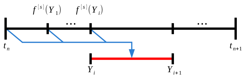
(a) Traditional multirate infinitesimal schemes use previously computed stages, which means the slow tendencies are extrapolated in the formulation of modified fast systems.

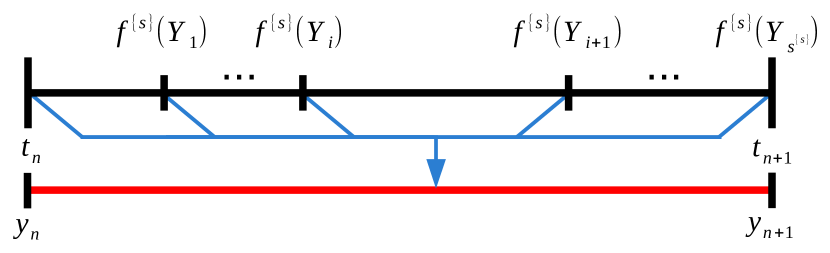
(b) The newly proposed step predictor-corrector MRI-GARK schemes use all stages for computing slow tendencies and solve a single fast ODE over the entire step.

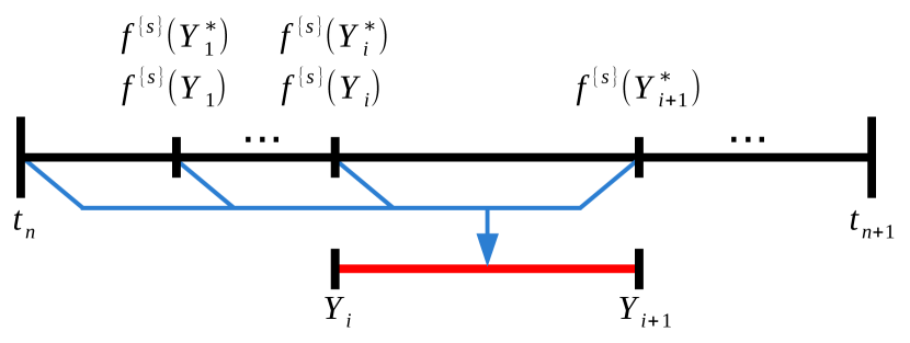
(c) The newly proposed internal stage predictor-corrector MRI-GARK schemes use previously computed stages and a predicted next stage, which allows for interpolation of slow tendencies in the formulation of modified fast systems.

Figure 1: Comparison of MRI-GARK schemes: blue arrows indicate stage dependencies of the modified fast ODE and the red lines indicate the intervals over which a fast ODE is solved.

The paper is organized as follows. The new family of step predictor corrector MRI-GARK schemes is introduced in Section 2, followed by its order condition theory and the stability analysis. In Section 3, internal stage predictor corrector MRI-GARK schemes are defined and their order conditions and stability are established. Numerical results are reported in Section 4, and concluding remarks are drawn in Section 5. Appendix A presents the lists of coefficients and stability plots for the newly developed methods.

2 Step predictor-corrector MRI-GARK methods

One coupling strategy commonly used in discrete multirate methods is a predictor-corrector approach, where the predictor evolves the entire system, while the corrector is only applied to the fast partition whose solution was “predicted” inaccurately (see [28, 34, 35]). First, a combined Runge–Kutta macro-step is taken which serves as the predictor. The fast parts of the predicted stages are inaccurate and are refined by sub-stepping the fast component only. Approximations of the slow values needed during the micro-steps are obtained from interpolating the slow predicted values. The step predictor-corrector MRI-GARK methods, as depicted in Fig. 1(b), can be viewed as an extreme case of this coupling strategy where the multirate ratio is infinite, i.e., the corrector takes infinitely many steps to refine the fast solution.

2.1 Method definition

We start with a “slow” Runge–Kutta base method

(3) $$\begin{array}[]{c|c}\mathbase{c}^{\left\{\mathfrak{s}\right\}}&\mathbase{A}^{\left\{\mathfrak{s},\mathfrak{s}\right\}}\\ \hline\cr&\mathbase{b}^{\left\{\mathfrak{s}\right\}T}\\ \hline\cr&\widehat{\mathbase{b}}^{\left\{\mathfrak{s}\right\}T}\end{array}$$

with $s^{\left\{\mathfrak{s}\right\}}$ stages. Unlike other multirate infinitesimal strategies, the base method is not restricted to be explicit or diagonally implicit.

Definition 2.1 (Step predictor corrector MRI-GARK methods).

One step of a step predictor-corrector MRI-GARK (SPC-MRI-GARK) scheme applied to Eq. 1 is given by

(4a) $$Y_{i}=y_{n}+H\sum_{j=1}^{s^{\left\{\mathfrak{s}\right\}}}\,\mathbase{a}^{\left\{\mathfrak{s}\right\}}_{i,j}f_{j},\quad i=1,\dots,s^{\left\{\mathfrak{s}\right\}},$$

(4b) $$\left\{\begin{aligned} v(0)&=y_{n},\\ v^{\prime}&=f^{\left\{\mathfrak{f}\right\}}(t_{n}+\theta,v)+\sum_{j=1}^{s^{\left\{\mathfrak{s}\right\}}}\gamma_{j}\left(\tfrac{\theta}{H}\right)\,f^{\left\{\mathfrak{s}\right\}}_{j},\quad\text{for }\theta\in[0,H],\\ y_{n+1}&=v(H),\end{aligned}\right.$$

where $f_{j}\coloneqq f\big{(}t_{n}+\mathbase{c}^{\left\{\mathfrak{s}\right\}}_{j}\,H,Y_{j}\big{)}$ and $f_{j}^{\left\{\mathfrak{s}\right\}}\coloneqq f^{\left\{\mathfrak{s}\right\}}\big{(}t_{n}+\mathbase{c}^{\left\{\mathfrak{s}\right\}}_{j}\,H,Y_{j}\big{)}$.

Definition 2.2 (Slow tendency coefficients [30, Definition 2.2]).

The time-dependent coefficients in Eq. 4b are defined as polynomials:

(5) $$\gamma_{i}(t)\coloneqq\sum_{k\geq 0}\gamma_{i}^{k}\,t^{k},\quad\widetilde{\gamma}_{i}(t)\coloneqq\int_{0}^{t}\gamma_{i}(\tau)\,\differential\tau=\sum_{k\geq 0}\gamma_{i}^{k}\frac{t^{k+1}}{k+1},\quad\overline{\gamma}_{i}\coloneqq\widetilde{\gamma}_{i}(1).$$

Remark 2.3 (Embedded method).

An embedded solution for an SPC-MRI-GARK method can be computed by solving the additional ODE

$$\left\{\begin{aligned} \widehat{v}(0)&=y_{n},\\ \widehat{v}^{\prime}&=f^{\left\{\mathfrak{f}\right\}}\left(t_{n}+\theta,\widehat{v}\right)+\sum_{j=1}^{s^{\left\{\mathfrak{s}\right\}}}\widehat{\gamma}_{j}\left(\tfrac{\theta}{H}\right)\,f^{\left\{\mathfrak{s}\right\}}_{j},\quad\text{for }\theta\in[0,H],\\ \widehat{y}_{n+1}&=\widehat{v}(H),\end{aligned}\right.$$

which uses the embedded polynomials $\widehat{\gamma}_{i}$ and produces a solution of a different order. We note that although this additional integration can be expensive, it can be done in parallel with Eq. 4b.

Consider the trivial partitioning $f^{\left\{\mathfrak{f}\right\}}=0$, $f^{\left\{\mathfrak{s}\right\}}=f$ of Eq. 1. In this case, it is natural to expect an SPC-MRI-GARK method to degenerate into the slow base method. Note that the final solution of Eq. 4b simplifies to

(6) $$y_{n+1}=y_{n}+\int_{0}^{H}\sum_{j=1}^{s^{\left\{\mathfrak{s}\right\}}}\gamma_{j}\left(\tfrac{\theta}{H}\right)\,f^{\left\{\mathfrak{s}\right\}}_{j}\differential{\theta}=y_{n}+H\sum_{j=1}^{s^{\left\{\mathfrak{s}\right\}}}\overline{\gamma}_{j}\,f_{j}^{\left\{\mathfrak{s}\right\}}.$$

Thus, we enforce the condition

(7) $$\mathbase{b}^{\left\{\mathfrak{s}\right\}}=\overline{\gamma}.$$

An important special case of (1) are component partitioned systems:

(8) $$\begin{bmatrix}y^{\left\{\mathfrak{f}\right\}}\\ y^{\left\{\mathfrak{s}\right\}}\end{bmatrix}^{\prime}=\begin{bmatrix}f^{\left\{\mathfrak{f}\right\}}\left(t,y^{\left\{\mathfrak{f}\right\}},y^{\left\{\mathfrak{s}\right\}}\right)\\ f^{\left\{\mathfrak{s}\right\}}\left(t,y^{\left\{\mathfrak{f}\right\}},y^{\left\{\mathfrak{s}\right\}}\right)\end{bmatrix}=\begin{bmatrix}f^{\left\{\mathfrak{f}\right\}}\left(t,y^{\left\{\mathfrak{f}\right\}},y^{\left\{\mathfrak{s}\right\}}\right)\\ 0\end{bmatrix}+\begin{bmatrix}0\\ f^{\left\{\mathfrak{s}\right\}}\left(t,y^{\left\{\mathfrak{f}\right\}},y^{\left\{\mathfrak{s}\right\}}\right)\end{bmatrix}.$$

One step of an SPC-MRI-GARK method Eq. 4 applied to Eq. 8 reads:

(9a) $$\begin{bmatrix}Y^{\left\{\mathfrak{f}\right\}}_{i}\\ Y^{\left\{\mathfrak{s}\right\}}_{i}\end{bmatrix}=\begin{bmatrix}y^{\left\{\mathfrak{f}\right\}}_{n}+H\sum_{j=1}^{s^{\left\{\mathfrak{s}\right\}}}\mathbase{a}^{\left\{\mathfrak{s}\right\}}_{i,j}\,f^{\left\{\mathfrak{f}\right\}}_{j}\\ y^{\left\{\mathfrak{s}\right\}}_{n}+H\sum_{j=1}^{s^{\left\{\mathfrak{s}\right\}}}\mathbase{a}^{\left\{\mathfrak{s}\right\}}_{i,j}\,f^{\left\{\mathfrak{s}\right\}}_{j}\end{bmatrix},$$

(9b) $$\left\{\begin{aligned} v^{\left\{\mathfrak{f}\right\}}(0)&=y^{\left\{\mathfrak{f}\right\}}_{n},\\ {v^{\left\{\mathfrak{f}\right\}}}^{\prime}&=f^{\left\{\mathfrak{f}\right\}}\left(t_{n}+\theta,v,y^{\left\{\mathfrak{s}\right\}}_{n}+H\sum_{j=1}^{s^{\left\{\mathfrak{s}\right\}}}\widetilde{\gamma}_{j}\left(\tfrac{\theta}{H}\right)\,f_{j}^{\left\{\mathfrak{s}\right\}}\right),\quad\text{for }\theta\in[0,H]\\ \begin{bmatrix}y^{\left\{\mathfrak{f}\right\}}_{n+1}\\ y^{\left\{\mathfrak{s}\right\}}_{n+1}\end{bmatrix}&=\begin{bmatrix}v^{\left\{\mathfrak{f}\right\}}(H)\\ y^{\left\{\mathfrak{s}\right\}}_{n}+H\sum_{j=1}^{s^{\left\{\mathfrak{s}\right\}}}\mathbase{b}^{\left\{\mathfrak{s}\right\}}_{j}\,f^{\left\{\mathfrak{s}\right\}}_{j}\end{bmatrix},\end{aligned}\right.$$

where $f^{\left\{\mathfrak{f}\right\}}_{j}\coloneqq f^{\left\{\mathfrak{f}\right\}}\big{(}t_{n}+\mathbase{c}^{\left\{\mathfrak{s}\right\}}_{j}\,H,Y^{\left\{\mathfrak{f}\right\}}_{j},Y^{\left\{\mathfrak{s}\right\}}_{j}\big{)}$ and $f^{\left\{\mathfrak{s}\right\}}_{j}\coloneqq f^{\left\{\mathfrak{s}\right\}}\big{(}t_{n}+\mathbase{c}^{\left\{\mathfrak{s}\right\}}_{j}\,H,Y^{\left\{\mathfrak{f}\right\}}_{j},Y^{\left\{\mathfrak{s}\right\}}_{j}\big{)}$. With Eqs. 6 and 7 the internal ODE integrates (and corrects) only the fast component, while the slow component is solved with the traditional base Runge–Kutta method (3).

2.2 Order conditions

Following [30], we use an arbitrarily accurate Runge–Kutta method $\left(A^{\left\{\mathfrak{f},\mathfrak{f}\right\}},b^{\left\{\mathfrak{f}\right\}},c^{\left\{\mathfrak{f}\right\}}\right)$ to discretize the continuous ODE appearing in the method formulation, which casts the SPC-MRI-GARK scheme (4) into the GARK framework. The discrete corrector stages, denoted $Y^{\left\{\mathfrak{f},\right\}}_{i}$, are computed as

$$Y^{\left\{\mathfrak{f},\right\}}_{i} =y_{n}+H\sum_{j=1}^{s^{\left\{\mathfrak{f}\right\}}}a^{\left\{\mathfrak{f},\mathfrak{f}\right\}}_{i,j}\left(f^{\left\{\mathfrak{f},\right\}}_{j}+\sum_{\ell=1}^{s^{\left\{\mathfrak{s}\right\}}}\gamma_{\ell}\big{(}c^{\left\{\mathfrak{f}\right\}}_{j}\big{)}\,f^{\left\{\mathfrak{s}\right\}}_{\ell}\right),$$

$$=y_{n}+H\sum_{j=1}^{s^{\left\{\mathfrak{f}\right\}}}a^{\left\{\mathfrak{f},\mathfrak{f}\right\}}_{i,j}\,f^{\left\{\mathfrak{f},\right\}}_{j}+H\sum_{\ell=1}^{s^{\left\{\mathfrak{s}\right\}}}\left(\sum_{j=1}^{s^{\left\{\mathfrak{f}\right\}}}a^{\left\{\mathfrak{f},\mathfrak{f}\right\}}_{i,j}\,\gamma_{\ell}\big{(}c^{\left\{\mathfrak{f}\right\}}_{j}\big{)}\right)f^{\left\{\mathfrak{s}\right\}}_{\ell},$$

$$=y_{n}+H\sum_{j=1}^{s^{\left\{\mathfrak{f}\right\}}}a^{\left\{\mathfrak{f},\mathfrak{f}\right\}}_{i,j}\,f^{\left\{\mathfrak{f},\right\}}_{j}+H\sum_{j=1}^{s^{\left\{\mathfrak{s}\right\}}}\left(\sum_{k\geq 0}A^{\left\{\mathfrak{f},\mathfrak{f}\right\}}\,c^{\left\{\mathfrak{f}\right\}\times k}\,{\gamma^{k}}^{T}\right)_{i,j}f^{\left\{\mathfrak{s}\right\}}_{j},$$

where $f^{\left\{\mathfrak{f},\right\}}_{j}\coloneqq f^{\left\{\mathfrak{f}\right\}}\big{(}t_{n}+c^{\left\{\mathfrak{f}\right\}}_{j}\,H,Y^{\left\{\mathfrak{f},\right\}}_{j}\big{)}$ and the superscript $\times k$ denotes the elementwise vector power. Similarly, the final solution reads

$$y_{n+1} =y_{n}+H\sum_{j=1}^{s^{\left\{\mathfrak{f}\right\}}}b^{\left\{\mathfrak{f}\right\}}_{j}\,f^{\left\{\mathfrak{f},\right\}}_{j}+H\sum_{j=1}^{s^{\left\{\mathfrak{s}\right\}}}\left(\sum_{k\geq 0}b^{\left\{\mathfrak{f}\right\}T}\,c^{\left\{\mathfrak{f}\right\}\times k}\right)f^{\left\{\mathfrak{s}\right\}}_{j},$$

$$=y_{n}+H\sum_{j=1}^{s^{\left\{\mathfrak{f}\right\}}}b^{\left\{\mathfrak{f}\right\}}_{j}\,f^{\left\{\mathfrak{f},\right\}}_{j}+H\sum_{j=1}^{s^{\left\{\mathfrak{s}\right\}}}\left(\sum_{k\geq 0}\frac{1}{k+1}\gamma_{j}^{k}\right)f^{\left\{\mathfrak{s}\right\}}_{j},$$

$$=y_{n}+H\sum_{j=1}^{s^{\left\{\mathfrak{f}\right\}}}b^{\left\{\mathfrak{f}\right\}}_{j}f^{\left\{\mathfrak{f},\right\}}_{j}+H\sum_{j=1}^{s^{\left\{\mathfrak{s}\right\}}}\overline{\gamma}_{j}\,f^{\left\{\mathfrak{s}\right\}}_{j},$$

$$=y_{n}+H\sum_{j=1}^{s^{\left\{\mathfrak{f}\right\}}}b^{\left\{\mathfrak{f}\right\}}_{j}\,f^{\left\{\mathfrak{f},\right\}}_{j}+H\sum_{j=1}^{s^{\left\{\mathfrak{s}\right\}}}\mathbase{b}^{\left\{\mathfrak{s}\right\}}_{j}f^{\left\{\mathfrak{s}\right\}}_{j}.$$

Now, the corresponding GARK tableau for an SPC-MRI-GARK method is

$$\begin{array}[]{c|cc|c|c}\mathbase{c}^{\left\{\mathfrak{s}\right\}}&\mathbase{A}^{\left\{\mathfrak{s},\mathfrak{s}\right\}}&0&\mathbase{A}^{\left\{\mathfrak{s},\mathfrak{s}\right\}}&\mathbase{c}^{\left\{\mathfrak{s}\right\}}\\ c^{\left\{\mathfrak{f}\right\}}&0&A^{\left\{\mathfrak{f},\mathfrak{f}\right\}}&\sum_{k\geq 0}A^{\left\{\mathfrak{f},\mathfrak{f}\right\}}\,c^{\left\{\mathfrak{f}\right\}\times k}\,{\gamma^{k}}^{T}&c^{\left\{\mathfrak{f},\mathfrak{s}\right\}}\\ \hline\cr\mathbase{c}^{\left\{\mathfrak{s}\right\}}&\mathbase{A}^{\left\{\mathfrak{s},\mathfrak{s}\right\}}&0&\mathbase{A}^{\left\{\mathfrak{s},\mathfrak{s}\right\}}&\mathbase{c}^{\left\{\mathfrak{s}\right\}}\\ \hline\cr&0&b^{\left\{\mathfrak{f}\right\}T}&\mathbase{b}^{\left\{\mathfrak{s}\right\}T}\end{array},$$

with $c^{\left\{\mathfrak{f},\mathfrak{s}\right\}}=\sum_{k\geq 0}A^{\left\{\mathfrak{f},\mathfrak{f}\right\}}\,c^{\left\{\mathfrak{f}\right\}\times k}\,{\gamma^{k}}^{T}\,\mathbbm{1}^{\left\{\mathfrak{s}\right\}}$.

2.2.1 Internal consistency

Theorem 2.4 (Internal consistency conditions).

An SPC-MRI-GARK method Eq. 4 satisfies the “internal consistency” conditions

$$\mathbf{c}^{\left\{\mathfrak{s},\mathfrak{f}\right\}}=\mathbf{c}\SS\equiv\mathbase{c}^{\left\{\mathfrak{s}\right\}}\quad\text{and}\quad\mathbf{c}^{\left\{\mathfrak{f},\mathfrak{f}\right\}}=\mathbf{c}^{\left\{\mathfrak{f},\mathfrak{s}\right\}}$$

for any fast method iff the following conditions hold:

(10) $${\gamma^{0}}^{T}\,\mathbbm{1}^{\left\{\mathfrak{s}\right\}}=1\quad\text{and}\quad{\gamma^{k}}^{T}\,\mathbbm{1}^{\left\{\mathfrak{s}\right\}}=0\quad\forall k\geq 1.$$

Proof 2.5.

All internal consistency equations are automatically satisfied except for the following one, which needs to be imposed explicitly:

$$c^{\left\{\mathfrak{f}\right\}} =\sum_{k\geq 0}A^{\left\{\mathfrak{f},\mathfrak{f}\right\}}\,c^{\left\{\mathfrak{f}\right\}\times k}\,{\gamma^{k}}^{T}\,\mathbbm{1}^{\left\{\mathfrak{s}\right\}}.$$

It is easy to confirm Eq. 10 is sufficient to satisfy this condition, and thus, internal consistency. Since the equality must hold for all $A^{\left\{\mathfrak{f},\mathfrak{f}\right\}}$, it must hold when all $A^{\left\{\mathfrak{f},\mathfrak{f}\right\}}\,c^{\left\{\mathfrak{f}\right\}\times k}$ are linearly independent. Matching powers of the left- and right-hand sides proves the necessity of Eq. 10.

If an SPC-MRI-GARK method has a slow base method Eq. 3 of order two, then internal consistency is sufficient to guarantee the method is order two [32].

2.2.2 Fourth order conditions

In this section, we derive order conditions of the SPC-MRI-GARK schemes for up to order four. First, we define a set of useful coefficients.

Definition 2.6 (Some useful coefficients [30, Definition 3.3]).

Consider the “bushy” Butcher tree [16]

(11) $$\mathfrak{t}_{k}\coloneqq[\underbrace{\tau,\dots,\tau}_{k\text{ times}}]\in T,$$

where $\tau\in T$ is the tree of order one and $[\cdot]$ is the operation of joining subtrees by a root. An arbitrarily accurate Runge–Kutta method $\left(A^{\left\{\mathfrak{f},\mathfrak{f}\right\}},b^{\left\{\mathfrak{f}\right\}},c^{\left\{\mathfrak{f}\right\}}\right)$ satisfies the following equations:

(12) $$\zeta_{k} \coloneqq\frac{1}{\gamma\left([\mathfrak{t}_{k}]\right)} =b^{\left\{\mathfrak{f}\right\}T}\,A^{\left\{\mathfrak{f},\mathfrak{f}\right\}}\,c^{\left\{\mathfrak{f}\right\}\times k} =\frac{1}{(k+1)(k+2)},$$

$$\omega_{k} \coloneqq\frac{1}{\gamma\left([\tau,\mathfrak{t}_{k}]\right)} =\left(b^{\left\{\mathfrak{f}\right\}}\times c^{\left\{\mathfrak{f}\right\}}\right)^{T}A^{\left\{\mathfrak{f},\mathfrak{f}\right\}}\,c^{\left\{\mathfrak{f}\right\}\times k} =\frac{1}{(k+1)(k+3)},$$

$$\xi_{k} \coloneqq\frac{1}{\gamma\left([[\mathfrak{t}_{k}]]\right)} =b^{\left\{\mathfrak{f}\right\}T}\,A^{\left\{\mathfrak{f},\mathfrak{f}\right\}}\,A^{\left\{\mathfrak{f},\mathfrak{f}\right\}}\,c^{\left\{\mathfrak{f}\right\}\times k} =\frac{1}{(k+1)(k+2)(k+3)}.$$

Theorem 2.7 (Fourth order coupling conditions).

An internally consistent SPC-MRI-GARK method Eq. 4 satisfying Eq. 7 has order four iff the slow base scheme Eq. 3 has order at least four, and the following coupling conditions hold:

(13a) $$\frac{1}{6} =\sum_{k\geq 0}\zeta_{k}\,{\gamma^{k}}^{T}\,\mathbase{c}^{\left\{\mathfrak{s}\right\}},$$ (order 3)

(13b) $$\frac{1}{8} =\sum_{k\geq 0}\omega_{k}\,{\gamma^{k}}^{T}\,\mathbase{c}^{\left\{\mathfrak{s}\right\}},$$ (order 4)

(13c) $$\frac{1}{12} =\sum_{k\geq 0}\zeta_{k}\,{\gamma^{k}}^{T}\,\mathbase{c}^{\left\{\mathfrak{s}\right\}\times 2},$$ (order 4)

(13d) $$\frac{1}{24} =\sum_{k\geq 0}\zeta_{k}\,{\gamma^{k}}^{T}\,\mathbase{A}^{\left\{\mathfrak{s},\mathfrak{s}\right\}}\,\mathbase{c}^{\left\{\mathfrak{s}\right\}}.$$ (order 4)

Proof 2.8.

An internally consistent GARK scheme is order four iff the base methods are order four and the 12 coupling conditions up to order four are satisfied [32]. We proceed with checking each coupling condition.

Condition 3a

The first third order condition gives Eq. 13a:

$$\frac{1}{6}=\mathbf{b}^{\left\{\mathfrak{f}\right\}T}\,\mathbf{A}^{\left\{\mathfrak{f},\mathfrak{s}\right\}}\,\mathbf{c}^{\left\{\mathfrak{s}\right\}}=\sum_{k\geq 0}\zeta_{k}\,{\gamma^{k}}^{T}\,\mathbase{c}^{\left\{\mathfrak{s}\right\}}.$$

Condition 3b

The other third order condition is automatically satisfied if the slow base method is order three:

$$\frac{1}{6}=\mathbf{b}^{\left\{\mathfrak{s}\right\}T}\,\mathbf{A}^{\left\{\mathfrak{s},\mathfrak{f}\right\}}\,\mathbf{c}^{\left\{\mathfrak{f}\right\}}=\mathbase{b}^{\left\{\mathfrak{s}\right\}T}\,\mathbase{A}^{\left\{\mathfrak{s},\mathfrak{s}\right\}}\,\mathbase{c}^{\left\{\mathfrak{s}\right\}}.$$

Condition 4a

The first fourth order condition gives Eq. 13b:

$$\frac{1}{8}=\left(\mathbf{b}^{\left\{\mathfrak{f}\right\}}\times\mathbf{c}^{\left\{\mathfrak{f}\right\}}\right)^{T}\mathbf{A}^{\left\{\mathfrak{f},\mathfrak{s}\right\}}\,\mathbf{c}^{\left\{\mathfrak{s}\right\}}=\sum_{k\geq 0}\omega_{k}\,{\gamma^{k}}^{T}\,\mathbase{c}^{\left\{\mathfrak{s}\right\}}.$$

Condition 4b

This condition is automatically satisfied if the slow base method is order four:

$$\frac{1}{8}=\left(\mathbf{b}^{\left\{\mathfrak{s}\right\}}\times\mathbf{c}^{\left\{\mathfrak{s}\right\}}\right)^{T}\mathbf{A}^{\left\{\mathfrak{s},\mathfrak{f}\right\}}\,\mathbf{c}^{\left\{\mathfrak{f}\right\}}=\left(\mathbase{b}^{\left\{\mathfrak{s}\right\}}\times\mathbase{c}^{\left\{\mathfrak{s}\right\}}\right)^{T}\mathbase{A}^{\left\{\mathfrak{s},\mathfrak{s}\right\}}\,\mathbase{c}^{\left\{\mathfrak{s}\right\}}.$$

Condition 4c

This condition proves Eq. 13c:

$$\frac{1}{12}=\mathbf{b}^{\left\{\mathfrak{f}\right\}T}\,\mathbf{A}^{\left\{\mathfrak{f},\mathfrak{s}\right\}}\,\mathbf{c}^{\left\{\mathfrak{s}\right\}\times 2}=\sum_{k\geq 0}\zeta_{k}\,{\gamma^{k}}^{T}\,\mathbase{c}^{\left\{\mathfrak{s}\right\}\times 2}.$$

Condition 4d

This condition is automatically satisfied if the slow base method is order four:

$$\frac{1}{12}=\mathbf{b}^{\left\{\mathfrak{s}\right\}T}\,\mathbf{A}^{\left\{\mathfrak{s},\mathfrak{f}\right\}}\,\mathbf{c}^{\left\{\mathfrak{f}\right\}\times 2}=\mathbase{b}^{\left\{\mathfrak{s}\right\}T}\,\mathbase{A}^{\left\{\mathfrak{s},\mathfrak{s}\right\}}\,\mathbase{c}^{\left\{\mathfrak{s}\right\}\times 2}.$$

Condition 4e

This condition is the redundant since it is the difference of Condition 3a and 4a:

$$\frac{1}{24}=\mathbf{b}^{\left\{\mathfrak{f}\right\}T}\,\mathbf{A}^{\left\{\mathfrak{f},\mathfrak{f}\right\}}\,\mathbf{A}^{\left\{\mathfrak{f},\mathfrak{s}\right\}}\,\mathbf{c}^{\left\{\mathfrak{s}\right\}}=\sum_{k\geq 0}\xi_{k}\,{\gamma^{k}}^{T}\,\mathbase{c}^{\left\{\mathfrak{s}\right\}}.$$

Condition 4f

This condition proves Eq. 13d:

$$\frac{1}{24}=\mathbf{b}^{\left\{\mathfrak{f}\right\}T}\,\mathbf{A}^{\left\{\mathfrak{f},\mathfrak{s}\right\}}\,\mathbf{A}^{\left\{\mathfrak{s},\mathfrak{f}\right\}}\,\mathbf{c}^{\left\{\mathfrak{f}\right\}}=\sum_{k\geq 0}\zeta_{k}\,{\gamma^{k}}^{T}\,\mathbase{A}^{\left\{\mathfrak{s},\mathfrak{s}\right\}}\,\mathbase{c}^{\left\{\mathfrak{s}\right\}}.$$

Condition 4g

The following condition is identical to Condition 4f:

$$\frac{1}{24}=\mathbf{b}^{\left\{\mathfrak{f}\right\}T}\,\mathbf{A}^{\left\{\mathfrak{f},\mathfrak{s}\right\}}\,\mathbf{A}\SS\,\mathbf{c}^{\left\{\mathfrak{s}\right\}}=\sum_{k\geq 0}\zeta_{k}\,{\gamma^{k}}^{T}\,\mathbase{A}^{\left\{\mathfrak{s},\mathfrak{s}\right\}}\,\mathbase{c}^{\left\{\mathfrak{s}\right\}}.$$

Condition 4h

This condition is automatically satisfied if the slow base method is order four:

$$\frac{1}{24}=\mathbf{b}^{\left\{\mathfrak{s}\right\}T}\,\mathbf{A}\SS\,\mathbf{A}^{\left\{\mathfrak{s},\mathfrak{f}\right\}}\,\mathbf{c}^{\left\{\mathfrak{f}\right\}}=\mathbase{b}^{\left\{\mathfrak{s}\right\}T}\,\mathbase{A}^{\left\{\mathfrak{s},\mathfrak{s}\right\}}\,\mathbase{A}^{\left\{\mathfrak{s},\mathfrak{s}\right\}}\,\mathbase{c}^{\left\{\mathfrak{s}\right\}}.$$

Condition 4i

This condition is automatically satisfied if the slow base method is order four:

$$\frac{1}{24}=\mathbf{b}^{\left\{\mathfrak{s}\right\}T}\,\mathbf{A}^{\left\{\mathfrak{s},\mathfrak{f}\right\}}\,\mathbf{A}^{\left\{\mathfrak{f},\mathfrak{s}\right\}}\,\mathbf{c}^{\left\{\mathfrak{s}\right\}}=\mathbase{b}^{\left\{\mathfrak{s}\right\}T}\,\mathbase{A}^{\left\{\mathfrak{s},\mathfrak{s}\right\}}\,\mathbase{A}^{\left\{\mathfrak{s},\mathfrak{s}\right\}}\,\mathbase{c}^{\left\{\mathfrak{s}\right\}}.$$

Condition 4j

This condition is automatically satisfied if the slow base method is order four:

$$\frac{1}{24}=\mathbf{b}^{\left\{\mathfrak{s}\right\}T}\,\mathbf{A}^{\left\{\mathfrak{s},\mathfrak{f}\right\}}\,\mathbf{A}^{\left\{\mathfrak{f},\mathfrak{f}\right\}}\,\mathbf{c}^{\left\{\mathfrak{f}\right\}}=\mathbase{b}^{\left\{\mathfrak{s}\right\}T}\,\mathbase{A}^{\left\{\mathfrak{s},\mathfrak{s}\right\}}\,\mathbase{A}^{\left\{\mathfrak{s},\mathfrak{s}\right\}}\,\mathbase{c}^{\left\{\mathfrak{s}\right\}}.$$

Remark 2.9.

In the proof of Theorem 2.7, all coupling order conditions that start with $\mathbf{b}^{\left\{\mathfrak{s}\right\}T}$ collapse onto the order conditions of the slow base method. In the context of two-trees [4, 32], trees containing both slow and fast nodes with a slow root can be recolored into purely slow trees. The purely fast trees are of no concern since the fast base method is arbitrarily accurate. The remaining trees contain slow and fast nodes with a fast root, which correspond to coupling conditions Eq. 13 that must be explicitly enforced through the choice of $\gamma$.

2.3 Stability analysis

2.3.1 Scalar stability analysis

Consider the partitioned, linear, scalar test problem

(14) $$y^{\prime}=\lambda^{\left\{\mathfrak{f}\right\}}\,y+\lambda^{\left\{\mathfrak{s}\right\}}\,y,\qquad\lambda^{\left\{\mathfrak{f}\right\}},\lambda^{\left\{\mathfrak{s}\right\}}\in\mathbb{C}^{-},$$

and let $z^{\left\{\mathfrak{f}\right\}}\coloneqq H\,\lambda^{\left\{\mathfrak{f}\right\}}$, $z^{\left\{\mathfrak{s}\right\}}\coloneqq H\,\lambda^{\left\{\mathfrak{s}\right\}}$, and $z\coloneqq z^{\left\{\mathfrak{f}\right\}}+z^{\left\{\mathfrak{s}\right\}}$. Applying the SPC-MRI-GARK method (4) to Eq. 14 yields

$$Y=\left(I_{s^{\left\{\mathfrak{s}\right\}}\times s^{\left\{\mathfrak{s}\right\}}}-z\,\mathbase{A}^{\left\{\mathfrak{s},\mathfrak{s}\right\}}\right)^{-1}\mathbbm{1}^{\left\{\mathfrak{s}\right\}}y_{n},$$

$$\left\{\begin{aligned} v(0)&=y_{n},\\ v^{\prime}&=\lambda^{\left\{\mathfrak{f}\right\}}\,v+\lambda^{\left\{\mathfrak{s}\right\}}\sum_{j=1}^{s^{\left\{\mathfrak{s}\right\}}}\gamma_{j}\left(\tfrac{\theta}{H}\right)\,Y_{j},\\ &=\lambda^{\left\{\mathfrak{f}\right\}}\,v+\lambda^{\left\{\mathfrak{s}\right\}}\sum_{k\geq 0}\left(\tfrac{\theta}{H}\right)^{k}{\gamma^{k}}^{T}\,Y,\\ y_{n+1}&=\varphi_{0}\big{(}z^{\left\{\mathfrak{f}\right\}}\big{)}\,y_{n}+z^{\left\{\mathfrak{s}\right\}}\,\mu\big{(}z^{\left\{\mathfrak{f}\right\}}\big{)}^{T}\,Y,\end{aligned}\right.$$

which leads to the stability function

(15) $$\begin{split}y_{n+1}&=R\big{(}z^{\left\{\mathfrak{f}\right\}},z^{\left\{\mathfrak{s}\right\}}\big{)}\,y_{n},\\ R\big{(}z^{\left\{\mathfrak{f}\right\}},z^{\left\{\mathfrak{s}\right\}}\big{)}&\coloneqq\varphi_{0}\big{(}z^{\left\{\mathfrak{f}\right\}}\big{)}+z^{\left\{\mathfrak{s}\right\}}\,\mu\big{(}z^{\left\{\mathfrak{f}\right\}}\big{)}^{T}\left(I_{s^{\left\{\mathfrak{s}\right\}}\times s^{\left\{\mathfrak{s}\right\}}}-z\,\mathbase{A}^{\left\{\mathfrak{s},\mathfrak{s}\right\}}\right)^{-1}\mathbbm{1}^{\left\{\mathfrak{s}\right\}},\end{split}$$

where, following [30]:

$$\begin{split}\mu\big{(}z^{\left\{\mathfrak{f}\right\}}\big{)}&\coloneqq\sum_{k\geq 0}\gamma^{k}\,\varphi_{k+1}\big{(}z^{\left\{\mathfrak{f}\right\}}\big{)},\\ \varphi_{0}(z)&\coloneqq e^{z},\qquad\varphi_{k+1}(z)\coloneqq\int_{0}^{1}e^{z(1-t)}t^{k}\differential{t}=\begin{cases}\frac{e^{z}-1}{z}&k=0\\ \frac{k\varphi_{k}(z)-1}{z}&k>0\end{cases}.\end{split}$$

Of special interest are cases when a partition becomes infinitely stiff. If the base method has bounded internal stability, the stability function Eq. 15 enjoys the following property:

(16a) $$\lim_{z^{\left\{\mathfrak{f}\right\}}\to-\infty}R\big{(}z^{\left\{\mathfrak{f}\right\}},z^{\left\{\mathfrak{s}\right\}}\big{)}=0.$$

Provided $$\mathbase{A}^{\left\{\mathfrak{s},\mathfrak{s}\right\}}$$ is invertible, e.g. the base method is SDIRK,

(16b) $$\lim_{z^{\left\{\mathfrak{s}\right\}}\to-\infty}R\big{(}z^{\left\{\mathfrak{f}\right\}},z^{\left\{\mathfrak{s}\right\}}\big{)}=\varphi_{0}\big{(}z^{\left\{\mathfrak{f}\right\}}\big{)}-\mu\big{(}z^{\left\{\mathfrak{f}\right\}}\big{)}^{T}\left(\mathbase{A}^{\left\{\mathfrak{s},\mathfrak{s}\right\}}\right)^{-1}\mathbbm{1}^{\left\{\mathfrak{s}\right\}}.$$

Although Eq. 16b cannot be zero for all $z^{\left\{\mathfrak{f}\right\}}$ due to the linear independence of $\varphi$ functions, its modulus is bounded for $z^{\left\{\mathfrak{f}\right\}}\in\mathbb{C}^{-}$.

2.3.2 Matrix stability analysis

Following [23, 30], consider the matrix test problem

(17) $$\begin{bmatrix}y^{\left\{\mathfrak{f}\right\}}\\ y^{\left\{\mathfrak{s}\right\}}\end{bmatrix}^{\prime}=\begin{bmatrix}\lambda^{\left\{\mathfrak{f}\right\}}&\eta^{\left\{\mathfrak{s}\right\}}\\ \eta^{\left\{\mathfrak{f}\right\}}&\lambda^{\left\{\mathfrak{s}\right\}}\end{bmatrix}\begin{bmatrix}y^{\left\{\mathfrak{f}\right\}}\\ y^{\left\{\mathfrak{s}\right\}}\end{bmatrix}=\underbrace{\begin{bmatrix}\lambda^{\left\{\mathfrak{f}\right\}}&\frac{1-\xi}{\alpha}\left(\lambda^{\left\{\mathfrak{f}\right\}}-\lambda^{\left\{\mathfrak{s}\right\}}\right)\\ -\alpha\,\xi\left(\lambda^{\left\{\mathfrak{f}\right\}}-\lambda^{\left\{\mathfrak{s}\right\}}\right)&\lambda^{\left\{\mathfrak{s}\right\}}\end{bmatrix}}_{\boldsymbol{\Omega}}\begin{bmatrix}y^{\left\{\mathfrak{f}\right\}}\\ y^{\left\{\mathfrak{s}\right\}}\end{bmatrix}.$$

The change of variables that produces $\boldsymbol{\Omega}$ [30]

$$\alpha\coloneqq\frac{\lambda^{\left\{\mathfrak{f}\right\}}-\lambda^{\left\{\mathfrak{s}\right\}}+\delta}{2\,\eta^{\left\{\mathfrak{s}\right\}}missing},\quad\xi\coloneqq\frac{\lambda^{\left\{\mathfrak{f}\right\}}-\lambda^{\left\{\mathfrak{s}\right\}}-\delta}{2\left(\lambda^{\left\{\mathfrak{f}\right\}}-\lambda^{\left\{\mathfrak{s}\right\}}\right)},\quad\delta=\sqrt{4\,\eta^{\left\{\mathfrak{f}\right\}}\,\eta^{\left\{\mathfrak{s}\right\}}+\left(\lambda^{\left\{\mathfrak{f}\right\}}-\lambda^{\left\{\mathfrak{s}\right\}}\right)^{2}},$$

allows the matrix eigenvalues to be written as linear combinations of the diagonal entries: $\xi\,\lambda^{\left\{\mathfrak{f}\right\}}+(1-\xi)\,\lambda^{\left\{\mathfrak{s}\right\}}$ and $(1-\xi)\,\lambda^{\left\{\mathfrak{f}\right\}}+\xi\,\lambda^{\left\{\mathfrak{s}\right\}}$. The coupling between the fast and slow variables is controlled by $\xi$. Values close to zero indicate the slow system is weakly influenced by the fast one, while values close to one indicate the fast system is weakly influenced by the slow one.

Let

$$Z\coloneqq\begin{bmatrix}z^{\left\{\mathfrak{f}\right\}}&w^{\left\{\mathfrak{s}\right\}}\\ w^{\left\{\mathfrak{f}\right\}}&z^{\left\{\mathfrak{s}\right\}}\end{bmatrix}\coloneqq H\begin{bmatrix}\lambda^{\left\{\mathfrak{f}\right\}}&\eta^{\left\{\mathfrak{s}\right\}}\\ \eta^{\left\{\mathfrak{f}\right\}}&\lambda^{\left\{\mathfrak{s}\right\}}\end{bmatrix},\qquad\widetilde{\mu}\big{(}z^{\left\{\mathfrak{f}\right\}}\big{)}\coloneqq\sum_{k\geq 0}\frac{\gamma^{k}}{k+1}\varphi_{k+2}\big{(}z^{\left\{\mathfrak{f}\right\}}\big{)}.$$

The component partitioned SPC-MRI-GARK method Eq. 9 applied to the matrix test problem Eq. 17 gives

$$\begin{bmatrix}Y^{\left\{\mathfrak{f}\right\}}\\ Y^{\left\{\mathfrak{s}\right\}}\end{bmatrix}=\left(I_{2s^{\left\{\mathfrak{s}\right\}}\times 2s^{\left\{\mathfrak{s}\right\}}}-Z\otimes\mathbase{A}^{\left\{\mathfrak{s},\mathfrak{s}\right\}}\right)^{-1}\begin{bmatrix}y^{\left\{\mathfrak{f}\right\}}_{n}\,\mathbbm{1}^{\left\{\mathfrak{s}\right\}}\\ y^{\left\{\mathfrak{s}\right\}}_{n}\,\mathbbm{1}^{\left\{\mathfrak{s}\right\}}\end{bmatrix},$$

$$\left\{\begin{aligned} v^{\left\{\mathfrak{f}\right\}}(0)&=y^{\left\{\mathfrak{f}\right\}}_{n},\\ {v^{\left\{\mathfrak{f}\right\}}}^{\prime}&=\lambda^{\left\{\mathfrak{f}\right\}}\,v^{\left\{\mathfrak{f}\right\}}+\eta^{\left\{\mathfrak{s}\right\}}\,y^{\left\{\mathfrak{s}\right\}}_{n}+\eta^{\left\{\mathfrak{s}\right\}}\sum_{j=1}^{s^{\left\{\mathfrak{s}\right\}}}\widetilde{\gamma}_{j}\left(\tfrac{\theta}{H}\right)\left(w^{\left\{\mathfrak{f}\right\}}\,Y^{\left\{\mathfrak{f}\right\}}_{j}+z^{\left\{\mathfrak{s}\right\}}\,Y^{\left\{\mathfrak{s}\right\}}_{j}\right),\\ &=\lambda^{\left\{\mathfrak{f}\right\}}\,v^{\left\{\mathfrak{f}\right\}}+\eta^{\left\{\mathfrak{s}\right\}}\,y^{\left\{\mathfrak{s}\right\}}+\eta^{\left\{\mathfrak{s}\right\}}\sum_{k\geq 0}\frac{(\theta/H)^{k+1}}{k+1}{\gamma^{k}}^{T}\left(w^{\left\{\mathfrak{f}\right\}}\,Y^{\left\{\mathfrak{f}\right\}}+z^{\left\{\mathfrak{s}\right\}}\,Y^{\left\{\mathfrak{s}\right\}}\right),\\ \begin{bmatrix}y_{n+1}^{\left\{\mathfrak{f}\right\}}\\ y_{n+1}^{\left\{\mathfrak{s}\right\}}\end{bmatrix}&=\begin{bmatrix}v^{\left\{\mathfrak{f}\right\}}(H)\\ y^{\left\{\mathfrak{s}\right\}}_{n}+w^{\left\{\mathfrak{f}\right\}}\,\mathbase{b}^{\left\{\mathfrak{s}\right\}T}\,Y^{\left\{\mathfrak{f}\right\}}+z^{\left\{\mathfrak{s}\right\}}\,\mathbase{b}^{\left\{\mathfrak{s}\right\}T}\,Y^{\left\{\mathfrak{s}\right\}}\end{bmatrix},\end{aligned}\right.$$

We write the solution of the ODE as

$$y^{\left\{\mathfrak{f}\right\}}_{n+1}=\varphi_{0}\big{(}z^{\left\{\mathfrak{f}\right\}}\big{)}\,y^{\left\{\mathfrak{f}\right\}}_{n}+w^{\left\{\mathfrak{s}\right\}}\,\varphi_{1}\big{(}z^{\left\{\mathfrak{f}\right\}}\big{)}\,y^{\left\{\mathfrak{s}\right\}}_{n}+w^{\left\{\mathfrak{s}\right\}}\,\widetilde{\mu}\big{(}z^{\left\{\mathfrak{f}\right\}}\big{)}^{T}\left(w^{\left\{\mathfrak{f}\right\}}\,Y^{\left\{\mathfrak{f}\right\}}+z^{\left\{\mathfrak{s}\right\}}\,Y^{\left\{\mathfrak{s}\right\}}\right).$$

The transfer matrix for the matrix test problem can be written as

(18) $$\begin{split}\begin{bmatrix}y^{\left\{\mathfrak{f}\right\}}_{n+1}\\ y^{\left\{\mathfrak{s}\right\}}_{n+1}\end{bmatrix}&=\mathbf{M}\big{(}z^{\left\{\mathfrak{f}\right\}},z^{\left\{\mathfrak{s}\right\}},w^{\left\{\mathfrak{s}\right\}},w^{\left\{\mathfrak{f}\right\}}\big{)}\begin{bmatrix}y^{\left\{\mathfrak{f}\right\}}_{n}\\ y^{\left\{\mathfrak{s}\right\}}_{n}\end{bmatrix},\\ \mathbf{M}\big{(}z^{\left\{\mathfrak{f}\right\}},z^{\left\{\mathfrak{s}\right\}},w^{\left\{\mathfrak{s}\right\}},w^{\left\{\mathfrak{f}\right\}}\big{)}&\coloneqq\begin{bmatrix}\varphi_{0}(z^{\left\{\mathfrak{f}\right\}})&w^{\left\{\mathfrak{s}\right\}}\varphi_{1}\left(z^{\left\{\mathfrak{f}\right\}}\right)\\ 0&1\end{bmatrix}\\ &\quad+\begin{bmatrix}w^{\left\{\mathfrak{s}\right\}}\,w^{\left\{\mathfrak{f}\right\}}\,\widetilde{\mu}\left(z^{\left\{\mathfrak{f}\right\}}\right)^{T}&w^{\left\{\mathfrak{s}\right\}}\,z^{\left\{\mathfrak{s}\right\}}\,\widetilde{\mu}\left(z^{\left\{\mathfrak{f}\right\}}\right)^{T}\\ w^{\left\{\mathfrak{f}\right\}}\,\mathbase{b}^{\left\{\mathfrak{s}\right\}T}&z^{\left\{\mathfrak{s}\right\}}\,\mathbase{b}^{\left\{\mathfrak{s}\right\}T}\end{bmatrix}\mathfrak{Y}(Z),\end{split}$$

where $\mathfrak{Y}(Z)$ is the internal stability matrix:

$$\mathfrak{Y}(Z)\coloneqq\left(I_{2s^{\left\{\mathfrak{s}\right\}}\times 2s^{\left\{\mathfrak{s}\right\}}}-Z\otimes\mathbase{A}^{\left\{\mathfrak{s},\mathfrak{s}\right\}}\right)^{-1}\left(I_{2\times 2}\otimes\mathbbm{1}^{\left\{\mathfrak{s}\right\}}\right).$$

2.4 Construction of practical SPC-MRI-GARK methods

We develop new implicit SPC-MRI-GARK methods of up to order four. Their coefficients are presented in Section A.1. The base methods are chosen to be existing, high-quality schemes that have either singly diagonally implicit (SDIRK) or explicit first stage single diagonally implicit (ESDIRK) structures. These offer a nice balance between stability and computational complexity. We note that explicit and fully implicit base methods can be employed as well. The $\gamma(t)$ coupling coefficients for each method are determined by first enforcing the order conditions, and then using remaining free parameters to optimize for stability. Plots of the scalar and matrix stability regions are provided in Figs. 5 and 7, respectively. These regions are significantly larger than those of the decoupled MRI-GARK counterparts developed in [30].

3 Internal stage predictor-corrector MRI-GARK methods

Traditional multirate infinitesimal methods subdivide the integration interval $[t_{n},t_{n+1}]$ into subintervals $[t_{n}+\mathbase{c}^{\left\{\mathfrak{s}\right\}}_{i}\,H,t_{n}+\mathbase{c}^{\left\{\mathfrak{s}\right\}}_{i+1}\,H]$, and solve a fast ODE over each subinterval. This advances the solution from one abscissa to the next, and then to the final solution. As illustrated in Fig. 1(c), an internal stage predictor-corrector MRI-GARK method follows this strategy, but also incorporates a predictor-corrector strategy similar to that used in SPC-MRI-GARK schemes. On each subinterval, the solution is first predicted with a traditional Runge-Kutta stage calculation. Next, the fast components are refined by solving an ODE which uses previous predictor and corrector stages, as well as the current predictor stage, to implement the slow tendencies.

3.1 Method definition

Again, we start with a slow Runge–Kutta base method Eq. 3, but now enforce that is has a diagonally implicit structure and the abscissae are non-decreasing:

$$0\leq\mathbase{c}^{\left\{\mathfrak{s}\right\}}_{1}\leq\mathbase{c}^{\left\{\mathfrak{s}\right\}}_{2}\leq\ldots\leq\mathbase{c}^{\left\{\mathfrak{s}\right\}}_{s^{\left\{\mathfrak{s}\right\}}}\leq 1.$$

This ensures that each ODE between stages is not integrated backward in time. We define the abscissa increments:

$${\Delta\mathbase{c}}^{\left\{\mathfrak{s}\right\}}=\left[\mathbase{c}^{\left\{\mathfrak{s}\right\}}_{1},\mathbase{c}^{\left\{\mathfrak{s}\right\}}_{2}-\mathbase{c}^{\left\{\mathfrak{s}\right\}}_{1},\dots,\mathbase{c}^{\left\{\mathfrak{s}\right\}}_{s^{\left\{\mathfrak{s}\right\}}}-\mathbase{c}^{\left\{\mathfrak{s}\right\}}_{s^{\left\{\mathfrak{s}\right\}}-1}\right]^{T}.$$

The final integration from $\mathbase{c}^{\left\{\mathfrak{s}\right\}}_{s^{\left\{\mathfrak{s}\right\}}}$ to $1$ can introduce special cases that increase the complexity of the notation, order conditions, and stability analysis. We will impose that the base slow method is stiffly accurate [17], which makes the last stage equal to the final solution, and simplifies the subsequent analyses. This comes at no loss of generality since we can always rewrite a Runge–Kutta method into a reducible, but stiffly accurate form. In Butcher tableau notation we have:

$$\begin{array}[]{c|c}\mathbase{c}^{\left\{\mathfrak{s}\right\}}&\mathbase{A}^{\left\{\mathfrak{s},\mathfrak{s}\right\}}\\ \hline\cr&\mathbase{b}^{\left\{\mathfrak{s}\right\}T}\end{array}\quad\rightarrow\quad\begin{array}[]{c|cc}\mathbase{c}^{\left\{\mathfrak{s}\right\}}&\mathbase{A}^{\left\{\mathfrak{s},\mathfrak{s}\right\}}&0^{\left\{\mathfrak{s}\right\}}\\ 1&\mathbase{b}^{\left\{\mathfrak{s}\right\}T}&0\\ \hline\cr&\mathbase{b}^{\left\{\mathfrak{s}\right\}T}&0\end{array}.$$

Definition 3.1 (Internal stage predictor corrector MRI-GARK methods).

One step of an internal stage predictor-corrector MRI-GARK (IPC-MRI-GARK) scheme applied to Eq. 1 is given by

(19a) $$Y_{0}\coloneqq y_{n},\quad\mathbase{c}^{\left\{\mathfrak{s}\right\}}_{0}\coloneqq 0,$$

(19b) $$\left\{\begin{aligned} Y^{\ast}_{i}&=y_{n}+H\sum_{j=1}^{i-1}\mathbase{a}^{\left\{\mathfrak{s}\right\}}_{i,j}\,f_{j}+H\,\mathbase{a}^{\left\{\mathfrak{s}\right\}}_{i,i}f^{\ast}_{i},\\ T_{i-1}&=t_{n}+\mathbase{c}^{\left\{\mathfrak{s}\right\}}_{i-1}\,H,\\ v_{i}(0)&=Y_{i-1},\\ v_{i}^{\prime}&={\Delta\mathbase{c}}^{\left\{\mathfrak{s}\right\}}_{i}\,f^{\left\{\mathfrak{f}\right\}}\left(T_{i-1}+{\Delta\mathbase{c}}^{\left\{\mathfrak{s}\right\}}_{i}\,\theta,v_{i}\right)+\sum_{j=1}^{i-1}\gamma_{i,j}\left(\tfrac{\theta}{H}\right)\,f^{\left\{\mathfrak{s}\right\}}_{j}\\ &\quad+\sum_{j=1}^{i}\psi_{i,j}\left(\tfrac{\theta}{H}\right)\,f^{\left\{\mathfrak{s}\right\}\ast}_{i},\quad\text{for }\theta\in[0,H],\\ Y_{i}&=v_{i}(H),\qquad i=1,\dots,s^{\left\{\mathfrak{s}\right\}},\end{aligned}\right.$$

(19c) $$y_{n+1}=Y_{s^{\left\{\mathfrak{s}\right\}}},$$

with $f^{\left\{\mathfrak{s}\right\}\ast}_{j}\coloneqq f^{\left\{\mathfrak{s}\right\}}\left(T_{j},Y^{\ast}_{j}\right)$ and $f^{\ast}_{j}\coloneqq f\left(T_{j},Y^{\ast}_{j}\right)$. Stages and functions with an asterisk are predictor values, and terms without the asterisk are corrector values. In order to enforce that only previously computed stages appear in the ODE, we require that $\gamma_{i,j}(\tau)=0$ for $j\geq i$ and $\psi_{i,j}(\tau)=0$ for $j>i$.

Once again, we can take each $\gamma_{i,j}(t)$ and $\psi_{i,j}(t)$ to be polynomial in time. These and their integral terms $\widetilde{\gamma}_{i,j}(t)$, $\overline{\gamma}_{i,j}$, $\widetilde{\psi}_{i,j}(t)$, $\overline{\psi}_{i,j}$ are defined analogously to Eq. 5. The capitalized versions are used to denote the matrices of coefficients.

Remark 3.2 (Embedded method).

Following the strategy used in [30], an embedded solution can be obtained via the additional integration

$$\widehat{v}^{\prime} ={\Delta\mathbase{c}}^{\left\{\mathfrak{s}\right\}}_{s^{\left\{\mathfrak{s}\right\}}}f^{\left\{\mathfrak{f}\right\}}\left(T_{s^{\left\{\mathfrak{s}\right\}}-1}+{\Delta\mathbase{c}}^{\left\{\mathfrak{s}\right\}}_{s^{\left\{\mathfrak{s}\right\}}}\,\theta,\widehat{v}\right)+\sum_{j=1}^{s^{\left\{\mathfrak{s}\right\}}-1}\widehat{\gamma}_{j}\left(\tfrac{\theta}{H}\right)\,f^{\left\{\mathfrak{s}\right\}}_{j}$$

$$\quad+\sum_{j=1}^{s^{\left\{\mathfrak{s}\right\}}}\widehat{\psi}_{j}\left(\tfrac{\theta}{H}\right)\,f^{\left\{\mathfrak{s}\right\}\ast}_{i},\quad\text{for }\theta\in[0,H],$$

$$\widehat{y}_{n+1} =\widehat{v}(H).$$

With the trivial partitioning $f^{\left\{\mathfrak{s}\right\}}=f$, $f^{\left\{\mathfrak{f}\right\}}=0$, the corrector stages simplify to

(20) $$\begin{split}Y_{i}&=Y_{i-1}+H\sum_{j=1}^{i-1}\overline{\gamma}_{i,j}\,f^{\left\{\mathfrak{s}\right\}}_{j}+H\sum_{j=1}^{i}\overline{\psi}_{i,j}\,f^{\left\{\mathfrak{s}\right\}\ast}_{j}\\ &=y_{n}+H\sum_{j=1}^{i-1}\left(\sum_{\ell=j+1}^{i}\overline{\gamma}_{\ell,j}\right)f^{\left\{\mathfrak{s}\right\}}_{j}+H\sum_{j=1}^{i}\left(\sum_{\ell=j}^{i}\overline{\psi}_{\ell,j}\right)f^{\left\{\mathfrak{s}\right\}\ast}_{j}.\end{split}$$

The IPC-MRI-GARK method becomes a $2s^{\left\{\mathfrak{s}\right\}}$ stage Runge–Kutta method with $s^{\left\{\mathfrak{s}\right\}}$ predictor stages and $s^{\left\{\mathfrak{s}\right\}}$ corrector stages. In the absence of the fast component, it is natural to expect the predictor and corrector stages to coincide and for the method to degenerate into the slow base scheme. Matching coefficients of Eq. 20 to those of the predictor stage of Eq. 19 gives the self-consistency conditions

(21) $$\mathbase{T}^{\left\{\mathfrak{s}\right\}}=E\,\overline{\Gamma}\quad\text{and}\quad\mathbase{D}^{\left\{\mathfrak{s}\right\}}=E\,\overline{\Psi},$$

where $\mathbase{T}^{\left\{\mathfrak{s}\right\}}$ is the strictly lower triangular part of $\mathbase{A}^{\left\{\mathfrak{s},\mathfrak{s}\right\}}$ and

$$E =\begin{bmatrix}1&\dots&0\\ \vdots&\ddots&\vdots\\ 1&\dots&1\end{bmatrix}\in\mathbbm{R}^{s^{\left\{\mathfrak{s}\right\}}\times s^{\left\{\mathfrak{s}\right\}}},\qquad\mathbase{D}^{\left\{\mathfrak{s}\right\}}=\operatorname{diag}{\left(\mathbase{a}^{\left\{\mathfrak{s}\right\}}_{1,1},\dots,\mathbase{a}^{\left\{\mathfrak{s}\right\}}_{s^{\left\{\mathfrak{s}\right\}},s^{\left\{\mathfrak{s}\right\}}}\right)}.$$

Remark 3.3 (Repeated abscissae).

When $\mathbase{c}^{\left\{\mathfrak{s}\right\}}_{i}=\mathbase{c}^{\left\{\mathfrak{s}\right\}}_{i-1}$, the fast function disappears from the ODE in Eq. 19b as it is scaled by zero. The corrector stage simplifies to

$$\begin{split}Y_{i}&=Y_{i-1}+\int_{0}^{H}\left(\sum_{j=1}^{i-1}\gamma_{i,j}\left(\tfrac{\theta}{H}\right)\,f^{\left\{\mathfrak{s}\right\}}_{j}+\sum_{j=1}^{i}\psi_{i,j}\left(\tfrac{\theta}{H}\right)\,f^{\left\{\mathfrak{s}\right\}\ast}_{j}\right)\differential{\theta}\\ Y_{i}&=Y_{i-1}+H\sum_{j=1}^{i-1}\overline{\gamma}_{i,j}\,f^{\left\{\mathfrak{s}\right\}}_{j}+H\sum_{j=1}^{i}\overline{\psi}_{i,j}\,f^{\left\{\mathfrak{s}\right\}\ast}_{j}.\end{split}$$

Clearly, an ODE solver is no longer needed to compute $Y_{i}$. This can be viewed as modifying (the slow part of) the initial conditions for the next step’s ODE.

For component partitioned systems Eq. 8, an IPC-MRI-GARK step reads:

(22a) $$Y^{\left\{\mathfrak{f}\right\}}_{0}=y^{\left\{\mathfrak{f}\right\}}_{n},\quad Y^{\left\{\mathfrak{s}\right\}}_{0}=y^{\left\{\mathfrak{s}\right\}}_{n},\quad\mathbase{c}^{\left\{\mathfrak{s}\right\}}_{0}=0,$$

(22b) $$\left\{\begin{aligned} \begin{bmatrix}Y^{\left\{\mathfrak{f}\right\}\ast}_{i}\\ Y^{\left\{\mathfrak{s}\right\}\ast}_{i}\end{bmatrix}&=\begin{bmatrix}y^{\left\{\mathfrak{f}\right\}}_{n}+H\sum_{j=1}^{i-1}\mathbase{a}^{\left\{\mathfrak{s}\right\}}_{i,j}\,f^{\left\{\mathfrak{f}\right\}}_{j}+H\mathbase{a}^{\left\{\mathfrak{s}\right\}}_{i,i}\,f^{\left\{\mathfrak{f}\right\}\ast}_{i}\\ y^{\left\{\mathfrak{s}\right\}}_{n}+H\sum_{j=1}^{i-1}\mathbase{a}^{\left\{\mathfrak{s}\right\}}_{i,j}\,f^{\left\{\mathfrak{s}\right\}}_{j}+H\mathbase{a}^{\left\{\mathfrak{s}\right\}}_{i,i}\,f^{\left\{\mathfrak{s}\right\}\ast}_{i}\end{bmatrix},\\ Y^{\left\{\mathfrak{s}\right\}}_{i}&=Y^{\left\{\mathfrak{s}\right\}\ast}_{i}\\ v^{\left\{\mathfrak{f}\right\}}(0)&=Y^{\left\{\mathfrak{f}\right\}}_{i-1},\\ T_{i-1}&=t_{n}+\mathbase{c}^{\left\{\mathfrak{s}\right\}}_{i-1}\,H,\\ {v_{i}^{\left\{\mathfrak{f}\right\}}}^{\prime}&={\Delta\mathbase{c}}^{\left\{\mathfrak{s}\right\}}_{i}f^{\left\{\mathfrak{f}\right\}}\left(T_{i-1}+{\Delta\mathbase{c}}^{\left\{\mathfrak{s}\right\}}_{i}\,\theta,v_{i}^{\left\{\mathfrak{f}\right\}},Y^{\left\{\mathfrak{s}\right\}}_{i-1}+H\sum_{j=1}^{i}\widetilde{\delta}_{i,j}\left(\tfrac{\theta}{H}\right)\,f^{\left\{\mathfrak{s}\right\}}_{j}\right),\\ &\quad\text{for }\theta\in[0,H],\\ Y^{\left\{\mathfrak{f}\right\}}_{i}&=v_{i}^{\left\{\mathfrak{f}\right\}}(H),\quad i=1,\dots,s^{\left\{\mathfrak{s}\right\}},\end{aligned}\right.$$

(22c) $$\begin{bmatrix}y^{\left\{\mathfrak{f}\right\}}_{n+1}\\ y^{\left\{\mathfrak{s}\right\}}_{n+1}\end{bmatrix}=\begin{bmatrix}Y^{\left\{\mathfrak{f}\right\}}_{s^{\left\{\mathfrak{s}\right\}}}\\ Y^{\left\{\mathfrak{s}\right\}}_{s^{\left\{\mathfrak{s}\right\}}}\end{bmatrix},$$

where $\widetilde{\delta}_{i,j}\left(\tfrac{\theta}{H}\right)=\widetilde{\gamma}_{i,j}\left(\tfrac{\theta}{H}\right)+\widetilde{\psi}_{i,j}\left(\tfrac{\theta}{H}\right)$ and $f^{\left\{\mathfrak{f}\right\}\ast}_{j}\coloneqq f^{\left\{\mathfrak{f}\right\}}\big{(}T_{j},Y^{\left\{\mathfrak{f}\right\}\ast}_{j},Y^{\left\{\mathfrak{s}\right\}\ast}_{j}\big{)}$.

3.2 Order conditions

Following Section 2.2, we look to utilize GARK order condition theory to derive order conditions for IPC-MRI-GARK methods. Again, we apply an arbitrarily accurate Runge–Kutta method $\left(A^{\left\{\mathfrak{f},\mathfrak{f}\right\}},b^{\left\{\mathfrak{f}\right\}},c^{\left\{\mathfrak{f}\right\}}\right)$ to discretize the ODEs and recover the GARK stages and GARK tableau. We use the labels ${\rm Phys.~{}Rev.~{}E}$ and to denote predictor and corrector stages, respectively. Also we define $Y^{\left\{\mathfrak{f},i\right\}}_{k}$ to be the $k$-th stage of the discretized ODE between abscissae $\mathbase{c}^{\left\{\mathfrak{s}\right\}}_{i-1}$ and $\mathbase{c}^{\left\{\mathfrak{s}\right\}}_{i}$. Now, the $i$-th step of Eq. 19 is composed of the GARK stages

$$Y^{\left\{\mathfrak{f},{\rm Phys.~{}Rev.~{}E}\right\}}_{i} =Y^{\left\{\mathfrak{s},{\rm Phys.~{}Rev.~{}E}\right\}}_{i}=y_{n}+H\sum_{j=1}^{i-1}\mathbase{a}^{\left\{\mathfrak{s}\right\}}_{i,j}\,f^{\left\{\mathfrak{f},\right\}}_{j}+H\,\mathbase{a}^{\left\{\mathfrak{s}\right\}}_{i,i}\,f^{\left\{\mathfrak{f},{\rm Phys.~{}Rev.~{}E}\right\}}_{i}+H\sum_{j=1}^{i-1}\mathbase{a}^{\left\{\mathfrak{s}\right\}}_{i,j}\,f^{\left\{\mathfrak{s},\right\}}_{j}$$

$$\quad+H\,\mathbase{a}^{\left\{\mathfrak{s}\right\}}_{i,i}\,f^{\left\{\mathfrak{s},{\rm Phys.~{}Rev.~{}E}\right\}}_{i},$$

$$Y^{\left\{\mathfrak{f},i\right\}}_{k} =Y^{\left\{\mathfrak{f},\right\}}_{i-1}+H\sum_{j=1}^{s^{\left\{\mathfrak{f}\right\}}}a^{\left\{\mathfrak{f},\mathfrak{f}\right\}}_{k,j}\left({\Delta\mathbase{c}}^{\left\{\mathfrak{s}\right\}}_{i}f^{\left\{\mathfrak{f},i\right\}}_{j}+\sum_{\ell=1}^{i-1}\gamma_{i,\ell}\big{(}c^{\left\{\mathfrak{f}\right\}}_{j}\big{)}\,f^{\left\{\mathfrak{s},\right\}}_{\ell}\right.$$

$$\quad\left.+\sum_{\ell=1}^{i}\psi_{i,\ell}\big{(}c^{\left\{\mathfrak{f}\right\}}_{j}\big{)}\,f^{\left\{\mathfrak{s},{\rm Phys.~{}Rev.~{}E}\right\}}_{\ell}\right),$$

$$Y^{\left\{\mathfrak{f},\right\}}_{i} =Y^{\left\{\mathfrak{s},\right\}}_{i}=Y^{\left\{\mathfrak{f},\right\}}_{i-1}+H\sum_{j=1}^{s^{\left\{\mathfrak{f}\right\}}}b^{\left\{\mathfrak{f}\right\}}_{j}\left({\Delta\mathbase{c}}^{\left\{\mathfrak{s}\right\}}_{i}f^{\left\{\mathfrak{f},i\right\}}_{j}+\sum_{\ell=1}^{i-1}\gamma_{i,\ell}\big{(}c^{\left\{\mathfrak{f}\right\}}_{j}\big{)}\,f^{\left\{\mathfrak{s},\lambda\right\}}_{\ell}\right.$$

$$\quad\left.+\sum_{\ell=1}^{i}\psi_{i,\ell}\big{(}c^{\left\{\mathfrak{f}\right\}}_{j}\big{)}\,f^{\left\{\mathfrak{s},{\rm Phys.~{}Rev.~{}E}\right\}}_{\ell}\right),$$

with $f^{\left\{\mathfrak{f},i\right\}}_{j}\coloneqq f^{\left\{\mathfrak{f}\right\}}\big{(}T_{i-1}+{\Delta\mathbase{c}}^{\left\{\mathfrak{s}\right\}}_{i}\,c^{\left\{\mathfrak{f}\right\}}_{j},Y^{\left\{\mathfrak{f},i\right\}}_{j}\big{)}$ and $f^{\left\{\sigma,\nu\right\}}_{j}\coloneqq f^{\left\{\sigma\right\}}\big{(}T_{j},Y^{\left\{\sigma,\nu\right\}}_{j}\big{)}$ for $\sigma\in\{\mathfrak{f},\mathfrak{s}\}$ and $\nu\in\{{\rm Phys.~{}Rev.~{}E},$. Now, we simplify $Y^{\left\{\mathfrak{f},\right\}}_{i}$ to obtain:

$$Y^{\left\{\mathfrak{f},\right\}}_{i} =Y^{\left\{\mathfrak{f},\right\}}_{i-1}+{\Delta\mathbase{c}}^{\left\{\mathfrak{s}\right\}}_{i}H\sum_{j=1}^{s^{\left\{\mathfrak{f}\right\}}}b^{\left\{\mathfrak{f}\right\}}_{j}\,f^{\left\{\mathfrak{f},i\right\}}_{j}+H\sum_{j=1}^{s^{\left\{\mathfrak{f}\right\}}}b^{\left\{\mathfrak{f}\right\}}_{j}\sum_{\ell=1}^{i-1}\left(\sum_{k\geq 0}\gamma^{k}_{i,\ell}\,c^{\left\{\mathfrak{f}\right\}\times k}_{j}\right)f^{\left\{\mathfrak{s},\right\}}_{\ell}$$

$$\quad+H\sum_{j=1}^{s^{\left\{\mathfrak{f}\right\}}}b^{\left\{\mathfrak{f}\right\}}_{j}\sum_{\ell=1}^{i}\left(\sum_{k\geq 0}\psi^{k}_{i,\ell}\,c^{\left\{\mathfrak{f}\right\}\times k}_{j}\right)f^{\left\{\mathfrak{s},{\rm Phys.~{}Rev.~{}E}\right\}}_{\ell}$$

$$=Y^{\left\{\mathfrak{f},\right\}}_{i-1}+{\Delta\mathbase{c}}^{\left\{\mathfrak{s}\right\}}_{i}H\sum_{j=1}^{s^{\left\{\mathfrak{f}\right\}}}b^{\left\{\mathfrak{f}\right\}}_{j}\,f^{\left\{\mathfrak{f},i\right\}}_{j}+H\sum_{\ell=1}^{i-1}\left(\sum_{k\geq 0}\frac{\gamma^{k}_{i,\ell}}{k+1}\right)f^{\left\{\mathfrak{s},\right\}}_{\ell}$$

$$\quad+H\sum_{\ell=1}^{i}\left(\sum_{k\geq 0}\frac{\psi^{k}_{i,\ell}}{k+1}\right)f^{\left\{\mathfrak{s},{\rm Phys.~{}Rev.~{}E}\right\}}_{\ell}$$

$$=Y^{\left\{\mathfrak{f},\right\}}_{i-1}+{\Delta\mathbase{c}}^{\left\{\mathfrak{s}\right\}}_{i}\,H\sum_{j=1}^{s^{\left\{\mathfrak{f}\right\}}}b^{\left\{\mathfrak{f}\right\}}_{j}f^{\left\{\mathfrak{f},i\right\}}_{j}+H\sum_{j=1}^{i-1}\overline{\gamma}_{i,j}\,f^{\left\{\mathfrak{s},\right\}}_{j}+H\sum_{j=1}^{i}\overline{\psi}_{i,j}\,f^{\left\{\mathfrak{s},{\rm Phys.~{}Rev.~{}E}\right\}}_{j}$$

$$=y_{n}+H\sum_{j=1}^{i}{\Delta\mathbase{c}}^{\left\{\mathfrak{s}\right\}}_{j}\sum_{\ell=1}^{s^{\left\{\mathfrak{f}\right\}}}b^{\left\{\mathfrak{f}\right\}}_{\ell}\,f^{\left\{\mathfrak{f},j\right\}}_{\ell}+H\sum_{j=1}^{i-1}\mathbase{a}^{\left\{\mathfrak{s}\right\}}_{i,j}\,f^{\left\{\mathfrak{s},\right\}}_{j}+H\,\mathbase{a}^{\left\{\mathfrak{s}\right\}}_{i,i}\,f^{\left\{\mathfrak{s},{\rm Phys.~{}Rev.~{}E}\right\}}_{i}.$$

The stages of the discretized ODE simplify to

$$Y^{\left\{\mathfrak{f},i\right\}}_{k} =y_{n}+H\sum_{j=1}^{i-1}{\Delta\mathbase{c}}^{\left\{\mathfrak{s}\right\}}_{j}\sum_{\ell=1}^{s^{\left\{\mathfrak{f}\right\}}}b^{\left\{\mathfrak{f}\right\}}_{\ell}\,f^{\left\{\mathfrak{f},j\right\}}_{\ell}+{\Delta\mathbase{c}}^{\left\{\mathfrak{s}\right\}}_{i}H\sum_{j=1}^{s^{\left\{\mathfrak{f}\right\}}}a^{\left\{\mathfrak{f},\mathfrak{f}\right\}}_{k,j}\,f^{\left\{\mathfrak{f},i\right\}}_{j}$$

$$\quad+H\sum_{j=1}^{i-2}\mathbase{a}^{\left\{\mathfrak{s}\right\}}_{i,j}\,f^{\left\{\mathfrak{s},\right\}}_{j}+H\sum_{j=1}^{i-1}\left(\sum_{\ell=1}^{s^{\left\{\mathfrak{f}\right\}}}a^{\left\{\mathfrak{f},\mathfrak{f}\right\}}_{k,\ell}\,\gamma_{i,j}\big{(}c^{\left\{\mathfrak{f}\right\}}_{j}\big{)}\right)f^{\left\{\mathfrak{s},\right\}}_{j}$$

$$\quad+H\mathbase{a}^{\left\{\mathfrak{s}\right\}}_{i-1,i-1}\,f^{\left\{\mathfrak{s},{\rm Phys.~{}Rev.~{}E}\right\}}_{i-1}+H\sum_{j=1}^{i}\left(\sum_{\ell=1}^{s^{\left\{\mathfrak{f}\right\}}}a^{\left\{\mathfrak{f},\mathfrak{f}\right\}}_{k,\ell}\,\psi_{i,j}\big{(}c^{\left\{\mathfrak{f}\right\}}_{j}\big{)}\right)f^{\left\{\mathfrak{s},{\rm Phys.~{}Rev.~{}E}\right\}}_{j}.$$

The coefficients appearing in the stages can be organized into the following GARK tableau:

(23) $$\begin{array}[]{c|ccc|cc|c}\mathbase{c}^{\left\{\mathfrak{s}\right\}}&\mathbase{D}^{\left\{\mathfrak{s}\right\}}&0&\mathbase{T}^{\left\{\mathfrak{s}\right\}}&\mathbase{D}^{\left\{\mathfrak{s}\right\}}&\mathbase{T}^{\left\{\mathfrak{s}\right\}}&\mathbase{c}^{\left\{\mathfrak{s}\right\}}\\ c^{\left\{\mathfrak{f},\mathfrak{f},i\right\}}&0&A^{\left\{\mathfrak{f},\mathfrak{f},i,i\right\}}&0&A^{\left\{\mathfrak{f},\mathfrak{s},i,{\rm Phys.~{}Rev.~{}E}\right\}}&A^{\left\{\mathfrak{f},\mathfrak{s},i,\right\}}&c^{\left\{\mathfrak{f},\mathfrak{s},i\right\}}\\ \mathbase{c}^{\left\{\mathfrak{s}\right\}}&0&A^{\left\{\mathfrak{f},\mathfrak{f},\right\}}&0&\mathbase{D}^{\left\{\mathfrak{s}\right\}}&\mathbase{T}^{\left\{\mathfrak{s}\right\}}&\mathbase{c}^{\left\{\mathfrak{s}\right\}}\\ \hline\cr\mathbase{c}^{\left\{\mathfrak{s}\right\}}&\mathbase{D}^{\left\{\mathfrak{s}\right\}}&0&\mathbase{T}^{\left\{\mathfrak{s}\right\}}&\mathbase{D}^{\left\{\mathfrak{s}\right\}}&\mathbase{T}^{\left\{\mathfrak{s}\right\}}&\mathbase{c}^{\left\{\mathfrak{s}\right\}}\\ \mathbase{c}^{\left\{\mathfrak{s}\right\}}&0&A^{\left\{\mathfrak{s},\mathfrak{f},\right\}}&0&\mathbase{D}^{\left\{\mathfrak{s}\right\}}&\mathbase{T}^{\left\{\mathfrak{s}\right\}}&\mathbase{c}^{\left\{\mathfrak{s}\right\}}\\ \hline\cr&0&{\Delta\mathbase{c}}^{\left\{\mathfrak{s}\right\}T}\otimes b^{\left\{\mathfrak{f}\right\}T}&0&e_{s^{\left\{\mathfrak{s}\right\}}}^{T}\mathbase{D}^{\left\{\mathfrak{s}\right\}}&e_{s^{\left\{\mathfrak{s}\right\}}}^{T}\mathbase{T}^{\left\{\mathfrak{s}\right\}}\end{array}.$$

The unspecified entries are

$$A^{\left\{\mathfrak{f},\mathfrak{f},i,i\right\}} =L\,{\Delta\mathbase{C}}^{\left\{\mathfrak{s}\right\}}\otimes\mathbbm{1}^{\left\{\mathfrak{f}\right\}}\,b^{\left\{\mathfrak{f}\right\}T}+\operatorname{diag}{\left({\Delta\mathbase{c}}^{\left\{\mathfrak{s}\right\}}\right)}\otimes A^{\left\{\mathfrak{f},\mathfrak{f}\right\}},$$

$$A^{\left\{\mathfrak{f},\mathfrak{s},i,{\rm Phys.~{}Rev.~{}E}\right\}} =\sum_{k\geq 0}\Psi^{k}\otimes A^{\left\{\mathfrak{f},\mathfrak{f}\right\}}\,c^{\left\{\mathfrak{f}\right\}\times k}+L\,\mathbase{D}^{\left\{\mathfrak{s}\right\}}\otimes\mathbbm{1}^{\left\{\mathfrak{f}\right\}},$$

$$A^{\left\{\mathfrak{f},\mathfrak{s},i,\right\}} =\sum_{k\geq 0}\Gamma^{k}\otimes A^{\left\{\mathfrak{f},\mathfrak{f}\right\}}\,c^{\left\{\mathfrak{f}\right\}\times k}+L\,\mathbase{T}^{\left\{\mathfrak{s}\right\}}\otimes\mathbbm{1}^{\left\{\mathfrak{f}\right\}},$$

$$A^{\left\{\mathfrak{f},\mathfrak{f},\right\}} =A^{\left\{\mathfrak{s},\mathfrak{f},\right\}}={\Delta\mathbase{C}}^{\left\{\mathfrak{s}\right\}}\otimes b^{\left\{\mathfrak{f}\right\}T},$$

$$c^{\left\{\mathfrak{f},\mathfrak{f},i\right\}} =L\,\mathbase{c}^{\left\{\mathfrak{s}\right\}}\otimes\mathbbm{1}^{\left\{\mathfrak{f}\right\}}+{\Delta\mathbase{c}}^{\left\{\mathfrak{s}\right\}}\otimes c^{\left\{\mathfrak{f}\right\}},$$

$$c^{\left\{\mathfrak{f},\mathfrak{s},i\right\}} =L\,\mathbase{c}^{\left\{\mathfrak{s}\right\}}\otimes\mathbbm{1}^{\left\{\mathfrak{f}\right\}}+\sum_{k\geq 0}\left(\Psi^{k}+\Gamma^{k}\right)\mathbbm{1}^{\left\{\mathfrak{s}\right\}}\otimes A^{\left\{\mathfrak{f},\mathfrak{f}\right\}}\,c^{\left\{\mathfrak{f}\right\}\times k},$$

with

$${\Delta\mathbase{C}}^{\left\{\mathfrak{s}\right\}} =\begin{bmatrix}{\Delta\mathbase{c}}^{\left\{\mathfrak{s}\right\}}_{1}\\ {\Delta\mathbase{c}}^{\left\{\mathfrak{s}\right\}}_{1}&{\Delta\mathbase{c}}^{\left\{\mathfrak{s}\right\}}_{2}\\ \vdots&\vdots&\ddots\\ {\Delta\mathbase{c}}^{\left\{\mathfrak{s}\right\}}_{1}&{\Delta\mathbase{c}}^{\left\{\mathfrak{s}\right\}}_{2}&\dots&{\Delta\mathbase{c}}^{\left\{\mathfrak{s}\right\}}_{s^{\left\{\mathfrak{s}\right\}}}\end{bmatrix},$$

and $L\in\mathbbm{R}^{s^{\left\{\mathfrak{s}\right\}}\times s^{\left\{\mathfrak{s}\right\}}}$ is a lower shift matrix with entries $L_{i,j}=\delta_{i,j+1}$.

3.2.1 Internal Consistency

Theorem 3.4 (Internal consistency conditions).

An IPC-MRI-GARK method Eq. 19 fulfills the “internal consistency” conditions

$$\mathbf{c}^{\left\{\mathfrak{s},\mathfrak{f}\right\}}=\mathbf{c}\SS\equiv\mathbase{c}^{\left\{\mathfrak{s}\right\}}\quad\text{and}\quad\mathbf{c}^{\left\{\mathfrak{f},\mathfrak{f}\right\}}=\mathbf{c}^{\left\{\mathfrak{f},\mathfrak{s}\right\}}$$

for any fast method iff the following conditions hold:

(24) $$\left(\Psi^{0}+\Gamma^{0}\right)\mathbbm{1}^{\left\{\mathfrak{s}\right\}}={\Delta\mathbase{c}}^{\left\{\mathfrak{s}\right\}}\quad\text{and}\quad\left(\Psi^{k}+\Gamma^{k}\right)\mathbbm{1}^{\left\{\mathfrak{s}\right\}}=0\quad\forall k\geq 1.$$

Proof 3.5.

All internal consistency equations are automatically satisfied except

$$c^{\left\{\mathfrak{f},\mathfrak{f},i\right\}} =c^{\left\{\mathfrak{f},\mathfrak{s},i\right\}}\qquad\Leftrightarrow$$

$$L\mathbase{c}^{\left\{\mathfrak{s}\right\}}\otimes\mathbbm{1}^{\left\{\mathfrak{f}\right\}}+{\Delta\mathbase{c}}^{\left\{\mathfrak{s}\right\}}\otimes c^{\left\{\mathfrak{f}\right\}} =L\mathbase{c}^{\left\{\mathfrak{s}\right\}}\otimes\mathbbm{1}^{\left\{\mathfrak{f}\right\}}+\sum_{k\geq 0}\left(\Psi^{k}+\Gamma^{k}\right)\mathbbm{1}^{\left\{\mathfrak{s}\right\}}\otimes A^{\left\{\mathfrak{f},\mathfrak{f}\right\}}c^{\left\{\mathfrak{f}\right\}\times k}.$$

It is easy to confirm Eq. 24 is sufficient to satisfy this condition, and thus, internal consistency. Since the equality must hold for all $A^{\left\{\mathfrak{f},\mathfrak{f}\right\}}$, it must hold when all $A^{\left\{\mathfrak{f},\mathfrak{f}\right\}}c^{\left\{\mathfrak{f}\right\}\times k}$ are linearly independent. Matching powers of the left- and right-hand sides proves the necessity of Eq. 24.

Like with SPC-MRI-GARK methods, internal consistency and a slow base method of order two guarantees an IPC-MRI-GARK method is order two [32].

3.2.2 Fourth order conditions

In this section, we derive order conditions of the IPC-MRI-GARK schemes for up to order four.

Lemma 3.6 (Intermediate matrix products).

The coefficients of the GARK tableau Eq. 23 satisfy

(25a) $$\mathbf{A}\SS\,\mathbf{c}^{\left\{\mathfrak{s}\right\}\times\ell} =\begin{bmatrix}\mathbase{A}^{\left\{\mathfrak{s},\mathfrak{s}\right\}}\,\mathbase{c}^{\left\{\mathfrak{s}\right\}\times\ell}\\ \mathbase{A}^{\left\{\mathfrak{s},\mathfrak{s}\right\}}\,\mathbase{c}^{\left\{\mathfrak{s}\right\}\times\ell}\end{bmatrix},$$

(25b) $$\mathbf{A}^{\left\{\mathfrak{s},\mathfrak{f}\right\}}\,\mathbf{c}^{\left\{\mathfrak{f}\right\}\times\ell} =\begin{bmatrix}\mathbase{A}^{\left\{\mathfrak{s},\mathfrak{s}\right\}}\,\mathbase{c}^{\left\{\mathfrak{s}\right\}\times\ell}\\ \frac{1}{\ell+1}\mathbase{c}^{\left\{\mathfrak{s}\right\}\times(\ell+1)}\end{bmatrix},$$

(25c) $$\mathbf{A}^{\left\{\mathfrak{f},\mathfrak{s}\right\}}\,\mathbf{c}^{\left\{\mathfrak{s}\right\}\times\ell} =\begin{bmatrix}\mathbase{A}^{\left\{\mathfrak{s},\mathfrak{s}\right\}}\,\mathbase{c}^{\left\{\mathfrak{s}\right\}\times\ell}\\ L\,\mathbase{A}^{\left\{\mathfrak{s},\mathfrak{s}\right\}}\,\mathbase{c}^{\left\{\mathfrak{s}\right\}\times\ell}\otimes\mathbbm{1}^{\left\{\mathfrak{f}\right\}}+\sum_{k\geq 0}\left(\Psi^{k}+\Gamma^{k}\right)\mathbase{c}^{\left\{\mathfrak{s}\right\}\times\ell}\otimes A^{\left\{\mathfrak{f},\mathfrak{f}\right\}}\,c^{\left\{\mathfrak{f}\right\}\times k}\\ \mathbase{A}^{\left\{\mathfrak{s},\mathfrak{s}\right\}}\,\mathbase{c}^{\left\{\mathfrak{s}\right\}\times\ell}\end{bmatrix}.$$

Theorem 3.7 (Fourth order coupling conditions).

An internally consistent IPC-MRI-GARK method Eq. 19 satisfying Eq. 21 has order four iff the slow base scheme has order at least four, and the following coupling conditions hold:

(26a) $$\frac{1}{6} ={\Delta\mathbase{c}}^{\left\{\mathfrak{s}\right\}T}\left(L\,\mathbase{A}^{\left\{\mathfrak{s},\mathfrak{s}\right\}}+\sum_{k\geq 0}\zeta_{k}\left(\Psi^{k}+\Gamma^{k}\right)\right)\mathbase{c}^{\left\{\mathfrak{s}\right\}},$$ (order 3)

(26b) $$\frac{1}{6} =e_{s^{\left\{\mathfrak{s}\right\}}}^{T}\left(\mathbase{D}^{\left\{\mathfrak{s}\right\}}\,\mathbase{A}^{\left\{\mathfrak{s},\mathfrak{s}\right\}}\,\mathbase{c}^{\left\{\mathfrak{s}\right\}}+\frac{1}{2}\mathbase{T}^{\left\{\mathfrak{s}\right\}}\,\mathbase{c}^{\left\{\mathfrak{s}\right\}\times 2}\right),$$ (order 3)

(26c) $$\begin{split}\frac{1}{8}&=\left({\Delta\mathbase{c}}^{\left\{\mathfrak{s}\right\}}\times L\,\mathbase{c}^{\left\{\mathfrak{s}\right\}}\right)^{T}\left(L\,\mathbase{A}^{\left\{\mathfrak{s},\mathfrak{s}\right\}}+\sum_{k\geq 0}\zeta_{k}\left(\Psi^{k}+\Gamma^{k}\right)\right)\mathbase{c}^{\left\{\mathfrak{s}\right\}}\\ &\quad+\left({\Delta\mathbase{c}}^{\left\{\mathfrak{s}\right\}\times 2}\right)^{T}\left(\frac{1}{2}L\,\mathbase{A}^{\left\{\mathfrak{s},\mathfrak{s}\right\}}+\sum_{k\geq 0}\psi_{k}\left(\Psi^{k}+\Gamma^{k}\right)\right)\mathbase{c}^{\left\{\mathfrak{s}\right\}},\end{split}$$ (order 4)

(26d) $$\begin{split}\frac{1}{8}&=\left(e_{s^{\left\{\mathfrak{s}\right\}}}^{T}\,\mathbase{D}^{\left\{\mathfrak{s}\right\}}\times\mathbase{c}^{\left\{\mathfrak{s}\right\}T}\right)\mathbase{A}^{\left\{\mathfrak{s},\mathfrak{s}\right\}}\,\mathbase{c}^{\left\{\mathfrak{s}\right\}}\\ &\quad+\frac{1}{2}\left(e_{s^{\left\{\mathfrak{s}\right\}}}^{T}\,\mathbase{T}^{\left\{\mathfrak{s}\right\}}\times\mathbase{c}^{\left\{\mathfrak{s}\right\}T}\right)\mathbase{c}^{\left\{\mathfrak{s}\right\}\times 2}\end{split}$$ (order 4)

(26e) $$\frac{1}{12} ={\Delta\mathbase{c}}^{\left\{\mathfrak{s}\right\}T}\left(L\,\mathbase{A}^{\left\{\mathfrak{s},\mathfrak{s}\right\}}+\sum_{k\geq 0}\zeta_{k}\left(\Psi^{k}+\Gamma^{k}\right)\right)\mathbase{c}^{\left\{\mathfrak{s}\right\}\times 2},$$ (order 4)

(26f) $$\frac{1}{12} =e_{s^{\left\{\mathfrak{s}\right\}}}^{T}\left(\mathbase{D}^{\left\{\mathfrak{s}\right\}}\,\mathbase{A}^{\left\{\mathfrak{s},\mathfrak{s}\right\}}\,\mathbase{c}^{\left\{\mathfrak{s}\right\}\times 2}+\frac{1}{3}\mathbase{T}^{\left\{\mathfrak{s}\right\}}\,\mathbase{c}^{\left\{\mathfrak{s}\right\}\times 3}\right),$$ (order 4)

(26g) $$\begin{split}\frac{1}{24}&={\Delta\mathbase{c}}^{\left\{\mathfrak{s}\right\}T}\,L\,{\Delta\mathbase{C}}^{\left\{\mathfrak{s}\right\}}\left(L\,\mathbase{A}^{\left\{\mathfrak{s},\mathfrak{s}\right\}}+\sum_{k\geq 0}\zeta_{k}\left(\Psi^{k}+\Gamma^{k}\right)\right)\mathbase{c}^{\left\{\mathfrak{s}\right\}}\\ &\quad+\left({\Delta\mathbase{c}}^{\left\{\mathfrak{s}\right\}\times 2}\right)^{T}\left(\frac{1}{2}L\,\mathbase{A}^{\left\{\mathfrak{s},\mathfrak{s}\right\}}+\sum_{k\geq 0}\xi_{k}\left(\Psi^{k}+\Gamma^{k}\right)\right)\mathbase{c}^{\left\{\mathfrak{s}\right\}},\end{split}$$ (order 4)

(26h) $$\begin{split}\frac{1}{24}&={\Delta\mathbase{c}}^{\left\{\mathfrak{s}\right\}T}\left(L\,\mathbase{D}^{\left\{\mathfrak{s}\right\}}+\sum_{k\geq 0}\zeta_{k}\Psi^{k}\right)\mathbase{A}^{\left\{\mathfrak{s},\mathfrak{s}\right\}}\,\mathbase{c}^{\left\{\mathfrak{s}\right\}}\\ &\quad+\frac{1}{2}{\Delta\mathbase{c}}^{\left\{\mathfrak{s}\right\}T}\left(L\,\mathbase{T}^{\left\{\mathfrak{s}\right\}}+\sum_{k\geq 0}\zeta_{k}\Gamma^{k}\right)\mathbase{c}^{\left\{\mathfrak{s}\right\}\times 2},\end{split}$$ (order 4)

(26i) $$\frac{1}{24} ={\Delta\mathbase{c}}^{\left\{\mathfrak{s}\right\}T}\left(L\,\mathbase{A}^{\left\{\mathfrak{s},\mathfrak{s}\right\}}+\sum_{k\geq 0}\zeta_{k}\left(\Psi^{k}+\Gamma^{k}\right)\right)\mathbase{A}^{\left\{\mathfrak{s},\mathfrak{s}\right\}}\,\mathbase{c}^{\left\{\mathfrak{s}\right\}},$$ (order 4)

(26j) $$\frac{1}{24} =e_{s^{\left\{\mathfrak{s}\right\}}}^{T}\,\mathbase{A}^{\left\{\mathfrak{s},\mathfrak{s}\right\}}\left(\mathbase{D}^{\left\{\mathfrak{s}\right\}}\,\mathbase{A}^{\left\{\mathfrak{s},\mathfrak{s}\right\}}\,\mathbase{c}^{\left\{\mathfrak{s}\right\}}+\frac{1}{2}\mathbase{T}^{\left\{\mathfrak{s}\right\}}\,\mathbase{c}^{\left\{\mathfrak{s}\right\}\times 2}\right),$$ (order 4)

(26k) $$\begin{split}\frac{1}{24}&=e_{s^{\left\{\mathfrak{s}\right\}}}^{T}\,\mathbase{D}^{\left\{\mathfrak{s}\right\}}\,\mathbase{A}^{\left\{\mathfrak{s},\mathfrak{s}\right\}}\,\mathbase{A}^{\left\{\mathfrak{s},\mathfrak{s}\right\}}\,\mathbase{c}^{\left\{\mathfrak{s}\right\}}\\ &\quad+e_{s^{\left\{\mathfrak{s}\right\}}}^{T}\,\mathbase{T}^{\left\{\mathfrak{s}\right\}}\,{\Delta\mathbase{C}}^{\left\{\mathfrak{s}\right\}}\left(L\,\mathbase{A}^{\left\{\mathfrak{s},\mathfrak{s}\right\}}+\sum_{k\geq 0}\zeta_{k}\left(\Psi^{k}+\Gamma^{k}\right)\right)\mathbase{c}^{\left\{\mathfrak{s}\right\}}.\end{split}$$ (order 4)

Proof 3.8.

An internally consistent GARK scheme is order four iff the base methods are order four and the 12 coupling conditions up to order four are satisfied [32]. We proceed with checking each coupling condition.

Condition 3a

By using Eq. 25c, the first third order condition gives Eq. 26a:

$$\frac{1}{6} =\mathbf{b}^{\left\{\mathfrak{f}\right\}T}\,\mathbf{A}^{\left\{\mathfrak{f},\mathfrak{s}\right\}}\,\mathbf{c}^{\left\{\mathfrak{s}\right\}}$$

$$=\left({\Delta\mathbase{c}}^{\left\{\mathfrak{s}\right\}}\otimes b^{\left\{\mathfrak{f}\right\}}\right)^{T}\left(L\,\mathbase{A}^{\left\{\mathfrak{s},\mathfrak{s}\right\}}\,\mathbase{c}^{\left\{\mathfrak{s}\right\}}\otimes\mathbbm{1}^{\left\{\mathfrak{f}\right\}}+\sum_{k\geq 0}\left(\Psi^{k}+\Gamma^{k}\right)\mathbase{c}^{\left\{\mathfrak{s}\right\}}\otimes A^{\left\{\mathfrak{f},\mathfrak{f}\right\}}\,c^{\left\{\mathfrak{f}\right\}\times k}\right)$$

$$={\Delta\mathbase{c}}^{\left\{\mathfrak{s}\right\}T}\left(L\,\mathbase{A}^{\left\{\mathfrak{s},\mathfrak{s}\right\}}+\sum_{k\geq 0}\zeta_{k}\left(\Psi^{k}+\Gamma^{k}\right)\right)\mathbase{c}^{\left\{\mathfrak{s}\right\}}.$$

Condition 3b

The other third order condition is expanded with Eq. 25b to get Eq. 26b:

$$\frac{1}{6} =\mathbf{b}^{\left\{\mathfrak{s}\right\}T}\,\mathbf{A}^{\left\{\mathfrak{s},\mathfrak{f}\right\}}\,\mathbf{c}^{\left\{\mathfrak{f}\right\}}=e_{s^{\left\{\mathfrak{s}\right\}}}^{T}\left(\mathbase{D}^{\left\{\mathfrak{s}\right\}}\,\mathbase{A}^{\left\{\mathfrak{s},\mathfrak{s}\right\}}\,\mathbase{c}^{\left\{\mathfrak{s}\right\}}+\frac{1}{2}\mathbase{T}^{\left\{\mathfrak{s}\right\}}\,\mathbase{c}^{\left\{\mathfrak{s}\right\}\times 2}\right).$$

Condition 4a

By using Eq. 25c, the first fourth order condition gives Eq. 26c:

$$\frac{1}{8} =\left(\mathbf{b}^{\left\{\mathfrak{f}\right\}}\times\mathbf{c}^{\left\{\mathfrak{f}\right\}}\right)^{T}\mathbf{A}^{\left\{\mathfrak{f},\mathfrak{s}\right\}}\,\mathbf{c}^{\left\{\mathfrak{s}\right\}}$$

$$=\left(\left({\Delta\mathbase{c}}^{\left\{\mathfrak{s}\right\}}\otimes b^{\left\{\mathfrak{f}\right\}}\right)\times\left(L\,\mathbase{c}^{\left\{\mathfrak{s}\right\}}\otimes\mathbbm{1}^{\left\{\mathfrak{f}\right\}}+{\Delta\mathbase{c}}^{\left\{\mathfrak{s}\right\}}\otimes c^{\left\{\mathfrak{f}\right\}}\right)\right)^{T}$$

$$\quad\left(L\,\mathbase{A}^{\left\{\mathfrak{s},\mathfrak{s}\right\}}\,\mathbase{c}^{\left\{\mathfrak{s}\right\}}\otimes\mathbbm{1}^{\left\{\mathfrak{f}\right\}}+\sum_{k\geq 0}\left(\Psi^{k}+\Gamma^{k}\right)\mathbase{c}^{\left\{\mathfrak{s}\right\}}\otimes A^{\left\{\mathfrak{f},\mathfrak{f}\right\}}c^{\left\{\mathfrak{f}\right\}\times k}\right)$$

$$=\left({\Delta\mathbase{c}}^{\left\{\mathfrak{s}\right\}}\times L\,\mathbase{c}^{\left\{\mathfrak{s}\right\}}\right)^{T}\left(L\,\mathbase{A}^{\left\{\mathfrak{s},\mathfrak{s}\right\}}+\sum_{k\geq 0}\zeta_{k}\left(\Psi^{k}+\Gamma^{k}\right)\right)\mathbase{c}^{\left\{\mathfrak{s}\right\}}$$

$$\quad+\left({\Delta\mathbase{c}}^{\left\{\mathfrak{s}\right\}\times 2}\right)^{T}\left(\frac{1}{2}L\,\mathbase{A}^{\left\{\mathfrak{s},\mathfrak{s}\right\}}+\sum_{k\geq 0}\psi_{k}\left(\Psi^{k}+\Gamma^{k}\right)\right)\mathbase{c}^{\left\{\mathfrak{s}\right\}}.$$

Condition 4b

We derive Eq. 26d with Eq. 25b:

$$\frac{1}{8} =\left(\mathbf{b}^{\left\{\mathfrak{s}\right\}}\times\mathbf{c}^{\left\{\mathfrak{s}\right\}}\right)^{T}\mathbf{A}^{\left\{\mathfrak{s},\mathfrak{f}\right\}}\,\mathbf{c}^{\left\{\mathfrak{f}\right\}}$$

$$=\left(e_{s^{\left\{\mathfrak{s}\right\}}}^{T}\,\mathbase{D}^{\left\{\mathfrak{s}\right\}}\times\mathbase{c}^{\left\{\mathfrak{s}\right\}T}\right)\mathbase{A}^{\left\{\mathfrak{s},\mathfrak{s}\right\}}\,\mathbase{c}^{\left\{\mathfrak{s}\right\}}+\frac{1}{2}\left(e_{s^{\left\{\mathfrak{s}\right\}}}^{T}\,\mathbase{T}^{\left\{\mathfrak{s}\right\}}\times\mathbase{c}^{\left\{\mathfrak{s}\right\}T}\right)\mathbase{c}^{\left\{\mathfrak{s}\right\}\times 2}.$$

Condition 4c

We derive Eq. 26e with Eq. 25c:

$$\frac{1}{12} =\mathbf{b}^{\left\{\mathfrak{f}\right\}T}\,\mathbf{A}^{\left\{\mathfrak{f},\mathfrak{s}\right\}}\,\mathbf{c}^{\left\{\mathfrak{s}\right\}\times 2}={\Delta\mathbase{c}}^{\left\{\mathfrak{s}\right\}T}\left(L\,\mathbase{A}^{\left\{\mathfrak{s},\mathfrak{s}\right\}}+\sum_{k\geq 0}\zeta_{k}\left(\Psi^{k}+\Gamma^{k}\right)\right)\mathbase{c}^{\left\{\mathfrak{s}\right\}\times 2}.$$

Condition 4d

We derive Eq. 26f with Eq. 25b:

$$\frac{1}{12} =\mathbf{b}^{\left\{\mathfrak{s}\right\}T}\,\mathbf{A}^{\left\{\mathfrak{s},\mathfrak{f}\right\}}\,\mathbf{c}^{\left\{\mathfrak{f}\right\}\times 2}=e_{s^{\left\{\mathfrak{s}\right\}}}^{T}\left(\mathbase{D}^{\left\{\mathfrak{s}\right\}}\,\mathbase{A}^{\left\{\mathfrak{s},\mathfrak{s}\right\}}\,\mathbase{c}^{\left\{\mathfrak{s}\right\}\times 2}+\frac{1}{3}\mathbase{T}^{\left\{\mathfrak{s}\right\}}\,\mathbase{c}^{\left\{\mathfrak{s}\right\}\times 3}\right).$$

Condition 4e

We derive Eq. 26g with Eq. 25c:

$$\frac{1}{24} =\mathbf{b}^{\left\{\mathfrak{f}\right\}T}\,\mathbf{A}^{\left\{\mathfrak{f},\mathfrak{f}\right\}}\,\mathbf{A}^{\left\{\mathfrak{f},\mathfrak{s}\right\}}\,\mathbf{c}^{\left\{\mathfrak{s}\right\}}$$

$$=\left({\Delta\mathbase{c}}^{\left\{\mathfrak{s}\right\}}\otimes b^{\left\{\mathfrak{f}\right\}}\right)^{T}\left(L\,{\Delta\mathbase{C}}^{\left\{\mathfrak{s}\right\}}\otimes\mathbbm{1}^{\left\{\mathfrak{f}\right\}}\,b^{\left\{\mathfrak{f}\right\}T}+\operatorname{diag}{\left({\Delta\mathbase{c}}^{\left\{\mathfrak{s}\right\}}\right)}\otimes A^{\left\{\mathfrak{f},\mathfrak{f}\right\}}\right)$$

$$\quad\left(L\,\mathbase{A}^{\left\{\mathfrak{s},\mathfrak{s}\right\}}\,\mathbase{c}^{\left\{\mathfrak{s}\right\}}\otimes\mathbbm{1}^{\left\{\mathfrak{f}\right\}}+\sum_{k\geq 0}\left(\Psi^{k}+\Gamma^{k}\right)\mathbase{c}^{\left\{\mathfrak{s}\right\}}\otimes A^{\left\{\mathfrak{f},\mathfrak{f}\right\}}\,c^{\left\{\mathfrak{f}\right\}\times k}\right)$$

$$={\Delta\mathbase{c}}^{\left\{\mathfrak{s}\right\}T}\,L\,{\Delta\mathbase{C}}^{\left\{\mathfrak{s}\right\}}\left(L\,\mathbase{A}^{\left\{\mathfrak{s},\mathfrak{s}\right\}}+\sum_{k\geq 0}\zeta_{k}\left(\Psi^{k}+\Gamma^{k}\right)\right)\mathbase{c}^{\left\{\mathfrak{s}\right\}}$$

$$\quad+\left({\Delta\mathbase{c}}^{\left\{\mathfrak{s}\right\}\times 2}\right)^{T}\left(\frac{1}{2}L\,\mathbase{A}^{\left\{\mathfrak{s},\mathfrak{s}\right\}}+\sum_{k\geq 0}\xi_{k}\left(\Psi^{k}+\Gamma^{k}\right)\right)\mathbase{c}^{\left\{\mathfrak{s}\right\}}.$$

Condition 4f

We derive Eq. 26h with Eq. 25b:

$$\frac{1}{24} =\mathbf{b}^{\left\{\mathfrak{f}\right\}T}\,\mathbf{A}^{\left\{\mathfrak{f},\mathfrak{s}\right\}}\,\mathbf{A}^{\left\{\mathfrak{s},\mathfrak{f}\right\}}\,\mathbf{c}^{\left\{\mathfrak{f}\right\}}$$

$$=\frac{1}{2}\left({\Delta\mathbase{c}}^{\left\{\mathfrak{s}\right\}}\otimes b^{\left\{\mathfrak{f}\right\}}\right)^{T}\left(L\,\mathbase{T}^{\left\{\mathfrak{s}\right\}}\otimes\mathbbm{1}^{\left\{\mathfrak{f}\right\}}+\sum_{k\geq 0}\Gamma^{k}\otimes A^{\left\{\mathfrak{f},\mathfrak{f}\right\}}\,c^{\left\{\mathfrak{f}\right\}\times k}\right)\mathbase{c}^{\left\{\mathfrak{s}\right\}\times 2}$$

$$\quad+\left({\Delta\mathbase{c}}^{\left\{\mathfrak{s}\right\}}\otimes b^{\left\{\mathfrak{f}\right\}}\right)^{T}\left(L\,\mathbase{D}^{\left\{\mathfrak{s}\right\}}\otimes\mathbbm{1}^{\left\{\mathfrak{f}\right\}}+\sum_{k\geq 0}\Psi^{k}\otimes A^{\left\{\mathfrak{f},\mathfrak{f}\right\}}\,c^{\left\{\mathfrak{f}\right\}\times k}\right)\mathbase{A}^{\left\{\mathfrak{s},\mathfrak{s}\right\}}\,\mathbase{c}^{\left\{\mathfrak{s}\right\}}$$

$$={\Delta\mathbase{c}}^{\left\{\mathfrak{s}\right\}T}\left(L\,\mathbase{D}^{\left\{\mathfrak{s}\right\}}+\sum_{k\geq 0}\zeta_{k}\Psi^{k}\right)\mathbase{A}^{\left\{\mathfrak{s},\mathfrak{s}\right\}}\,\mathbase{c}^{\left\{\mathfrak{s}\right\}}$$

$$\quad+\frac{1}{2}{\Delta\mathbase{c}}^{\left\{\mathfrak{s}\right\}T}\left(L\,\mathbase{T}^{\left\{\mathfrak{s}\right\}}+\sum_{k\geq 0}\zeta_{k}\Gamma^{k}\right)\mathbase{c}^{\left\{\mathfrak{s}\right\}\times 2}.$$

Condition 4g

We derive Eq. 26i with Eq. 25a:

$$\frac{1}{24} =\mathbf{b}^{\left\{\mathfrak{f}\right\}T}\,\mathbf{A}^{\left\{\mathfrak{f},\mathfrak{s}\right\}}\,\mathbf{A}\SS\,\mathbf{c}^{\left\{\mathfrak{s}\right\}}={\Delta\mathbase{c}}^{\left\{\mathfrak{s}\right\}T}\left(L\,\mathbase{A}^{\left\{\mathfrak{s},\mathfrak{s}\right\}}+\sum_{k\geq 0}\zeta_{k}\left(\Psi^{k}+\Gamma^{k}\right)\right)\mathbase{A}^{\left\{\mathfrak{s},\mathfrak{s}\right\}}\,\mathbase{c}^{\left\{\mathfrak{s}\right\}}.$$

Condition 4h

We derive Eq. 26j with Eq. 25b:

$$\frac{1}{24} =\mathbf{b}^{\left\{\mathfrak{s}\right\}T}\,\mathbf{A}\SS\,\mathbf{A}^{\left\{\mathfrak{s},\mathfrak{f}\right\}}\,\mathbf{c}^{\left\{\mathfrak{f}\right\}}=e_{s^{\left\{\mathfrak{s}\right\}}}^{T}\,\mathbase{A}^{\left\{\mathfrak{s},\mathfrak{s}\right\}}\left(\mathbase{D}^{\left\{\mathfrak{s}\right\}}\,\mathbase{A}^{\left\{\mathfrak{s},\mathfrak{s}\right\}}\,\mathbase{c}^{\left\{\mathfrak{s}\right\}}+\frac{1}{2}\mathbase{T}^{\left\{\mathfrak{s}\right\}}\,\mathbase{c}^{\left\{\mathfrak{s}\right\}\times 2}\right).$$

Condition 4i

We derive Eq. 26k with Eq. 25c:

$$\frac{1}{24} =\mathbf{b}^{\left\{\mathfrak{s}\right\}T}\mathbf{A}^{\left\{\mathfrak{s},\mathfrak{f}\right\}}\mathbf{A}^{\left\{\mathfrak{f},\mathfrak{s}\right\}}\mathbf{c}^{\left\{\mathfrak{s}\right\}}$$

$$=e_{s^{\left\{\mathfrak{s}\right\}}}^{T}\,\mathbase{D}^{\left\{\mathfrak{s}\right\}}\,\mathbase{A}^{\left\{\mathfrak{s},\mathfrak{s}\right\}}\,\mathbase{A}^{\left\{\mathfrak{s},\mathfrak{s}\right\}}\,\mathbase{c}^{\left\{\mathfrak{s}\right\}}+e_{s^{\left\{\mathfrak{s}\right\}}}^{T}\,\mathbase{T}^{\left\{\mathfrak{s}\right\}}\left({\Delta\mathbase{C}}^{\left\{\mathfrak{s}\right\}}\otimes b^{\left\{\mathfrak{f}\right\}T}\right)$$

$$\quad\left(L\,\mathbase{A}^{\left\{\mathfrak{s},\mathfrak{s}\right\}}\,\mathbase{c}^{\left\{\mathfrak{s}\right\}}\otimes\mathbbm{1}^{\left\{\mathfrak{f}\right\}}+\sum_{k\geq 0}\left(\Psi^{k}+\Gamma^{k}\right)\mathbase{c}^{\left\{\mathfrak{s}\right\}}\otimes A^{\left\{\mathfrak{f},\mathfrak{f}\right\}}\,c^{\left\{\mathfrak{f}\right\}\times k}\right)$$

$$=e_{s^{\left\{\mathfrak{s}\right\}}}^{T}\,\mathbase{D}^{\left\{\mathfrak{s}\right\}}\,\mathbase{A}^{\left\{\mathfrak{s},\mathfrak{s}\right\}}\,\mathbase{A}^{\left\{\mathfrak{s},\mathfrak{s}\right\}}\,\mathbase{c}^{\left\{\mathfrak{s}\right\}}$$

$$\quad+e_{s^{\left\{\mathfrak{s}\right\}}}^{T}\,\mathbase{T}^{\left\{\mathfrak{s}\right\}}\,{\Delta\mathbase{C}}^{\left\{\mathfrak{s}\right\}}\left(L\,\mathbase{A}^{\left\{\mathfrak{s},\mathfrak{s}\right\}}+\sum_{k\geq 0}\zeta_{k}\left(\Psi^{k}+\Gamma^{k}\right)\right)\mathbase{c}^{\left\{\mathfrak{s}\right\}}.$$

Condition 4j

This condition is equivalent to condition 4d since the fast base method has an arbitrarily large stage order, and thus, $\mathbf{A}^{\left\{\mathfrak{f},\mathfrak{f}\right\}}\mathbf{c}^{\left\{\mathfrak{f}\right\}}=\frac{1}{2}\mathbf{c}^{\left\{\mathfrak{f}\right\}\times 2}$:

$$\frac{1}{24}=\mathbf{b}^{\left\{\mathfrak{s}\right\}T}\,\mathbf{A}^{\left\{\mathfrak{s},\mathfrak{f}\right\}}\,\mathbf{A}^{\left\{\mathfrak{f},\mathfrak{f}\right\}}\,\mathbf{c}^{\left\{\mathfrak{f}\right\}}\quad\Leftrightarrow\quad\frac{1}{12}=\mathbf{b}^{\left\{\mathfrak{s}\right\}T}\,\mathbf{A}^{\left\{\mathfrak{s},\mathfrak{f}\right\}}\,\mathbf{c}^{\left\{\mathfrak{f}\right\}\times 2}.$$

3.3 Linear stability analysis

3.3.1 Scalar stability analysis

We revisit the scalar linear test problem Eq. 14 now for IPC-MRI-GARK methods. The predictor stages in vector form are given by

(27) $$\begin{split}Y^{\ast}&=y_{n}\,\mathbbm{1}^{\left\{\mathfrak{s}\right\}}+z\,\mathbase{T}^{\left\{\mathfrak{s}\right\}}\,Y+z\,\mathbase{D}^{\left\{\mathfrak{s}\right\}}\,Y^{\ast}\\ &=\left(I_{s^{\left\{\mathfrak{s}\right\}}\times s^{\left\{\mathfrak{s}\right\}}}-z\,\mathbase{D}^{\left\{\mathfrak{s}\right\}}\right)^{-1}\left(y_{n}\,\mathbbm{1}^{\left\{\mathfrak{s}\right\}}+z\,\mathbase{T}^{\left\{\mathfrak{s}\right\}}\,Y\right).\end{split}$$

The internal ODEs become

$$v^{\prime}=\lambda^{\left\{\mathfrak{f}\right\}}\operatorname{diag}{\big{(}{\Delta\mathbase{c}}^{\left\{\mathfrak{s}\right\}}\big{)}}\,v+\lambda^{\left\{\mathfrak{s}\right\}}\,\Psi\left(\tfrac{\theta}{H}\right)\,Y^{\ast}+\lambda^{\left\{\mathfrak{s}\right\}}\,\Gamma\left(\tfrac{\theta}{H}\right)\,Y.$$

Integrating and substituting in the predicted stages Eq. 27 gives

$$Y =v(H)$$

$$=\operatorname{diag}{\big{(}\varphi_{0}\big{(}{\Delta\mathbase{c}}^{\left\{\mathfrak{s}\right\}}\,z^{\left\{\mathfrak{f}\right\}}\big{)}\big{)}}\,L\,Y+\varphi_{0}\big{(}{\Delta\mathbase{c}}^{\left\{\mathfrak{s}\right\}}_{1}z^{\left\{\mathfrak{f}\right\}}\big{)}\,y_{n}\,e_{1}+z^{\left\{\mathfrak{s}\right\}}\,\mu\big{(}z^{\left\{\mathfrak{f}\right\}}\big{)}\,Y$$

$$\quad+z^{\left\{\mathfrak{s}\right\}}\,\nu\big{(}z^{\left\{\mathfrak{f}\right\}}\big{)}\,Y^{\ast}$$

$$=\operatorname{diag}{\big{(}\varphi_{0}\big{(}{\Delta\mathbase{c}}^{\left\{\mathfrak{s}\right\}}\,z^{\left\{\mathfrak{f}\right\}}\big{)}\big{)}}\,L\,Y+\varphi_{0}\big{(}{\Delta\mathbase{c}}^{\left\{\mathfrak{s}\right\}}_{1}\,z^{\left\{\mathfrak{f}\right\}}\big{)}\,y_{n}\,e_{1}+z^{\left\{\mathfrak{s}\right\}}\mu\big{(}z^{\left\{\mathfrak{f}\right\}}\big{)}\,Y$$

$$\quad+z^{\left\{\mathfrak{s}\right\}}\,\nu\big{(}z^{\left\{\mathfrak{f}\right\}}\big{)}\left(I_{s^{\left\{\mathfrak{s}\right\}}\times s^{\left\{\mathfrak{s}\right\}}}-z\,\mathbase{D}^{\left\{\mathfrak{s}\right\}}\right)^{-1}\left(y_{n}\,\mathbbm{1}^{\left\{\mathfrak{s}\right\}}+z\,\mathbase{T}^{\left\{\mathfrak{s}\right\}}\,Y\right)$$

$$=\mathfrak{M}\big{(}z^{\left\{\mathfrak{f}\right\}},z^{\left\{\mathfrak{s}\right\}}\big{)}^{-1}$$

$$\quad\left(\varphi_{0}\big{(}{\Delta\mathbase{c}}^{\left\{\mathfrak{s}\right\}}_{1}\,z^{\left\{\mathfrak{f}\right\}}\big{)}\,e_{1}+z^{\left\{\mathfrak{s}\right\}}\,\nu\big{(}z^{\left\{\mathfrak{f}\right\}}\big{)}\left(I_{s^{\left\{\mathfrak{s}\right\}}\times s^{\left\{\mathfrak{s}\right\}}}-z\,\mathbase{D}^{\left\{\mathfrak{s}\right\}}\right)^{-1}\mathbbm{1}^{\left\{\mathfrak{s}\right\}}\right)y_{n},$$

Applying Eq. 19 to Eq. 14 gives the scalar stability function

(28) $$\begin{split}R\big{(}z^{\left\{\mathfrak{f}\right\}},z^{\left\{\mathfrak{s}\right\}}\big{)}&\coloneqq e_{s^{\left\{\mathfrak{s}\right\}}}^{T}\mathfrak{M}\big{(}z^{\left\{\mathfrak{f}\right\}},z^{\left\{\mathfrak{s}\right\}}\big{)}^{-1}\\ &\quad\left(\varphi_{0}\big{(}{\Delta\mathbase{c}}^{\left\{\mathfrak{s}\right\}}_{1}\,z^{\left\{\mathfrak{f}\right\}}\big{)}\,e_{1}+z^{\left\{\mathfrak{s}\right\}}\,\nu\big{(}z^{\left\{\mathfrak{f}\right\}}\big{)}\left(I_{s^{\left\{\mathfrak{s}\right\}}\times s^{\left\{\mathfrak{s}\right\}}}-z\,\mathbase{D}^{\left\{\mathfrak{s}\right\}}\right)^{-1}\mathbbm{1}^{\left\{\mathfrak{s}\right\}}\right),\end{split}$$

with

$$\mu\big{(}z^{\left\{\mathfrak{f}\right\}}\big{)} \coloneqq\sum_{k\geq 0}\operatorname{diag}{\big{(}\varphi_{k+1}\big{(}{\Delta\mathbase{c}}^{\left\{\mathfrak{s}\right\}}\,z^{\left\{\mathfrak{f}\right\}}\big{)}\big{)}}\,\Gamma^{k},$$

$$\nu\big{(}z^{\left\{\mathfrak{f}\right\}}\big{)} \coloneqq\sum_{k\geq 0}\operatorname{diag}{\big{(}\varphi_{k+1}\big{(}{\Delta\mathbase{c}}^{\left\{\mathfrak{s}\right\}}\,z^{\left\{\mathfrak{s}\right\}}\big{)}\big{)}}\,\Psi^{k},$$

$$\mathfrak{M}\big{(}z^{\left\{\mathfrak{f}\right\}},z^{\left\{\mathfrak{s}\right\}}\big{)} \coloneqq I_{s^{\left\{\mathfrak{s}\right\}}\times s^{\left\{\mathfrak{s}\right\}}}-\operatorname{diag}{\big{(}\varphi_{0}\big{(}{\Delta\mathbase{c}}^{\left\{\mathfrak{s}\right\}}\,z^{\left\{\mathfrak{f}\right\}}\big{)}\big{)}}\,L-z^{\left\{\mathfrak{s}\right\}}\mu\big{(}z^{\left\{\mathfrak{f}\right\}}\big{)}$$

$$\quad-z^{\left\{\mathfrak{s}\right\}}\,z\,\nu\big{(}z^{\left\{\mathfrak{f}\right\}}\big{)}\left(I_{s^{\left\{\mathfrak{s}\right\}}\times s^{\left\{\mathfrak{s}\right\}}}-z\,\mathbase{D}^{\left\{\mathfrak{s}\right\}}\right)^{-1}\mathbase{T}^{\left\{\mathfrak{s}\right\}}.$$

It can be verified that Eq. 16a still holds. As the slow part of the test problem becomes infinitely stiff, however, we would like the stability function to be bounded. One natural way to enforce this is by ensuring $\mathfrak{M}$, and thus $\mathfrak{M}^{-1}$, remains bounded in the limit. The last two terms in $\mathfrak{M}$ are problematic since they are $\order{z^{\left\{\mathfrak{s}\right\}}missing}$. If $\mathbase{A}^{\left\{\mathfrak{s},\mathfrak{s}\right\}}$ is invertible, the following condition ensures these terms cancel in the limit:

$$\mu\big{(}z^{\left\{\mathfrak{f}\right\}}\big{)}=\nu\big{(}z^{\left\{\mathfrak{f}\right\}}\big{)}\left(\mathbase{D}^{\left\{\mathfrak{s}\right\}}\right)^{-1}\mathbase{T}^{\left\{\mathfrak{s}\right\}}.$$

Note that $\mu$ and $\nu$ are sums over linearly independent $\varphi$ functions. By matching terms in this summation, we arrive at the stability simplifying assumption

(29) $$\Gamma^{k}=\Psi^{k}\left(\mathbase{D}^{\left\{\mathfrak{s}\right\}}\right)^{-1}\mathbase{T}^{\left\{\mathfrak{s}\right\}},\qquad\forall k\geq 0.$$

If $\Psi$ and $\Gamma$ are degree zero polynomials, then Eq. 21 automatically ensures Eq. 29 is satisfied.

3.3.2 Matrix stability analysis

Now we consider the component partitioned IPC-MRI-GARK method Eq. 22 applied to the matrix test problem Eq. 17. First, we define the following intermediate quantities:

$$\mathfrak{P}_{1}(Z) \coloneqq\left(I_{2s^{\left\{\mathfrak{s}\right\}}\times 2s^{\left\{\mathfrak{s}\right\}}}-Z\otimes\mathbase{D}^{\left\{\mathfrak{s}\right\}}\right)^{-1}\left(I_{2\times 2}\otimes\mathbbm{1}^{\left\{\mathfrak{s}\right\}}\right),$$

$$\mathfrak{P}_{2}(Z) \coloneqq\left(I_{2s^{\left\{\mathfrak{s}\right\}}\times 2s^{\left\{\mathfrak{s}\right\}}}-Z\otimes\mathbase{D}^{\left\{\mathfrak{s}\right\}}\right)^{-1}\left(Z\otimes\mathbase{T}^{\left\{\mathfrak{s}\right\}}\right),$$

$$\widetilde{\mu}\big{(}z^{\left\{\mathfrak{f}\right\}}\big{)} \coloneqq\sum_{k\geq 0}\operatorname{diag}{\left(\frac{{\Delta\mathbase{c}}^{\left\{\mathfrak{s}\right\}}\times\varphi_{k+2}\big{(}z^{\left\{\mathfrak{f}\right\}}\,{\Delta\mathbase{c}}^{\left\{\mathfrak{s}\right\}}\big{)}}{k+1}\right)}\Gamma^{k},$$

$$\widetilde{\nu}\big{(}z^{\left\{\mathfrak{f}\right\}}\big{)} \coloneqq\sum_{k\geq 0}\operatorname{diag}{\left(\frac{{\Delta\mathbase{c}}^{\left\{\mathfrak{s}\right\}}\times\varphi_{k+2}\big{(}z^{\left\{\mathfrak{f}\right\}}\,{\Delta\mathbase{c}}^{\left\{\mathfrak{s}\right\}}\big{)}}{k+1}\right)}\Psi^{k}.$$

The predictor stages become

$$\begin{bmatrix}Y^{\left\{\mathfrak{f}\right\}\ast}\\ Y^{\left\{\mathfrak{s}\right\}\ast}\end{bmatrix} =\mathfrak{P}_{1}(Z)\begin{bmatrix}y^{\left\{\mathfrak{f}\right\}}_{n}\\ y^{\left\{\mathfrak{s}\right\}}_{n}\end{bmatrix}+\mathfrak{P}_{2}(Z)\begin{bmatrix}Y^{\left\{\mathfrak{f}\right\}}\\ Y^{\left\{\mathfrak{s}\right\}}\end{bmatrix}.$$

The fast internal ODEs become

$${v^{\left\{\mathfrak{f}\right\}}}^{\prime} =\lambda^{\left\{\mathfrak{f}\right\}}\,\operatorname{diag}{\big{(}{\Delta\mathbase{c}}^{\left\{\mathfrak{s}\right\}}\big{)}}\,v^{\left\{\mathfrak{f}\right\}}+\eta^{\left\{\mathfrak{s}\right\}}\,\operatorname{diag}{\big{(}{\Delta\mathbase{c}}^{\left\{\mathfrak{s}\right\}}\big{)}}\,L\,Y^{\left\{\mathfrak{f}\right\}}$$

$$\quad+\eta^{\left\{\mathfrak{s}\right\}}\operatorname{diag}{\big{(}{\Delta\mathbase{c}}^{\left\{\mathfrak{s}\right\}}\big{)}}\,\widetilde{\Gamma}\left(\tfrac{\theta}{H}\right)\left(w^{\left\{\mathfrak{f}\right\}}\,Y^{\left\{\mathfrak{f}\right\}}+z^{\left\{\mathfrak{s}\right\}}\,Y^{\left\{\mathfrak{s}\right\}}\right)$$

$$\quad+\eta^{\left\{\mathfrak{s}\right\}}\operatorname{diag}{\big{(}{\Delta\mathbase{c}}^{\left\{\mathfrak{s}\right\}}\big{)}}\,\widetilde{\Psi}\left(\tfrac{\theta}{H}\right)\left(w^{\left\{\mathfrak{f}\right\}}\,y^{\left\{\mathfrak{f}\right\}\ast}+z^{\left\{\mathfrak{s}\right\}}\,y^{\left\{\mathfrak{s}\right\}\ast}\right).$$

The solution to the system of ODEs gives the corrector stages

$$Y^{\left\{\mathfrak{f}\right\}} =v^{\left\{\mathfrak{f}\right\}}(H)$$

$$=\operatorname{diag}{\big{(}\varphi_{0}\big{(}z^{\left\{\mathfrak{f}\right\}}\,{\Delta\mathbase{c}}^{\left\{\mathfrak{s}\right\}}\big{)}\big{)}}\left(L\,Y^{\left\{\mathfrak{f}\right\}}+y^{\left\{\mathfrak{f}\right\}}_{n}\,e_{1}\right)$$

$$\quad+w^{\left\{\mathfrak{s}\right\}}\operatorname{diag}{\big{(}{\Delta\mathbase{c}}^{\left\{\mathfrak{s}\right\}}\times\varphi_{1}\big{(}z^{\left\{\mathfrak{f}\right\}}\,{\Delta\mathbase{c}}^{\left\{\mathfrak{s}\right\}}\big{)}\big{)}}\left(L\,Y^{\left\{\mathfrak{s}\right\}}+y^{\left\{\mathfrak{s}\right\}}_{n}\,e_{1}\right)$$

$$\quad+w^{\left\{\mathfrak{s}\right\}}\,\widetilde{\mu}\big{(}z^{\left\{\mathfrak{f}\right\}}\big{)}\left(w^{\left\{\mathfrak{f}\right\}}\,Y^{\left\{\mathfrak{f}\right\}}+z^{\left\{\mathfrak{s}\right\}}\,Y^{\left\{\mathfrak{s}\right\}}\right)$$

$$\quad+w^{\left\{\mathfrak{s}\right\}}\,\widetilde{\nu}\big{(}z^{\left\{\mathfrak{f}\right\}}\big{)}\left(w^{\left\{\mathfrak{f}\right\}}\,y^{\left\{\mathfrak{f}\right\}\ast}+z^{\left\{\mathfrak{s}\right\}}\,y^{\left\{\mathfrak{s}\right\}\ast}\right).$$

The combined fast and slow corrector stages are

$$\begin{bmatrix}Y^{\left\{\mathfrak{f}\right\}}\\ Y^{\left\{\mathfrak{s}\right\}}\end{bmatrix} =\begin{bmatrix}\operatorname{diag}{\big{(}\varphi_{0}\big{(}z^{\left\{\mathfrak{f}\right\}}\,{\Delta\mathbase{c}}^{\left\{\mathfrak{s}\right\}}\big{)}\big{)}}\,L&w^{\left\{\mathfrak{s}\right\}}\operatorname{diag}{\big{(}{\Delta\mathbase{c}}^{\left\{\mathfrak{s}\right\}}\times\varphi_{1}\big{(}z^{\left\{\mathfrak{f}\right\}}\,{\Delta\mathbase{c}}^{\left\{\mathfrak{s}\right\}}\big{)}\big{)}}\,L\\ 0&0\end{bmatrix}\begin{bmatrix}Y^{\left\{\mathfrak{f}\right\}}\\ Y^{\left\{\mathfrak{s}\right\}}\end{bmatrix}$$

$$\quad+\begin{bmatrix}\varphi_{0}\big{(}z^{\left\{\mathfrak{f}\right\}}\,{\Delta\mathbase{c}}^{\left\{\mathfrak{s}\right\}}_{1}\big{)}\,e_{1}&w^{\left\{\mathfrak{s}\right\}}{\Delta\mathbase{c}}^{\left\{\mathfrak{s}\right\}}_{1}\varphi_{1}\left(z^{\left\{\mathfrak{f}\right\}}{\Delta\mathbase{c}}^{\left\{\mathfrak{s}\right\}}_{1}\right)e_{1}\\ 0&0\end{bmatrix}\begin{bmatrix}y^{\left\{\mathfrak{f}\right\}}_{n}\\ y^{\left\{\mathfrak{s}\right\}}_{n}\end{bmatrix}$$

$$\quad+\begin{bmatrix}w^{\left\{\mathfrak{s}\right\}}\,w^{\left\{\mathfrak{f}\right\}}\,\widetilde{\mu}\big{(}z^{\left\{\mathfrak{f}\right\}}\big{)}&w^{\left\{\mathfrak{s}\right\}}\,z^{\left\{\mathfrak{s}\right\}}\,\widetilde{\mu}\big{(}z^{\left\{\mathfrak{f}\right\}}\big{)}\\ 0&0\end{bmatrix}\begin{bmatrix}Y^{\left\{\mathfrak{f}\right\}}\\ Y^{\left\{\mathfrak{s}\right\}}\end{bmatrix}$$

$$\quad+\begin{bmatrix}w^{\left\{\mathfrak{s}\right\}}\,w^{\left\{\mathfrak{f}\right\}}\,\widetilde{\nu}\big{(}z^{\left\{\mathfrak{f}\right\}}\big{)}&w^{\left\{\mathfrak{s}\right\}}\,z^{\left\{\mathfrak{s}\right\}}\,\widetilde{\nu}\big{(}z^{\left\{\mathfrak{f}\right\}}\big{)}\\ 0&I_{s^{\left\{\mathfrak{s}\right\}}\times s^{\left\{\mathfrak{s}\right\}}}\end{bmatrix}\begin{bmatrix}y^{\left\{\mathfrak{f}\right\}\ast}\\ y^{\left\{\mathfrak{s}\right\}\ast}\end{bmatrix}$$

$$=\mathfrak{N}_{1}(Z)^{-1}\mathfrak{N}_{2}(Z)\begin{bmatrix}y^{\left\{\mathfrak{f}\right\}}_{n}\\ y^{\left\{\mathfrak{s}\right\}}_{n}\end{bmatrix}.$$

The stability matrix is given by

(30) $$\mathbf{M}(Z)\coloneqq\left(I_{2\times 2}\otimes e_{s^{\left\{\mathfrak{s}\right\}}}^{T}\right)\mathfrak{N}_{1}(Z)^{-1}\,\mathfrak{N}_{2}(Z),$$

with

$$\mathfrak{N}_{1}(Z) =-\begin{bmatrix}\operatorname{diag}{\big{(}\varphi_{0}\big{(}z^{\left\{\mathfrak{f}\right\}}\,{\Delta\mathbase{c}}^{\left\{\mathfrak{s}\right\}}\big{)}\big{)}}\,L&w^{\left\{\mathfrak{s}\right\}}\operatorname{diag}{\big{(}{\Delta\mathbase{c}}^{\left\{\mathfrak{s}\right\}}\times\varphi_{1}\big{(}z^{\left\{\mathfrak{f}\right\}}\,{\Delta\mathbase{c}}^{\left\{\mathfrak{s}\right\}}\big{)}\big{)}}\,L\\ 0&0\end{bmatrix}$$

$$\quad-\begin{bmatrix}w^{\left\{\mathfrak{s}\right\}}\,w^{\left\{\mathfrak{f}\right\}}\,\widetilde{\mu}\big{(}z^{\left\{\mathfrak{f}\right\}}\big{)}&w^{\left\{\mathfrak{s}\right\}}\,z^{\left\{\mathfrak{s}\right\}}\,\widetilde{\mu}\big{(}z^{\left\{\mathfrak{f}\right\}}\big{)}\\ 0&0\end{bmatrix}$$

$$\quad-\begin{bmatrix}w^{\left\{\mathfrak{s}\right\}}\,w^{\left\{\mathfrak{f}\right\}}\,\widetilde{\nu}\big{(}z^{\left\{\mathfrak{f}\right\}}\big{)}&w^{\left\{\mathfrak{s}\right\}}\,z^{\left\{\mathfrak{s}\right\}}\,\widetilde{\nu}\big{(}z^{\left\{\mathfrak{f}\right\}}\big{)}\\ 0&I_{s^{\left\{\mathfrak{s}\right\}}\times s^{\left\{\mathfrak{s}\right\}}}\end{bmatrix}\mathfrak{P}_{2}+I_{2s^{\left\{\mathfrak{s}\right\}}\times 2s^{\left\{\mathfrak{s}\right\}}},$$

$$\mathfrak{N}_{2}(Z) =\begin{bmatrix}\varphi_{0}\big{(}z^{\left\{\mathfrak{f}\right\}}\,{\Delta\mathbase{c}}^{\left\{\mathfrak{s}\right\}}_{1}\big{)}\,e_{1}&w^{\left\{\mathfrak{s}\right\}}\,{\Delta\mathbase{c}}^{\left\{\mathfrak{s}\right\}}_{1}\,\varphi_{1}\big{(}z^{\left\{\mathfrak{f}\right\}}\,{\Delta\mathbase{c}}^{\left\{\mathfrak{s}\right\}}_{1}\big{)}\,e_{1}\\ 0&0\end{bmatrix}$$

$$\quad+\begin{bmatrix}w^{\left\{\mathfrak{s}\right\}}\,w^{\left\{\mathfrak{f}\right\}}\,\widetilde{\nu}\big{(}z^{\left\{\mathfrak{f}\right\}}\big{)}&w^{\left\{\mathfrak{s}\right\}}\,z^{\left\{\mathfrak{s}\right\}}\,\widetilde{\nu}\big{(}z^{\left\{\mathfrak{f}\right\}}\big{)}\\ 0&I_{s^{\left\{\mathfrak{s}\right\}}\times s^{\left\{\mathfrak{s}\right\}}}\end{bmatrix}\mathfrak{P}_{1}.$$

3.4 Construction of practical methods

We develop new implicit IPC-MRI-GARK methods up to order four which are presented in Section A.2. The second order base methods are reused from SPC-MRI-GARK, but the third and fourth order base methods are custom due to the nondecreasing abscissae constraint. Upon deriving a parameterized family of $\Gamma$ and $\Psi$ coefficients that satisfy the coupling order conditions, we use free coefficients to satisfy the stability simplifying assumption Eq. 29. Any remaining parameters are used to optimize the size of the stability region. Plots of the scalar and matrix stability regions are provided in Figs. 8 and 9, respectively. Compared to SPC-MRI-GARK methods, we found it significantly more challenging to achieve large stability regions at high orders.

4 Numerical results

In this section, we present the numerical tests performed on the SPC-MRI-GARK and IPC-MRI-GARK methods.

4.1 Additive partitioning: the Gray–Scott model

The first test problem considered is the Gray–Scott reaction-diffusion PDE [26]:

(31) $$\underbrace{\begin{bmatrix}u\\ v\end{bmatrix}^{\prime}}_{y^{\prime}}=\underbrace{\begin{bmatrix}\nabla\cdot(\varepsilon_{u}\,\nabla u)\\ \nabla\cdot(\varepsilon_{v}\,\nabla v)\end{bmatrix}}_{f^{\left\{\mathfrak{s}\right\}}(y)}+\underbrace{\begin{bmatrix}-u\,v^{2}+\mathfrak{f}\,(1-u)\\ u\,v^{2}-(\mathfrak{f}+\mathfrak{k})\,v\end{bmatrix}}_{f^{\left\{\mathfrak{f}\right\}}(y)}.$$

It is solved over the 2D spatial domain $[0,1]\times[0,1]$, which is discretized with second order finite differences. The timespan is taken to be $[0,30]$, and the model parameters are $\varepsilon_{u}=0.0625$, $\varepsilon_{v}=0.0312$, $\mathfrak{k}=0.0520$, and $\mathfrak{f}=0.0180$. The linear diffusions terms of Eq. 31 make up the slow partition while the nonlinear reaction terms make up the fast partition.

MATLAB is used to carry out the convergence experiments. ODEs that appear within the integrators are solved using ode45 with the tolerances abstol = reltol = 1e-10. Convergence diagrams for the new methods presented in Appendix A are shown in Fig. 2. The numerical orders of accuracy are consistent with theoretical orders.

(a) SPC-MRI-GARK methods

(b) IPC-MRI-GARK methods

Figure 2: Error vs. number of steps for the Gray–Scott problem Eq. 31. Reference lines are used to indicate orders.

4.2 Component partitioning: the KPR problem

For a component partitioned test problem of the form Eq. 8, we use the KPR system [8] as a multi-scale extension to the scalar Prothero-Robinson [6, 17, 27] problem. We define the system as:

(32a) $$\begin{bmatrix}y^{\left\{\mathfrak{f}\right\}}\\ y^{\left\{\mathfrak{s}\right\}}\end{bmatrix}^{\prime}=\boldsymbol{\Omega}\cdot\begin{bmatrix}\frac{-3+y^{\left\{\mathfrak{f}\right\}\times 2}-\cos(\omega\,t)}{2\,y^{\left\{\mathfrak{f}\right\}}missing}\\[4.0pt] \frac{-2+y^{\left\{\mathfrak{s}\right\}\times 2}-\cos(t)}{2\,y^{\left\{\mathfrak{s}\right\}}missing}\end{bmatrix}-\begin{bmatrix}\frac{\omega\sin(\omega\,t)}{2\,y^{\left\{\mathfrak{f}\right\}}missing}\\[4.0pt] \frac{\sin(t)}{2\,y^{\left\{\mathfrak{s}\right\}}missing}\end{bmatrix}.$$

The parameters are chosen as $$\lambda^{\left\{\mathfrak{f}\right\}}=-10 \lambda^{\left\{\mathfrak{s}\right\}}=-1 \xi=0.1 \alpha=1 \omega=20$$, , , , and . The exact solution of Eq. 32a is given by:

(32b) $$y^{\left\{\mathfrak{f}\right\}}(t)=\sqrt{3+\cos(\omega\,t)},\qquad y^{\left\{\mathfrak{s}\right\}}(t)=\sqrt{2+\cos(t)}.$$

The tests are performed from $t=0$ to $t=5\pi/2$ with the initial condition coming from evaluating Eq. 32b at $t=0$. From the exact solution we can also see that the differences in the fast and slow time scales are driven by $\omega$ and not $\lambda^{\left\{\mathfrak{f}\right\}}$ and $\lambda^{\left\{\mathfrak{s}\right\}}$.

The fast integration Eq. 22b is also carried out using ode45 solver with abstol = reltol = 1e-10. The convergence diagrams reported in Fig. 3 indicate that the methods perform at their theoretical orders for this problem.

(a) SPC-MRI-GARK methods

(b) IPC-MRI-GARK methods

Figure 3: Error vs. number of steps for the KPR problem Eq. 32. Reference lines are used to indicate orders.

4.3 Multirate performance: the inverter chain problem

We also consider the inverter chain model of [24] given by the equations

(33) $$\begin{split}U^{\prime}_{1}&=U_{op}-U_{1}-\Gamma\,g(U_{in},U_{1},U_{0}),\\ U^{\prime}_{i}&=U_{op}-U_{i}-\Gamma\,g(U_{i-1},U_{i},U_{0}),\qquad i=2,\dots m,\end{split}$$

with $U_{0}=0$, $U_{op}=5$, $U_{T}=1$, $\Gamma=100$, and

$$g(U_{G},U_{D},U_{S})=(\max(U_{G}-U_{S}-U_{T},0))^{2}-(\max(U_{G}-U_{D}-U_{T},0))^{2}.$$

The initial conditions of the system are

$$U_{i}(0)=\begin{cases}6.246\times 10^{-3}&i\text{ even}\\ 5&i\text{ odd}\end{cases},$$

and the input signal is taken to be

$$U_{in}(t)=\begin{cases}t-5&5\leq t\leq 10\\ 5&10\leq t\leq 15\\ \frac{5}{2}(17-t)&15\leq t\leq 17\\ 0&\text{otherwise}\end{cases}.$$

For the numerical experiments, we use $m=500$ and a timespan of $[0,100]$. As the signal propagates through the circuit, only a small percentage of the inverters experience a change in voltage while the other inverters maintain a constant voltage. A componentwise partitioning of Eq. 33 is used where the fast components come from a sliding window that follows the signal, and the remaining components form the slow partition.

A C implementation of Eq. 33 is used to measure the performance gains provided by SPC-MRI-GARK and IPC-MRI-GARK over a single rate base method of the same order. For order two, we compare SPC SDIRK2(1)2 from Section A.1.1 and IPC SDIRK2(1)2 from Section A.2.1 to their shared base method SDIRK2(1)2. The results are plotted in Fig. 4(a). Figure 4(b) compares SPC SDIRK3(2)4 from Section A.1.3 to its base method SDIRK3(2)4 and to IPC SDIRK3(2)5 from Section A.2.3. Finally, Fig. 4(c) compares SPC ESDIRK4(3)6 from Section A.1.6 to its base method ESDIRK4(3)6 and to SPC SDIRK4(3)5 from Section A.1.5. We did not include results for IPC SDIRK4(3)6 as it was only stable for timesteps much smaller than those used for the SPC methods. This observation is consistent with the stability regions presented in Figs. 8 and 9.

Fixed timesteps were used for the coupled MRI-GARK methods, as well as for the method ESDIRK5(4)7[2]SA₂ from [20] used to solve the internal ODEs. In the experiments, ten timesteps were taken to solve these internal ODEs, except for IPC SDIRK2(1)2 and SPC SDIRK3(2)4 where five and 15 steps were used, respectively.

(a) Second order methods

(b) Third order methods

(c) Fourth order methods

Figure 4: Work precision diagrams for single rate, SPC-MRI-GARK, and IPC-MRI-GARK methods applied to the inverter chain problem Eq. 33.

In all of the performance results presented in Fig. 4, the multirate methods are able to achieve a desired accuracy in significantly less time than the single rate schemes. The best results occurred at order two where the speedup ranged from 8 to 60. This can be attributed to the excellent multirate characteristics of the inverter chain problem as well as the flexibility of mutirate infinitesimal methods to use any method to solve the modified fast ODEs.

5 Conclusions and future work

This work extends the class of multirate infinitesimal GARK schemes developed in [30] to include coupled methods. Such methods compute (some of) the stages by solving implicit systems that involve both the fast and the slow components, which gives their “coupled” character. The coupled approach allows us to construct multirate infinitesimal schemes with improved stability for stiff systems with multiple scales, at the additional cost of solving more complex, or larger, nonlinear systems.

Two approaches to formulating the coupling are studied herein. Both of them employ a predictor-corrector structure. The first approach, named step predictor-corrector MRI-GARK, starts with computing all predictor stages in a coupled fashion. The predicted stages are then used to formulate a modified fast ODE, and a single infinitesimal integration is carried out to correct the fast component of the system. The second approach, named internal stage predictor-corrector MRI-GARK, alternates prediction and correction stages. Specifically, each discrete predictor stage is followed by a corrector stage, which integrates a modified fast ODE system and corrects the fast components of that stage.

Elegant formulations of the order conditions for both families of methods are developed, and stability requirements for practical methods are analyzed. Methods of order up to four are constructed. Numerical tests verify the orders of convergence on additive and component partitioned cases. Finally, we demonstrate computational efficiency of these multirate methods when compared to their single rate counterparts. Our numerical experiments indicate a performance edge for both MRI-GARK strategies compared to single rate ones, with SPC-MRI-GARK methods having slightly better performance in general. Our analysis also shows larger stability regions for SPC-MRI-GARK methods compared to IPC-MRI-GARK.

The succession of discrete and infinitesimal integration stages in the IPC-MRI-GARK schemes requires non-decreasing abscissae for the slow base method. This requirement, in conjunction with stability, can become difficult to satisfy for high order methods. One solution to alleviate this restriction is to construct MRI-GARK methods that compute their own initial conditions for the infinitesimal stage integration. The authors plan to study these extensions in future works.

Appendix A New MRI-GARK methods

Here, we present the newly derived SPC-MRI-GARK and IPC-MRI-GARK methods. In some cases, the exact representation of the method coefficients is too long to fit on a page, so the first 16 digits are provided. Exact coefficients are available in the supplementary materials. The stability regions are computed according to [30]:

$$\mathcal{S}^{\textsc{1d}}_{\rho,\alpha} =\big{\{}z^{\left\{\mathfrak{s}\right\}}\in\mathbb{C}\,\big{|}\,\big{|}R\big{(}z^{\left\{\mathfrak{f}\right\}},z^{\left\{\mathfrak{s}\right\}}\big{)}\big{|}\leq 1,\,\forall z^{\left\{\mathfrak{f}\right\}}\in\mathbb{C}^{-}:\big{|}z^{\left\{\mathfrak{f}\right\}}\big{|}\leq\rho,\big{|}\text{arg}{\big{(}z^{\left\{\mathfrak{f}\right\}}\big{)}}-\pi\big{|}\leq\alpha\big{\}},$$

$$\mathcal{S}^{\textsc{2d}}_{\rho,\alpha} =\big{\{}z^{\left\{\mathfrak{s}\right\}}\in\mathbb{C}\,\big{|}\,\max\big{|}\text{eig}\,\mathbf{M}\big{(}z^{\left\{\mathfrak{f}\right\}},z^{\left\{\mathfrak{f}\right\}}\big{)}\big{|}\leq 1,$$

$$\qquad\forall z^{\left\{\mathfrak{f}\right\}}\in\mathbb{C}^{-}:\big{|}z^{\left\{\mathfrak{f}\right\}}\big{|}\leq\rho,\big{|}\text{arg}{\big{(}z^{\left\{\mathfrak{f}\right\}}\big{)}}-\pi\big{|}\leq\alpha\big{\}}.$$

A.1 SPC-MRI-GARK methods

We use the following tableau representation for SPC-MRI-GARK methods:

$$\begin{array}[]{c|ccc}\mathbase{c}^{\left\{\mathfrak{s}\right\}}_{1}&\mathbase{a}^{\left\{\mathfrak{s}\right\}}_{1,1}&\ldots&\mathbase{a}^{\left\{\mathfrak{s}\right\}}_{1,s^{\left\{\mathfrak{s}\right\}}}\\ \vdots&\vdots&\ddots&\vdots\\ \mathbase{c}^{\left\{\mathfrak{s}\right\}}_{s^{\left\{\mathfrak{s}\right\}}}&\mathbase{a}^{\left\{\mathfrak{s}\right\}}_{s^{\left\{\mathfrak{s}\right\}},1}&\ldots&\mathbase{a}^{\left\{\mathfrak{s}\right\}}_{s^{\left\{\mathfrak{s}\right\}},s^{\left\{\mathfrak{s}\right\}}}\\ \hline\cr&\gamma_{1}(t)&\ldots&\gamma_{s^{\left\{\mathfrak{s}\right\}}}(t)\\ \hline\cr&\widehat{\gamma}_{1}(t)&\ldots&\widehat{\gamma}_{s^{\left\{\mathfrak{s}\right\}}}(t)\end{array}.$$

A.1.1 SDIRK2(1)2

This method is based on the two stage, second order method in [1].

$$\begin{array}[]{c|cc}{\scriptstyle 1-}\frac{1}{\sqrt{2}}&{\scriptstyle 1-}\frac{1}{\sqrt{2}}&{\scriptstyle 0}\\ {\scriptstyle 1}&\frac{1}{\sqrt{2}}&{\scriptstyle 1-}\frac{1}{\sqrt{2}}\\ \hline\cr\text{}&{\scriptstyle\left(12-9\sqrt{2}\right)t+5\sqrt{2}-6}&{\scriptstyle\left(9\sqrt{2}-12\right)t-5\sqrt{2}+7}\\ \hline\cr\text{}&\left(\frac{78}{5}{\scriptstyle-12\sqrt{2}}\right){\scriptstyle t+6\sqrt{2}-}\frac{36}{5}&\left({\scriptstyle 12\sqrt{2}-}\frac{78}{5}\right){\scriptstyle t-6\sqrt{2}+}\frac{41}{5}\\ \end{array}$$

A.1.2 ESDIRK2(1)3

This method is based on TR-BDF2 in [5].

$$\begin{array}[]{c|ccc}{\scriptstyle 0}&{\scriptstyle 0}&{\scriptstyle 0}&{\scriptstyle 0}\\ {\scriptstyle 2-\sqrt{2}}&{\scriptstyle 1-}\frac{1}{\sqrt{2}}&{\scriptstyle 1-}\frac{1}{\sqrt{2}}&{\scriptstyle 0}\\ {\scriptstyle 1}&\frac{1}{2\sqrt{2}}&\frac{1}{2\sqrt{2}}&{\scriptstyle 1-}\frac{1}{\sqrt{2}}\\ \hline\cr\text{}&\left({\scriptstyle 6-}\frac{9}{\sqrt{2}}\right){\scriptstyle t+}\frac{5}{\sqrt{2}}{\scriptstyle-3}&\left({\scriptstyle 6-}\frac{9}{\sqrt{2}}\right){\scriptstyle t+}\frac{5}{\sqrt{2}}{\scriptstyle-3}&{\scriptstyle\left(9\sqrt{2}-12\right)t-5\sqrt{2}+7}\\ \hline\cr\text{}&\left(\frac{39}{5}{\scriptstyle-6\sqrt{2}}\right){\scriptstyle t+3\sqrt{2}-}\frac{18}{5}&\left(\frac{39}{5}{\scriptstyle-6\sqrt{2}}\right){\scriptstyle t+3\sqrt{2}-}\frac{18}{5}&\left({\scriptstyle 12\sqrt{2}-}\frac{78}{5}\right){\scriptstyle t-6\sqrt{2}+}\frac{41}{5}\end{array}$$

A.1.3 SDIRK3(2)4

This method is based on SDIRK3M in [19].

$$\begin{array}[]{c|cccc}\frac{9}{40}&\frac{9}{40}&{\scriptstyle 0}&{\scriptstyle 0}&{\scriptstyle 0}\\ \frac{7}{13}&\frac{163}{520}&\frac{9}{40}&{\scriptstyle 0}&{\scriptstyle 0}\\ \frac{11}{15}&-\frac{6481433}{8838675}&\frac{87795409}{70709400}&\frac{9}{40}&{\scriptstyle 0}\\ {\scriptstyle 1}&\frac{4032}{9943}&\frac{6929}{15485}&-\frac{723}{9272}&\frac{9}{40}\\ \hline\cr\text{}&-\frac{21765t}{9943}&\frac{18740344238109t}{12407262101200}&-\frac{2318739807t}{928641703280}&\frac{341049771t}{500777450}\\[-1.99997pt] &+\frac{3}{2}&-\frac{46850957023}{152236344800}&-\frac{2336165553}{30447268960}&-\frac{231399837}{2003109800}\\ \hline\cr\text{}&-\frac{458t}{153}&\frac{1143703567597t}{484654507050}&\frac{12128361703356241349t}{41321158297274157120}&\frac{6985915649614123877t}{20539757048352651200}\\[-1.99997pt] &+\frac{17}{9}&-\frac{5}{7}&-\frac{3214490524810792571}{14788625074813908864}&+\frac{70261070970241507}{1643180563868212096}\end{array}$$

A.1.4 ESDIRK3(2)4

This method is based on the optimal four stage, third order ESDIRK method described in [19].

A.1.5 SDIRK4(3)5

This method is based on SDIRK4M in [19].

$$\begin{array}[]{c|ccccc}\frac{1}{4}&\frac{1}{4}&{\scriptstyle 0}&{\scriptstyle 0}&{\scriptstyle 0}&{\scriptstyle 0}\\ \frac{9}{10}&\frac{13}{20}&\frac{1}{4}&{\scriptstyle 0}&{\scriptstyle 0}&{\scriptstyle 0}\\ \frac{2}{3}&\frac{580}{1287}&-\frac{175}{5148}&\frac{1}{4}&{\scriptstyle 0}&{\scriptstyle 0}\\ \frac{3}{5}&\frac{12698}{37375}&-\frac{201}{2990}&\frac{891}{11500}&\frac{1}{4}&{\scriptstyle 0}\\ {\scriptstyle 1}&\frac{944}{1365}&-\frac{400}{819}&\frac{99}{35}&-\frac{575}{252}&\frac{1}{4}\\ \hline\cr\text{}&\frac{487}{273}-\frac{142t}{65}&-\frac{125t}{182}-\frac{475}{3276}&\frac{297t}{140}+\frac{99}{56}&-\frac{575}{252}&\frac{3t}{4}-\frac{1}{8}\\ \hline\cr\text{}&\frac{357179t}{270270}&\frac{222331t}{72072}&\frac{1135934341t}{442769040}&-\frac{11524110095t}{1461137832}&\frac{636740663t}{695779920}\\[-1.99997pt] &+\frac{1}{27}&-\frac{17}{8}&+\frac{110483689}{63252720}&+\frac{28581755}{18975816}&-\frac{10434149}{63252720}\end{array}$$

A.1.6 ESDIRK4(3)6

This method is based on ESDIRK4(3)6L[2]SA in [19] and has the property that the first and second column of coefficients are identical.

A.1.7 Stability plots

Figures 5 and 7 show the scalar and matrix stability regions, respectively.

(a) SDIRK2(1)2

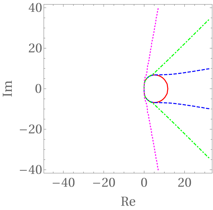
(b) ESDIRK2(1)3

(c) SDIRK3(2)4

(d) ESDIRK3(2)4

(e) SDIRK4(3)5

(f) ESDIRK4(3)6

Figure 5: Scalar stability regions $\mathcal{S}^{\textsc{1d}}_{\infty,\alpha}$ for SPC-MRI-GARK methods

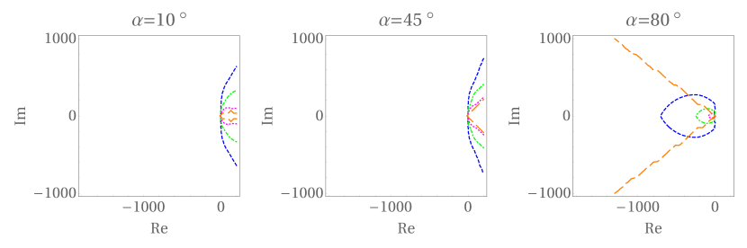
(a) SDIRK2(1)2

(b) ESDIRK2(1)3

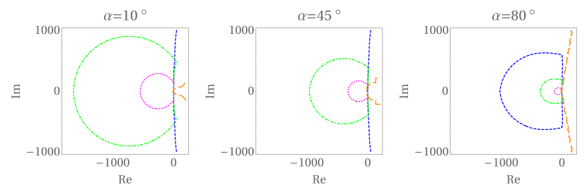
(c) SDIRK3(2)4

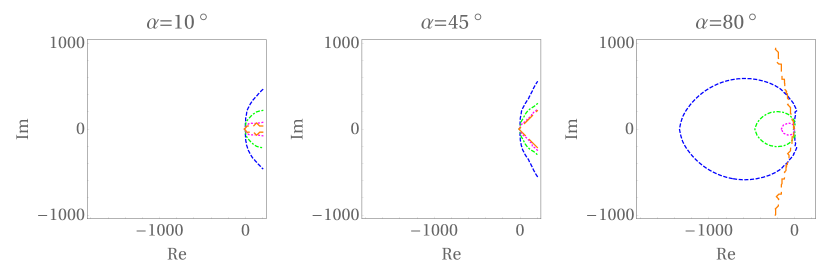
(a) ESDIRK3(2)4

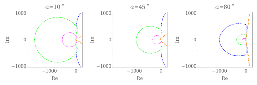
(b) SDIRK4(3)5

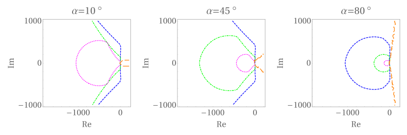
(c) ESDIRK4(3)6

Figure 7: Matrix stability regions $\mathcal{S}^{\textsc{2d}}_{\infty,\alpha}$ for SPC-MRI-GARK methods

A.2 IPC-MRI-GARK methods

We will using the following tableau representation for IPC-MRI-GARK methods:

A.2.1 SDIRK2(1)2

This method is based on the two stage, second order method in [1].

$$\begin{array}[]{c|cc|cc}{\scriptstyle 1-}\frac{1}{\sqrt{2}}&{\scriptstyle 0}&{\scriptstyle 0}&{\scriptstyle 1-}\frac{1}{\sqrt{2}}&{\scriptstyle 0}\\ {\scriptstyle 1}&\frac{1}{\sqrt{2}}&{\scriptstyle 0}&\frac{1}{\sqrt{2}}{\scriptstyle-1}&{\scriptstyle 1-}\frac{1}{\sqrt{2}}\\ \hline\cr\text{}&\frac{3}{5}&{\scriptstyle 0}&\frac{1}{\sqrt{2}}{\scriptstyle-1}&\frac{2}{5}\\ \end{array}$$

A.2.2 ESDIRK2(1)3

This method is based on TR-BDF2 in [5].

$$\begin{array}[]{c|ccc|ccc}{\scriptstyle 0}&{\scriptstyle 0}&{\scriptstyle 0}&{\scriptstyle 0}&{\scriptstyle 0}&{\scriptstyle 0}&{\scriptstyle 0}\\ {\scriptstyle 2-\sqrt{2}}&{\scriptstyle 1-}\frac{1}{\sqrt{2}}&{\scriptstyle 0}&{\scriptstyle 0}&{\scriptstyle 0}&{\scriptstyle 1-}\frac{1}{\sqrt{2}}&{\scriptstyle 0}\\ {\scriptstyle 1}&\frac{3}{2\sqrt{2}}{\scriptstyle-1}&\frac{1}{2\sqrt{2}}&{\scriptstyle 0}&{\scriptstyle 0}&\frac{1}{\sqrt{2}}{\scriptstyle-1}&{\scriptstyle 1-}\frac{1}{\sqrt{2}}\\ \hline\cr\text{}&\frac{1}{\sqrt{2}}-\frac{7}{10}&\frac{3}{10}&{\scriptstyle 0}&{\scriptstyle 0}&\frac{1}{\sqrt{2}}{\scriptstyle-1}&\frac{2}{5}\\ \end{array}$$

A.2.3 SDIRK3(2)5

$$\begin{array}[]{c|ccccc|ccccc}\frac{7}{40}&{\scriptstyle 0}&{\scriptstyle 0}&{\scriptstyle 0}&{\scriptstyle 0}&{\scriptstyle 0}&\frac{7}{40}&{\scriptstyle 0}&{\scriptstyle 0}&{\scriptstyle 0}&{\scriptstyle 0}\\ \frac{1}{3}&\frac{19}{120}&{\scriptstyle 0}&{\scriptstyle 0}&{\scriptstyle 0}&{\scriptstyle 0}&-\frac{7}{40}&\frac{7}{40}&{\scriptstyle 0}&{\scriptstyle 0}&{\scriptstyle 0}\\ \frac{1}{3}&\frac{1}{10}&-\frac{1}{10}&{\scriptstyle 0}&{\scriptstyle 0}&{\scriptstyle 0}&{\scriptstyle 0}&-\frac{7}{40}&\frac{7}{40}&{\scriptstyle 0}&{\scriptstyle 0}\\ {\scriptstyle 1}&\frac{17341}{182400}&-\frac{73}{70}&\frac{687111}{425600}&{\scriptstyle 0}&{\scriptstyle 0}&{\scriptstyle 0}&{\scriptstyle 0}&-\frac{7}{40}&\frac{7}{40}&{\scriptstyle 0}\\ {\scriptstyle 1}&-\frac{21487}{60800}&\frac{1618427}{1702400}&-\frac{1144471}{1702400}&\frac{3}{40}&{\scriptstyle 0}&{\scriptstyle 0}&{\scriptstyle 0}&{\scriptstyle 0}&-\frac{7}{40}&\frac{7}{40}\\ \hline\cr\text{}&\frac{2833}{60800}&-\frac{9}{35}&\frac{17257}{425600}&\frac{1}{6}&{\scriptstyle 0}&{\scriptstyle 0}&{\scriptstyle 0}&{\scriptstyle 0}&-\frac{7}{40}&\frac{107}{600}\\ \end{array}$$

A.2.4 SDIRK4(3)6

A.2.5 Stability plots

Figures 8 and 9 show the scalar and matrix stability regions, respectively.

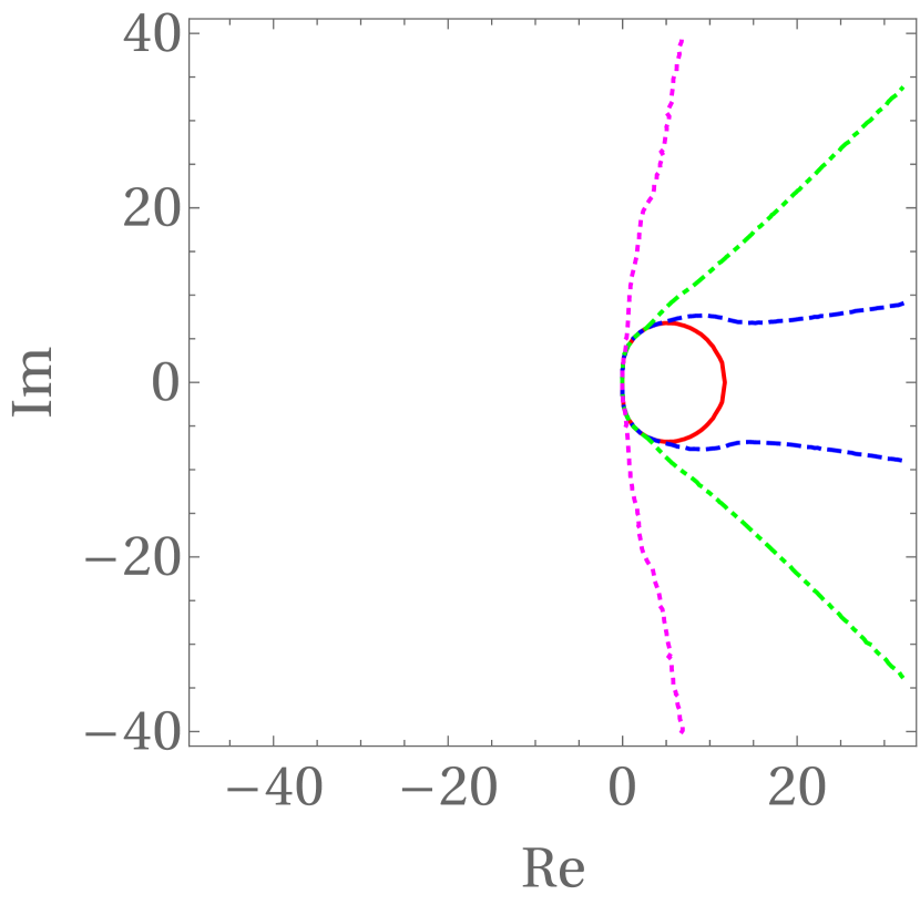
(a) SDIRK2(1)2

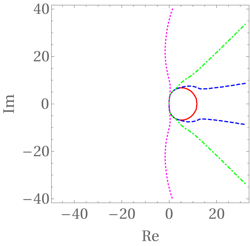
(b) ESDIRK2(1)3

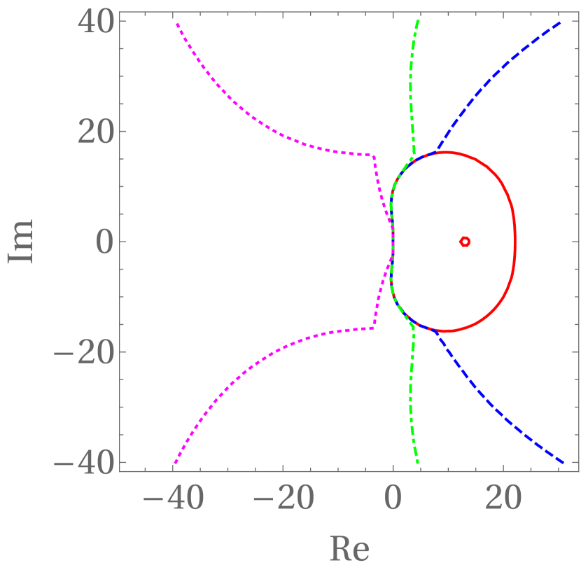
(c) SDIRK3(2)5

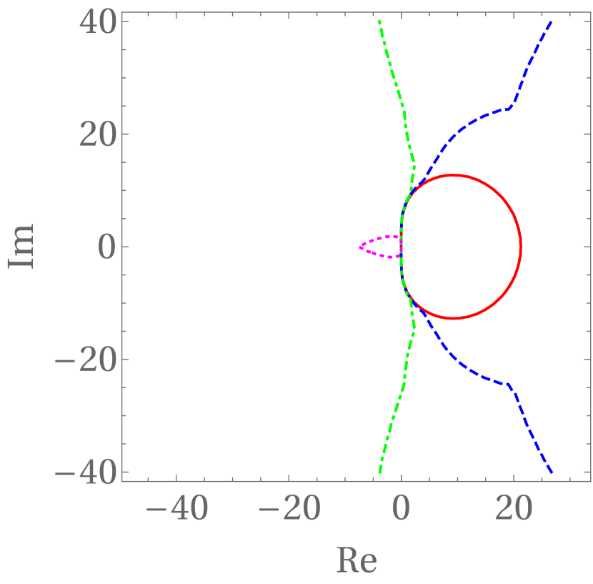
(d) SDIRK4(3)6

Figure 8: Scalar stability regions $\mathcal{S}^{\textsc{1d}}_{\infty,\alpha}$ for IPC-MRI-GARK methods

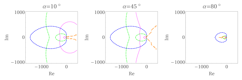
(a) SDIRK2(1)2

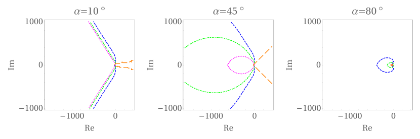
(b) ESDIRK2(1)3

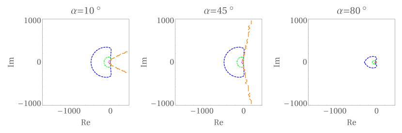
(c) SDIRK3(2)5

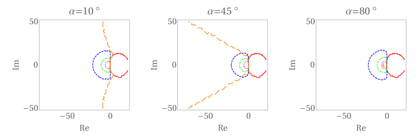
(d) SDIRK4(3)6

Figure 9: Matrix stability regions $\mathcal{S}^{\textsc{2d}}_{\infty,\alpha}$ for IPC-MRI-GARK methods

References

• [1] R. Alexander, Diagonally implicit Runge–Kutta methods for stiff ODE’s, SIAM Journal on Numerical Analysis, 14 (1977), pp. 1006–1021.
• [2] J. Andrus, Numerical solution for ordinary differential equations separated into subsystems, SIAM Journal on Numerical Analysis, 16 (1979), pp. 605–611.
• [3] J. Andrus, Stability of a multirate method for numerical integration of ODEs, Computers Math. Applic, 25 (1993), pp. 3–14.
• [4] A. L. Araujo, A. Murua, and J. M. Sanz-Serna, Symplectic methods based on decompositions, SIAM Journal on Numerical Analysis, 34 (1997), pp. 1926–1947.
• [5] R. E. Bank, W. M. Coughran, W. Fichtner, E. H. Grosse, D. J. Rose, and R. K. Smith, Transient simulation of silicon devices and circuits, IEEE Transactions on Computer-Aided Design of Integrated Circuits and Systems, 4 (1985), pp. 436–451, https://doi.org/10.1109/TCAD.1985.1270142.
• [6] A. Bartel and M. Günther, A multirate W-method for electrical networks in state-space formulation, Journal of Computational Applied Mathematics, 147 (2002), pp. 411–425, https://doi.org/10.1016/S0377-0427(02)00476-4.
• [7] E. Constantinescu and A. Sandu, Multirate timestepping methods for hyperbolic conservation laws, Journal on Scientific Computing, 33 (2007), pp. 239–278, https://doi.org/10.1007/s10915-007-9151-y.
• [8] E. Constantinescu and A. Sandu, Extrapolated multirate methods for differential equations with multiple time scales, Journal of Scientific Computing, 56 (2013), pp. 28–44, https://doi.org/10.1007/s10915-012-9662-z.
• [9] B. Engquist and R. Tsai, Heterogeneous multiscale methods for stiff ordinary differential equations, Mathematics of Computation, 74 (2005), pp. 1707–1742.
• [10] C. Engstler and C. Lubich, Multirate extrapolation methods for differential equations with different time scales, Computing, 58 (1997), pp. 173–185, https://doi.org/10.1007/BF02684438.
• [11] C. Gear and D. Wells, Multirate linear multistep methods, BIT, 24 (1984), pp. 484–502.
• [12] M. Günther and M. Hoschek, ROW methods adapted to electric circuit simulation packages, Journal of computational and applied mathematics, 82 (1997), pp. 159–170.
• [13] M. Günther, A. Kværnø, and P. Rentrop, Multirate partitioned Runge–Kutta methods, BIT Numerical Mathematics, 41 (2001), pp. 504–514, https://doi.org/10.1023/A:1021967112503.
• [14] M. Günther and P. Rentrop, Partitioning and multirate strategies in latent electric circuits, Birkhäuser Basel, Basel, 1994, pp. 33–60, https://doi.org/10.1007/978-3-0348-8528-7_3.
• [15] M. Günther and A. Sandu, Multirate generalized additive Runge–Kutta methods, Numerische Mathematik, 133 (2016), pp. 497–524, https://doi.org/10.1007/s00211-015-0756-z.
• [16] E. Hairer, S. Norsett, and G. Wanner, Solving ordinary differential equations I: Nonstiff problems, no. 8 in Springer Series in Computational Mathematics, Springer-Verlag Berlin Heidelberg, 1993.
• [17] E. Hairer and G. Wanner, Solving ordinary differential equations II: Stiff and differential-algebraic problems, no. 14 in Springer Series in Computational Mathematics, Springer-Verlag Berlin Heidelberg, 2 ed., 1996.
• [18] T. Kato and T. Kataoka, Circuit analysis by a new multirate method, Electrical Engineering in Japan, 126 (1999), pp. 55–62.
• [19] C. A. Kennedy and M. H. Carpenter, Diagonally implicit Runge–Kutta methods for ordinary differential equations. A review, Tech. Report NASA/TM-2016-219173, NASA, 2016.
• [20] C. A. Kennedy and M. H. Carpenter, Diagonally implicit Runge–Kutta methods for stiff ODEs, Applied Numerical Mathematics, 146 (2019), pp. 221 – 244, https://doi.org/10.1016/j.apnum.2019.07.008.
• [21] O. Knoth and J. Wensch, Generalized split-explicit Runge–Kutta methods for the compressible Euler equations, Monthly Weather Review, 142 (2014).
• [22] O. Knoth and R. Wolke, Implicit-explicit Runge–Kutta methods for computing atmospheric reactive flows, Applied Numerical Mathematics, 28 (1998).
• [23] A. Kværnø, Stability of multirate Runge–Kutta schemes, International Journal of Differential Equations and Applications, 1 (2000), pp. 97–105.
• [24] A. Kværnø and P. Rentrop, Low order multirate Runge–Kutta methods in electric circuit simulation, 1999, citeseer.ist.psu.edu/629589.html.
• [25] A. Logg, Multi-adaptive Galerkin methods for ODEs I, SIAM Journal on Scientific Computing, 24 (2003), pp. 1879–1902.
• [26] J. E. Pearson, Complex patterns in a simple system, Science, 261 (1993), pp. 189–192, https://doi.org/10.1126/science.261.5118.189.
• [27] A. Prothero and A. Robinson, On the stability and accuracy of one-step methods for solving stiff systems of ordinary differential equations, Mathematics of Computation, 28 (1974), pp. 145–162.
• [28] J. Rice, Split Runge–Kutta methods for simultaneous equations, Journal of Research of the National Institute of Standards and Technology, 60 (1960).
• [29] S. Roberts, J. Loffeld, A. Sarshar, C. S. Woodward, and A. Sandu, Implicit multirate GARK methods, arXiv preprint arXiv:1910.14079, (2019).
• [30] A. Sandu, A class of multirate infinitesimal GARK methods, SIAM Journal on Numerical Analysis, 57 (2019), pp. 2300–2327, https://doi.org/10.1137/18M1205492.
• [31] A. Sandu and E. Constantinescu, Multirate Adams methods for hyperbolic equations, Journal of Scientific Computing, 38 (2009), pp. 229–249, https://doi.org/doi:10.1007/s10915-008-9235-3.
• [32] A. Sandu and M. Günther, A generalized-structure approach to additive Runge–Kutta methods, SIAM Journal on Numerical Analysis, 53 (2015), pp. 17–42, https://doi.org/10.1137/130943224.
• [33] A. Sarshar, S. Roberts, and A. Sandu, Design of high-order decoupled multirate GARK schemes, SIAM Journal on Scientific Computing, 41 (2019), pp. A816–A847, https://doi.org/10.1137/18M1182875.
• [34] V. Savcenko, Comparison of the asymptotic stability properties for two multirate strategies, Tech. Report MAS-R0705, CWI, Amsterdam, 2007.
• [35] V. Savcenko, W. Hundsdorfer, and J. Verwer, Multirate time-stepping methods for hyperbolic conservation laws, BIT Numer. Math., 47 (2007), pp. 137–155.
• [36] M. Schlegel, O. Knoth, M. Arnold, and R. Wolke, Multirate Runge–Kutta schemes for advection equations, Journal of Computational and Applied Mathematics, 226 (2009), pp. 345–357.
• [37] M. Schlegel, O. Knoth, M. Arnold, and R. Wolke, Multirate implicit-explicit time integration schemes in atmospheric modelling, in AIP Conference Proceedings, vol. 1281, International Conference of Numerical Analysis and Applied Mathematics, 2010, pp. 1831–1834.
• [38] M. Schlegel, O. Knoth, M. Arnold, and R. Wolke, Implementation of splitting methods for air pollution modeling, Geoscientific Model Development Discussions, 4 (2011), pp. 2937–2972.
• [39] J. M. Sexton and D. R. Reynolds, Relaxed multirate infinitesimal step methods, arXiv preprint arXiv:1808.03718, (2018).
• [40] J. Wensch, O. Knoth, and A. Galant, Multirate infinitesimal step methods for atmospheric flow simulation, BIT Numerical Mathematics, 49 (2009), pp. 449–473.