Mean escape time for randomly switching narrow gates in a cellular flow

Abstract

The escape of particles through a narrow absorbing gate in confined domains is a abundant phenomenon in various systems in physics, chemistry and molecular biophysics. We consider the narrow escape problem in a cellular flow when the two gates randomly switch between different states with a switching rate $k$ between the two gates. After briefly deriving the coupled partial differential equations for the escape time through two gates, we compute the mean escape time for particles escaping from the gates with different initial states. By numerical simulation under nonuniform boundary conditions, we quantify how narrow escape time is affected by the switching rate $k$ between the two gates, arc length $s$ between two gates, angular velocity $w$ of the cellular flow and diffusion coefficient $D$. We reveal that the mean escape time decreases with the switching rate $k$ between the two gates, angular velocity $w$ and diffusion coefficient $D$ for fixed arc length, but takes the minimum when the two gates are evenly separated on the boundary for any given switching rate $k$ between the two gates. In particular, we find that when the arc length size $\varepsilon$ for the gates is sufficiently small, the average narrow escape time is approximately independent of the gate arc length size. We further indicate combinations of system parameters (regions located in the parameter space) such that the mean escape time is the longest or shortest. Our findings provide mathematical understanding for phenomena such as how ions select ion channels and how chemicals leak in annulus ring containers, when drift vector fields are present.

Key words: Narrow escape; Brownian motion; small gate; mixed boundary conditions; biophysical modeling.

1 Introduction

The narrow escape problems have attracted a lot of attention in recent years, due to its significant relevance in cellular and molecular biology, and chemical physics [1, 2, 3, 4, 5, 6]. The heart of a narrow escape problem is to compute the narrow escape time (NET), namely the mean time for a particle starting in the domain before exiting through a narrow gate on the boundary.

In the biophysics context, when an ion searches for an open ion channel within the membrane, neurotransmitter receptors transmit signal within a synapse of a neuron, a reactive particle to activate a given protein, or newly transcribed mRNA transports from the nucleus to the cytoplasm through nuclear pores [7, 8, 9]. These examples have something in common: ‘Particles’ are all confined to a bounded domain with small exits (or holes, or gates) on the boundary of the domain. Meanwhile, in order to fulfill their biological function, particles must exit from the small gates on the boundary. For instance, viruses must enter the cell nucleus through small nanopores in order to replicate [10].

The narrow escape problems have been studied via various stochastic models recently. Most of the scenarios considered are two-dimensional [11, 12, 13, 14, 15], and some are one-dimensional [16, 17] or three-dimensional [17, 18, 19]. In addition, some authors consider the boundary with one gate [7, 20, 21, 22], with two gates[16, 20], while others multiple gates [10, 20, 23].

Several papers [14, 17, 18, 24, 25] have been devoted to the asymptotic approximate expressions for the narrow escape time. Since the mixed boundary conditions, there is no exact solution for a narrow escape problem. The narrow escape problems are mostly studied analytically [12, 14, 15, 16, 18, 20, 21, 23, 26, 27, 28, 29, 30, 31, 32]. For example, a general exact formula for the mean first passage time from a fixed point inside a planar domain to an escape region on its boundary is attained in [12]; high-order asymptotic formulas for the mean first passage time are derived in [14]; approximations for the average mean first passage time are found in[18]; the upper and lower bounds of the mean first passage time for mortal walkers are derived in[26]. Moreover, a spectral approach to derive an exact formula for the mean exit time of a particle through a hole on the boundary is developed in[27]; partial differential equation and probabilistic methods are applied to solve escape problems in [28]; a generalized Kramers formula for the mean escape time through a narrow window is obtained in[30]; and boundary homogenization is used when the boundary contains non-overlapping identical absorbing arcs in [31].

A few authors numerically studied the narrow escape problems, including Brownian simulations [17] and Monte Carlo simulations [33]. Think of the narrow escape problem the other way around, Agranov and Meerson [22] developed a formalism to evaluate the nonescape probability of a gas of diffusing particles.

Most works approximately estimate the narrow escape time of particles under Brownian diffusion (i.e., no drift or no external vector field). It turns out that the escape time is described by a mixed Dirichlet-Neumann boundary value problem for the Laplace operator in a bounded domain [1, 34]. Very recently, Lagache and Holcman [10] considered the narrow escape problem for particles in a constant drift, in order to analyze viral entry into the cell nucleus.

In this paper, we consider a two dimensional model of narrow escape problem for particles in a unit annulus, with two randomly switching gates on the outer boundary, under a vector field (i.e., a cellular flow). The circular annulus may represent the cell cytoplasm, with outer radius $r_{2}$ and inner radius $r_{1}$. The two dimensional model may represent flat culture cells. Since the adhesion to the substrate, they stay flat. The thickness can be neglected in this idealized model.

This paper is organized as follows. In Section 2, we first describe a stochastic narrow escape model, then briefly drive the coupled partial differential equations to be satisfied by the mean escape time through two gates. In Section 3, we present numerical experiments and analysis. We end the paper with a discussion in Section 4.

2 Materials and methods

2.1 Stochastic narrow escape model

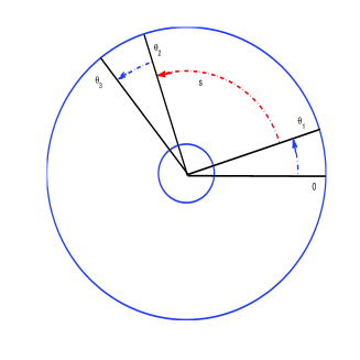
Figure 1: (Color online) A unit annular domain with small absorbing gates on an otherwise reflecting outer circular boundary.

We consider particles moving in an annular domain with inner radius $r_{1}$ and outer radius $r_{2}$, in a cellular flow. The steady cellular flow [35] is induced by the rotation of the inner boundary with angular velocity $w$, and is expressed in polar coordinates as $(0,Ar+\frac{B}{r})$ with

$$A=\frac{-wr_{1}^{2}}{r_{2}^{2}-r_{1}^{2}},$$ (1)

$$B=\frac{wr_{1}^{2}r_{2}^{2}}{r_{2}^{2}-r_{1}^{2}}.$$ (2)

By the transformation of polar coordinates, $x=r\cos\theta$, $y=r\sin\theta$ with $r=\sqrt{x^{2}+y^{2}}$, the cellular flow in the Cartesian coordinates is

$$b_{1}(x,y)=-y\frac{-wr_{1}^{2}(x^{2}+y^{2})+wr_{1}^{2}r_{2}^{2}}{\sqrt{x^{2}+y^{2}}(r_{2}^{2}-r_{1}^{2})},$$ (3)

$$b_{2}(x,y)=x\frac{-wr_{1}^{2}(x^{2}+y^{2})+wr_{1}^{2}r_{2}^{2}}{\sqrt{x^{2}+y^{2}}(r_{2}^{2}-r_{1}^{2})}.$$ (4)

With the driving cellular flow $b(x,y):=(b_{1}(x,y),b_{2}(x,y))$, we consider the two dimensional domain $\Omega$, whose boundary is decomposed as $\partial\Omega=\partial\Omega_{c}\bigcup\partial\Omega_{1}\bigcup\partial\Omega_{2}$. The boundary has two small gates at the arcs $\partial\Omega_{1}$ and $\partial\Omega_{2}$, together with the remaining part $\Omega_{c}$. A particle’s trajectory is reflected on $\Omega_{c}$, but absorbed at gates $\Omega_{1}$ or $\Omega_{2}$. Each gate is a small absorbing arc. We consider the following stochastic narrow escape model, i.e., the equations of motion for a particle

$$\begin{cases}dx_{t}&=b_{1}(x_{t},y_{t})dt+\sqrt{2D}dB_{t}^{1}-n_{1}(x_{t},y_{t})dL_{t},\\ dy_{t}&=b_{2}(x_{t},y_{t})dt+\sqrt{2D}dB_{t}^{2}-n_{2}(x_{t},y_{t})dL_{t},\end{cases}$$ (5)

where $(b_{1}(x,y),b_{2}(x,y))$ is a drift vector field (a cellular flow), $(B_{t})_{t\geq 0}=(B_{t}^{1},B_{t}^{2})$ is a standard Brownian motion, $n=(n_{1},n_{2})$ is the outward unit normal vector on the boundary, $(L_{t})_{t\geq 0}$ is a continuous nondecreasing process (with $L_{0}=0$) which increases only when $(x,y)$ is on the boundary $\partial\Omega$:

$$L_{t}=\int_{0}^{t}\mathbb{I}_{(x,y)\in\partial\Omega}dL_{s}.$$ (6)

Assume that the two gates at the arcs $\partial\Omega_{1}$ and $\partial\Omega_{2}$ open alternatively [11, 15] in terms of a telegraph process $(N_{t})_{t\geq 0}$ with parameter $k$, where $k$ is the rate of switching between the two gates. When the particle in the cytoplasm hits the open gate it escapes, if not it will be reflected. The telegraph process $(N_{t})_{t\geq 0}$ with parameter $k$ is a Markov process which takes on only two values, $1$ and $2$. The different values of Markov process corresponding to different states, different function of cell [36]. The process can be described as follows

$$N_{t}=\left\{\begin{array}[]{ll}1,&\hbox{if $T_{2j}\leq t<T_{2j+1}$ for some $j$,}\\ 2,&\hbox{if $T_{2j+1}\leq t<T_{2j+2}$ for some $j$,}\end{array}\right.$$

where $T_{0}=0$, $T_{j}=\sum_{l=1}^{j}\tau_{l}$, and $\tau_{l}$ is a sequence of independent and identically distributed exponential random variables with parameter $k>0$. That is, $\mathbb{E}[\tau_{l}]=\frac{1}{k}$. Denote $\textbf{X}_{t}=(x_{t},y_{t})$ and $\textbf{x}=(x,y)$. We denote $\mathcal{T}$ as the stopping time corresponding to the escape of the particle: $\mathcal{T}=\mathcal{T}_{1}\wedge\mathcal{T}_{2}$, $\mathcal{T}_{j}=\inf\{t\geq 0,N_{t}=j\ and\ \mathbf{X}_{t}\in\partial\Omega_{j}\}$, j=1, 2.

2.2 Narrow escape time with drift

Our goal is to compute the expected quantities $u_{1}(\textbf{x})=\mathbb{E}_{1,\textbf{x}}[\mathcal{T}]$ and $u_{2}(\textbf{x})=\mathbb{E}_{2,\textbf{x}}[\mathcal{T}]$ of the stopping time given the initial state is $N_{0}=j$ and $\mathbf{X}_{0}=\mathbf{x}$, j=1, 2.

More specifically, $u_{1}(x,y)$ is the mean time that the particle starting at $(x,y)$ in the domain escape from any gate with the first gate open initially. Similarly, $u_{2}(x,y)$ is the mean time that the particle starting at $(x,y)$ in the domain escape from any gate with the second gate open initially. We now prove the following theorem.

Theorem 1.

The mean narrow escape times $u_{1},u_{2}$ satisfy the following coupled partial differential equations

$$-\begin{pmatrix}1\\ 1\end{pmatrix}=k\begin{pmatrix}-1&1\\ 1&-1\end{pmatrix}\begin{pmatrix}u_{1}(x,y)\\ u_{2}(x,y)\end{pmatrix}+D\Delta\begin{pmatrix}u_{1}(x,y)\\ u_{2}(x,y)\end{pmatrix}+\begin{pmatrix}b\cdot\nabla u_{1}(x,y)\\ b\cdot\nabla u_{2}(x,y)\end{pmatrix}$$ (7)

with nonuniform boundary conditions:

$$\partial_{n}u_{j}|_{\partial\Omega_{c}}=0,j=1,2,$$ (8)

$$u_{1}|_{\partial\Omega_{1}}=0,u_{2}|_{\partial\Omega_{2}}=0,$$ (9)

$$\partial_{n}u_{1}|_{\partial\Omega_{2}}=0,\partial_{n}u_{2}|_{\partial\Omega_{1}}=0,$$ (10)

where $\partial_{n}$ represents the normal derivative and $n$ is outward unit normal vector on the outer boundary.

Proof.

Note that the right-hand side of the (7) is the infinitesimal generator $\mathcal{A}$ of the process $(\mathbf{X}_{t},N_{t})_{t\geq 0}$. Denoting $u(\mathbf{x},j)=u_{j}(\mathbf{x})$, by Itô formula [37], we have the following relation, for $s<t$,

$$\mathbb{E}[u(\mathbf{X}_{t\wedge\mathcal{T}},N_{t\wedge\mathcal{T}})-u(\mathbf{X}_{s\wedge\mathcal{T}},N_{s\wedge\mathcal{T}})-\int_{s\wedge\mathcal{T}}^{t\wedge\mathcal{T}}\mathcal{A}u(\mathbf{X}_{r},N_{r})dr|\mathcal{F}_{s\wedge\mathcal{T}}]$$ (11)

$$= -\mathbb{E}[\int_{s\wedge\mathcal{T}}^{t\wedge\mathcal{T}}\partial_{\nu}u(\mathbf{X}_{r},N_{r})dL_{r}|\mathcal{F}_{s\wedge\mathcal{T}}]+\mathbb{E}[\int_{s\wedge\mathcal{T}}^{t\wedge\mathcal{T}}\nabla u(\mathbf{X}_{r},N_{r})\sqrt{2D}dB_{r}|\mathcal{F}_{s\wedge\mathcal{T}}]$$

$$= -\mathbb{E}[\int_{s\wedge\mathcal{T}}^{t\wedge\mathcal{T}}\partial_{\nu}u(\mathbf{X}_{r},N_{r})dL_{r}|\mathcal{F}_{s\wedge\mathcal{T}}]$$

where $(\mathcal{F}_{t})_{t\geq 0}$ is the filtration of the process $(\mathbf{X}_{t},N_{t})_{t\geq 0}$, and $L_{t}$ is defined as above. Neumann boundary conditions (8) and (10) show us that $\partial_{\nu}u(\mathbf{X}_{r},N_{r})=0$ if $r<\mathcal{T}$. By the given condition, we know $\mathcal{A}u(\mathbf{X}_{r},N_{r})=-1$. This leads to

$$\mathbb{E}[u(\mathbf{X}_{t\wedge\mathcal{T}},N_{t\wedge\mathcal{T}})-u(\mathbf{X}_{s\wedge\mathcal{T}},N_{s\wedge\mathcal{T}})+(t\wedge\mathcal{T}-s\wedge\mathcal{T})|\mathcal{F}_{s\wedge\mathcal{T}}]=0,$$

which means the process $(u(\mathbf{X}_{t\wedge\mathcal{T}},N_{t\wedge\mathcal{T}})+t\wedge\mathcal{T})_{t\geq 0}$ is a martingale. Then applying this equality with $s=0$ and letting $t\rightarrow\infty$, we get

$$\mathbb{E}[u(\mathbf{X}_{\mathcal{T}},N_{\mathcal{T}})-u(\mathbf{X}_{0},N_{0})+\mathcal{T}|\mathcal{F}_{0}]=0.$$

From the Dirichlet boundary conditions in (9), we have $u(\mathbf{X}_{\mathcal{T}},N_{\mathcal{T}})=0$. Thus we obtain

$$\mathbb{E}[\mathcal{T}|\mathcal{F}_{0}]=\mathbb{E}[u(\mathbf{X}_{0},N_{0})|\mathcal{F}_{0}].$$ (12)

Finally, we take the expectation of both sides of the equation (12),

$$\mathbb{E}_{k,\mathbf{x}}\mathcal{T}=\mathbb{E}u(\mathbf{x}_{0},N_{0})=\mathbb{E}u(\mathbf{x},k)=u_{k}(\mathbf{x}).$$

This gives the desired result when the initial distribution is such that $N_{0}=k$ and $\mathbf{X}_{0}=\mathbf{x}$. ∎

Note that Ammari et al. [11] showed this theorem in the case of no drift.

In the polar coordinates, the NET $u(r,\theta)$ is the solution of the preceding boundary value problem given the initial point $(r,\theta)$. It is a reflected diffusion process to the absorbing boundary $\partial\Omega_{j},(j=1,2)$. In the context of polar coordinates: $x=r\cos\theta$, $y=r\sin\theta$, we obtain that

$$\partial_{\nu}u=\partial_{x}u\cos\theta+\partial_{y}u\sin\theta=0,$$ (13)

$$\partial_{x}u=\partial_{r}u\partial_{x}r+\partial_{\theta}u\partial_{x}\theta=\cos\theta\partial_{r}u-\frac{\sin\theta}{r}\partial_{\theta}u,$$ (14)

$$\partial_{y}u=\partial_{r}u\partial_{y}r+\partial_{\theta}u\partial_{y}\theta=\sin\theta\partial_{r}u+\frac{\cos\theta}{r}\partial_{\theta}u,$$ (15)

and

$$\Delta u=\partial_{xx}u+\partial_{yy}u=\partial_{rr}u+\frac{1}{r^{2}}\partial_{\theta\theta}u+\frac{1}{r}\partial_{r}u.$$ (16)

We use a finite difference method to solve the Dirichlet-Neumann boundary value problem (7)-(10) in the polar coordinates.

3 Results and Discussion

We now describe our numerical simulation results of the narrow escape time (NET). The Dirichlet-Neumann boundary value problem in Theorem 1 is solved by a finite difference method. The goal here is to present the results for the averaged NET from the numerical simulation, then conduct comparisons for different parameters.

The average NET is the average escape time that all the particles in the annular domain take to escape the annular domain from any gate. It is also called average mean first passage time [38, 39]. In the context of polar coordinates, the average NET is given by

$$\frac{1}{\pi(r_{2}^{2}-r_{1}^{2})}\int\int_{\Omega^{\prime}}u(r,\theta)drd\theta,$$ (17)

where $\Omega^{\prime}=[r_{1},r_{2}]\times[0,2\pi]$.

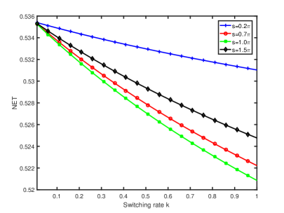
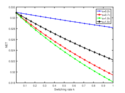
Figure 2: (Color online) Average narrow escape time with switching rate $k$ between the two gates for diffusion coefficient $D=1$ and angular velocity $w=3$: (a) With the first gate open initially. (b) With the second gate open initially.

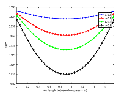
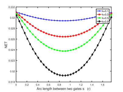
Figure 3: (Color online) Average narrow escape time with the arc length $s$ between two gates for diffusion coefficient $D=1$ and angular velocity $w=3$: (a) With the first gate open initially. (b) With the second gate open initially.

First, we show the relationship of average NET with switching rate $k$ between the two gates and arc length (‘distance’) $s$ between two gates in Fig 2 and Fig 3.

In Fig 2, the average NET is plotted as a function of switching rate between the two gates $k$. We compare average NET for different arc length $s$ between two gates. when the arc length between two gates $0<s\leq\pi$, the average NET decreases with the increase of arc length $s$ between two gates , while for $\pi<s<2\pi$, the average NET is longer than that of $s=\pi$. To understand the reason for this at $s=\pi$, note that the two gates are evenly distributed on the cell boundary, so the particle may choose the nearest side to escape quickly; but for $0<s<\pi$ or $\pi<s<2\pi$, the two gates are on the same side of the semicircle, thus the particle in the other semicircle has to cross over to the other side then escape. Fig 3 plots the effects of arc length $s$ between two gates on average NET for various switching rate $k$ between the two gates. As we explained above, the average NET is smallest when arc length $s$ between two gates is around $\pi$. Meanwhile, Fig 2 and Fig 3 both suggest that the average NET decrease as the switching rate $k$ between the two gates increases, this is consistent with known theoretical result [11].

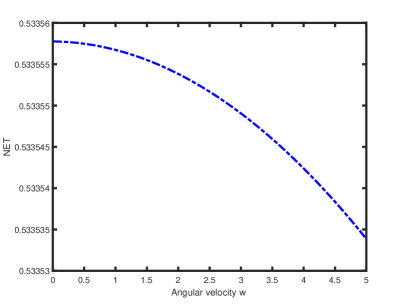
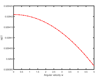
Figure 4: (Color online)Average narrow escape time with angular velocity $w$ for switching rate $k=0.1$ between the two gates, diffusion coefficient $D=1$ and arc length $s=\pi$ between two gates: (a)With the first gate open initially. (b) With the second gate open initially.

Each curve in Fig 4 predicts an decrease in the average NET with angular velocity $w$. We plot here for switching rate $k=0.1$ between the two gates, for $0<k<1$, it has similar trends.

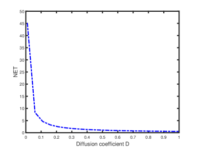
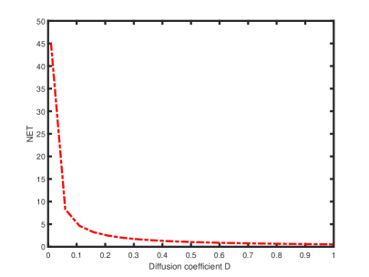
Figure 5: (Color online) Average narrow escape time with diffusion coefficient $D$ for switching rate $k=0.3$ between the two gates, angular velocity $w=3$ and arc length $s=\pi$ between two gates: (a) With the first gate open initially. (b) With the second gate open initially.

Fig 5 demonstrates that the effects of diffusion coefficient $D$ on the average NET. We see that the average NET has a monotonic behavior with the diffusion coefficient $D$. The average NET declines when $D$ is small, then when average NET crosses the inflection point, it changes more modestly. In this case, small diffusion coefficient $D$ is not good for particles to escape quickly.

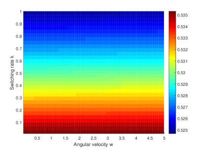
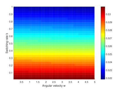
Figure 6: (Color online) Average narrow escape time with angular velocity $w$ and switching rate $k$ between the two gates for diffusion coefficient $D=1$ and arc length $s=0.5\pi$ between two gates: (a) With the first gate open initially. (b) With the second gate open initially.

Fig 6 presents the combined effects of angular velocity $w$ and switching rate $k$ between the two gates on average NET. In both Fig 6(a) and Fig 6(b), the red region presents the larger average NET domain, while the blue region represents the smaller parts. The smaller average NET values occur when $(w,k)$ is in the blue domains at the top. Different initial states have very little influence on average NET.

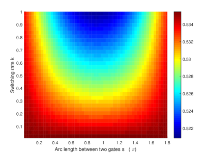
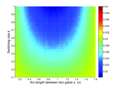
Figure 7: (Color online) Average narrow escape time with the arc length $s$ between two gates and switching rate $k$ between the two gates for diffusion coefficient $D=1$ and angular velocity $w=3$ : (a) With the first gate open initially. (b) With the second gate open initially.

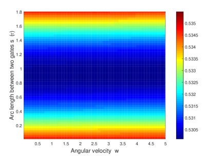
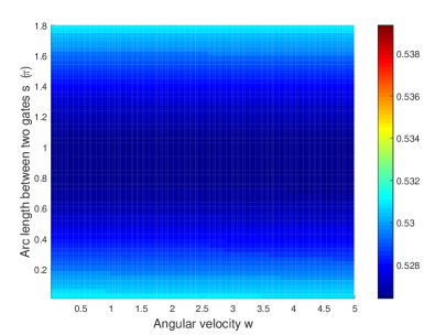
Figure 8: (Color online) Average narrow escape time with the arc length $s$ between two gates and angular velocity $w$ for diffusion coefficient $D=1$ and switching rate $k=0.5$ between the two gates: (a) With the first gate open initially. (b) With the second gate open initially.

In Fig 7, we display average NET as a function of arc length $s$ between two gates and switching rate $k$ between the two gates. Interestingly, we find that the average NET $u_{1}$ is larger than $u_{2}$ in many domains. If the initial state with the first gate open, escape from the first gate takes longer time than from the second gate. Similarly, we show the effects of arc length $s$ between two gates and angular velocity $w$ on average NET in Fig 8. We find a counterintuitive phenomenon, when the initial state is that the second gate is open, escape from the second gate is faster than from the first gate.

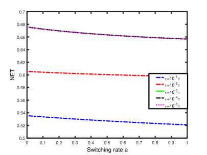
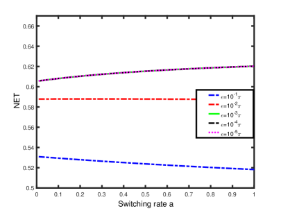
Figure 9: (Color online) Average narrow escape time with the switching rate $k$ between the two gates for diffusion coefficient $D=1$, angular velocity $w=3$ and arc length $s=\pi$ between two gates for different size of gates: (a) With the first gate open initially. (b) With the second gate open initially.

Fig 9 shows the effects of the gate arc length size $\varepsilon$ on average NET. As expected, the average NET decreases with the switching rate $k$ between the two gates, but when $\varepsilon$ is sufficiently small, the average NET is independent of gate arc length size $\varepsilon$.

4 Conclusion

In this work , we have analysed the average narrow escape time through two randomly switching gates in an annular domain, under a drift or a vector field, while most existing works are for particles following Brownian diffusion (i.e., no drift). We have conducted numerical experiments to reveal escape time’s dependence on angular velocity $w$ for the background cellular flow, switching rate $k$ between the two gates, diffusion coefficient $D$, arc length distance $s$ between two gates, and gate arc length size $\varepsilon$.

We have found that the mean escape time decreases with the switching rate $k$ between the two gates, angular velocity $w$ and diffusion coefficient $D$ for fixed arc length, but takes the minimum when the two gates are evenly separated on the boundary for given switching rate $k$ between the two gates. In particular, we have verified that when the arc length size $\varepsilon$ for the gates is sufficiently small, the average narrow escape time is independent of the gate arc length size. Our approach selects combinations of system parameters (located in the parameter space) such that the mean escape time is the longest or shortest.

The narrow escape problems are relevant in certain crucial processes in chemical physics and cellular biology. Our research sheds some lights on the narrow escape time in a vector field, when system parameters vary.

References

References

- [1] D. Holcman, Z. Schuss 2015 Stochastic Narrow Escape in Molecular and Cellular Biology: Analysis and Applications Springer New York
- [2] P. C. Bressloff 2014 Stochastic Processes in Cell Biology Springer New York
- [3] P. C. Bressloff, J. M. Newby 2013 Stochastic models of intracellular transport Reviews of Modern Physics 85(1) 135-196
- [4] D. Holcman, Z. Schuss 2017 100 years after Smoluchowski: stochastic processes in cell biology Journal of Physics A: Mathematical and Theoretical 50 093002
- [5] D. Holcman, Z. Schuss 2012 Brownian Motion in Dire Straits Siam Journal on Multiscale Modeling and Simulation 10(4) 1204-1231
- [6] J. Reingruber, D. Holcman 2009 Diffusion in narrow domains and application to phototransduction Physical Review E 79 030904
- [7] O. Bénichou, R. Voituriez 2008 Narrow-escape time problem: time needed for a particle to exit a confining domain through a small window Physical Review Letters 100 168105
- [8] Z. Schuss, A. Singer, D. Holcman 2007 The narrow escape problem for diffusion in cellular microdomains PNAS 104(41) 16098-16103
- [9] D. Holcman, Z. Schuss 2004 Escape Through a Small Opening: Receptor Trafficking in a Synaptic Membrane Journal of Statistical Physics 117 975-1014
- [10] T. Lagache, D. Holcman 2017 Extended Narrow Escape with Many Windows for Analyzing Viral Entry into the Cell Nucleus Journal of Statistical Physics 166 244 C266
- [11] H. Ammari, J. Garnier, H. Kang, H. Lee, K. Sølna 2011 The mean escape time for a narrow escape problem with multiple switching gates Multiscale Modeling and Simulation 9(2) 817 - 833
- [12] D. S. Grebenkov 2016 Universal Formula for the Mean First Passage Time in Planar Domains Physical Review Letters 117(26) 260201
- [13] X. Li 2014 Matched asymptotic analysis to solve the narrow escape problem in a domain with a long neck Journal of Physics A: Mathematical and Theoretical 47 505202
- [14] A. E. Lindsay, T. Kolokolnikov, J. C. Tzou 2015 Narrow escape problem with a mixed trap and the effect of orientation Physical Review E 91 032111
- [15] S. Pillay, M. J. Ward, A. Peirce, T. Kolokolnikov 2010 An Asymptotic Analysis of the Mean First Passage Time for Narrow Escape Problems: Part I: Two-Dimensional Domains Multiscale Modeling and Simulation 8 803-835
- [16] J. Reingruber, D. Holcman 2010 Narrow escape for a stochastically gated Brownian ligand Journal of Physics Condensed Matter 22 065103
- [17] J. Reingruber, D. Holcman 2009 Gated narrow escape time for molecular signaling Physical Review Letters 103 148102
- [18] D. Gomez, A. F. Cheviakov 2015 Asymptotic analysis of narrow escape problems in nonspherical three-dimensional domains Physical Review E 91 012137
- [19] X. Li, H. Lee, Y. Wang 2017 Asymptotic Analysis of the Narrow Escape Problem in Dendritic Spine Shaped Domain: Three Dimension Journal of Physics A: Mathematical and Theoretical 50 325203
- [20] C. Chevalier, O. Bénichou, B. Meyer, R. Voituriez 2011 First-passage quantities of Brownian motion in a bounded domain with multiple targets: a unified approach Journal of Physics A: Mathematical and Theoretical 44 025002
- [21] A. Singer, Z. Schuss, D. Holcman 2008 Narrow escape and leakage of Brownian particles Physical Review E 78 051111
- [22] T. Agranov, B. Meerson 2018 Narrow Escape of Interacting Diffusing Particles Physical Review Letters 12 120601
- [23] A. F. Cheviakov, A. S. Reimer, M. J. Ward 2012 Mathematical modeling and numerical computation of narrow escape problems Physical Review E 85 021131
- [24] D. Holcman, Z. Schuss 2013 Control of flux by narrow passages and hidden targets in cellular biology Reports on Progress in Physics Physical Society 76 074601
- [25] D. Holcman, Z. Schuss 2008 Diffusion escape through a cluster of small absorbing windows Journal of Physics A: Mathematical and Theoretical 41 155001
- [26] D. S. Grebenkov, J.-F. Rupprecht 2017 The escape problem for mortal walkers Journal of Chemical Physics 146 084106
- [27] O. Bénichou, D. S. Grebenkov, L. Hillairet, L. Phun, R. Voituriez, M. Zinsmeister 2015 Mean exit time for surface-mediated diffusion: spectral analysis and asymptotic behavior Analysis Mathematical Physics 5 321-362
- [28] P. C. Bressloff, S. D. Lawley 2015 Escape from Subcellular Domains with Randomly Switching Boundaries Multiscale Model. Simul. 13(4) 1420 C1445
- [29] F. Piazza, S. D. Traytak 2015 Diffusion-influenced reactions in a hollow nano-reactor with a circular hole Physical Chemistry Chemical Physics 17 10417-10425
- [30] A. Singer, Z. Schuss 2007 Activation through a narrow opening SIAM J. APPL. MATH. 68(1) 98 C108
- [31] A. M. Berezhkovskii, A. V. Barzykin 2010 Extended narrow escape problem: boundary homogenization-based analysis Physical Review E 82 011114
- [32] N. Levernier, O. Bénichou, R. Voituriez 2017 Mean first-passage time of an anisotropic diffusive searcher Journal of Physics A: Mathematical and Theoretical 50 024001
- [33] F. Rojo, H. S. Wio, C. E. Budde 2012 Narrow-escape-time problem: the imperfect trapping case Physical Review E 86 031105
- [34] P. L. Lions, A. S. Sznitman 1984 Stochastic differential equations with reflecting boundary conditions Communications on Pure and Applied Mathematics 37 511-537
- [35] D. J. Acheson 1990 Elementary Fluid Dynamics. Clarendon Press, Oxford
- [36] J. B. Bardet, H. Guérin, F. Malrieu 2009 Long time behavior of diffusions with Markov switching Latin American Journal of Probability and Mathematical Statistics 7 151-170
- [37] J. Duan 2015 An Introduction to Stochastic Dynamics Cambridge University Press
- [38] A. F. Cheviakov, M. J. Ward, R. Straube 2010 An asymptotic analysis of the mean first passage time for narrow escape problems: Part II: The sphere Multiscale Model. Simul. 8(3) 836-870
- [39] X. Chen, A. Friedman Asymptotic analysis for the narrow escape problem 2011 SIAM J. Math. Anal. 43(6) 2542 C2563