Thermodynamics in Rastall Gravity with Entropy Corrections

Abstract

We explore the thermodynamic analysis at the apparent horizon in the framework of Rastall theory of gravity. We take different entropies such as the Bakenstein, logarithmic corrected, power law corrected, and the Renyi entropies. We investigate the first law and generalized second law of thermodynamics analytically for these entropies which hold under certain conditions. Furthermore, the behavior of the total entropy in each case is analyzed. As a result, it is implied that the generalized second law of thermodynamics is satisfied. We also check whether the thermodynamic equilibrium condition for these entropies is met at the present horizon.

Keywords:Thermodynamics, Rastall gravity, Entropy.
PACS: 95.36.+d; 98.80.-k
Report number: FU-PCG-24

I Introduction

The universality of the conservation law of energy and momentum, $T^{\mu\nu};_{\mu}=0$, where $T^{\mu\nu}$ is the energy-momentum tensor, in both flat and the curved spacetimes is one of the Einstein’s basic assumptions to get general relativity s1 ; s2 . With the help of this generalization to formulate the Mach principle, Einstein has obtained his famous tensor and then related field equations leading to the second order equation of motion s1 ; s2 which have too many applications in astrophysics and cosmology s2 ; s3 . In 1972, by relating $T^{\mu\nu};_{\mu}$ to the derivative of the Ricci scalar, Rastall proposed a new formulation for gravity which converges to the Einstein formulation in the flat background (empty universe) 1 . Indeed, he argued that the $T^{\mu\nu};_{\mu}=0$ assumption made by Einstein to obtain his field equations, is questionable in the curved spacetimes 1 . In fact, for $T^{\mu\nu};_{\mu}\neq 0$, the gravitationally induced particle creation in cosmology is phenomenologically confirmed s3b –s3d . Moreover, in a gravitational system, quantum effects lead to the violation of the condition $T^{\mu\nu};_{\mu}=0$ s4d . Hence, $T^{\mu\nu};_{\mu}$ is directly related with the Ricci scalar, and therefore the Rastall theory may be considered as a classical formulation for the particle creation in cosmology s5d . In order to explain the issues regarding late-time cosmic acceleration, different dark energy models and modified theories of gravity has been presented, see, for instance, R-DE-MG -Nojiri:2017ncd .

After numerous years in the time of Einstein, Jacobson s4 demonstrated that one would be able to acquire the Einstein equations with the help of the Clausius relation on the local Rindler causal horizon. Actually, the purpose of the Jacobson’s work is for spacetimes with a causal horizon that the Einstein equations would be considered as a thermodynamical equation of state on the horizon, if one generalizes the four law of black holes to the causal horizon. Furthermore, Eling et al. s5 demonstrated that terms other than the Einstein-Hilbert, one can produce entropy due to non-equilibrium thermodynamic aspects to generalized $f(R)$ theory by the jacobson’s idea, which yields the modification of the event horizon entropy s5 ; s6 . In fact, applying the thermodynamics laws to the horizon, and using the field equations, one can find the horizon entropy in various cosmological and gravitational setups s6 ; s7 ; s8 ; s9 ; s10 ; s12 ; s13 ; j6 ; j7 ; j13 ; msgj ; plb ; ms ; plb1c .

The generalized second law of thermodynamics (GSLT) has also been studied extensively in the behavior of expanding universe. According to GSLT, “the entropy of matter inside the horizon plus entropy of the horizon remains positive and increases with the passage of time” s14 . It is assumed that the horizon entropy is given by the quarter of its area s12 or power law correction s16 -s162 or logarithmic entropy s17 and the Reyni entropy to analyze the validity of GSLT. Thermodynamics of a Schwarzschild black hole in phantom cosmology with entropy corrections has also been examined Bamba:2012mj . Most of the researchers have discussed the validity of GSLT of different system including the interaction of two fluid components, dark energy (DE) and dark matter s18 -s183 , and that of three fluid components (DE, dark matter and radiation) s19 -s192 in the FRW universe. Cosmological investigations of thermodynamics in modified gravity theories have been executed in Refs. CT -CT6 (for a recent review on thermodynamic properties of modified gravity theories, see, e.g., Bamba:2016aoo ).

Recently, applying the thermodynamics laws to the spacetime horizon and using the Rastall field equations, the horizon entropy has been obtained in both the static and dynamic setup plb ; ms ; plb1c . These results show that the horizon entropy in the Rastall theory differs from that of the Einstein theory, a signal addressing us that their Lagrangian are also different lag1 ; lag2 ; lag3 ; lag4 ; epjcc0 ; epjcc . In addition, it has also been shown that the Rényi entropy content of horizon can help us in providing a proper description for the current accelerated universe in both the Einstein and Rastall theory non20 , an analysis which also reveals some differences between the cosmological features of the Rastall theory and those of the Einstein theory. It is also useful to mention here that the Rastall theory provides a proper platform for generalizing the unimodular gravity which leads to the interesting cosmological consequences fabun . Some authors have also given their analysis on Rastall theory Visser:2017gpz ; Moradpour:2017tbp .

In this paper, our aim is to discuss the validity of first law of thermodynamics, GSLT and thermodynamical equilibrium of the FRW universe in the Rastall theory of gravity in the presence of the equation of state (EoS) $p=\rho(\gamma-1)$ (where $p$ is the pressure, $\rho$ is the energy density and $\gamma$ is a EoS parameter). By applying the Clausius relation on the apparent horizon of the FRW universe, we get the validity of first law of thermodynamics in different entropy corrections. We also analyze the validity of GSLT and thermodynamical equilibrium on apparent horizon by assuming the different entropies such as Bekenstein entropy, logarithmic corrected entropy, power law corrected entropy and the Renyi entropy in Rastall theory of gravity.

The scheme of this paper is organized as follows. In section 2, we present the basic equations, Rastall theory and cosmological parameters. In Section 3, we discuss thermodynamics on the apparent horizon using Bekenstein entropy. We investigate logarithmic corrected entropy, power law corrected entropy and the Renyi entropy in sections 4, 5 and 6 respectively. Finally, conclusions are given in Section 7.

II Basic Equations

On the basis of Rastall theory of gravity, the ordinary energy-momentum conservation law is not always available in the curved spacetime and therefore we should have

$$T^{\mu\nu};_{\mu}=\lambda R^{,~{}\nu},$$ (1)

where $R$ and $\lambda$ are the Ricci scalar of the spacetime and the Rastall constant parameter respectively which should be determined from observations and other parts of physics 1 . With the help of above relation, a generalization of the gravitational field can be found as

$$G_{\mu\nu}+k\lambda g_{\mu\nu}R=kT_{\mu\nu},$$ (2)

here $G_{\mu\nu},~{}T_{\mu\nu}$ and $k$ are Einstein tensor, energy-momentum tensor and coupling constant respectively. Moreover for $\lambda=0$, the Einstein field equations can be re-covered 1 . The line element of FRW universe can be written as

$$ds^{2}=-dt^{2}+a^{2}(t)\bigg{(}\frac{dr^{2}}{1-\kappa r^{2}}+r^{2}\big{(}d\theta^{2}+\sin\theta^{2}d\phi^{2}\big{)}\bigg{)}.$$ (3)

In this equation $a(t)$ and $\kappa$ are scale factor and curvature parameter respectively, while $\kappa=-1,0,1$ denotes the open, flat and closed universe respectively 3 . We consider the $\kappa=0$ for flat universe for which Freidmann equations in Rastall thoery can be be obtained by using Eqs.(2) and (3) as

$$(12k\lambda-3)H^{2}+6k\lambda\dot{H} = -k\rho$$ (4)

$$(12k\lambda-3)H^{2}+(6k\lambda-2)\dot{H} = -kp,$$ (5)

where $\rho$ is energy density and $p$ is pressure of energy-momentum source.

The Bianchi identity implies $G^{;\mu}_{\mu\nu}=0$ which leads to the equation of continuity 4 as follows

$$\frac{3k\lambda-1}{4k\lambda-1}\dot{\rho}+\frac{3k\lambda}{4k\lambda-1}\dot{p}+3H\big{(}\rho+p\big{)}=0.$$ (6)

From above equation, one can rediscover the Friedmann equations and equation of continuity by taking $\lambda=0$ and $k=8\pi$. Further, combining Eqs.(4) and (5) and applying EoS parameter $p=(\gamma-1)\rho$ where $\frac{2}{3}\leq\gamma\leq 2$, we get

$$\dot{H}=-\frac{k}{2}\big{(}\gamma\rho\big{)},$$ (7)

which is independent of $\lambda$. It is same as that of the standard cosmology, which depends on the Einstein theory and the FRW metric. Inserting the value of $\dot{H}$ in Eq.(4), it yields

$$H^{2}=\frac{k\rho\big{(}3k\lambda\gamma-1\big{)}}{3\big{(}4k\lambda-1\big{)}}.$$ (8)

Integration of Eq.(6) leads to the solution $\rho=ba^{-\frac{3\gamma(4k\lambda-1)}{(3k\lambda\gamma-1)}}$. By putting this value in Eq.(8), we obtain

$$H=\sqrt{\frac{kb\big{(}3k\lambda\gamma-1\big{)}a^{-\frac{3\gamma(4k\lambda-1)}{(3k\lambda\gamma-1)}}}{3\big{(}4k\lambda-1\big{)}}}.$$ (9)

It can be observed from this equation that the Hubble parameter becomes positive for $k>0,~{}b>0$ and $\lambda<\frac{1}{3\gamma k}$ (or $\gamma<\frac{1}{3\lambda k}$ which leads to the constraint $\frac{2}{3}\leq\frac{1}{3\lambda k}\leq 2$).

In the following, we analyze the validity of first law of thermodynamics, GSLT and thermodynamical equilibrium in the presence of different entropies such as Bekenstein entropy, logarithmic corrected entropy, power law corrected entropy and the Renyi entropy.

III Thermodynamical Analysis for the modified Bekenstein Entropy

Rastall gravitational field equations and Rastall Lagrangian are different from Einstein theory 5 . Therefore one can expect that the horizon entropy is in Rastall theory differs from Bekenstein entropy. In the flat FRW universe, apparent horizon relates with Hubble parameter as $R_{A}=\frac{1}{H}$. Taking first derivative with respect to time, we get

$$\dot{R_{A}}=-\frac{\dot{H}}{H^{2}}=\frac{k\gamma ba^{-\frac{3\gamma(4k\lambda-1)}{(3k\lambda\gamma-1)}}}{2H^{2}}.$$ (10)

However, the modified Bekenstein entropy in Rastall theory on the apparent horizon takes the following form on hooman

$$S_{\textmd{A}}=\frac{\tilde{A}}{4}~{}~{}\text{and}~{}~{}\text{where}~{}~{}\tilde{A}=(1+\frac{2\gamma}{1+4\gamma})A~{}~{}with~{}~{}A=4\pi R^{2}_{A},$$ (11)

and the units of $c=\hbar=G=1$ has been considered. Recently, it has been proposed that the horizon entropy in the Rastall theory is the same as that of the Einstein theory epjcn , a result in contrast with the above equation. In Ref. epjcn , authors used the Misner-Sharp mass of the Einstein theory, but in Ref. hooman , the Misner-Sharp mass of the Rastall theory is used to obtain the horizon entropy. Since the Misner-Sharp mass depends on the gravitational theory under investigation mis , we take into account Eq. (11) as the horizon entropy in agreement with others attempts clas . Also, the Hawking temperature at apparent can be defined as CaiKimt

$$T_{\textmd{A}}=\frac{1}{2\pi R_{A}}$$ (12)

The differential $dE_{\textmd{A}}$ is the amount of energy crossing the apparent horizon can be evaluated as 6

$$-dE_{\textmd{A}}=\frac{1}{2}R^{3}(\rho+p)Hdt=\frac{\gamma ba^{-\frac{3\gamma(4k\lambda-1)}{(3k\lambda\gamma-1)}}}{2H^{2}}dt.$$ (13)

From Eq.(12) we can get the differential of surface entropy which leads to

$$T_{A}dS_{A}=\frac{(1+\frac{2\gamma}{1+4\gamma})k\gamma ba^{-\frac{3\gamma(4k\lambda-1)}{(3k\lambda\gamma-1)}}}{2H^{2}}dt.$$ (14)

The first law of thermodynamics is given with the help of the Clausius relation $-dE_{A}=T_{A}dS_{A}$ written as

$$\Omega\ dt=T_{A}dS_{A}+dE_{A},$$ (15)

for the sake convenience, which leads to

$$\Omega=\frac{(1+\frac{2\gamma}{1+4\gamma})k\gamma ba^{-\frac{3\gamma(4k\lambda-1)}{(3k\lambda\gamma-1)}}}{2H^{2}}-\frac{\gamma ba^{-\frac{3\gamma(4k\lambda-1)}{(3k\lambda\gamma-1)}}}{2H^{2}}.$$ (16)

Therefore, the first law of thermodynamics holds when $\Omega\rightarrow 0$ which leads to a constraint $\gamma=\frac{1-k}{2(2k-1)}$.

Now we check the validity of GSLT and thermodynamical equilibrium for an isolated macroscopic physical system having maximum entropy state. Second law of thermodynamics has been generalized towards the cosmological system where it can be defined as the sum of all entropies of the constituents (mainly dark matter and DE) and entropy of boundary (either it is Hubble or apparent or event horizons) of the universe can never decrease, i.e., $d(S_{\textmd{A}}+S_{\textmd{f}})\geq 0$. The Gibbs equation is of the form

$$T_{f}dS_{f}=dE_{f}+pdV,$$ (17)

where $T_{\textmd{f}}$ is the temperature of the cosmic fluid and $E_{\textmd{f}}$ is the energy of the fluid ($E_{\textmd{f}}=\rho V)$. From Eq.(17) we can find the differential of fluid entropy as

$$dS_{f}=\frac{\gamma b}{8H^{3}}a^{-\frac{3\gamma(4k\lambda-1)}{(3k\lambda\gamma-1)}}\bigg{(}\frac{(1-4k\lambda)}{(3k\lambda\gamma-1)}+\frac{k\gamma b}{2H^{2}}a^{-\frac{3\gamma(4k\lambda-1)}{(3k\lambda\gamma-1)}}\bigg{)}dt.$$ (18)

The total rate of change of entropy is given by

$$\dot{S_{T}}=\frac{\gamma ba^{-\frac{3\gamma(4k\lambda-1)}{(3k\lambda\gamma-1)}}}{8H^{3}}\bigg{(}\frac{(1-4k\lambda)}{(3k\lambda\gamma-1)}+\frac{k\gamma b}{2H^{2}}a^{-\frac{3\gamma(4k\lambda-1)}{(3k\lambda\gamma-1)}}\bigg{)}+\frac{(1+\frac{2\gamma}{1+4\gamma})k\gamma ba^{-\frac{3\gamma(4k\lambda-1)}{(3k\lambda\gamma-1)}}}{8H^{3}}.$$ (19)

For the validity of GSLT, $\dot{S_{T}}\geq 0$ which gives us the following relation of scale factor

$$a\geq\bigg{(}\frac{t}{\sqrt{Q}}+D\bigg{)},$$

here $D$ is the integration constant, $Q=\frac{4k\lambda-1}{3k\lambda\gamma-1}-(1+\frac{2\gamma}{4\gamma+1})$ and $P=\frac{-3\gamma(4k\lambda-1)}{3k\lambda\gamma-1}$. Taking the expression $\acute{S}_{T}=\frac{dS_{T}}{da}=\frac{\dot{S_{T}}}{aH}$ and replacing the value of $\dot{S_{T}}$, this equation becomes

$${S^{\prime}}_{T} = \bigg{(}\frac{\gamma ba^{-\frac{3\gamma(4k\lambda-1)}{(3k\lambda\gamma-1)}}}{8H^{3}}\bigg{(}\frac{(1-4k\lambda)}{(3k\lambda\gamma-1)}+\frac{k\gamma ba^{-\frac{3\gamma(4k\lambda-1)}{(3k\lambda\gamma-1)}}}{2H^{2}}\bigg{)}$$ (20)

$$+ \frac{(1+\frac{2\gamma}{1+4\gamma})k\gamma b}{8H^{3}}a^{-\frac{3\gamma(4k\lambda-1)}{(3k\lambda\gamma-1)}}\bigg{)}\frac{1}{aH}.$$

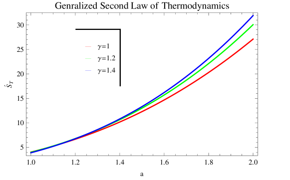
Figure 1: Plot of ${S^{\prime}}_{T}$ versus $a$ for Bekenstein entropy using $k=1,~{}\lambda=-1$ and $b=1$.

The graphical behavior of ${S^{\prime}}_{T}$ versus scale factor $a$ is shown in Figure 1. It can be observed that GSLT satisfy the condition ${S^{\prime}}_{T}\geq 0$ for chosen three values of $\gamma$ which leads to the validity of GSLT.

In order to discuss the thermodynamical equilibrium, we obtain the second order differential equation by using Eq.(20), as follows

$$S^{{}^{\prime\prime}}_{T} = \frac{3bk\gamma\sqrt{3}a^{-2-\frac{3\gamma(4k\lambda-1)}{(3k\lambda\gamma-1)}}}{2\big{(}\frac{bk(3k\lambda\gamma-1)a^{-\frac{3\gamma(4k\lambda-1)}{(3k\lambda\gamma-1)}}}{(4k\lambda-1)}\big{)}^{\frac{3}{2}}}\bigg{(}-\frac{9\sqrt{3}b\gamma^{2}(4k\lambda-1)^{2}a^{-\frac{3\gamma(4k\lambda-1)}{(3k\lambda\gamma-1)}}}{16(3k\lambda\gamma-1)^{2}\big{(}\frac{bk(3k\lambda\gamma-1)a^{-\frac{3\gamma(4k\lambda-1)}{(3k\lambda\gamma-1)}}}{(4k\lambda-1)}\big{)}^{\frac{3}{2}}}+3bk\gamma$$ (21)

$$\times \frac{\sqrt{3}a^{-\frac{3\gamma(4k\lambda-1)}{(3k\lambda\gamma-1)}}\big{(}1+\frac{2\gamma}{4\gamma-1}\big{)}}{8\big{(}\frac{bk(3k\lambda\gamma-1)a^{-\frac{3\gamma(4k\lambda-1)}{(3k\lambda\gamma-1)}}}{(4k\lambda-1)}\big{)}^{\frac{3}{2}}}\bigg{)}-\frac{\sqrt{3}}{a^{2}\sqrt{\frac{bk(3k\lambda\gamma-1)a^{-\frac{3\gamma(4k\lambda-1)}{(3k\lambda\gamma-1)}}}{(4k\lambda-1)}}}\bigg{(}-\frac{(4k\lambda-1)^{2}}{(3k\lambda\gamma-1)^{2}}$$

$$\times \bigg{(}\frac{9\sqrt{3}b\gamma^{2}a^{-\frac{3\gamma(4k\lambda-1)}{(3k\lambda\gamma-1)}}}{16\big{(}\frac{bk(3k\lambda\gamma-1)a^{-\frac{3\gamma(4k\lambda-1)}{(3k\lambda\gamma-1)}}}{(4k\lambda-1)}\big{)}^{\frac{3}{2}}}\bigg{)}+\frac{3bk\gamma\sqrt{3}a^{-\frac{3\gamma(4k\lambda-1)}{(3k\lambda\gamma-1)}}\big{(}1+\frac{2\gamma}{4\gamma-1}\big{)}}{8\big{(}\frac{bk(3k\lambda\gamma-1)a^{-\frac{3\gamma(4k\lambda-1)}{(3k\lambda\gamma-1)}}}{(4k\lambda-1)}\big{)}^{\frac{3}{2}}}\bigg{)}+\frac{\sqrt{3}}{a}$$

$$\times \frac{1}{\sqrt{\frac{bk(3k\lambda\gamma-1)a^{-\frac{3\gamma(4k\lambda-1)}{(3k\lambda\gamma-1)}}}{(4k\lambda-1)}}}\bigg{(}\frac{27b^{2}k^{2}\gamma^{2}a^{-1-\frac{6\gamma(4k\lambda-1)}{(3k\lambda\gamma-1)}}\big{(}1+\frac{2\gamma}{4\gamma-1}\big{)}}{16\big{(}\frac{bk(3k\lambda\gamma-1)a^{-\frac{3\gamma(4k\lambda-1)}{(3k\lambda\gamma-1)}}}{(4k\lambda-1)}\big{)}^{\frac{5}{2}}}-\frac{81b^{2}k\gamma^{3}\sqrt{3}}{32(3k\lambda\gamma-1)^{2}}$$

$$\times \frac{a^{-1-\frac{6\gamma(4k\lambda-1)}{(3k\lambda\gamma-1)}}(4k\lambda-1)^{2}}{\big{(}\frac{bk(3k\lambda\gamma-1)a^{-\frac{3\gamma(4k\lambda-1)}{(3k\lambda\gamma-1)}}}{(4k\lambda-1)}\big{)}^{\frac{5}{2}}}+\frac{27b\gamma^{3}(4k\lambda-1)^{3}\sqrt{3}a^{-1-\frac{3\gamma(4k\lambda-1)}{(3k\lambda\gamma-1)}}}{16(3k\lambda\gamma-1)^{3}\big{(}\frac{bk(3k\lambda\gamma-1)a^{-\frac{3\gamma(4k\lambda-1)}{(3k\lambda\gamma-1)}}}{(4k\lambda-1)}\big{)}^{\frac{3}{2}}}-9bk\gamma^{2}$$

$$\times \frac{\sqrt{3}(4k\lambda-1)a^{-1-\frac{3\gamma(4k\lambda-1)}{(3k\lambda\gamma-1)}}\big{(}1+\frac{2\gamma}{4\gamma-1}\big{)}}{8(3k\lambda\gamma-1)\big{(}\frac{bk(3k\lambda\gamma-1)a^{-\frac{3\gamma(4k\lambda-1)}{(3k\lambda\gamma-1)}}}{(4k\lambda-1)}\big{)}^{\frac{3}{2}}}\bigg{)}.$$

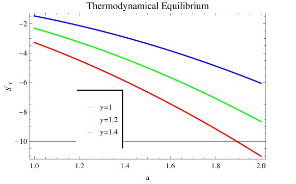
Figure 2: Plot of $S^{{}^{\prime\prime}}_{T}$ versus $a$ for Bekenstein entropy using $k=1,~{}\lambda=-1$, and $b=1$.

Figure 2 represents its plot against $a$. The trajectories of $S^{{}^{\prime\prime}}_{T}$ indicate the positive behavior for three values of $\gamma$. This leads to the validity of thermodynamical equilibrium for all values of $\gamma$.

IV Thermodynamical Analysis for Logarithmic Corrected Entropy

To study the expansion of entropy of the universe, we discuss the addition of entropy related to the horizon. Quantum gravity allows the logarithmic corrections in the presence of thermal equilibrium fluctuations and quantum fluctuations 7 -epjcn1 . Using the quantum gravity, one can get the corrected Wald entropy of horizons as epjcn1

$$S=S_{W}+\alpha\ln S_{W}+....,$$ (22)

where $\alpha$ is an unknown coefficient. The attempts for the Bekenstein-Hawking entropy ($S_{BH}$), as the Wald entropy in the Einstein theory wald , lead to 090 ; 0901 ; 0902

$$S=S_{BH}+\alpha\ln S_{BH}+\frac{\beta}{S_{BH}}+...$$ (23)

where $\beta$ is constant whose value is still under consideration (the same as $\alpha$). On one hand, Eq. (11) indicates that the difference between $S_{A}$, which is a proper candidate for the Wald entropy in the Rastall theory, and $S_{BH}$ is a constant coefficient ($1+\frac{2\gamma}{1+4\gamma}$). On the other hand, the same result as Eq. (23) is also obtainable by studying the effects of the thermal fluctuations on the horizon entropy 90 ; 9 , and indeed, these thermal-based approaches are not restricted to $S_{BH}$ 90 ; 9 . Therefore, we assume Eq. (23) is also valid for the Rastall theory, and write the logarithmic entropy corrected as

$$S_{A}=\frac{\tilde{A}}{4L^{2}_{p}}+\alpha\ln\frac{\tilde{A}}{4L^{2}_{p}}+\beta\frac{4L^{2}_{p}}{\tilde{A}},$$ (24)

where $L_{P}$ is the Planck’s length. The differential form of above equation is given by

$$dS_{A}=\frac{k\gamma ba^{-\frac{3\gamma(4k\lambda-1)}{(3k\lambda\gamma-1)}}}{2H^{2}}\bigg{(}\frac{(1+\frac{2\gamma}{1+4\gamma})}{4HL^{2}_{p}}+2\alpha H-\frac{16\beta H^{3}L^{2}_{p}}{(1+\frac{2\gamma}{1+4\gamma})}\bigg{)}dt,$$ (25)

which yields

$$T_{A}dS_{A}=\frac{2k\gamma ba^{-\frac{3\gamma(4k\lambda-1)}{(3k\lambda\gamma-1)}}}{H}\bigg{(}\frac{(1+\frac{2\gamma}{1+4\gamma})}{4HL^{2}_{p}}+2\alpha H-\frac{16\beta H^{3}L^{2}_{p}}{(1+\frac{2\gamma}{1+4\gamma})}\bigg{)}dt.$$ (26)

Using Eq.(15), we get

$$\Omega=\frac{2k\gamma ba^{-\frac{3\gamma(4k\lambda-1)}{(3k\lambda\gamma-1)}}}{H}\bigg{(}\frac{(1+\frac{2\gamma}{1+4\gamma})}{4HL^{2}_{p}}+2\alpha H-\frac{16\beta H^{3}L^{2}_{p}}{(1+\frac{2\gamma}{1+4\gamma})}\bigg{)}-\frac{\gamma ba^{-\frac{3\gamma(4k\lambda-1)}{(3k\lambda\gamma-1)}}}{2H^{2}}.$$ (27)

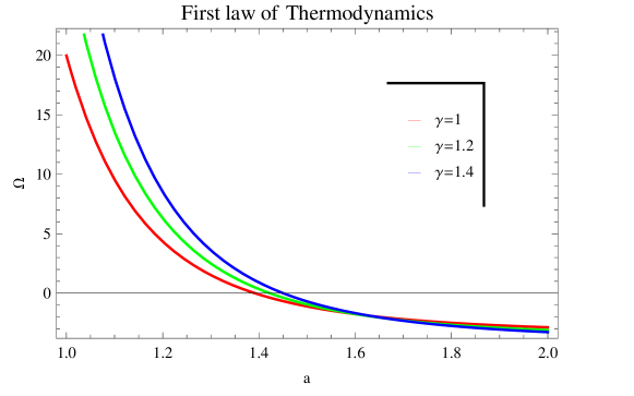
Figure 3: Plot of $\Omega$ versus $a$ for logarithmic corrected entropy using $k=1,~{}\lambda=-1,~{}\alpha=-1,~{}L_{p}=1,~{}\beta=1$ and $b=1$.

The plot of $\Omega$ versus $a$ for three values of $\gamma$ taking same values of constants as previous case is shown in Figure 3. It can be observed that first law of thermodynamics holds for some specific values of $a$ , i.e., for $\gamma=1$ at $a=1.39$, at $a=1.43$ for $\gamma=1.2$ and for $\gamma=1.4$ at $a=1.45$ represent the validity of first law of thermodynamics.

Moreover, we analyze the validity of GSLT and thermodynamical equilibrium which hold if $dS_{T}\geq 0$ and $d^{2}S_{T}<0$ satisfy respectively. From Eqs.(18) and (25), we get

$$\dot{S_{T}} = \frac{k\gamma ba^{-\frac{3\gamma(4k\lambda-1)}{(3k\lambda\gamma-1)}}}{2H^{2}}\bigg{(}\frac{(1+\frac{2\gamma}{1+4\gamma})}{4HL^{2}_{p}}+2\alpha H-\frac{16\beta H^{3}L^{2}_{p}}{(1+\frac{2\gamma}{1+4\gamma})}\bigg{)}+\frac{\gamma b}{8H^{3}}$$ (28)

$$\times a^{-\frac{3\gamma(4k\lambda-1)}{(3k\lambda\gamma-1)}}\bigg{(}\frac{(1-4k\lambda)}{(3k\lambda\gamma-1)}+\frac{k\gamma ba^{-\frac{3\gamma(4k\lambda-1)}{(3k\lambda\gamma-1)}}}{2H^{2}}\bigg{)}.$$

This equation leads to the following equation

$$\acute{S}_{T} = \frac{1}{aH}\bigg{(}\frac{k\gamma ba^{-\frac{3\gamma(4k\lambda-1)}{(3k\lambda\gamma-1)}}}{2H^{2}}\bigg{(}\frac{(1+\frac{2\gamma}{1+4\gamma})}{4HL^{2}_{p}}+2\alpha H-\frac{16\beta H^{3}L^{2}_{p}}{(1+\frac{2\gamma}{1+4\gamma})}\bigg{)}+\frac{\gamma b}{8H^{3}}$$ (29)

$$\times a^{-\frac{3\gamma(4k\lambda-1)}{(3k\lambda\gamma-1)}}\bigg{(}\frac{(1-4k\lambda)}{(3k\lambda\gamma-1)}+\frac{k\gamma ba^{-\frac{3\gamma(4k\lambda-1)}{(3k\lambda\gamma-1)}}}{2H^{2}}\bigg{)}\bigg{)}.$$

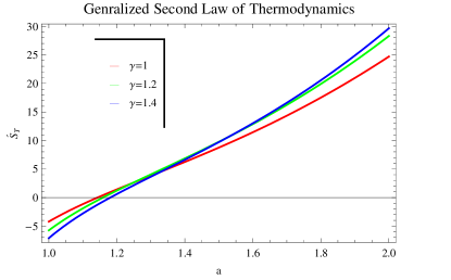
Figure 4: Plot of $\acute{S}_{T}$ versus $a$ for logarithmic corrected entropy using $k=1,~{}\lambda=-1,~{}\alpha=-1,~{}L_{p}=1,~{}\beta=1$ and $b=1$.

In case of logarithmic corrected entropy, we analyze the behavior of GSLT by plotting the graph of $\acute{S}_{T}$ versus scale factor as shown in Figure 4. The trajectories of GSLT meets the condition $\acute{S}_{T}\geq 0$ for all the three vales of $\gamma$ for specific ranges of $a$. For $1.26<a,~{}1.27<a$ and $1.28<a$ corresponding to $\gamma=1,~{}1.2$ and $1.4$ respectively indicates the positive behavior expressing the validity of GSLT.

In order to discuss the thermodynamical equilibrium, we again differentiate the above equation. It is given by

$$S^{{}^{\prime\prime}}_{T} = \frac{\sqrt{3}}{a\sqrt{\frac{bk(3k\lambda\gamma-1)a^{-\frac{3\gamma(4k\lambda-1)}{(3k\lambda\gamma-1)}}}{(4k\lambda-1)}}}\bigg{(}\frac{27b^{2}\gamma^{2}k\sqrt{3}a^{-\frac{3\gamma(4k\lambda-1)}{(3k\lambda\gamma-1)}}\big{(}\frac{3\gamma(4k\lambda-1)}{2(3k\lambda\gamma-1)}-\frac{4k\lambda-1}{3k\lambda\gamma-1}\big{)}}{16\big{(}\frac{bk(3k\lambda\gamma-1)a^{-\frac{3\gamma(4k\lambda-1)}{(3k\lambda\gamma-1)}}}{(4k\lambda-1)}\big{)}^{\frac{5}{2}}}$$ (30)

$$- \frac{9b\gamma^{2}\sqrt{3}(4k\lambda-1)a^{-1-\frac{3\gamma(4k\lambda-1)}{(3k\lambda\gamma-1)}}\big{(}\frac{3\gamma(4k\lambda-1)}{2(3k\lambda\gamma-1)}-\frac{4k\lambda-1}{3k\lambda\gamma-1}\big{)}}{8(3k\lambda\gamma-1)\big{(}\frac{bk(3k\lambda\gamma-1)a^{-\frac{3\gamma(4k\lambda-1)}{(3k\lambda\gamma-1)}}}{(4k\lambda-1)}\big{)}^{\frac{3}{2}}}+\frac{3\gamma(4k\lambda-1)}{2(3k\lambda\gamma-1)}$$

$$\times \bigg{(}\frac{3bk\gamma\sqrt{3}a^{-1-\frac{3\gamma(4k\lambda-1)}{(3k\lambda\gamma-1)}}(1+\frac{2\gamma}{1+4\gamma})}{8L^{2}_{p}\big{(}\frac{bk(3k\lambda\gamma-1)a^{-\frac{3\gamma(4k\lambda-1)}{(3k\lambda\gamma-1)}}}{(4k\lambda-1)}\big{)}^{\frac{3}{2}}}-\frac{bk\alpha\gamma\sqrt{3}a^{-1-\frac{3\gamma(4k\lambda-1)}{(3k\lambda\gamma-1)}}}{\sqrt{\frac{bk(3k\lambda\gamma-1)a^{-\frac{3\gamma(4k\lambda-1)}{(3k\lambda\gamma-1)}}}{(4k\lambda-1)}}}+8bkL^{2}_{p}\beta$$

$$\times \gamma a^{-1-\frac{3\gamma(4k\lambda-1)}{(3k\lambda\gamma-1)}}\sqrt{\frac{bk(3k\lambda\gamma-1)a^{-\frac{3\gamma(4k\lambda-1)}{(3k\lambda\gamma-1)}}}{(4k\lambda-1)}}\bigg{)}\bigg{)}+3bk\gamma\sqrt{3}a^{-2-\frac{3\gamma(4k\lambda-1)}{(3k\lambda\gamma-1)}}$$

$$\times \frac{1}{2\big{(}\frac{bk(3k\lambda\gamma-1)a^{-\frac{3\gamma(4k\lambda-1)}{(3k\lambda\gamma-1)}}}{(4k\lambda-1)}\big{)}^{\frac{3}{2}}}\bigg{(}\frac{3b\gamma\sqrt{3}a^{-\frac{3\gamma(4k\lambda-1)}{(3k\lambda\gamma-1)}}\big{(}\frac{3\gamma(4k\lambda-1)}{2(3k\lambda\gamma-1)}-\frac{4k\lambda-1}{3k\lambda\gamma-1}\big{)}}{8\big{(}\frac{bk(3k\lambda\gamma-1)a^{-\frac{3\gamma(4k\lambda-1)}{(3k\lambda\gamma-1)}}}{(4k\lambda-1)}\big{)}^{\frac{3}{2}}}$$

$$+ \frac{3\gamma(4k\lambda-1)}{2(3k\lambda\gamma-1)}\bigg{(}\frac{\sqrt{3}(1+\frac{2\gamma}{1+4\gamma})}{4L^{2}_{p}\sqrt{\frac{bk(3k\lambda\gamma-1)a^{-\frac{3\gamma(4k\lambda-1)}{(3k\lambda\gamma-1)}}}{(4k\lambda-1)}}}+\frac{2\alpha\sqrt{\frac{bk(3k\lambda\gamma-1)a^{-\frac{3\gamma(4k\lambda-1)}{(3k\lambda\gamma-1)}}}{(4k\lambda-1)}}}{\sqrt{3}}$$

$$- \frac{16L^{2}_{p}\beta\big{(}\frac{bk(3k\lambda\gamma-1)a^{-\frac{3\gamma(4k\lambda-1)}{(3k\lambda\gamma-1)}}}{(4k\lambda-1)}\big{)}^{\frac{3}{2}}}{3\sqrt{3}}\bigg{)}\bigg{)}-\frac{\sqrt{3}}{a^{2}\sqrt{\frac{bk(3k\lambda\gamma-1)a^{-\frac{3\gamma(4k\lambda-1)}{(3k\lambda\gamma-1)}}}{(4k\lambda-1)}}}$$

$$\times \bigg{(}\frac{3b\gamma a^{-\frac{3\gamma(4k\lambda-1)}{(3k\lambda\gamma-1)}}\big{(}\frac{3\gamma(4k\lambda-1)}{2(3k\lambda\gamma-1)}-\frac{4k\lambda-1}{3k\lambda\gamma-1}\big{)}}{8\big{(}\frac{bk(3k\lambda\gamma-1)a^{-\frac{3\gamma(4k\lambda-1)}{(3k\lambda\gamma-1)}}}{(4k\lambda-1)}\big{)}^{\frac{3}{2}}}+\frac{3\gamma(4k\lambda-1)}{2(3k\lambda\gamma-1)}\bigg{(}-\frac{16L^{2}_{p}\beta}{3\sqrt{3}}$$

$$\times \big{(}\frac{bk(3k\lambda\gamma-1)a^{-\frac{3\gamma(4k\lambda-1)}{(3k\lambda\gamma-1)}}}{(4k\lambda-1)}\big{)}^{\frac{3}{2}}+\frac{\sqrt{3}(1+\frac{2\gamma}{1+4\gamma})}{4L^{2}_{p}\sqrt{\frac{bk(3k\lambda\gamma-1)a^{-\frac{3\gamma(4k\lambda-1)}{(3k\lambda\gamma-1)}}}{(4k\lambda-1)}}}+\frac{2\alpha}{\sqrt{3}}$$

$$\times \sqrt{\frac{bk(3k\lambda\gamma-1)a^{-\frac{3\gamma(4k\lambda-1)}{(3k\lambda\gamma-1)}}}{(4k\lambda-1)}}\bigg{)}\bigg{)}.$$

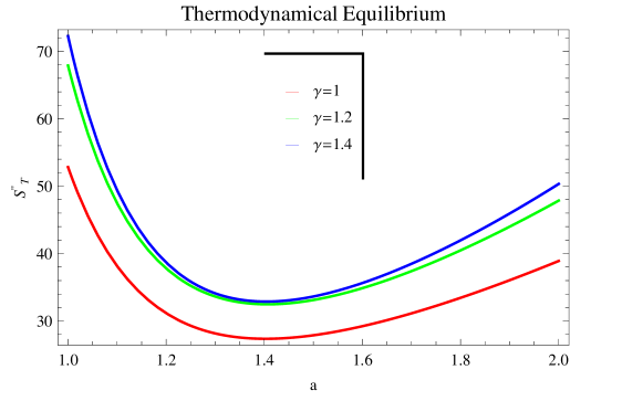
Figure 5: Plot of $S^{{}^{\prime\prime}}_{T}$ versus $a$ for logarithmic corrected entropy using $k=1,~{}\lambda=-1,~{}\alpha=-1,~{}L_{p}=1,~{}\beta=1$ and $b=1$.

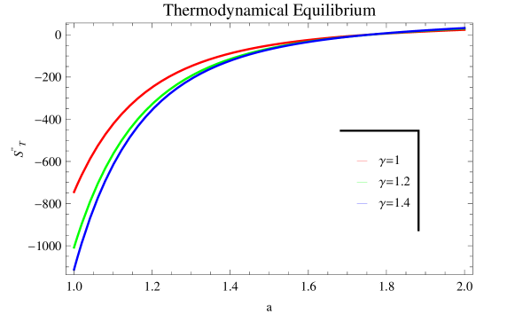
Figure 6: Plot of $S^{{}^{\prime\prime}}_{T}$ versus $a$ for logarithmic corrected entropy using $k=1,~{}\lambda=-1,~{}\alpha=-1,~{}L_{p}=1,~{}b=1$ and $\beta=-1$ in outer graph while $\beta=-20$ in inner graph.

The graphical behavior of $S^{{}^{\prime\prime}}_{T}$ versus $a$ is shown in Figure 5 for same constant values as mentioned above. We observe that all the trajectories express the positive behavior which represent non-equilibrium state of the solution. However, if we replace $\beta=-1$, we obtain the equilibrium states for $a\leq 1.2,~{}a\leq 1.225,~{}a\leq 1.24$ for logarithmic corrected entropy related to $\gamma=1,~{}1.2,~{}1.4$ respectively as shown in Figure 6 (outer graph). The inner plots in this Figure show the trajectories for replacing the value of $\beta=-20$ which indicate the negative behavior for more values of $a$. This leads to the result that we obtain the thermodynamical equilibrium as we decrease the value of $\beta$. However, first law of thermodynamics does not hold while GSLT satisfies for these negative values.

V Power-Law Corrected Entropy

The quantum corrections provided to the entropy-area relationship lead to the curvature corrections in the Einstein-Hilbert action and vice versa 14 -142 . As it has been shown in Ref. hooman , the linear entropy-area relation $(S\sim A)$ in the Rastall theory is the same as that of the Einstein theory ser . In addition, the entanglement of quantum fields between inside and outside of the horizon produces an entropy as $A^{m}$, where $m$ depends on the amount of mixing 15 . Thus, by adding this entropy to the horizon entropy 15 , one may get the power-law corrected entropy as 15

$$S_{\textmd{A}}=\frac{\tilde{A}}{4L^{2}_{p}}\big{(}1-F_{\alpha}\tilde{A}^{1-\frac{\alpha}{2}}\big{)},$$ (31)

where $F_{\alpha}=\frac{\alpha(4\pi)^{\frac{\alpha}{2}-1}}{(4-\alpha)r^{4-\alpha}_{c}},~{}\alpha$ is a dimensionless constant and $r_{c}$ represents the crossover scale. The differential of Eq.(31) is given by

$$dS_{A}=\frac{k\gamma ba^{-\frac{3\gamma(4k\lambda-1)}{(3k\lambda\gamma-1)}}}{2H^{2}}\bigg{(}\frac{(1+\frac{2\gamma}{1+4\gamma})}{4HL^{2}_{p}}-\frac{(1+\frac{2\gamma}{1+4\gamma})^{2-\frac{\alpha}{2}}F_{\alpha}}{4L^{2}_{p}}\big{(}2-\frac{\alpha}{2}\big{)}\big{(}\frac{1}{H}\big{)}^{3-\alpha}\bigg{)}dt,$$ (32)

which leads to

$$T_{A}dS_{A}=\frac{2bk\gamma a^{-\frac{3\gamma(4k\lambda-1)}{(3k\lambda\gamma-1)}}}{H}\bigg{(}\frac{(1+\frac{2\gamma}{1+4\gamma})}{4HL^{2}_{p}}-\frac{F_{\alpha}}{4L^{2}_{p}}\big{(}2-\frac{\alpha}{2}\big{)}\big{(}\frac{1}{H}\big{)}^{3-\alpha}\bigg{)}dt.$$ (33)

Combining Eqs.(13) and (31), we get

$$\Omega=\frac{2bk\gamma a^{-\frac{3\gamma(4k\lambda-1)}{(3k\lambda\gamma-1)}}}{H}\bigg{(}\frac{(1+\frac{2\gamma}{1+4\gamma})}{4HL^{2}_{p}}-\frac{(1+\frac{2\gamma}{1+4\gamma})^{2-\frac{\alpha}{2}}F_{\alpha}}{4L^{2}_{p}}\big{(}2-\frac{\alpha}{2}\big{)}\big{(}\frac{1}{H}\big{)}^{3-\alpha}\bigg{)}-\frac{\gamma ba^{-\frac{3\gamma(4k\lambda-1)}{(3k\lambda\gamma-1)}}}{2H^{2}}.$$ (34)

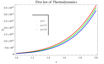
Figure 7: Plot of $\Omega$ versus $a$ for power law corrected entropy using $k=1,~{}\lambda=-1,~{}\alpha=1,~{}L_{p}=1,~{}r_{c}=\frac{1}{67}$ and $b=1$.

Figure 7 represents that the trajectories of $\Omega$ against $a$ with respect to three values of $\gamma$ approach to zero which indicates the validity of first law of thermodynamics.

To discuss the GSLT for power law corrected entropy at event horizon, we obtain the total entropy by using Eqs.(18) and (32) as

$$\dot{S_{T}} = \frac{\gamma ba^{-\frac{3\gamma(4k\lambda-1)}{(3k\lambda\gamma-1)}}}{8H^{3}}\bigg{(}\frac{(1-4k\lambda)}{(3k\lambda\gamma-1)}+\frac{k\gamma ba^{-\frac{3\gamma(4k\lambda-1)}{(3k\lambda\gamma-1)}}}{2H^{2}}\bigg{)}+\frac{k\gamma ba^{-\frac{3\gamma(4k\lambda-1)}{(3k\lambda\gamma-1)}}}{2H^{2}}$$ (35)

$$\times \bigg{(}\frac{(1+\frac{2\gamma}{1+4\gamma})}{4HL^{2}_{p}}-\frac{(1+\frac{2\gamma}{1+4\gamma})^{2-\frac{\alpha}{2}}F_{\alpha}}{4L^{2}_{p}}\big{(}2-\frac{\alpha}{2}\big{)}\big{(}\frac{1}{H}\big{)}^{3-\alpha}\bigg{)}.$$

The above equation reduces to

$$\acute{S}_{T} = \frac{1}{aH}\bigg{(}\frac{\gamma ba^{-\frac{3\gamma(4k\lambda-1)}{(3k\lambda\gamma-1)}}}{8H^{3}}\bigg{(}\frac{(1-4k\lambda)}{(3k\lambda\gamma-1)}+\frac{k\gamma ba^{-\frac{3\gamma(4k\lambda-1)}{(3k\lambda\gamma-1)}}}{2H^{2}}\bigg{)}$$ (36)

$$+ \frac{k\gamma ba^{-\frac{3\gamma(4k\lambda-1)}{(3k\lambda\gamma-1)}}}{2H^{2}}\big{(}\frac{(1+\frac{2\gamma}{1+4\gamma})}{4HL^{2}_{p}}-\frac{(1+\frac{2\gamma}{1+4\gamma})^{2-\frac{\alpha}{2}}F_{\alpha}}{4L^{2}_{p}}\big{(}2-\frac{\alpha}{2}\big{)}\big{(}\frac{1}{H}\big{)}^{3-\alpha}\big{)}\bigg{)}.$$

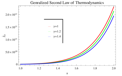
Figure 8: Plot of $\acute{S}_{T}$ versus $a$ for power law corrected entropy using $k=1,~{}\lambda=-1,~{}\alpha=-1,~{}L_{p}=1,~{}r_{c}=\frac{1}{67}$ and $b=1$.

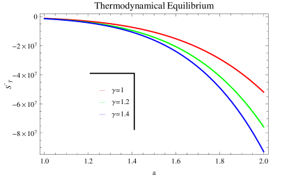
Figure 9: Plot of $S^{{}^{\prime\prime}}_{T}$ versus $a$ for power law corrected entropy using $k=1,~{}\lambda=-1,~{}\alpha=1,~{}L_{p}=1,~{}r_{c}=\frac{1}{67}$ and $b=1$.

The graphical behavior of $\acute{S}_{T}$ against $a$ is shown in Figure 8 for three values of $\gamma$. The trajectories follow the condition $\acute{S}_{T}\geq 0$ by expressing positive behavior, which leads to the validity of GSLT for all values $\gamma$. From Eq.(35), we find the second order differential equation as follows

$$S^{{}^{\prime\prime}}_{T} = \frac{27\gamma^{2}(4k\lambda-1)^{3}a^{-1+\frac{3\gamma(4k\lambda-1)}{(3k\lambda\gamma-1)}}\big{(}\frac{3\gamma(4k\lambda-1)}{2(3k\lambda\gamma-1)}-\frac{4k\lambda-1}{3k\lambda\gamma-1}\big{)}}{16bk^{2}(3k\lambda\gamma-1)^{3}}\bigg{(}3bk\gamma a^{-1-\frac{3\gamma(4k\lambda-1)}{(3k\lambda\gamma-1)}}$$ (37)

$$\times \frac{\sqrt{3}(1+\frac{2\gamma}{1+4\gamma})}{8L^{2}_{p}\big{(}\frac{bk(3k\lambda\gamma-1)a^{-\frac{3\gamma(4k\lambda-1)}{(3k\lambda\gamma-1)}}}{(4k\lambda-1)}\big{)}^{\frac{3}{2}}}+3^{1+\frac{3-\alpha}{2}}(\alpha-3)(2-\frac{\alpha}{2})a^{-1-\frac{3\gamma(4k\lambda-1)}{(3k\lambda\gamma-1)}}$$

$$\times \frac{\alpha bk\gamma F_{\alpha}(1+\frac{2\gamma}{1+4\gamma})^{2-\frac{\alpha}{2}}\big{(}\frac{bk(3k\lambda\gamma-1)a^{-\frac{3\gamma(4k\lambda-1)}{(3k\lambda\gamma-1)}}}{(4k\lambda-1)}\big{)}^{-1+\frac{\alpha-3}{2}}}{8L^{2}_{p}}\bigg{)}+27\gamma^{2}(4k\lambda-1)^{3}$$

$$\times \frac{a^{-2+\frac{3\gamma(4k\lambda-1)}{(3k\lambda\gamma-1)}}\big{(}\frac{3\gamma(4k\lambda-1)}{2(3k\lambda\gamma-1)}-\frac{4k\lambda-1}{3k\lambda\gamma-1}\big{)}\big{(}-1+\frac{3\gamma(4k\lambda-1)}{3k\lambda\gamma-1}\big{)}}{16bk^{2}(-1+3k\lambda\gamma)^{3}}\bigg{(}\frac{{1}}{\sqrt{\frac{bk(3k\lambda\gamma-1)a^{-\frac{3\gamma(4k\lambda-1)}{(3k\lambda\gamma-1)}}}{(4k\lambda-1)}}}$$

$$\times \frac{\sqrt{3}}{4L^{2}_{p}}-\frac{F_{\alpha}3^{\frac{3-\alpha}{2}}(2-\frac{\alpha}{2})\big{(}\frac{bk(3k\lambda\gamma-1)a^{-\frac{3\gamma(4k\lambda-1)}{(3k\lambda\gamma-1)}}}{(4k\lambda-1)}\big{)}^{\frac{\alpha-3}{2}}}{4L^{2}_{p}}\bigg{)}.$$

Figure 9 is showing the graph of $S^{{}^{\prime\prime}}_{T}$ versus scale factor for $\alpha=1$ respectively. The graph indicates the thermodynamical equilibrium as the plots are negative for all the values of $\gamma$.

VI The Renyi entropy

A novel sort of the Renyi entropy has been inspected in various cosmological and gravitational setups 17 ; 18 ; non20 . In which not exclusively is the logarithmic corrected entropy of the original, the Renyi entropy is utilized based on the fact that the Bekenstein Hawking entropy $S_{BH}$ is a Tsallis entropy $S_{A}$ 50 . One can obtain the Renyi entropy $S_{R}$ 18

$$S_{R}=\frac{\ln(1+\eta S_{A})}{\eta}.$$ (38)

The differential of this surface entropy is given by

$$dS_{R}=\frac{k\gamma ba^{-\frac{3\gamma(4k\lambda-1)}{(3k\lambda\gamma-1)}}}{2H}\big{(}\frac{(1+\frac{2\gamma}{4\gamma-1})}{\eta(1+\frac{2\gamma}{4\gamma-1})+8H^{2}}\big{)}dt,$$ (39)

which leads to

$$T_{A}dS_{R}=k\gamma ba^{-\frac{3\gamma(4k\lambda-1)}{(3k\lambda\gamma-1)}}\big{(}\frac{2(1+\frac{2\gamma}{4\gamma-1})}{\eta(1+\frac{2\gamma}{4\gamma-1})+8H^{2}}\big{)}dt.$$ (40)

Both of these equations take the form

$$\Omega=k\gamma ba^{-\frac{3\gamma(4k\lambda-1)}{(3k\lambda\gamma-1)}}\big{(}\frac{2(1+\frac{2\gamma}{4\gamma-1})}{\eta(1+\frac{2\gamma}{4\gamma-1})+8H^{2}}\big{)}-\frac{\gamma ba^{-\frac{3\gamma(4k\lambda-1)}{(3k\lambda\gamma-1)}}}{2H^{2}}.$$ (41)

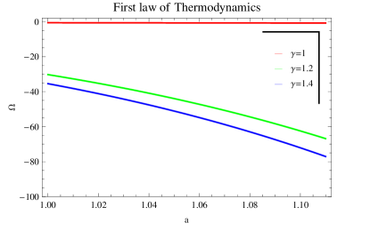
Figure 10: Plot of $\Omega$ versus $a$ for Renyi entropy using $k=1,~{}\lambda=-1,~{}\eta=1$ and $b=1$.

The numerical display of above differential equation for $\Omega$ against $a$ for different values of $\gamma$ is shown in Figure 10. The first law of thermodynamics does not hold for $\gamma-1.2,~{}1.4$ as all the corresponding trajectories fail to meet the condition $\Omega\rightarrow 0$. The trajectory for $\gamma=1$ represents the validity of first law of thermodynamics. Further, we analyze the validity of GSLT and thermodynamical equilibrium in the presence of Renyi entropy. Using Eqs.(18) and (39), we get

$$\dot{S_{T}} = \bigg{(}\frac{\gamma ba^{-\frac{3\gamma(4k\lambda-1)}{(3k\lambda\gamma-1)}}}{8H^{3}}\bigg{(}\frac{(1-4k\lambda)}{(3k\lambda\gamma-1)}+\frac{k\gamma ba^{-\frac{3\gamma(4k\lambda-1)}{(3k\lambda\gamma-1)}}}{2H^{2}}\bigg{)}$$ (42)

$$+ \frac{(1+\frac{2\gamma}{4\gamma-1})k\gamma ba^{-\frac{3\gamma(4k\lambda-1)}{(3k\lambda\gamma-1)}}}{2H}\big{(}\frac{2H}{\eta(1+\frac{2\gamma}{4\gamma-1})+8H^{2}}\big{)}\bigg{)},$$

$$\acute{S}_{T} = \frac{1}{aH}\bigg{(}\frac{\gamma ba^{-\frac{3\gamma(4k\lambda-1)}{(3k\lambda\gamma-1)}}}{8H^{3}}\bigg{(}\frac{(1-4k\lambda)}{(3k\lambda\gamma-1)}+\frac{k\gamma ba^{-\frac{3\gamma(4k\lambda-1)}{(3k\lambda\gamma-1)}}}{2H^{2}}\bigg{)}$$ (43)

$$+ \frac{(1+\frac{2\gamma}{4\gamma-1})k\gamma ba^{-\frac{3\gamma(4k\lambda-1)}{(3k\lambda\gamma-1)}}}{2H}\big{(}\frac{2H}{\eta(1+\frac{2\gamma}{4\gamma-1})+8H^{2}}\big{)}\bigg{)}\bigg{)}.$$

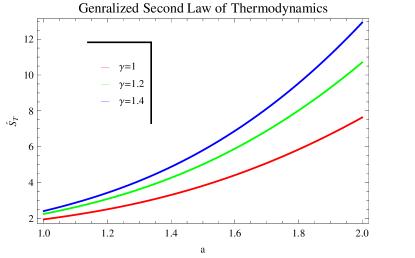
Figure 11: Plot of $\acute{S}_{T}$ versus $a$ for Renyi entropy using $k=1,~{}\lambda=-1,~{}\eta=1$ and $b=1$.

Figure 11 indicates the plot of $\acute{S}_{T}$ against scale factor $a$ for three values of $\gamma$. The trajectories in the plot are remain positive and obey the condition $\acute{S}_{T}\geq 0$ for all values of $\gamma$ which give the validity of GSLT. The second order differential equation takes the form

$$S^{{}^{\prime\prime}}_{T} = \frac{3\sqrt{3}bk\gamma a^{-2-\frac{3\gamma(4k\lambda-1)}{(3k\lambda\gamma-1)}}}{2\big{(}\frac{bk(3k\lambda\gamma-1)a^{-\frac{3\gamma(4k\lambda-1)}{(3k\lambda\gamma-1)}}}{(4k\lambda-1)}\big{)}^{\frac{3}{2}}}\bigg{(}\frac{3\sqrt{3}b\gamma a^{-\frac{3\gamma(4k\lambda-1)}{(3k\lambda\gamma-1)}}\big{(}\frac{3\gamma(4k\lambda-1)}{2(3k\lambda\gamma-1)}-\frac{4k\lambda-1}{3k\lambda\gamma-1}\big{)}}{8\big{(}\frac{bk(3k\lambda\gamma-1)a^{-\frac{3\gamma(4k\lambda-1)}{(3k\lambda\gamma-1)}}}{(4k\lambda-1)}\big{)}^{\frac{3}{2}}}$$ (44)

$$+ \frac{bk\gamma(1+\frac{2\gamma}{4\gamma-1})a^{-\frac{3\gamma(4k\lambda-1)}{(3k\lambda\gamma-1)}}}{\eta(1+\frac{2\gamma}{4\gamma-1})+\frac{8bk(3k\lambda\gamma-1)a^{-\frac{3\gamma(4k\lambda-1)}{(3k\lambda\gamma-1)}}}{3(4k\lambda-1)}}\bigg{)}-\frac{\sqrt{3}}{a^{2}\sqrt{\frac{bk(3k\lambda\gamma-1)a^{-\frac{3\gamma(4k\lambda-1)}{(3k\lambda\gamma-1)}}}{(4k\lambda-1)}}}$$

$$\times \bigg{(}\frac{3\sqrt{3}b\gamma a^{-\frac{3\gamma(4k\lambda-1)}{(3k\lambda\gamma-1)}}\big{(}\frac{3\gamma(4k\lambda-1)}{2(3k\lambda\gamma-1)}-\frac{4k\lambda-1}{3k\lambda\gamma-1}\big{)}}{8\big{(}\frac{bk(3k\lambda\gamma-1)a^{-\frac{3\gamma(4k\lambda-1)}{(3k\lambda\gamma-1)}}}{(4k\lambda-1)}\big{)}^{\frac{3}{2}}}+bk\gamma(1+\frac{2\gamma}{4\gamma-1})a^{-\frac{3\gamma(4k\lambda-1)}{(3k\lambda\gamma-1)}}$$

$$\times \frac{1}{\eta(1+\frac{2\gamma}{4\gamma-1})+\frac{8bk(3k\lambda\gamma-1)a^{-\frac{3\gamma(4k\lambda-1)}{(3k\lambda\gamma-1)}}}{3(4k\lambda-1)}}\bigg{)}+\frac{\sqrt{3}}{a\sqrt{\frac{bk(3k\lambda\gamma-1)a^{-\frac{3\gamma(4k\lambda-1)}{(3k\lambda\gamma-1)}}}{(4k\lambda-1)}}}$$

$$\times \bigg{(}\frac{27b^{2}\gamma^{2}k\sqrt{3}a^{-1-\frac{6\gamma(4k\lambda-1)}{(3k\lambda\gamma-1)}}\big{(}\frac{3\gamma(4k\lambda-1)}{2(3k\lambda\gamma-1)}-\frac{4k\lambda-1}{3k\lambda\gamma-1}\big{)}}{16\big{(}\frac{bk(3k\lambda\gamma-1)a^{-\frac{3\gamma(4k\lambda-1)}{(3k\lambda\gamma-1)}}}{(4k\lambda-1)}\big{)}^{\frac{5}{2}}}-9b\gamma^{2}\sqrt{3}a^{-\frac{3\gamma(4k\lambda-1)}{(3k\lambda\gamma-1)}}$$

$$\times \frac{(4k\lambda-1)\big{(}\frac{3\gamma(4k\lambda-1)}{2(3k\lambda\gamma-1)}-\frac{4k\lambda-1}{3k\lambda\gamma-1}\big{)}}{8(3k\lambda\gamma-1)\big{(}\frac{bk(3k\lambda\gamma-1)a^{-\frac{3\gamma(4k\lambda-1)}{(3k\lambda\gamma-1)}}}{(4k\lambda-1)}\big{)}^{\frac{3}{2}}}+\frac{8b^{2}k^{2}\gamma^{2}(1+\frac{2\gamma}{4\gamma-1})a^{-1-\frac{6\gamma(4k\lambda-1)}{(3k\lambda\gamma-1)}}}{\big{(}\eta(1+\frac{2\gamma}{4\gamma-1})+\frac{8bk(3k\lambda\gamma-1)a^{-\frac{3\gamma(4k\lambda-1)}{(3k\lambda\gamma-1)}}}{3(4k\lambda-1)}\big{)}^{2}}$$

$$- \frac{3bk\gamma^{2}(4k\lambda-1)(1+\frac{2\gamma}{4\gamma-1})a^{-1-\frac{3\gamma(4k\lambda-1)}{(3k\lambda\gamma-1)}}}{(3k\lambda\gamma-1)\big{(}\eta(1+\frac{2\gamma}{4\gamma-1})+\frac{8bk(3k\lambda\gamma-1)a^{-\frac{3\gamma(4k\lambda-1)}{(3k\lambda\gamma-1)}}}{3(4k\lambda-1)}\big{)}}\bigg{)}$$

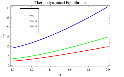
Figure 12: Plot of $S^{{}^{\prime\prime}}_{T}$ versus $a$ for Renyi entropy using $k=1,~{}\lambda=-1,~{}\eta=1$ and $b=1$.

The plot of $S^{{}^{\prime\prime}}_{T}$ versus $a$ for second order differential equation with apparent horizon as shown in Figure12. It is observed that $S^{{}^{\prime\prime}}_{T}\geq 0$ with all values of $\frac{2}{3}\leq\gamma\leq 2$ which leads to instability of thermodynamical equilibrium with $S^{{}^{\prime\prime}}_{T}<0$.

VII Conclusions

In the present paper, we have investigated the validity of first law of thermodynamics, GSLT and thermodynamical equilibrium for the flat FRW universe in Rastall theory of gravity. For this purpose, we have taken the EoS for perfect fluid by considering the different entropies including the modified Bekenstein entropy, the logarithmic corrected entropy, power law corrected entropy and the Renyi entropy. We have summarized our results as follows:

• For the modified Bekenstein entropy The plot of $\acute{S}_{T}$ versus scale factor parameter as shown in Figure 1 prove that GSLT is valid for all values of $\frac{2}{3}\leq\gamma\leq 2$. Further, we have observed the validity of thermodynamical equilibrium. Figure 2 indicates that thermodynamical equilibrium satisfies the condition $S^{{}^{\prime\prime}}_{T}<0$.

• For Logarithmic corrected entropy In the presence of logarithmic corrected entropy it can be seen that first law of thermodynamics is showing the validity for some specific points. These are for $\gamma=1$ at $a=1.39$, at $a=1.43$ for $\gamma=1.2$ and for $\gamma=1.4$ at $a=1.45$ represent the validity of first law of thermodynamics (Figure 3). The trajectories of GSLT meets the condition $\acute{S}_{T}\geq 0$ for all the three vales of $\gamma$ for specific ranges of $a$ which are $a>1.07,~{}a>1.08$ and $a>1.09$ corresponding to $\gamma=1,~{}1.2$ and $1.4$ respectively. (Figure 4). Further, the graphical behavior of $S^{{}^{\prime\prime}}_{T}$ against $a$ is shown in Figure 5 does not hold the thermodynamical equilibrium when $\beta$ is positive while Figure 6 provide the validity of thermodynamical equilibrium for all values of $\gamma$ with negative decreasing value of $\beta$.

• Power law Corrected Entropy In this entropy, we have analyzed that the first law of thermodynamics holds (Figure 7) as well as the GSLT is valid for all values $\gamma$ (Figure 8). From Figure (9), we have investigated that the thermodynamical equilibrium condition $S^{{}^{\prime\prime}}_{T}<0)$ satisfied with all values $a$ The trajectories of thermodynamical equilibrium are negative which lead to the instability of thermodynamical equilibrium.

• For the Renyi Entropy In this entropy, we have observed that the first law of thermodynamics does not hold for $\gamma-1.2,~{}1.4$ as all the corresponding trajectories fail to meet the condition $\Omega\rightarrow 0$. The trajectory for $\gamma=1$ represents the validity of first law of thermodynamics. (Figure 10). The graphical behavior of Figure 11 shows that all trajectories remains positive for all values of $\gamma$ which leads to the validity of GSLT. Moreover, thermodynamical equilibrium condition is not satisfied with all values of $\gamma$ (Figure 12).

References

(1) E. Poisson, A Relativist Toolkit (Cambridge University Press, UK,
2004).
(2) N. K. Glendenning, Special and General Relativity: With Applications
to White Dwarfs, Neutron Stars and Black Holes, (Springer, USA,
2007).
(3) M. Roos, Introduction to Cosmology (John Wiley and Sons, UK, 2003).
(4) P. Rastall, Phys. Rev. D 6, 3357 (1972).
(5) G. W. Gibbons and S. W. Hawking, Phys. Rev. D 15, 2738 (1977).
(8) N. D. Birrell, and P. C. W. Davies, Quantum Fieldsin Curved Space
(Cambridge University Press, Cambridge, 1982).
(9) C. E. M. Batista, M. H. Daouda, J. C. Fabris, O. F. Piattella, and
D. C. Rodrigues, Phys. Rev. D 85, 084008 (2012).
(10)
S. Nojiri and S. D. Odintsov,
Phys. Rept. 505, 59 (2011).
(11)
S. Nojiri and S. D. Odintsov,
eConf C 0602061 (2006) 06 [Int. J. Geom. Meth. Mod. Phys. 4, 115 (2007)].
(12)
S. Capozziello and V. Faraoni, Beyond Einstein Gravity
(Springer, Dordrecht, 2010).
(13)
S. Capozziello and M. De Laurentis,
Phys. Rept. 509, 167 (2011).
(14)
K. Bamba, S. Capozziello, S. Nojiri and S. D. Odintsov,
Astrophys. Space Sci. 342, 155 (2012).
(15)
A. Joyce, B. Jain, J. Khoury and M. Trodden,
Phys. Rept. 568, 1 (2015).
(16)
K. Koyama,
Rept. Prog. Phys. 79, 046902 (2016).
(17)
K. Bamba and S. D. Odintsov,
Symmetry 7, 1, 220 (2015).
(18)
S. Nojiri, S. D. Odintsov and V. K. Oikonomou,
Phys. Rept. 692, 1 (2017).
(19) T. Jacobson, Phys. Rev. Lett. 75, 1260 (1995).
(20) C. Eling, R. Guedens, and T. Jacobson, Phys. Rev. Lett. 96, 121301 (2006).
(21) M. Akbar, and R. G. Cai, Phys. Lett. B 648, 243 (2007).
(22) T. Padmanabhan, Phys. Rept. 406, 49 (2005).
(23) R. G. Cai, and S. P. Kim, JHEP 0502, 050 (2005).
(24) R. G. Cai, and L. M. Cao, Phys. Rev. D 75, 064008 (2007).
(25) S. W. Hawking, Phys. Rev. Lett. 26, 1344 (1971).
(26) T. Padmanabhan, Rep. Prog. Phys. 73, 046901 (2010).
(27) T. Padmanabhan, Class. Quantum Grav. 19, 5387 (2002).
(28) A. Sheykhi, B. Wang, R. G. Cai, Nucl. Phys. B 779, 1 (2007).
(29) A. Sheykhi, B. Wang, R. G. Cai, Phys. Rev. D 76, 023515 (2007).
(30) A. Sheykhi, M. H. Dehghani, R. Dehghani, Gen. Relativ. Gravit. 46, 1679 (2014).
(31) H. Moradpour, N. Sadeghnezhad, S. Ghaffari, and A. Jahan, AHEP. Article ID 9687976, (2017).
(32) H. Moradpour, Phys. Lett. B 757, 187 (2016), final version in arXiv:1601.04529.
(33) H. Moradpour, Ines. G. Salako, AHEP. Article ID 3492796, (2016).
(34) F. F. Yuan, P. Huang, arXiv:1607.04383.
(35) J. D. Bekenstein, Phys. Rev. D 7, 2333 (1973).
(36) R. Banerjee, and S. K. Modak, JHEP 073, 0911 (2009).
(37) H. Wei, Commun. Theor. Phys. 52, 743 (2009).
(38) S. Banerjee, R. K. Gupta, and A. Sen, JHEP 147,
1103 (2011).
(39) A. Sheykhi, and M. Jamil, Gen. Relativ. Gravit. 43, 2661 (2011).
(40)
K. Bamba, M. Jamil, D. Momeni and R. Myrzakulov,
Int. J. Mod. Phys. D 21, 1250065 (2012).
(41) K. Karami, S. Ghaffari, and M. M. Soltanzadeh, Class. Quantum Grav.
27, 205021 (2010).
(42) M. R. Setare, JCAP 01, 023 (2007).
(43) A. Sheykhi, Class. Quantum Grav. 27, 025007
(2010).
(44) M. Mazumder, and S. Chakraborty, Gen. Relativ. Gravit. 42,
813 (2010).
(45) M. Jamil, E. N. Saridakis, and M. R. Setare, Phys. Rev. D
81, 023007 (2010).
(46) K. Karami, et al., JHEP150, 1108 (2011).
(47) K. Karami, et al, Eur. Phys. Lett.93, 29002 (2011).
(48)
K. Bamba and C. Q. Geng,
Phys. Lett. B 679, 282 (2009).
(49)
K. Bamba, C. Q. Geng and S. Tsujikawa,
Phys. Lett. B 688, 101 (2010).
(50)
K. Bamba, C. Q. Geng, S. Nojiri and S. D. Odintsov,
EPL 89, 50003 (2010).
(51)
K. Bamba and C. Q. Geng,
JCAP 1006, 014 (2010).
(52)
K. Bamba and C. Q. Geng,
JCAP 1111, 008 (2011).
(53)
K. Bamba, R. Myrzakulov, S. Nojiri and S. D. Odintsov,
Phys. Rev. D 85, 104036 (2012).
(54)
K. Bamba, M. Jamil, D. Momeni and R. Myrzakulov,
Astrophys. Space Sci. 344, 259 (2013).
(55)
K. Bamba,
Int. J. Geom. Meth. Mod. Phys. 13, 1630007 (2016).
(56) L. L. Smalley, Il Nuovo Cimento B, 80, 1, 42 (1984)
(57) R. V. dos Santos, J. A. C. Nogales, arXiv:1701.08203v1.
(58) V. Dzhunushaliev and H. Quevedo, Grav. Cosm. 23, 280 (2017).
(59) H. Moradpour, I. Licata, C. Corda, Ines G. Salako, arXiv:1802.00738v1.
(60) L. L. Smalley, J. Phys. A: Math. Gen. 16, 2179 (1983).
(61) F. Darabi, H. Moradpour, I. Licata, Y. Heydarzade, C. Corda, EPJC 78, 25 (2018).
(62) H. Moradpour, A. Bonilla, E. M. C. Abreu, J. A. Neto, Phys. Rev. D 96, 123504 (2017).
(63) Mahamadou Daouda, J. C. Fabris, A. M. Oliveira, F. Smirnov, H. E. S. Velten, arXiv:1802.01413v1.
(64) M. Roos, Introduction to Cosmology (John Wiley and Sons, UK, 2003).
(65) M. Capone, V. F. Cardone, and M. L. Ruggiero, Journal of Physics:
Conference Series, D222, 012012 (2010).
(66) L. L. Smalley, and N. Cimento B 80(1), 42 (1984).
(67) R. Bousso, Phys. Rev. D 71, 064024 (2005).
(68) K. A. Miessner, Class. Quantum Grav. 21, 5245 (2004).
(69) A. Ghosh, and P. Mitra, Phys. Rev. D 71, 027502 (2004).
(70) R. M. Wald, Phys. Rev. D 48, 3427 (1993).
(71) R. K. Kaul, P. Majumdar, Phys. Rev. Lett. 84, 5255 (2000).
(72) S. Carlip, Class. Quant. Grav. 17, 4175 (2000).
(73) K. Nouicer, Phys. Lett. B 646, 63 (2007).
(74) S. Das, P. Majumdar, R. K. Bhaduri, Class. Quant. Grav.19, 2355 (2002).
(75) A. Chatterjee, and P. Majumder, Phys. Rev. Lett. 92, 141301 (2004).
(76) R. Banerjee, and S. K. Modak, JHEP 0905, 063 (2009).
(77) S. K. Modak, Phys. Lett. B 671, 167 (2009).
(78) M. Jamil, and M. U. Farooq, JCAP 03, 001 (2010).
(79) H. M. Sadjadi, and M. Jamil, Europhys. Lett. 92, 69001 (2010).
(80) S. Mahapatra, Eur. Phys. J. C 78, 23 (2018).
(81) R. Banerjee, and S. K. Modak, JHEP 05, 063 (2009).
(82) S. K. Modak, Phys. Lett. B 671, 167 (2009).
(83) R. Banerjee, S. Gangopadhyay, and S. K. Modak, Phys. Lett. B
686, 181 (2010).
(84) M. Srednicki, Phys. Rev. Lett. 71, 666 (1993).
(85) S. Das, S. Shankaranarayanan, P. Sur, Phys. Rev. D 77, 064013 (2008).
(86) B. Pourhassan, S. Upadhyay, and H. Farahani,
http://arxiv.org/abs/1701.08650.
(87) T. S. Biro, and V. G. Czinner, Phys. Lett. B 726, 861 (2013).
(88) V. G. Czinner, and H. Iguchi, Phys. Lett. B 752, 306 (2016).
(89)
M. Visser,
Phys. Lett. B 782, 83 (2018)
doi:10.1016/j.physletb.2018.05.028
[arXiv:1711.11500 [gr-qc]].
(90)
F. Darabi, H. Moradpour, I. Licata, Y. Heydarzade and C. Corda,
Eur. Phys. J. C 78, 25 (2018)
doi:10.1140/epjc/s10052-017-5502-5
[arXiv:1712.09307 [gr-qc]].
(91) H. Moradpour, I. G. Salako, Adv. High Ener. Phys. 2016, 3492796 (2016).
(92) R. G. Cai, L. M. Cao, Y. P. Hu, N. Ohta, Phys. Rev. D 80, 104016 (2009);
A. Paranjape, S. Sarkar, T.
Padmanabhan, Phys. Rev. D 74, 104015 (2006).
(93) D. Das, S. Dutta, S. Chakraborty, Eur. Phys. J. C 78, 810 (2018).
(94) F. F. Yuan, P. Huang, Class. Quantum Gravity 34, 077001 (2017).
(95) R. G. Cai, L. M. Cao, Y. P. Hu, Class. Quantum. Grav. 26, 155018 (2009).