Gapless odd-frequency superconductivity induced by the Sachdev-Ye-Kitaev model

Abstract

We show that a single fermion quantum dot acquires odd-frequency Gor’kov anomalous averages in proximity to strongly-correlated Majorana zero-modes, described by the Sachdev-Ye-Kitaev (SYK) model. Despite the presence of finite anomalous pairing, superconducting gap vanishes for the intermediate coupling strength between the quantum dot and Majoranas. The increase of the coupling leads to smooth suppression of the original quasiparticles. This effect might be used as a characterization tool for recently proposed tabletop realizations of the SYK model.

Introduction — The Sachdev-Ye-Kitaev (SYK) model SY ; Kitaev describes $N$ fermionic zero-modes with randomized infinite-range interaction. It comprises several important properties: (i) the SYK model possesses an exact large $N$ solution in the infrared lacking quasiparticles; (ii) it saturates Kitaev ; Maldacena1 the upper bound on quantum chaos Maldacena2 , which is also the case for holographic duals of black hole horizons Hartnoll . A possibility to study these intriguing properties in physical observables inspired a few proposals of realizing the SYK model in a solid-state platform Pikulin ; Alicea ; Pikulin2 .

The SYK model with Majorana (real) zero-modes is claimed to be a low-energy theory of the Fu-Kane superconductor FK in a magnetic field with a disordered openingPikulin , whereas Ref. Alicea, suggests to use $N$ Majorana nanowires DasSarma coupled through a disordered quantum dot. The graphene flake device proposed in Ref. Pikulin2, realizes the SYK model with the conventional (complex) fermionic zero-modes (cSYK model)Sachdev_BH . As for the latter one, the signatures of non-Fermi liquid/non-quasiparticle/quantum critical behavior Sachdev ; Hartnoll of the cSYK model have been recently studied in Refs. dIdV_SYK, ; Franz, ; Zeros, . The one dimensional extensions of the cSYK model to the coupled clusters uncover the Lyapunov time $|$the characteristic timescale of quantum chaos$|$ in thermal diffusion Sachdev_1D and demonstrate linear in temperature resistivity of strange metals Balents .

In this paper, we modify the SYK model with Majoranas via coupling it to a single-state non-interacting quantum dot. As we add only a single fermion, this model stays far away from the non-Fermi liquid/Fermi liquid transition Altman and it is still exactly solvable in the large $N$ limit. We demonstrate that the effective theory for the fermion in the quantum dot gains the anomalous pairing terms, that make the quantum dot superconducting. Despite the induced superconductivity, the density of states in the quantum dot has no excitation gap. It has been a while since the phenomenon of gapless superconductivity was found in the superconductors with magnetic impurities, where for a specific range of concentration of those, a part of electrons does not participate in the condensation process Abrikosov ; Woolf . The anomalous components of the Gor’kov Green’s function Gorkov ; AS of the quantum dot are calculated exactly in the large $N$ limit and are odd functions of frequency Berezinskii ; Balatsky . Odd-frequency pairing is known to be induced by proximity to an unconventional superconductor Balatsky ; Lutchyn1 ; Tanaka ; Tanaka_review . Below we obtain induced odd-frequency gapless superconductivity in zero dimensions as a consequence of the proximity to a system described by the SYK modelPikulin ; Alicea . We suggest to use this effect as a way to detect the SYK-like effective behavior in a solid-state system.

The model — Let’s consider the Sachdev-Ye-Kitaev model Kitaev ; Maldacena1 randomly coupled to a single state quantum dot Kouwenhoven with the frequency $\Omega_{d}$. The Hamiltonian of the system reads:

$$H\!\!=\!\Omega_{d}d^{\dagger}d\!+\!\!\sum_{i=1}^{N}\lambda_{i}\gamma_{i}\left(d^{\dagger}\!\!-\!d\right)\!+\!\frac{1}{4!}\!\!\sum_{i,j,k,l=1}^{N}\!\!J_{ijkl}\gamma_{i}\gamma_{j}\gamma_{k}\gamma_{l}\,,$$ (1)

where the couplings $J_{ijkl}$ and $\lambda_{i}$ are independently distributed as a Gaussian with zero mean $\overline{J_{ijkl}}=0=\overline{\lambda_{i}}$ and finite variance $\overline{J_{ijkl}^{2}}=3!J^{2}/N^{3}$,   $\overline{\lambda_{i}^{2}}=\lambda^{2}/N$. The tunneling term in the Hamiltonian (1) is similar to one, that appears for tunneling into Majorana nanowires Majorana_review ; Fisher ; Lutchyn3 ; Lutchyn1 ; Lutchyn2 .

Once the disorder averaging is done, we decouple the interactions by introducing four pairs of the non-local fields in the Euclidean action as a resolution of unityKitaev ; Maldacena1 :

$$1 {}=\!\!\int\!\!\mathcal{D}\Sigma_{\gamma}\mathcal{D}G_{\gamma}\mathrm{e}^{\int\!\!d\tau d\tau^{\prime}\frac{\Sigma_{\gamma}(\tau,\tau^{\prime})}{2}\!\left(\!N\!G_{\gamma}(\tau^{\prime},\tau)-\sum_{i}\!\!\gamma_{i}(\tau)\gamma_{i}(\tau^{\prime})\!\right)},$$ (2)

$$1 {}=\!\!\int\!\!\mathcal{D}\Sigma_{d}\mathcal{D}G_{d}\mathrm{e}^{\int\!\!d\tau d\tau^{\prime}\Sigma_{d}(\tau,\tau^{\prime})\left(\!G_{d}(\tau^{\prime},\tau)-\bar{d}(\tau)d(\tau^{\prime})\!\right)},$$ (3)

$$1 {}=\!\!\int\!\!\mathcal{D}\Xi_{d}\mathcal{D}F_{d}\mathrm{e}^{\int\!\!d\tau d\tau^{\prime}\Xi_{d}(\tau,\tau^{\prime})\left(\!F_{d}(\tau^{\prime},\tau)-d(\tau)d(\tau^{\prime})\!\right)},$$ (4)

$$1 {}=\!\!\int\!\!\mathcal{D}\bar{\Xi}_{d}\mathcal{D}\bar{F}_{d}\mathrm{e}^{\int\!\!d\tau d\tau^{\prime}\bar{\Xi}_{d}(\tau,\tau^{\prime})\left(\!\bar{F}_{d}(\tau^{\prime},\tau)-\bar{d}(\tau)\bar{d}(\tau^{\prime})\!\right)}.$$ (5)

A variation of the effective action, which is given in Appendix A, with respect to $G_{\gamma},G_{d},F_{d},\bar{F}_{d}$ and $\Sigma_{\gamma},\Sigma_{d},\Xi_{d},\bar{\Xi}_{d}$ produces self-consistent Schwinger-Dyson equations AS , that relate those fields to the Green’s functions and self-energies of Majorana fermions and the fermion in the quantum dot:

$$\Sigma_{d}(\tau)= {}\lambda^{2}G_{\gamma}(\tau),$$ (6)

$$\Xi_{d}(\tau)= {}-\frac{\lambda^{2}}{2}G_{\gamma}(\tau),\;\;\;\bar{\Xi}_{d}(\tau)=-\frac{\lambda^{2}}{2}G_{\gamma}(\tau),$$ (7)

$$\Sigma_{\gamma}(\tau)= {}J^{2}G_{\gamma}(\tau)^{3}+\!\frac{2\lambda^{2}}{N}\!\bigg{(}\!G_{d}(\tau)-\!\frac{F(\tau)}{2}\!-\!\frac{\bar{F}(\tau)}{2}\bigg{)},$$ (8)

$$G_{\gamma}(\mathrm{i}\omega_{n})= {}\bigg{(}\mathrm{i}\omega_{n}-\Sigma_{\gamma}(\mathrm{i}\omega_{n})\bigg{)}^{-1}.$$ (9)

The Green’s function of Majorana fermions is $G_{\gamma}(\tau)=-N^{-1}\sum_{i}\left\langle\mathcal{T}_{\tau}\,\gamma_{i}(\tau)\gamma_{i}(0)\right\rangle$ and $G_{d}(\tau)=-\left\langle\mathcal{T}_{\tau}\,d(\tau)\bar{d}(0)\right\rangle$, $F_{d}(\tau)=-\left\langle\mathcal{T}_{\tau}\,d(\tau)d(0)\right\rangle$, $\bar{F}_{d}(\tau)=-\left\langle\mathcal{T}_{\tau}\,\bar{d}(\tau)\bar{d}(0)\right\rangle$ are normal and anomalous Green’s functions of the quantum dot variables.

We are focused on the large $N$, long time limit $1\ll J\tau\ll N$, where the conformal symmetry of the SYK model emerges Kitaev ; Maldacena1 . In this regime, the backreaction of the quantum dot on the self-energy of Majorana fermions (8) is suppressed as $1/N$. The bare frequency in the equation (9) can also be omitted at low frequencies. Thus, equations (8, 9) become $\Sigma_{\gamma}(\tau)=J^{2}G_{\gamma}(\tau)^{3}$ and $G_{\gamma}(\mathrm{i}\omega_{n})=-\Sigma_{\gamma}(\mathrm{i}\omega_{n})^{-1}$, which are the same as in the case of the isolated SYK model. These equations have a known zero temperature solution Kitaev ; Maldacena1 $G_{\gamma}(\mathrm{i}\omega_{n})=-\mathrm{i}\pi^{1/4}\mathrm{sgn}(\omega_{n})\left(J|\omega_{n}|\right)^{-1/2}$, which contributes to the self-energies (6, 7) of the quantum dot. The Green’s function of Majorana zero-modes has no pole structure, which manifests the absence of quasiparticles. Moreover, it behaves as a power-law of frequency, which is the case of quantum criticality Sachdev and emergence of the conformal symmetry in the SYK case Kitaev ; Maldacena1 .

SYK proximity effect — The effective action for the fermion in the quantum dot acquires anomalous terms

$$S_{\rm eff}=-\frac{1}{2}\sum_{n=-\infty}^{+\infty}\begin{pmatrix}\bar{d}_{n}&d_{-n}\end{pmatrix}\mathcal{G}(\mathrm{i}\omega_{n})^{-1}\begin{pmatrix}d_{n}\\ \bar{d}_{-n}\end{pmatrix},$$ (10)

where the Gor’kov Green’s function Gorkov ; AS

$$\mathcal{G}(\mathrm{i}\omega_{n}\!)^{-1}\!=\!\!\begin{pmatrix}\mathrm{i}\omega_{n}\!\!-\!\Omega_{d}\!-\!\lambda^{2}G_{\gamma}(\mathrm{i}\omega_{n}\!)&\lambda^{2}G_{\gamma}(\mathrm{i}\omega_{n}\!)\\ \lambda^{2}G_{\gamma}(\mathrm{i}\omega_{n}\!)&\mathrm{i}\omega_{n}\!\!+\!\Omega_{d}\!-\!\lambda^{2}G_{\gamma}(\mathrm{i}\omega_{n}\!)\end{pmatrix}\!$$ (11)

is found self-consistently in a one loop expansion AS . Due to negligibility of the last term in Majoranas self-energy (8) mentioned above, the one loop approximation turns out to be exact in the large $N$ limit. A detailed derivation of the formula (11) is presented in Appendix A.

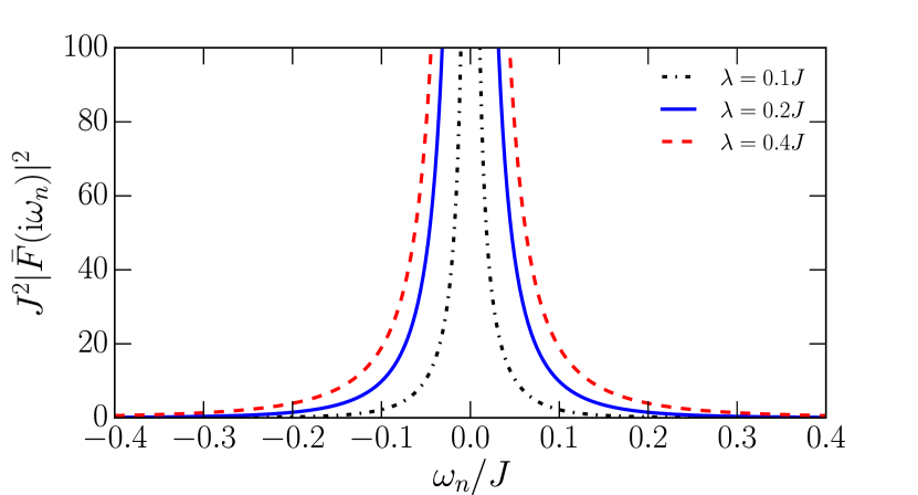
Figure 1: Absolute value of the anomalous averages as a function of Matsubara frequency. The frequency of the quantum dot is $\Omega_{d}=0.1J$.

Appearance of the anomalous pairing terms $\bar{d}(\tau)G_{\gamma}(\tau-\tau^{\prime})\bar{d}(\tau^{\prime})$ in the effective action (10) does not require any additional quantum numbers, because those are “glued” by the non-locality in the imaginary time that originates from the SYK saddle-point solution. The anomalous Green’s function which follows from (11) is odd in frequency Berezinskii ; Balatsky :

$$\bar{F}(\mathrm{i}\omega_{n})= {}-\frac{\lambda^{2}G_{\gamma}(\mathrm{i}\omega_{n})}{\mathrm{i}\omega_{n}\left(\mathrm{i}\omega_{n}-2\lambda^{2}G_{\gamma}(\mathrm{i}\omega_{n})\right)-\Omega_{d}^{2}}=$$

$$= {}-\bar{F}(-\mathrm{i}\omega_{n}).$$ (12)

This result (12) is well aligned with previously found proximity effect by Majorana zero modes Lutchyn1 ; Lutchyn2 and odd-frequency correlations found in interacting Majorana fermions Balatsky2 . Superconducting pairing grows smoothly while the coupling increases as it is shown in FIG. 1.

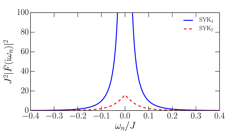
Figure 2: Anomalous averages in the quantum dot coupled to the SYK/SYK₂ model. The frequency of the dot is $\Omega_{d}=0.1J$ and the coupling strength is $\lambda=0.2J$.

It is worthwhile to compare our setting (1) to the case when the SYK quantum dot is replaced by a disordered Fermi liquid. The latter can be described by the SYK₂ model: $H_{{\rm SYK}_{2}}=\mathrm{i}\sum_{ij}J_{ij}\gamma_{i}\gamma_{j}$. In the long time limit, the Green’s function of the SYK₂ model is $G_{{\rm SYK}_{2}}(\mathrm{i}\omega_{n})=-\mathrm{i}\,\mathrm{sgn}(\omega_{n})/J$ Pikulin , which is substituted to the result for the anomalous component of the Gor’kov function (12). As we show in FIG. 2, the amount of the SYK induced superconductivity is sufficiently higher then in the case of the SYK₂ model.

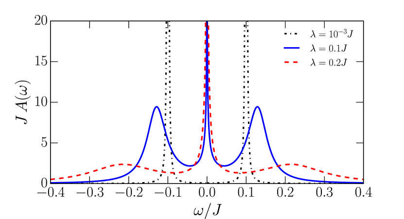
Figure 3: Density of states in the quantum dot at zero temperature as a function of frequency. $\Omega_{d}=0.1J$ and $\delta=10^{-3}J$.

In the large $N$ limit, the spectral function of the quantum dot is

$$A(\omega)= {}-\frac{1}{\pi}\mathrm{Im}\,\mathrm{tr}\mathcal{G}\left(\mathrm{i}\omega_{n}\to\omega+\mathrm{i}\delta\right)=$$

$$= {}-\frac{2}{\pi}\,\frac{\lambda^{2}\left(\omega^{2}+\Omega_{d}^{2}\right)\mathrm{Im}G^{R}_{\gamma}(\omega)}{\left|\omega\left(\omega-2\lambda^{2}G^{R}_{\gamma}(\omega)\right)-\Omega_{d}^{2}\right|^{2}}\,,$$ (13)

where $\delta=0^{+}$ and $G_{\gamma}^{R}(\omega)=-\mathrm{i}\pi^{1/4}\mathrm{e}^{\mathrm{i}\pi\mathrm{sgn}(\omega)/4}\left(J|\omega|\right)^{-1/2}$. The broadening $\delta=0^{+}$ of the fermion in the quantum dot is neglected once the imaginary part of the SYK Green’s function is finite: $\lambda^{2}\mathrm{Im}G^{R}_{\gamma}(\omega)\gg\delta=0^{+}$.

In absence of coupling between the single-state quantum dot and the SYK model ($\lambda=0$), there is no particle-hole mixing. Superconducting pairing (FIG. 1) appears in the regime of intermediate coupling. The absence of the gap in the presence of the anomalous pairing reveals gapless superconductivity Abrikosov ; Woolf in zero dimensions, which can be probed by Andreev reflection Andreev in the tunneling experiment. The wide broadening of the peaks in FIG. 3 is due to the binding of the fermionic quantum dot with the SYK quantum critical continuum Zeros . Increasing of coupling strength $\lambda$ results in grows of the anomalous pairing (12) and suppression of the initial quasiparticle peaks. In strong coupling the system shows divergent behavior at $\omega=0$. However, the divergence point might be addressed beyond the conformal limit Bagrets $\omega\lesssim J/\left(N\log N\right)$. This changes the scaling of the SYK Green’s function from $1/\sqrt{\omega}$ to $N\!\log N\sqrt{\omega}$ in the infrared.

In FIG. 4 we show, that the behavior of the spectral function of the quantum dot coupled to the SYK model is qualitatively different from the SYK₂ case. The SYK₂ model, mentioned above, describes disordered Fermi liquid and has a constant density of states $\propto 1/J$ in the long time limit.

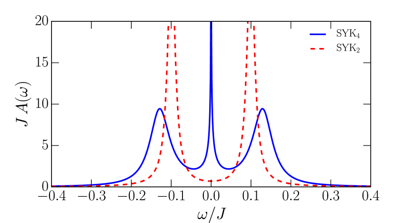
Figure 4: Density of states in the quantum dot coupled to the SYK/SYK₂ model at zero temperature. The coupling strength is $\lambda=0.1J$ and the frequency of the single state is $\Omega_{d}=0.1J$.

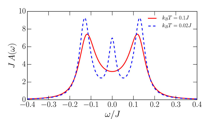
Figure 5: Density of states in the quantum dot at finite temperature as a function of frequency. The parameters are $\lambda/J=0.1=\Omega_{d}/J$.

At finite temperature the saddle-point solution of the SYK model is given by Sachdev_BH :

$$G^{R}_{\gamma}(\omega)=-\mathrm{i}\pi^{1/4}\sqrt{\frac{\beta}{2\pi J}}\,\frac{\Gamma\left(\frac{1}{4}-\mathrm{i}\frac{\beta\omega}{2\pi}\right)}{\Gamma\left(\frac{3}{4}-\mathrm{i}\frac{\beta\omega}{2\pi}\right)},$$ (14)

where $\beta=1/T$ is inverse temperature and $\Gamma(x)$ is the Gamma function. We substitute the finite temperature SYK Green’s function (14) in the spectral function of $d$ fermion (13). FIG. 5 demonstrates that the divergence around $\omega\sim 0$ in the quantum dot density of states is regularized at finite temperature.

Conclusion — In this paper, we have shown that a single-state spinless quantum dot becomes superconducting in proximity to a structure whose low-energy behavior can be captured by the Sachdev-Ye-Kitaev model. Anomalous averages are found exactly in the large $N$ limit and turn out to be odd functions of frequency. Appearance of non-zero superconducting pairing does not require any additional quantum numbers like spin, because it originates from non-locality of the SYK saddle-point solution. Induced superconductivity strikes in the intermediate coupling between the quantum dot and the SYK model. At stronger coupling, the quasiparticle peaks are smeared out on the background of the SYK quantum critical continuum. We propose to use the peculiar property of the induced gapless superconductivity in zero dimensions to characterize the solid-state systems, that can be described by the SYK model as an effective theory in a certain limit.

Acknowledgements — N. G. has benefited from discussions with Carlo Beenakker, Koenraad Schalm, Jakub Tworzydło, Fabian Hassler, İnanç Adagideli, Sergei Mukhin, Alexander Krikun, Jimmy Hutasoit, Michał Pacholski, Andrei Pavlov, and Yaroslav Herasymenko. This research was supported by the Netherlands Organization for Scientific Research (NWO/OCW) and by an ERC Synergy Grant.

Appendix A Self-consistent derivation of the Gor’kov Green’s function for the quantum dot variables

The Euclidean action that corresponds to the Hamiltonian (1) after disorder averaging is

$$S= {}\int_{0}^{\beta}d\tau\left[\bar{d}\left(\partial_{\tau}+\Omega_{d}\right)d+\frac{1}{2}\sum_{i=1}^{N}\gamma_{i}\partial_{\tau}\gamma_{i}\right]$$

$${}-\int_{0}^{\beta}d\tau\int_{0}^{\beta}d\tau^{\prime}\left[\frac{\lambda^{2}}{2N}\sum_{i=1}^{N}\gamma_{i}\left(\bar{d}-d\right)(\tau)\gamma_{i}\left(\bar{d}-d\right)(\tau^{\prime})+\frac{J^{2}}{8N}\sum_{i,j,k,l=1}^{N}\gamma_{i}\gamma_{j}\gamma_{k}\gamma_{l}(\tau)\gamma_{l}\gamma_{k}\gamma_{j}\gamma_{i}(\tau^{\prime})\right]\,.$$ (15)

We introduce four pairs of non-local fields as a resolution of unity:

$$1 {}=\int\mathcal{D}G_{\gamma}\,\delta\left(G_{\gamma}(\tau^{\prime},\tau)-\frac{1}{N}\sum_{i=1}^{N}\gamma_{i}(\tau)\gamma_{i}(\tau^{\prime})\right)=$$

$${}=\int\mathcal{D}\Sigma_{\gamma}\int\mathcal{D}G_{\gamma}\exp\Bigg{[}\frac{N}{2}\int_{0}^{\beta}d\tau\int_{0}^{\beta}d\tau^{\prime}\,\Sigma_{\gamma}(\tau,\tau^{\prime})\left(G_{\gamma}(\tau^{\prime},\tau)-\frac{1}{N}\sum_{i=1}^{N}\gamma_{i}(\tau)\gamma_{i}(\tau^{\prime})\right)\Bigg{]}\,,$$ (16)

$$1 {}=\int\mathcal{D}G_{d}\,\delta\bigg{(}G_{d}(\tau^{\prime},\tau)-\bar{d}(\tau)d(\tau^{\prime})\bigg{)}=$$

$${}=\int\mathcal{D}\Sigma_{d}\int\mathcal{D}G_{d}\exp\Bigg{[}\int_{0}^{\beta}d\tau\int_{0}^{\beta}d\tau^{\prime}\,\Sigma_{d}(\tau,\tau^{\prime})\bigg{(}G_{d}(\tau^{\prime},\tau)-\bar{d}(\tau)d(\tau^{\prime})\bigg{)}\Bigg{]}\,,$$ (17)

$$1 {}=\int\mathcal{D}F_{d}\,\delta\bigg{(}F_{d}(\tau^{\prime},\tau)-d(\tau)d(\tau^{\prime})\bigg{)}=$$

$${}=\int\mathcal{D}\Xi_{d}\int\mathcal{D}F_{d}\exp\Bigg{[}\int_{0}^{\beta}d\tau\int_{0}^{\beta}d\tau^{\prime}\,\Xi_{d}(\tau,\tau^{\prime})\bigg{(}F_{d}(\tau^{\prime},\tau)-d(\tau)d(\tau^{\prime})\bigg{)}\Bigg{]}\,,$$ (18)

$$1 {}=\int\mathcal{D}\bar{F}_{d}\,\delta\bigg{(}\bar{F}_{d}(\tau^{\prime},\tau)-\bar{d}(\tau^{\prime})\bar{d}(\tau)\bigg{)}=$$

$${}=\int\mathcal{D}\bar{\Xi}_{d}\int\mathcal{D}\bar{F}_{d}\exp\Bigg{[}\int_{0}^{\beta}d\tau\int_{0}^{\beta}d\tau^{\prime}\,\bar{\Xi}_{d}(\tau,\tau^{\prime})\bigg{(}\bar{F}_{d}(\tau^{\prime},\tau)-\bar{d}(\tau)\bar{d}(\tau^{\prime})\bigg{)}\Bigg{]}\,.$$ (19)

This allows us to rewrite the action (15) as:

$$S= {}\int_{0}^{\beta}d\tau\int_{0}^{\beta}d\tau^{\prime}\bigg{[}\bar{d}(\tau)\bigg{(}\delta(\tau-\tau^{\prime})\left(\partial_{\tau}+\Omega_{d}\right)+\Sigma_{d}(\tau,\tau^{\prime})\bigg{)}d(\tau^{\prime})+\bar{d}(\tau)\bar{\Xi}_{d}(\tau,\tau^{\prime})\bar{d}(\tau^{\prime})+d(\tau)\Xi_{d}(\tau,\tau^{\prime})d(\tau^{\prime})$$

$${}+\frac{1}{2}\sum_{i=1}^{N}\gamma_{i}(\tau)\bigg{(}\delta(\tau-\tau^{\prime})\partial_{\tau}+\Sigma_{\gamma}(\tau,\tau^{\prime})\bigg{)}\gamma_{i}(\tau^{\prime})-\Sigma_{d}(\tau,\tau^{\prime})G_{d}(\tau^{\prime},\tau)-\Xi_{d}(\tau,\tau^{\prime})F_{d}(\tau^{\prime},\tau)-\bar{\Xi}_{d}(\tau,\tau^{\prime})\bar{F}_{d}(\tau^{\prime},\tau)$$

$${}-\frac{N}{2}\left(\Sigma_{\gamma}(\tau,\tau^{\prime})G_{\gamma}(\tau^{\prime},\tau)+\frac{J^{2}}{4}G_{\gamma}(\tau,\tau^{\prime})^{4}\right)-\frac{\lambda^{2}}{2}G_{\gamma}(\tau,\tau^{\prime})\bigg{(}G_{d}(\tau,\tau^{\prime})-G_{d}(\tau^{\prime},\tau)+F_{d}(\tau^{\prime},\tau)+\bar{F}_{d}(\tau^{\prime},\tau)\bigg{)}\bigg{]}\,.$$ (20)

Following Refs. SY, ; Kitaev, ; Maldacena1, ; Sachdev_BH, , we assume that all non-local fields are odd functions of the time difference $\tau-\tau^{\prime}$. In the large $N$, long time limit: $1\ll J\tau\ll N$, self-consistent saddle-point equations are

$$\frac{\delta S}{\delta\Sigma_{d}} {}=0\Rightarrow G_{d}(\tau-\tau^{\prime})=-\left\langle\mathcal{T}_{\tau}\,d(\tau)\bar{d}(\tau^{\prime})\right\rangle\,,$$ (21)

$$\frac{\delta S}{\delta\Xi_{d}} {}=0\Rightarrow F_{d}(\tau-\tau^{\prime})=-\left\langle\mathcal{T}_{\tau}\,d(\tau)d(\tau^{\prime})\right\rangle\,,\;\;\;\frac{\delta S}{\delta\bar{\Xi}_{d}}=0\Rightarrow\bar{F}_{d}(\tau-\tau^{\prime})=-\left\langle\mathcal{T}_{\tau}\,\bar{d}(\tau)\bar{d}(\tau^{\prime})\right\rangle\,,$$ (22)

$$\frac{\delta S}{\delta\Sigma_{\gamma}} {}=0\Rightarrow G_{\gamma}(\tau-\tau^{\prime})=-\frac{1}{N}\sum_{i=1}^{N}\left\langle\mathcal{T}_{\tau}\,\gamma_{i}(\tau)\gamma_{i}(\tau^{\prime})\right\rangle\Rightarrow G_{\gamma}(\mathrm{i}\omega_{n})^{-1}=\mathrm{i}\omega_{n}-\Sigma_{\gamma}(\mathrm{i}\omega_{n})\simeq-\Sigma_{\gamma}(\mathrm{i}\omega_{n})\,$$ (23)

and

$$\frac{\delta S}{\delta G_{d}} {}=0\Rightarrow\Sigma_{d}(\tau-\tau^{\prime})=\lambda^{2}G_{\gamma}(\tau-\tau^{\prime})\,,$$ (24)

$$\frac{\delta S}{\delta F_{d}} {}=0\Rightarrow\Xi_{d}(\tau-\tau^{\prime})=-\frac{\lambda^{2}}{2}G_{\gamma}(\tau-\tau^{\prime})\,,\;\;\;\frac{\delta S}{\delta\bar{F}_{d}}=0\Rightarrow\bar{\Xi}_{d}(\tau-\tau^{\prime})=-\frac{\lambda^{2}}{2}G_{\gamma}(\tau-\tau^{\prime})\,,$$ (25)

$$\frac{\delta S}{\delta G_{\gamma}} {}=0\Rightarrow\Sigma_{\gamma}(\tau-\tau^{\prime})=J^{2}G_{\gamma}(\tau-\tau^{\prime})^{3}+\frac{\lambda^{2}}{N}\bigg{(}2G_{d}(\tau-\tau^{\prime})-F_{d}(\tau-\tau^{\prime})-\bar{F}_{d}(\tau-\tau^{\prime})\bigg{)}\simeq J^{2}G_{\gamma}(\tau-\tau^{\prime})^{3}\,.$$ (26)

Green’s functions of the fermion in the dot enter the equation for the Majoranas self-energy (26) as $1/N$, so we neglect them in the large $N$ limit. Thus, equations (23, 26) are decoupled from the quantum dot and become the standard SYK Schwinger-Dyson equations Kitaev ; Maldacena1 $G_{\gamma}(\mathrm{i}\omega_{n})^{-1}=-\Sigma_{\gamma}(\mathrm{i}\omega_{n})$ and $\Sigma_{\gamma}(\tau)=J^{2}G_{\gamma}(\tau)^{3}$ with a known low-frequency solution

$$G_{\gamma}(\mathrm{i}\omega_{n})=-\mathrm{i}\pi^{1/4}\frac{\mathrm{sgn}(\omega_{n})}{\sqrt{J|\omega_{n}|}}$$ (27)

at zero temperature, where $\omega_{n}=\pi T(2n+1)$ are Matsubara frequencies. Meanwhile, the bare SYK Green’s function (27) enters the self-energies of the quantum dot (24, 25), that, according to the definitions (17, 18, 19), give both normal ($\bar{d}d$) and anomalous ($\bar{d}\bar{d}$, $dd$) components of the effective action for the $d$ fermion.

The effective action for the fermion in the quantum dot is given by

$$S=\frac{1}{2}\sum_{n=-\infty}^{+\infty}\begin{pmatrix}\bar{d}_{n}&d_{-n}\end{pmatrix}\begin{pmatrix}-\mathrm{i}\omega_{n}+\Omega_{d}+\lambda^{2}G_{\gamma}(\mathrm{i}\omega_{n})&-\lambda^{2}G_{\gamma}(\mathrm{i}\omega_{n})\\ -\lambda^{2}G_{\gamma}(\mathrm{i}\omega_{n})&-\mathrm{i}\omega_{n}-\Omega_{d}+\lambda^{2}G_{\gamma}(\mathrm{i}\omega_{n})\end{pmatrix}\begin{pmatrix}d_{n}\\ \bar{d}_{-n}\end{pmatrix}\,,$$ (28)

so that the Gor’kov Green’s function Gorkov composed from (21, 22) is found exactly in the large $N$ limit:

$$\mathcal{G}(\mathrm{i}\omega_{n})^{-1}=\begin{pmatrix}\mathrm{i}\omega_{n}-\Omega_{d}-\lambda^{2}G_{\gamma}(\mathrm{i}\omega_{n})&\lambda^{2}G_{\gamma}(\mathrm{i}\omega_{n})\\ \lambda^{2}G_{\gamma}(\mathrm{i}\omega_{n})&\mathrm{i}\omega_{n}+\Omega_{d}-\lambda^{2}G_{\gamma}(\mathrm{i}\omega_{n})\end{pmatrix}\,.$$ (29)

The analytic continuation to the real frequencies $\mathrm{i}\omega_{n}\to\omega+\mathrm{i}\delta$ with $\delta=0^{+}$ gives the retarded Green’s function in the particle-hole basis:

$$\mathcal{G}^{R}(\omega)=\frac{1}{\left(\omega+\mathrm{i}\delta\right)\left(\omega+\mathrm{i}\delta-2\lambda^{2}G^{R}_{\gamma}(\omega)\right)-\Omega_{d}^{2}}\begin{pmatrix}\omega+\mathrm{i}\delta+\Omega_{d}-\lambda^{2}G^{R}_{\gamma}(\omega)&-\lambda^{2}G^{R}_{\gamma}(\omega)\\ -\lambda^{2}G^{R}_{\gamma}(\omega)&\omega+\mathrm{i}\delta-\Omega_{d}-\lambda^{2}G^{R}_{\gamma}(\omega)\end{pmatrix}\,,$$ (30)

where $G_{\gamma}^{R}(\omega)=-\mathrm{i}\pi^{1/4}\mathrm{e}^{\mathrm{i}\pi\mathrm{sgn}(\omega)/4}\left(J|\omega|\right)^{-1/2}$.