Music Popularity: Metrics, Characteristics, and Audio-based Prediction
Abstract
Understanding music popularity is important not only for the artists who create and perform music but also for music-related industry. It has not been studied well how music popularity can be defined, what are its characteristics, and whether it can be predicted, which are addressed in this paper. We first define eight popularity metrics to cover multiple aspects of popularity. Then, analysis of each popularity metric is conducted with long-term real-world chart data to deeply understand the characteristics of music popularity in the real world. We also build classification models for predicting popularity metrics using acoustic data. In particular, we focus on evaluating features describing music complexity together with other conventional acoustic features including MPEG-7 and Mel-frequency cepstral coefficient (MFCC) features. Results show that, although there exists still room for improvement, it is feasible to predict the popularity metrics of a song significantly better than random chance based on its audio signal, particularly using both the complexity and MFCC features.
Index Terms:
Music popularity prediction, musical complexity, hit song, music popularity metrics.I Introduction
In these days, a large amount of multimedia content is delivered to users through various media and platforms. The popularity of multimedia content items has been considered important, because it plays a critical role to deal with various issues of content management such as recommendation, search and retrieval, network content caching, advertisement, etc. Thus, there have been significant research efforts to understand and predict content popularity, especially for images and videos [2, 3, 4, 5, 6, 7, 8].
Music is a kind of content that has similar issues and challenges. Digital music sales have increased significantly. Paid subscriptions and industry revenues from streaming are more than tripled between 2011 and 2014 [9]. In this large market, some songs are popular and some others are not. Popularity of a song can be measured as its total sales or exposure to the public, and is often summarized in a music chart. For instance, the Billboard charts determine the ranking of songs based on total sales, online streaming counts, etc. on a weekly basis; last.fm provides information about top tracks and artists from live radio plays. Using a music chart, it is possible to understand not only the current ranking of a song but also long-term popularity changes such as whether the song has been steadily popular over a period.
The companies and individuals involved in the music production, distribution, and management industry are very interested in music popularity. Sometimes they want to know popularity of a song in advance of its release to the public. Prediction of popular songs can be used in audio source management for online streaming services and music delivery services. For example, it would be effective to generate a playlist [10, 11] or recommend a song [12, 13, 14, 15] predicted to become popular to a user who usually enjoys popular songs. As another example, it would be useful to use a song predicted to become popular in advertisement in order to enhance the marketing effect due to the public response to the song.
There exist a few studies investigating the evolution of popular music. In [16], based on simulation with a Darwinian model, it was shown that competing evolutionary forces can explain the dynamics of public music preference. In [17], evolving trends of western popular music were revealed, which appeared in pitch, timbre, and loudness. Similarly, in [18], it was shown that popular music has evolved continuously and even sometimes abruptly in terms of genre distribution, diversity, and timbre.
In an early psychological study, it has been proposed that the musical complexity affects listner’s preference on the song [19]. In [20], it was examined how much musical features describing complexity and chart performance are correlated. The rhythmic complexity and melodic complexity of songs were measured using temporal interval and pitch changes of notes, respectively. Four metrics of chart performance such as the total number of weeks, average rank change, peak ranking, and debut ranking were considered. For the Billboard Modern Rock Top 40 chart for six months, it was concluded the musical features and chart performance have moderate correlations. However, this study is very limited in that it considered only ten songs with their popularity data only for a half year, and used MIDI files of the songs instead of the original audio signals. Thus, its conclusions may not be reliable. Furthermore, the study did not suggest any popularity prediction models. As an attempt to predict popularity of music, in [21], a classification model was developed, which predicted using acoustic features and lyric features whether a song would be ranked highest in a music chart. Mel-frequency cepstral coefficients (MFCCs) were used as acoustic features, and the semantic information was extracted from lyrics. Support vector machine (SVM)-based classification for the songs on the Oz Net Music Chart Trivia Page was conducted, which showed that music popularity was not easily predictable using acoustic features, although lyric-based features were slightly effective. Similarly, in [22], it was shown that a variety of acoustic features including MPEG-7 Audio Standard features were not effective to classify songs into three popularity categories (high, medium, and low). Recently, there were attempts to apply deep learning to predict the hit score of a song [23, 24]. They used convolutional neural networks (CNNs) with the Mel-spectrogram of a song as an input feature map to predict the playcount of the song in a music streaming service. It was shown that the CNNs are more effective than shallow models.
Some studies considered information other than acoustic features. In fact, social factors sometimes play an important role in determining whether a song would be popular or not [25]. In [26], it was shown that seasonal music preference has significant impact on music popularity (e.g., Christmas carols in December). In [27], the social media information, i.e., the number of Twitter posts with hashtags indicating that users were listening to particular songs, was considered. Prediction of weekly rankings of songs for 10 weeks in the Billboard Hot 100 chart was conducted as classification into decadal rank groups (i.e., 1 to 10, 11 to 20, etc.), which was more successful than the case with only acoustic features. However, this approach has a limitation in the perspective of popularity prediction because public responses to a song are available only after it is distributed.
In comparison to the aforementioned studies, this paper aims at providing more comprehensive understanding and deeper insight into predicting music popularity based on acoustic information using a large-scale data set. The research questions considered are:
-
•
How can the popularity of a song over time be described from a music chart?
-
•
What are recognizable characteristics of popularity metrics in long-term real-world chart data?
-
•
To what extent can the popularity metrics of a song be predicted from the audio signal?
-
•
What are effective audio features showing good prediction performance?
Our distinguished contributions to answer these questions can be summarized as follows:
-
1.
We define popularity metrics that summarize music popularity in various viewpoints. As explained above, most of the previous studies considered only one aspect of popularity from charts. However, the chart performance of a song is in fact a temporal sequence, and thus summarizing it by one single value ignores other aspects of popularity. Therefore, we define eight popularity metrics that reflect diverse popularity aspects.
-
2.
We provide in-depth analysis of the popularity metrics for large-scale real chart data in order to identify significant characteristics of real-world music popularity. While many studies have investigated popularity patterns for video (e.g., [4, 5, 28]), there exist few studies for music popularity. We examine statistics of each metric, relationship between metrics, and temporal evolution of the metrics.
-
3.
Various acoustic features are benchmarked for prediction of the popularity metrics. In particular, we focus on validating music complexity features for popularity metric prediction on the ground that musical complexity affects musical preference and also popularity.
The rest of this paper is organized as follows. In Section II, we propose the definitions of the proposed popularity metrics. Next, in Section III, we analyze the popularity metrics appearing in the Billboard Hot 100 chart for the past 45 years. In Section IV, we present our experimental results of audio signal-based popularity prediction approaches. Finally, Section V provides concluding remarks.
II Popularity metrics
Popularity of a song can be described in various perspectives such as how many times the song has been sold, how many times the song has been broadcasted on TV, how many times the song has been queried in a search engine, how many times the song has been consumed via streaming, etc. A music popularity chart such as the Billboard Hot 100 chart tries to summarize such statistics on, e.g., a weekly basis, resulting in a popularity ranking of songs. Therefore, the ranking of a song in a chart is basically a time domain signal, representing its popularity over time. As mentioned in the introduction, the previous studies mostly considered only one aspect of this signal to summarize the popularity of a song, which loses information regarding the dynamic nature of the popularity. For instance, when the highest rank of a song on the chart is considered, it is not possible to properly identify a song that is a long-term steady-seller if its highest rank is not so high.
In this study, we define multiple popularity metrics extracted from rankings of songs over time in a music chart so that we can examine both instantaneous and dynamic aspects of popularity. These popularity metrics are measured using rank score, which is the inverted rank on a chart, i.e., the rank score of song is obtained as:
| (1) |
where is the lowest rank of the chart and is the rank of the song. For instance, in a weekly top 100 chart, the song ranked highest has a rank score of 100 and the song ranked lowest has a rank score of 1.
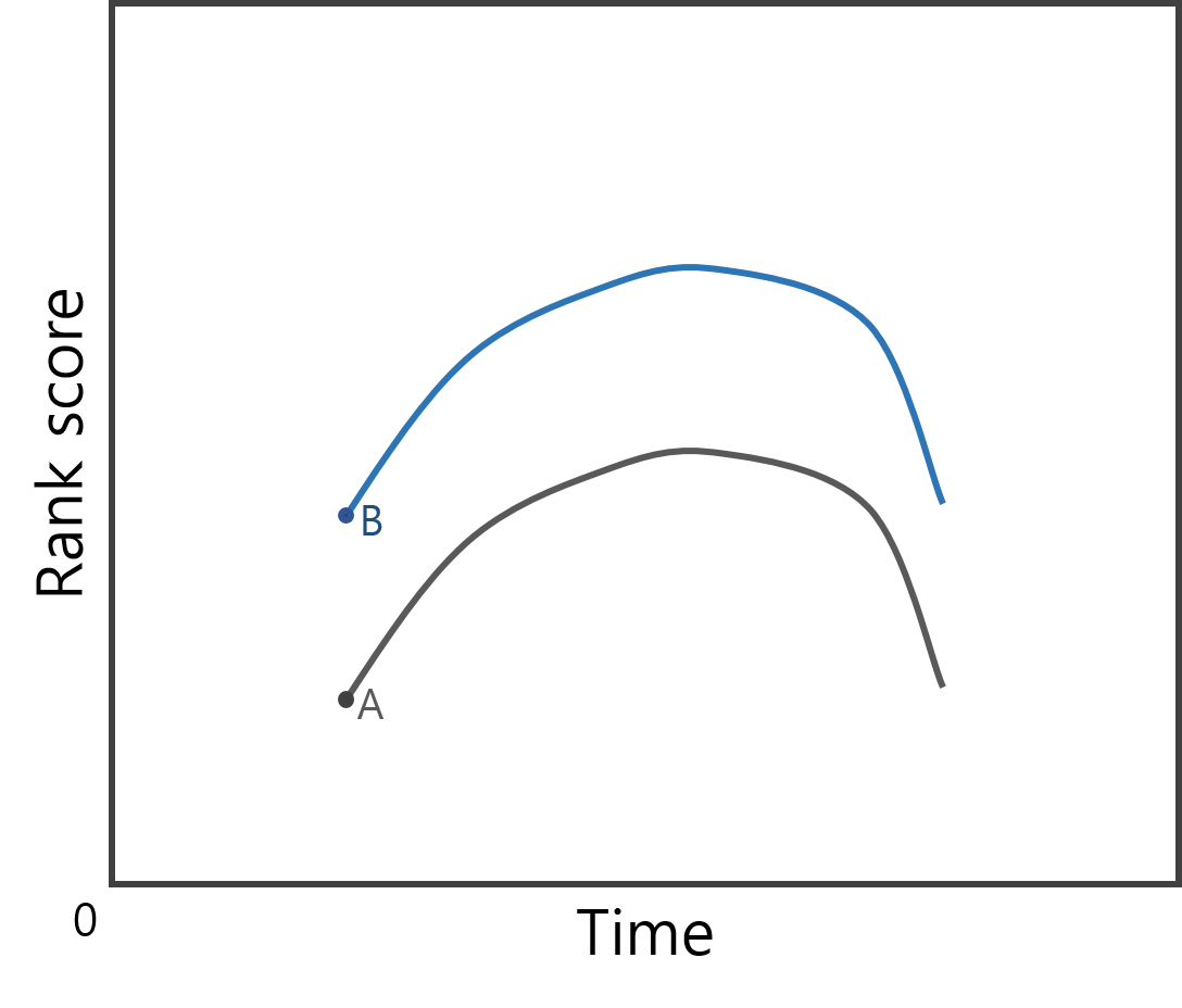
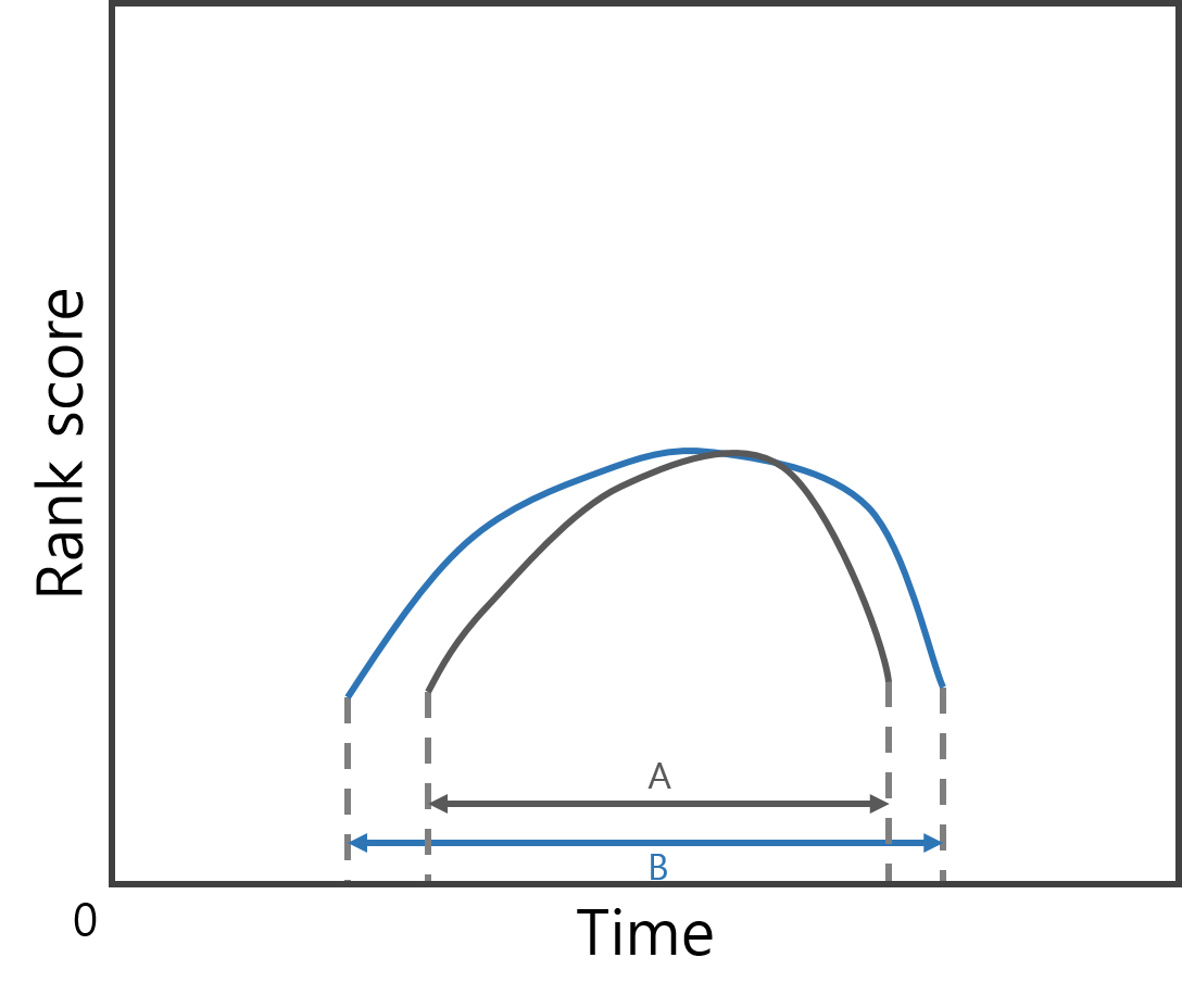
We define eight popularity metrics as follows (see Figure 1):
-
Debut
This is defined as the rank score of a song when the song appears first in a chart. It indicates the initial popularity of the song. In Figure 1a, song B has a larger value of Debut than song A.
-
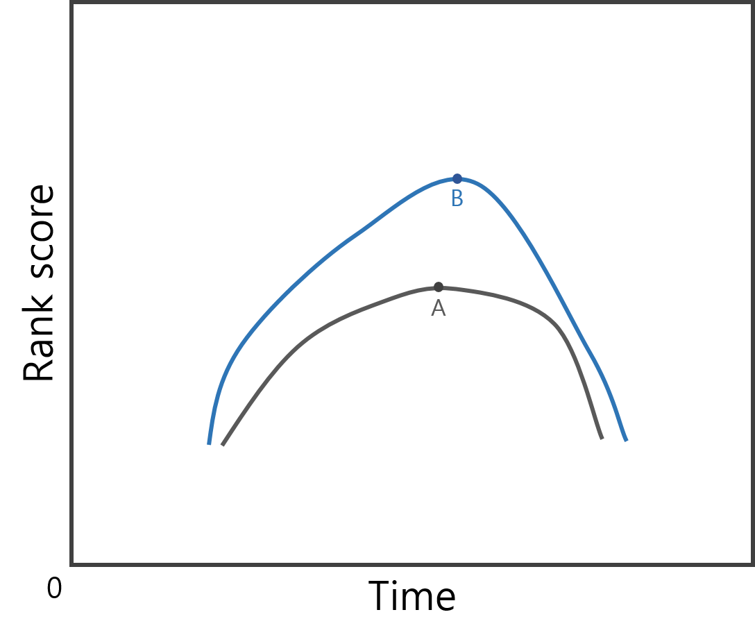
Max
This is defined as the maximum rank score of a song during the whole period, measuring the maximum popularity of the song. The maximum rank score of song B is higher than that of song A in Figure 1b and thus song B has a larger value of Max than song A.
-
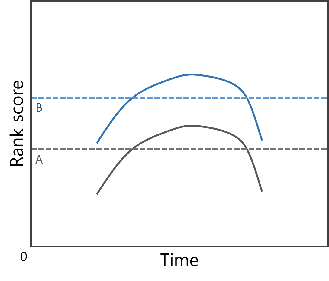
Mean
This is defined as the average rank score of a song over the whole period during which the song appears in a chart. In Figure 1c, song B has a larger value of Mean than song A (marked with dotted lines).
-
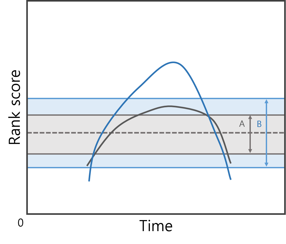
Std
This is the standard deviation of the rank scores of a song over the whole period during which the song appears in a chart. It describes how much the popularity of a song has changed over time. In Figure 1d, the rank score of song B has changed more, so its value of Std is larger than that of song A.
-
Length
This is defined as the time period (e.g., the number of weeks) during which a song appears on a chart. It measures how long a song has been popular, and thus can identify steadily popular songs. In Figure 1e, song B has a larger value of Length than song A.
-
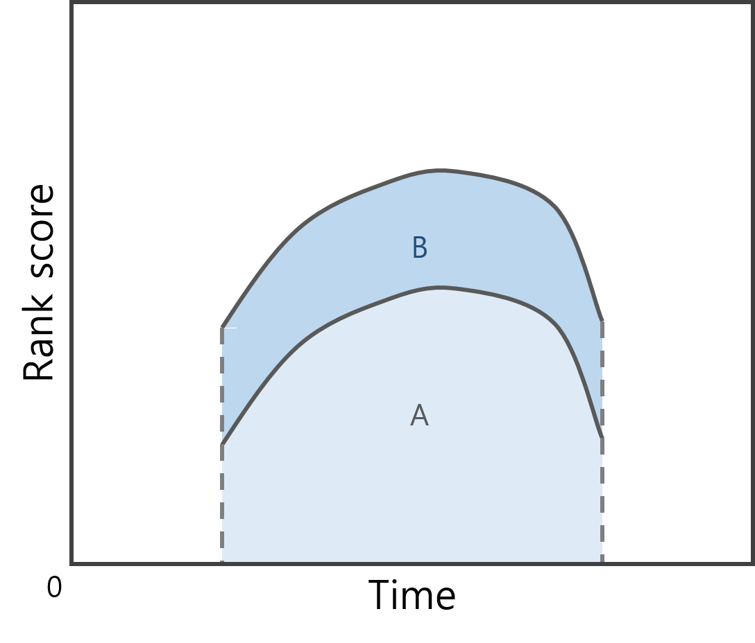
Sum
This is defined as the sum of the rank scores over time. Although this is similar to Length, Length measures only the time period, whereas, Sum considers the rank score during which a song stays in a chart. Thus, it basically describes the overall popularity of a song when the whole time period is considered. In Figure 1f, song B always has higher scores, so the value of Sum of song B is larger than that of song A. Note that Sum is different from Mean because the period during which a song appears in a chart is different for different songs.
-
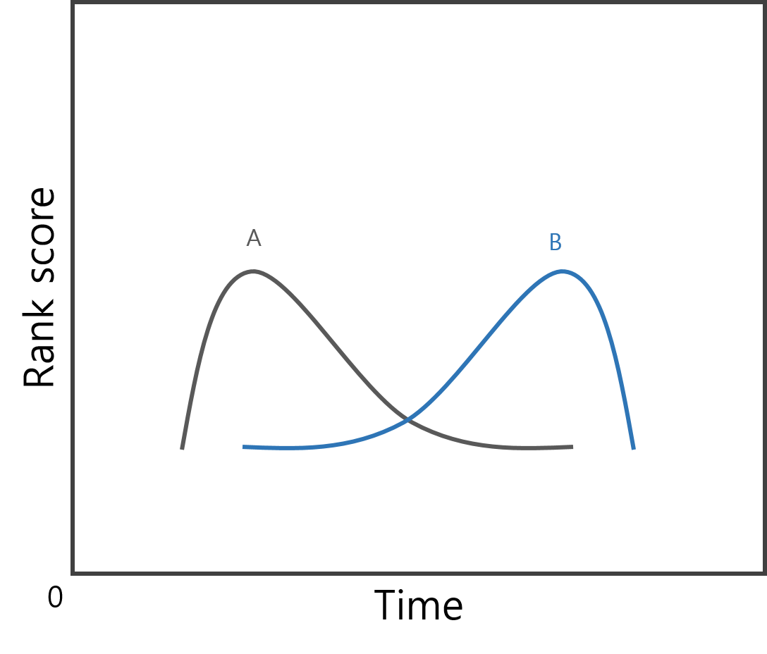
Skewness
This is the skewness (i.e., the third moment) of the rank scores of a song. This partially describes the dynamic patterns that a song gains and loses popularity. A positive value of Skewness (song A in Figure 1g) means that the song has become popular fast, reached its highest popularity, and become unpopular slowly; a negative value of Skewness (song B in Figure 1g) indicates that the song has become popular slowly, then lost its popularity fast.
-
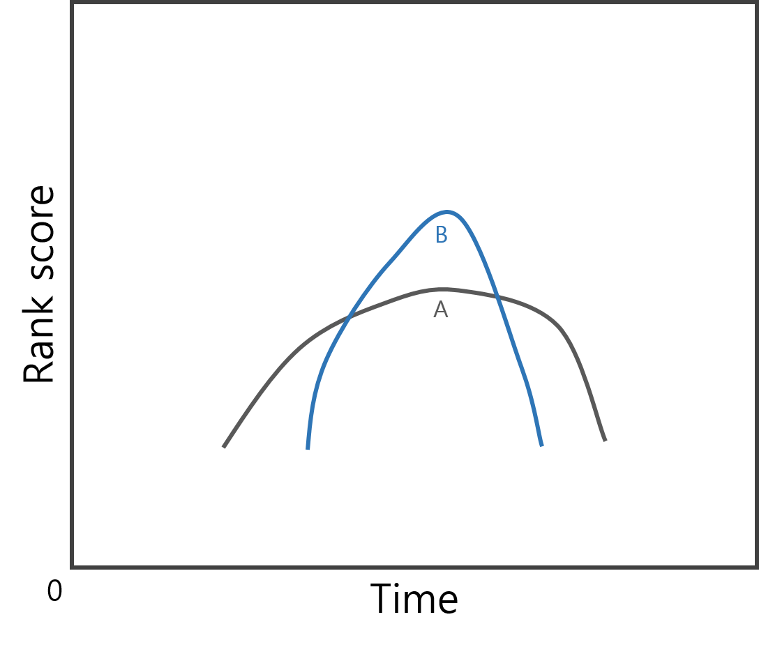
Kurtosis
Together with Skewness, the kurtosis of a song describes the patterns of growing and declining popularity. The faster the popularity growth of a song is, the larger the value of Kurtosis is. The rank score curve for song B in Figure 1h is sharper than that of song A, so Kurtosis of song B is larger.
III Analysis of popularity metrics
III-A Data
The Billboard magazine distributes weekly lists of popular songs, called the Billboard charts, since 1940. The Billboard Hot 100 chart111http://www.billboard.com/charts/hot-100 is the most representative among the charts, which provides 100 most popular songs (regardless of their genres) every week. The ranking in this chart is based on radio airplay, sales data, and streaming activity data from Nielsen Music222http://www.nielsen.com/us/en/solutions/measurement/music-sales-measurement.html.
We use the chart data between 1970 and 2014, comprising 209,000 chart ranks for 2,090 weeks in total. There are 18,604 distinct songs in these data. We exclude the songs that appeared only one or two weeks because some popularity metrics cannot be obtained reliably for them. The number of songs remained only one and two weeks are 1,077 and 841, respectively. Finally, we use the chart data of the remaining 16,686 songs.
III-B Distribution analysis
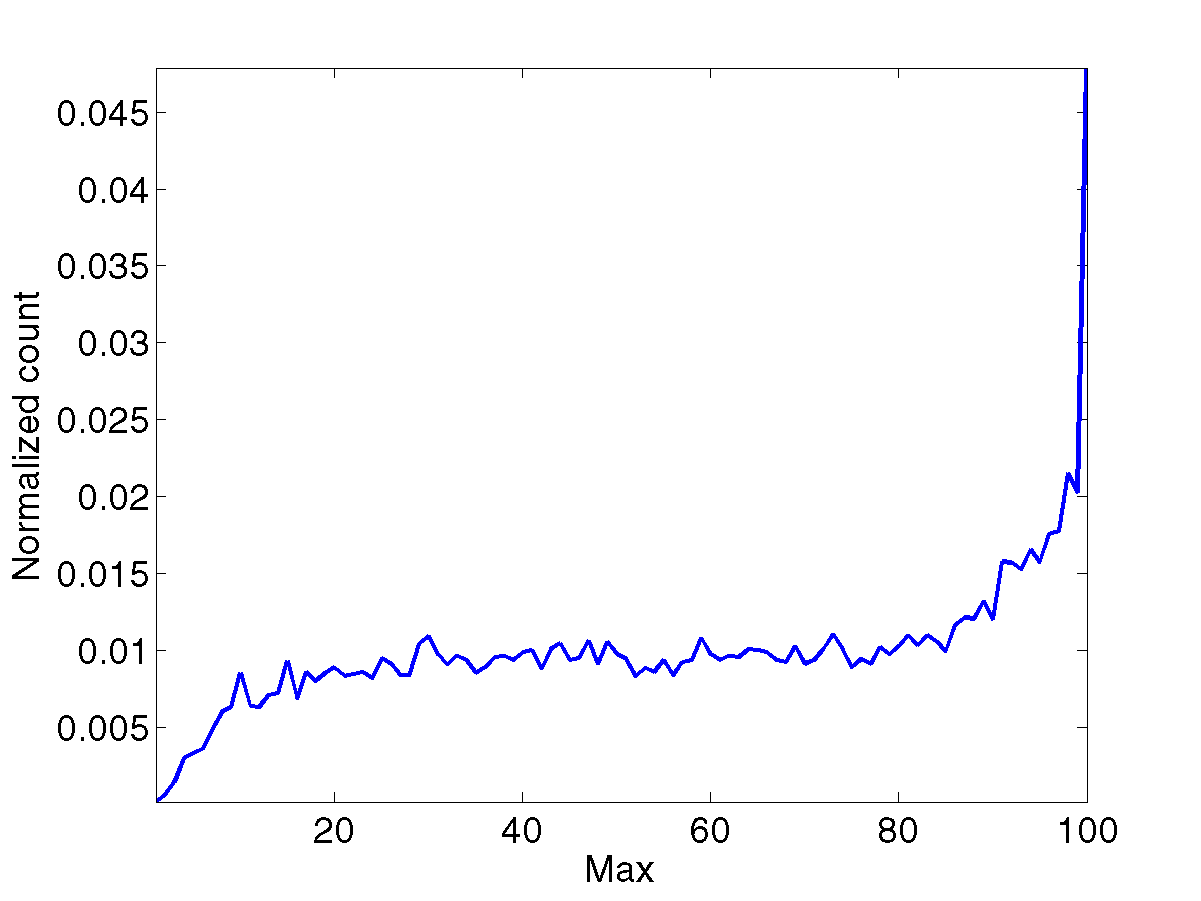
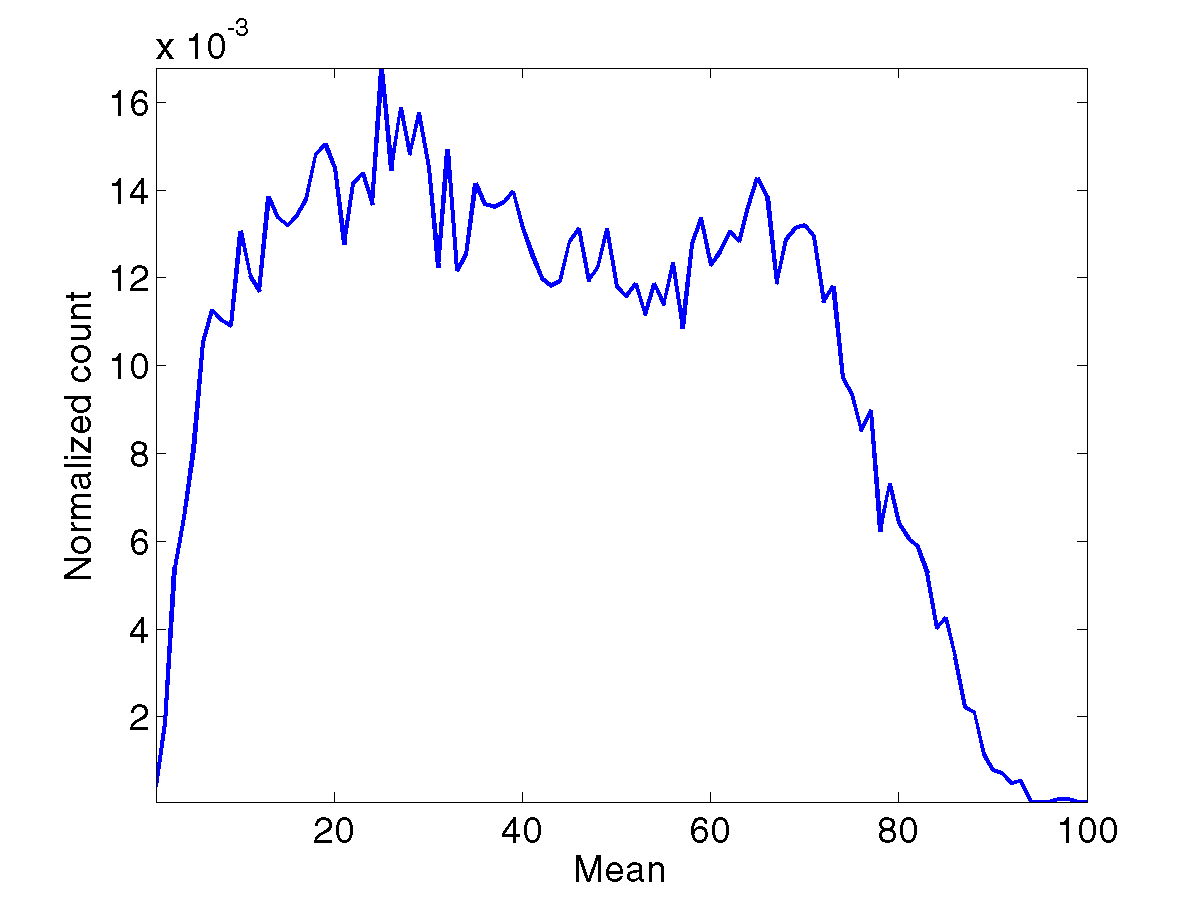
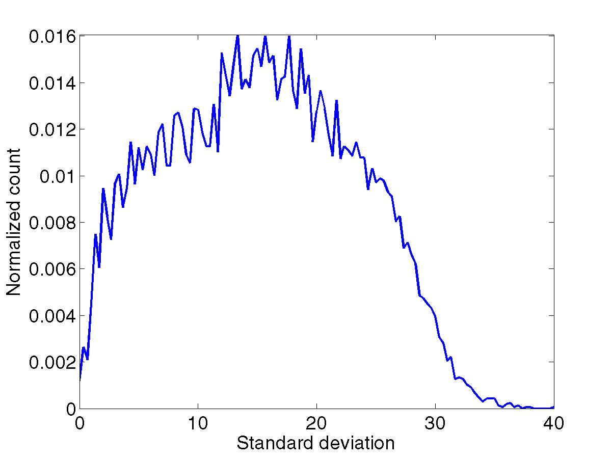
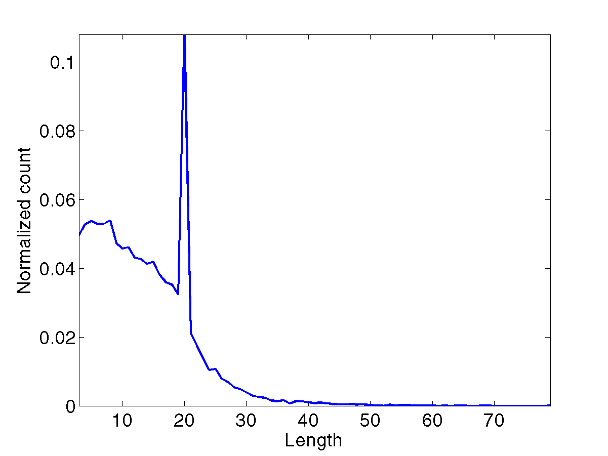
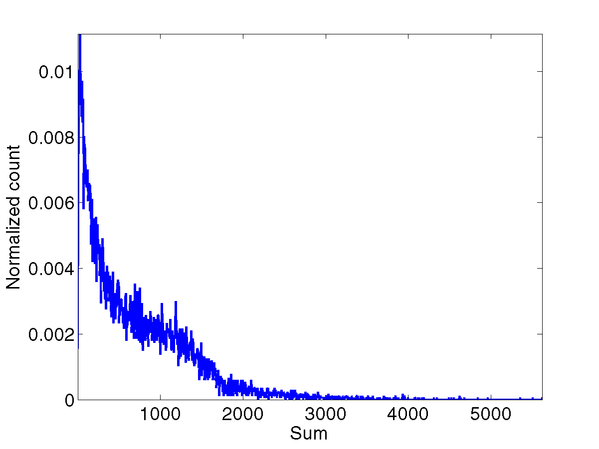
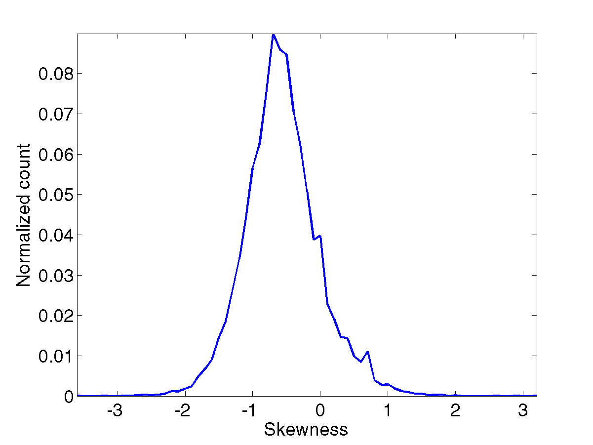
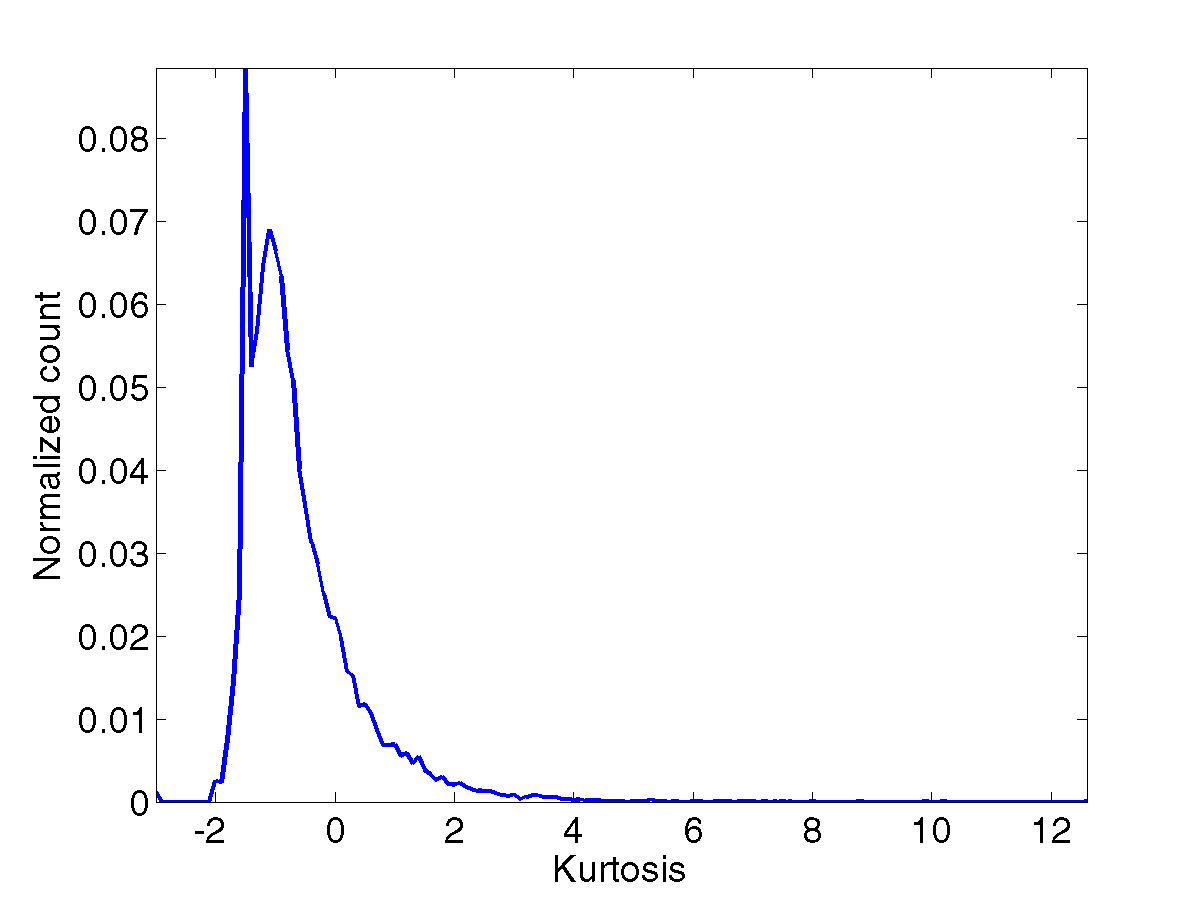
Figure 2 shows the histograms of the eight popularity metrics for the whole chart data set.
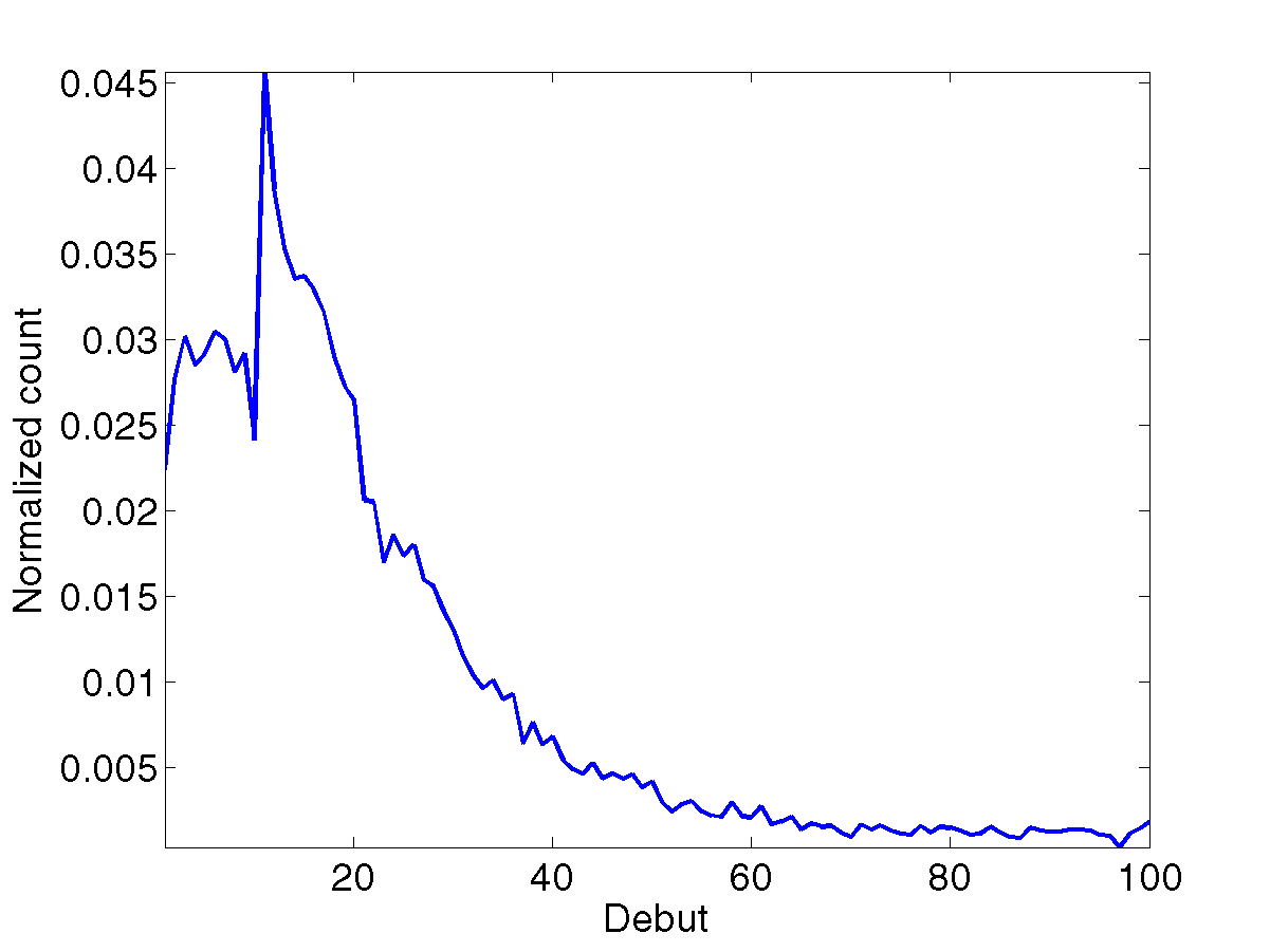
The histogram of Debut in Figure 2a shows that most of the songs were ranked low when they appeared in the chart for the first time. The mean and median values of Debut are 21.8 and 16, respectively. A peak at a rank score of 11 (i.e., 90th in the chart) is also observed in the histogram. Only a small number of songs were ranked high at the beginning; 8.1% of the songs received Debut scores larger than 50 (i.e., ranks higher than 51). There also exist songs debuted as their highest ranking (less than 0.2%).
However, in Figure 2b, the histogram of Max is concentrated in the region with high values; a peak at 100 (i.e., the top rank in the chart) is observed, showing that more than 4.5% of songs reached the top rank. Then, the histogram is almost flat over a wide range between about 20 and 80.
The histogram of Mean is roughly flat in the mid-range (Figure 2c). The mean and median values are 42.1 and 41, respectively, meaning that the average ranks of the songs are slightly lower than the middle in the chart. In Figure 2d, Std is distributed over a large range, with a mean of 15.3. Its maximum value is 39.9, which is relatively large.
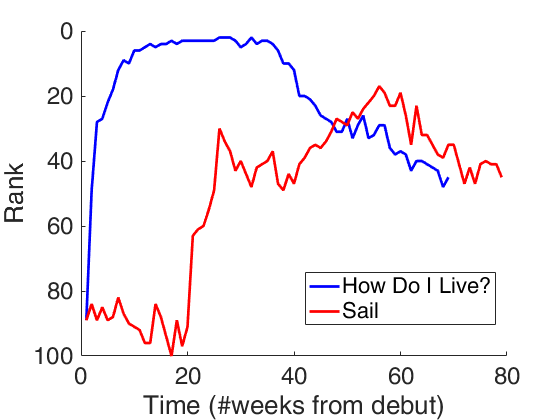
Figure 2e shows that the histogram of Length is concentrated on small values. On average, the songs remained in the chart for 13.4 weeks. A sharp peak at 20 weeks is observed. This is due to the recurrent rule333http://www.billboard.com/biz/billboard-charts-legend, which removes songs ranked below a half (50 in our case) for more than 20 weeks from the chart. The maximum value is 79 weeks, which corresponds to “Sail” by AWOLNATION, 2011.
The histogram in Figure 2f shows that many songs have small values of Sum, and a few songs have extremely large values. As a result, the median and average values differ largely: 506 and 682.2, respectively. The maximum Sum value is 5,615 (“How Do I Live?” by LeAnn Rimes, 1997). Thus, the song with the maximum value of Sum and that with the maximum value of Length are different. The ranks of these two songs over time are shown in Figure 3. The song “Sail” stayed longer in the chart but was ranked lower than the song “How do I live?” overall, which resulted in a lower value of Sum of the former than the latter. This justifies the necessity of observing both Sum and Length as popularity metrics.
The histogram of Skewness in Figure 2g is similar to the probability density function of a Laplace distribution, with a peak at -0.7. This shows that on average, the popularity of a song typically grows slowly and falls fast.
The histogram of Kurtosis is also peaked at a negative value, as shown in Figure 2h. The mean value of Kurtosis is -0.62, and most of the songs have negative Kurtosis values, indicating that the degree of peakedness of the growth and decline of the popularity is flatter than that of the normal distribution. Nevertheless, there also exist songs that have extremely large positive values of Kurtosis, which gained and lost their popularity very quickly.
III-C Effects of debut performance
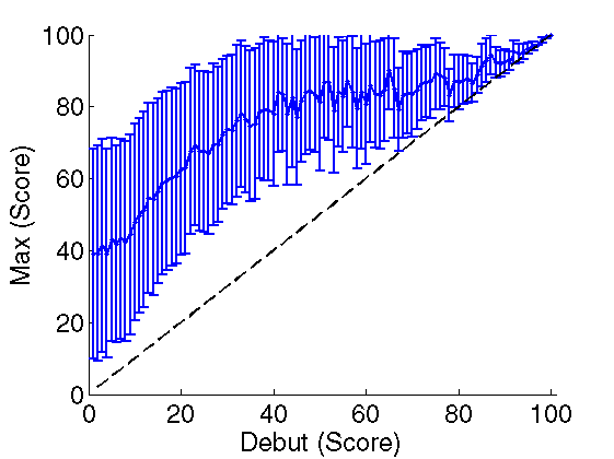
We now focus on the effects of the initial chart performance of a song, i.e., Debut. First, we examine the relationship between Debut and Max in Figure 4. It is observed that the Debut performance of a song significantly influences its best chart performance. It is usually hard to reach high ranks for a song with a low initial rank, but once the initial rank is higher than about 50, then the best performance does not vary much.
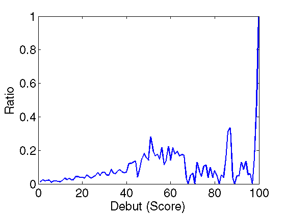
Next, we examine the proportion of the number of songs reaching the highest rank (i.e., #1) in the chart with respect to Debut. The result is shown in Figure 5. For the songs whose debut ranks are below a half (i.e., 50), the probability of reaching the top in the chart gradually increases with respect to the debut rank. However, once the debut rank is above a half, no significant correlation is observed between the debut rank and the probability of reaching the top. Surprisingly, only a half of the songs that debuted in second place in the chart succeeded in reaching the top.
III-D Temporal analysis
We examine how the popularity metrics changed over time. For this, we set four decadal periods, i.e., 1970s, 1980s, 1990s, and 2000s, and obtain the popularity metrics separately for each period. Only the songs that appeared and disappeared in the chart within the same period were considered. As a result, 5,074, 4,192, 3,570, and 4,375 songs were included in the four periods, respectively.
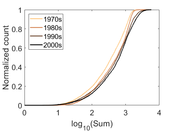
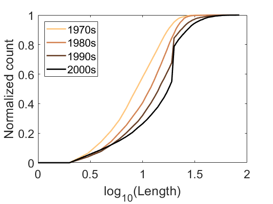
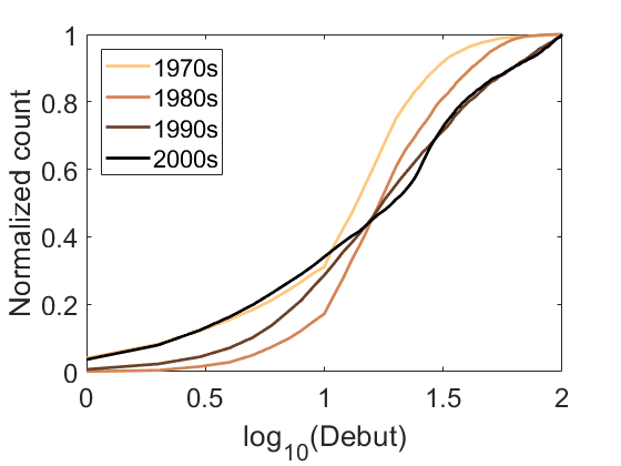
Figure 6 shows the cumulative distributions of Sum, Length, and Debut. Those for the other popularity metrics are omitted because they do not show any noticeable difference among different periods. It is observed that a larger portion of songs have larger Sum and Length values as time goes. Larger values of Length for more recent decades would be partially responsible for the increase of the proportion of large values of Sum. In Figure 6b, abrupt increases at week 20 are observed only for 1990s and 2000s, because the recurrent rule has applied only after 1991. In Figure 6c, the distribution of Debut becomes more gradual as time goes. To sum up, songs in more recent years tend to have appeared in the chart at more various initial ranks and stayed longer in the chart.
IV Prediction of Popularity Metrics
We build models that predict the popularity metrics using musical features. The complexity features, and two other types of acoustic features used in previous studies are explained. Then, the experimental setup and results are presented.
IV-A Comlexity features
As described in [19, 20], music complexity is highly involved in determining preference and popularity of a song. Therefore, we measure complexity of songs and use them to build learning models. In particular, we adopt the method presented in [29], which measures structural changes of three musical components, namely, harmonic, rhythmic, and timbral components of a song. The method extracts these components from a song, and then calculates complexity features by measuring temporal changes of the components. In addition, we consider loudness as another dimension reflecting music complexity, because loudness of a song and its temporal change are related to emotional arousal of listeners.
IV-A1 Structural change
The structural change (SC) [29] basically measures how fast the time sequence of a component changes over time. Three components are considered as follows.
- Chroma
-
Chroma describes the instantaneous harmony at a particular moment, which is one of the 12 chords (C, C#, D, …, B). For each signal segment having a length of 0.25 sec, we use the chord estimation algorithm presented in [30] to obtain the probability distribution over the 12 chords.
- Rhythm
-
We employ the fluctuation pattern (FP) [31] to quantify the rhythmic signature at a certain moment in a song. A 2.97 second-long Hamming window moving one second at a time is applied to the audio signal. The windowed audio segment is further divided into 256 frames (containing 512 samples for 44.1 kHz sampling). For each frame, the fast Fourier transform (FFT) is applied and the periodicity histogram [31] of each frequency band is measured to obtain FPs of the frames. The mean of the 256 FPs is defined as the rhythm component of the segment.
- Timbre
-
The timbral components of a song are mostly determined by its frequency components. Thus, we employ the Mel-frequency cepstral coefficients (MFCCs) [32] that are popular for perceptual representation of spectral aspects of audio signals. As in the case of rhythm, we apply a 2.97 second-long Hamming window to the given audio signal and then divide the windowed segment into 256 frames. We use 36 Mel-frequency spaced bins for each frame. Finally, the MFCCs from the 256 frames are averaged.
We compute SC on each component to obtain complexity features over time. The SC for the th segment with an observation window having a length of is given by
| (2) |
where is the Jenson-Shannon divergence between and and is the sum of the values of for the th to th segments. The observation window determines the temporal scope measuring complexity. We set for chroma and for rhythm and timbre, which correspond to window lengths of 1 to 32 sec. Finally, we take the mean value of SC over time to obtain a single value for each feature and each window size. As a result, six complexity features for the six observation window lengths are obtained for each of the Chroma, Rhythm, and Timbre components: Chroma1 to Chroma6, Rhythm1 to Rhythm6, and Timbre1 to Timbre6.
IV-A2 Arousal
We use another kind of complexity feature based on the psychoacoustic theory, named Arousal. It has been known that the loudness of music is correlated to the arousal dimension of emotion [33]. And, emotion is an important factor determining music preference [34]. Therefore, we can assume that the musical preference (and consequently music popularity) is influenced by arousal.
We calculate the short-time magnitude (i.e., sum of the absolute signal values) for a segment obtained using a 2.97-second long Hamming window moving one second at a time. We then calculate the mean (ArousalMean) and standard deviation (ArousalStd) of the short-time magnitudes over time to measure the average and variation of loudness, respectively.
IV-B MPEG features
The MPEG-7 Audio standard444http://mpeg.chiariglione.org/standards/mpeg-7/audio provides tools to measure various spectral and temporal characteristics of audio signals. MPEG-7 Audio features are extracted by using the bag-of-frame (BOF) approach, which divides the audio signal into segments, extracts audio features, and summarizes all segments using statistical measures such as sum and standard deviation. We use the MPEG-7 Reference Software555http://mpeg.chiariglione.org/standards/mpeg-7/reference-software to obtain 82 MPEG-7 Audio features from each song.
IV-C MFCC features
In [21], features based on MFCCs were used to measure the spectral characteristics of songs for hit song prediction. We also employ them by implementing the feature extraction procedure in [21]. Each audio signal is divided into segments having a length of 0.025 sec with an overlap of 0.015 sec between adjacent segments, and 20 MFCCs are extracted for each segment. For the extracted MFCCs of the songs in the training data set, k-means clustering is conducted, from which 32 cluster centroids are obtained, in order to reduce noise and obtain compact features. These centroids represent the most common sound characteristics found in the training data. When a song for test is given, the minimum distance centroids for its MFCC vectors are found and the normalized frequencies of the 32 clusters are obtained as the features of the song.
IV-D Experimental setup
IV-D1 Data
Listeners’ preference to songs tends to change over time (e.g., popular genres in different periods). In addition, as shown in Section III-D, the trends for some popularity metrics have changed. Thus, popularity prediction over a long time period such as several decades would not be of much interest. Considering this, we conduct our experiments with the songs within the recent five years. Specifically, the 1,264 songs appearing in the Billboard Hot 100 chart during 253 weeks between 13 June 2009 and 19 April 2014 are used for our experiments. The first 70% of the period, until 11 November 2012 (including 864 songs), is considered for training classifiers, the first half of the rest (200 songs) for validation, and the last half (200 songs) for testing. In other words, we examine whether the prediction of “future popularity” is feasible.
IV-D2 Setup
We use support vector machines (SVMs) as classifiers666We present only the results of the most effective classifier in this section, but complete results using other classifiers are shown in Appendix.. We train SVMs with the extracted features to perform binary classification of each popularity metric. The boundary of the two classes is set to the median value of each popularity metric in the training data set. The radial basis function (RBF) is used as the kernel function of the SVMs. The values of the penalty factor and the width of the RBF function determined empirically for the validation dataset. We use the libsvm package777https://www.csie.ntu.edu.tw/~cjlin/libsvm/ [35].
We design three different experiments to investigate popularity prediction performance of the features:
-
1.
Prediction using each single complexity feature
-
2.
Prediction using each feature group
-
3.
Prediction using combined features.
In the first experiment, the classifier is trained with a single feature to examine whether each complexity feature can predict popularity metrics and which feature is effective for prediction. The second experiment compares the prediction performance of each feature group, i.e., Complexity, MPEG, and MFCC. Finally, the third experiment examines performance improvement by additional use of MFCC and/or MPEG together with Complexity.
In order to compensate for different numbers of data in the two classes, the classification performance is measured in terms of the balanced accuracy, which is defined as
| (3) |
where , , , and are the numbers of true positives (hit), true negatives (correct rejection), false positives (false alarm), and false negatives (miss), respectively.
IV-E Results
IV-E1 Single feature-based prediction
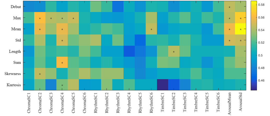
Figure 7 summarizes the prediction results using single Complexity features. One-sided t-tests are conducted to examine if the balanced accuracies are significantly different from the random chance (i.e., 0.5). The cases showing statistical significance are marked with ‘*’ in the figure. In total, 11.9% of all cases are shown to be statistically significant, which indicates that some complexity features are effective for predicting popularity metrics even when used singly.
Among the four components of complexity, features from Chroma (ChromaSC1 to ChromaSC6) are the most effective; 20.8% of the cases using the chroma-based features show statistically significant performance. The Rhythm and Timbre features are not as effective as the Chroma features. Interestingly, the Arousal features, which are based on simple loudness measurement, perform well, showing significant performance for Debut, Max, Mean, and Std.
Chroma is related to the flow of a song such as melody, mood, and chord, and listeners prefer appropriate change of such flow. Although Rhythm and Timbre features are less effective, they are complementary with each other; the features from Timbre are effective for predicting Length, while those from Rhythm are effective for Mean.
In the viewpoint of popularity metrics, Debut and Kurtosis are difficult to predict with single Complexity features. Only Arousal features are effective for Debut.
When the performance with respect to the window size is examined, there exists a slight tendency that smaller windows are more effective for Rhythm and Timbre than larger ones, whereas the window size does not affect the performance of Chroma much as long as it is not the smallest or largest. It is thought that rapid changes of rhythm or timbre are easily captured by listeners, thus have impact on the listeners’ preference. However, chromatic changes due to chord alteration over both small and large time scales are expected in most songs, thus a wide range of window sizes appear effective.
IV-E2 Feature group-based prediction
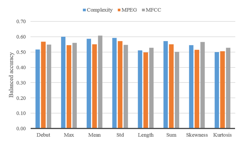
The prediction results of each feature group are shown in Figure 8. For Debut, Length, and Kurtosis, the prediction performance of each feature group is overall inferior to that for the other popularity metrics. In fact, the debut ranking of a song may be more influenced by awareness and popularity of the artist, promotion, or social trend, as in other cultural products [25, 36, 37].
The group of Complexity is the most effective among the three groups in predicting Max, Std, and Sum, for which relatively good performance was observed in Figure 7. MFCC shows the best prediction performance for Length, Mean, Skewness, and Kurtosis, although the accuracies are not high for Length and Kurtosis. MPEG ranks first only for Debut.
These results demonstrate that the Complexity features capture popularity-related characteristics of songs more effectively than the MFCC and MPEG features that are designed to extract rather general acoustic characteristics. Complexity and MFCC showing better performance than MPEG, perceptual features are more suitable for popularity prediction.
IV-E3 Prediction using combined features
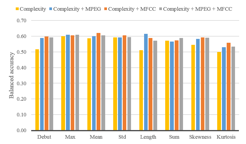
| Complexity | |||
|---|---|---|---|
| hit | miss | ||
| MFCC | hit | 0.391 | 0.176 |
| miss | 0.176 | 0.258 | |
Table I shows the confusion matrix examining how Complexity and MFCC behave in feature group-based prediction. The cases where one group produces correct classification results but the other does not take about 35% (the off-diagonal elements in the matrix), for which we can expect complementarity when they are combined.
Figure 9 summarizes the balanced accuracies of prediction when the MPEG and MFCC features are combined with the Complexity features. In most cases, additional use of MPEG and/or MFCC improves the performance. In particular, the improvement is prominent for Debut, Length, and Kurtosis. Overall, the combination of Complexity and MFCC appears the best, recording an average accuracy of 59.2%. Further combination of MPEG deteriorates the performance in most cases, which seems to be due to the excessively increased feature dimensionality.
The accuracies in Figure 9 may look quite low. But it is thought that the problem of popularity prediction is very challenging, as also shown in previous studies. For instance, in [21], a problem of classifying whether a song will rank first was considered, for which relatively low performance was reported (0.66 in terms of area under curve (ROC)). In [22], no statistically significant performance in comparison to random chance was obtained for a three-class popularity classification problem. In our case, on the other hand, one-sided t-tests reveal that the accuracies for Complexity+MFCC are statistically significant except for Kurtosis.
IV-E4 Incorporating Debut as a feature
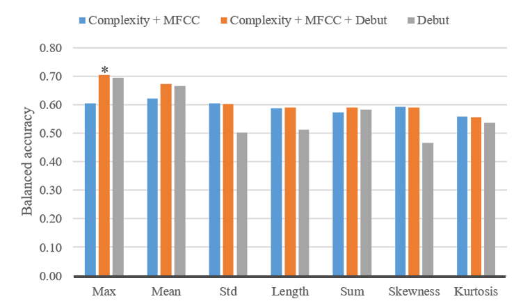
Finally, we examine a different scenario, where popularity metrics of a song are predicted after it has debuted in the chart. While the acoustic features-based popularity prediction shown above are useful even before a song is released to the public, it is also interesting how the popularity of a song will evolve once we know its debut performance in the chart.
For this, the debut score of a song is used as a feature in addition to the acoustic features for prediction. Since the combination of Complexity and MFCC showed the best performance in Figure 9, we evaluate the performance of the combination of Complexity, MFCC, and Debut, which is shown in Figure 10. A significant increase of the accuracy is observed for Max (absolute improvement by 9.9%) due to the additional use of the debut score. The strong correlation between Debut and Max, which was shown in Figure 4, and thereby a high accuracy using even only Debut for Max, seems to contribute to the performance improvement. We also observe slight performance improvement for Mean. For the rest, there is almost no performance difference.
V Conclusions
In this paper, we have defined popularity metrics, analyzed their properties from real chart data, and automatically predicted them using acoustic features. To consider various aspects of popularity, we defined eight popularity metrics: Debut, Max, Mean, Std, Length, Sum, Skewness, and Kurtosis from rankings of a song in the chart, which are complementary with each other.
We examined the characteristics of the popularity metrics with the real chart data for 16,686 songs ranked in the Billboard Hot 100 chart between 1970 and 2014. Each popularity metric showed a distinct distribution, from which noteworthy observations were made. Most songs scored low ranks at the beginning in the chart. Although many songs reached the highest rank at least once, their average scores were distributed in the middle range of the chart. The growth pattern of popularity was usually gradual, rising slowly and falling quickly. The maximum rank of a song was highly related to its debut performance. We also investigated the popularity metrics in different decades. It was observed that in more recent years, more songs debuted in the chart and stayed longer.
Prediction of the popularity metrics was conducted using acoustic features. We proposed to use Complexity features including musical and arousal components for popularity prediction based on the theory describing close relationship between complexity and preference. We performed binary classification using SVMs with 1,264 songs in the Billboard Hot 100 chart for 253 weeks. Single features from Chroma and Arousal performed well, which indicates that these components are related to preference of listeners. Overall, Complexity was superior to MFCC and MPEG. Combining Complexity and MFCC improved prediction performance for most popularity metrics. It was also shown that the information of the debut score is effective to increase further the accuracy for Max.
To sum up, we have investigated what popularity of a song is, how the popularity metrics look in the real world, and whether they are predictable using acoustic features. In the future, it would be necessary to attempt to improve the prediction performance, e.g., using deep neural networks.
| Classifier | Feature | Debut | Max | Mean | Std | Length | Sum | Skewness | Kurtosis |
|---|---|---|---|---|---|---|---|---|---|
| SVM | Complexity | 0.52 | 0.60 | 0.59 | 0.59 | 0.51 | 0.57 | 0.54 | 0.50 |
| MPEG | 0.57 | 0.54 | 0.55 | 0.57 | 0.50 | 0.55 | 0.51 | 0.51 | |
| MFCC | 0.55 | 0.56 | 0.61 | 0.55 | 0.53 | 0.50 | 0.57 | 0.53 | |
| LR | Complexity | 0.51 | 0.59 | 0.60 | 0.57 | 0.57 | 0.56 | 0.52 | 0.50 |
| MPEG | 0.47 | 0.49 | 0.50 | 0.48 | 0.55 | 0.54 | 0.47 | 0.47 | |
| MFCC | 0.53 | 0.56 | 0.59 | 0.53 | 0.54 | 0.56 | 0.61 | 0.48 | |
| DT | Complexity | 0.52 | 0.51 | 0.60 | 0.48 | 0.47 | 0.47 | 0.47 | 0.41 |
| MPEG | 0.53 | 0.56 | 0.55 | 0.49 | 0.48 | 0.55 | 0.46 | 0.56 | |
| MFCC | 0.53 | 0.49 | 0.54 | 0.51 | 0.50 | 0.53 | 0.49 | 0.50 | |
| NN | Complexity | 0.45 | 0.51 | 0.56 | 0.50 | 0.55 | 0.52 | 0.57 | 0.49 |
| MPEG | 0.49 | 0.53 | 0.54 | 0.57 | 0.53 | 0.50 | 0.48 | 0.52 | |
| MFCC | 0.56 | 0.59 | 0.55 | 0.53 | 0.47 | 0.50 | 0.54 | 0.53 | |
| CNN | 0.52 | 0.52 | 0.53 | 0.48 | 0.49 | 0.55 | 0.48 | 0.53 |
We present the complete results of feature group-based popularity metric prediction using various classifiers. The employed classifiers are decision tree (DT), logistic regression (LR), neural network with a single hidden layer having sigmoidal neurons (NN), and CNN. The number of hidden neurons in NN is determined empirically for the validation dataset. NN is trained with the Levenberg-Marquardt algorithm that is one of the fastest learning algorithms. For the CNN, the model presented in [23] was adopted, where a fully connected layer is used for the final layer. The input of the CNN is the 128-band Mel-spectrogram of the 120-second-long middle part of each audio signal.
The performance in terms of balanced accuracy of each classifier is shown in Table II. On average, SVM shows the best performance among the classifiers with consistently good accuracies for the three types of features when all the popularity metrics are considered, although some classifiers show better performance for some cases (e.g., LR using MFCC for Skewness). The deep learning approach performs poor, probably due to the insufficient amount of data for training.
References
- [1] J. Lee and J.-S. Lee, “Predicting music popularity patterns based on musical complexity and early stage popularity,” in Proc. Third Workshop on Speech, Language & Audio in Multimedia, 2015, pp. 3–6.
- [2] S. D. Roy, T. Mei, W. Zeng, and S. Li, “Towards cross-domain learning for social video popularity prediction,” IEEE Trans. Multimedia, vol. 15, no. 6, pp. 1255–1267, Oct. 2013.
- [3] T. Trzciński and P. Rokita, “Predicting popularity of online videos using support vector regression,” IEEE Trans. Multimedia, vol. 19, no. 11, pp. 2561–2570, Nov. 2017.
- [4] Y. Zhou, L. Chen, C. Yang, and D. M. Chiu, “Video popularity dynamics and its implication for replication,” IEEE Trans. Multimedia, vol. 17, no. 8, pp. 1273–1285, Aug. 2015.
- [5] J. Wu, Y. Zhou, D. M. Chiu, and Z. Zhu, “Modeling dynamics of online video popularity,” IEEE Trans. Multimedia, vol. 18, no. 9, pp. 1882–1895, Sept. 2016.
- [6] S. Rudinac, M. Larson, and A. Hanjalic, “Learning crowdsourced user preferences for visual summarization of image collections,” IEEE Trans. Multimedia, vol. 15, no. 6, pp. 1231–1243, Oct. 2013.
- [7] S. Huang, J. Zhang, L. Wang, and X. S. Hua, “Social friend recommendation based on multiple network correlation,” IEEE Trans. Multimedia, vol. 18, no. 2, pp. 287–299, Feb. 2016.
- [8] S. Traverso, M. Ahmed, M. Garetto, P. Giaccone, E. Leonardi, and S. Niccolini, “Unravelling the impact of temporal and geographical locality in content caching systems,” IEEE Trans. Multimedia, vol. 17, no. 10, pp. 1839–1854, Oct. 2015.
- [9] J. P. Friedlander, “News and notes on 2013 RIAA music industry shipment and revenue statistics,” Recording Industry Association of America, Tech. Rep., 2014.
- [10] H.-C. Chen and A. L. Chen, “A music recommendation system based on music data grouping and user interests,” in Proc. Tenth Int. Conf. Inf. Knowledge Manag., 2001, pp. 231–238.
- [11] J.-J. Aucouturier and F. Pachet, “Scaling up music playlist generation,” in Proc. IEEE Int. Conf. Multimedia Expo, vol. 1, 2002, pp. 105–108.
- [12] B. Logan, “Music recommendation from song sets.” in Proc. Int. Soc. Music Inf. Retrieval Conf., 2004, pp. 425–428.
- [13] F.-F. Kuo, M.-F. Chiang, M.-K. Shan, and S.-Y. Lee, “Emotion-based music recommendation by association discovery from film music,” in Proc. 13th ACM Int. Conf. Multimedia, 2005, pp. 507–510.
- [14] D. Eck, P. Lamere, T. Bertin-Mahieux, and S. Green, “Automatic generation of social tags for music recommendation,” in Advances in Neural Information Processing Systems, 2008, pp. 385–392.
- [15] K. Lee and K. Lee, “Using dynamically promoted experts for music recommendation,” IEEE Trans. Multimedia, vol. 16, no. 5, pp. 1201–1210, Aug. 2014.
- [16] R. M. MacCallum, M. Mauch, A. Burt, and A. M. Leroi, “Evolution of music by public choice,” Proc. Natl. Acad. Sci. U.S.A, vol. 109, no. 30, pp. 12 081–12 086, 2012.
- [17] J. Serrà, Á. Corral, M. Boguñá, M. Haro, and J. L. Arcos, “Measuring the evolution of contemporary western popular music,” Scientific Reports, vol. 2, pp. 521:1–6, 2012.
- [18] M. Mauch, R. M. MacCallum, M. Levy, and A. M. Leroi, “The evolution of popular music: USA 1960–2010,” Royal Society Open Science, vol. 2, no. 5, pp. 150 081:1–10, 2015.
- [19] L. Steck and P. Machotka, “Preference for musical complexity: Effects of context,” Journal of Experimental Psychology: Human Perception and Performance, vol. 1, no. 2, pp. 170–174, 1975.
- [20] R. M. Parry, “Musical complexity and top 40 chart performance,” Tech. Rep., 2004.
- [21] R. Dhanaraj and B. Logan, “Automatic prediction of hit songs.” in Proc. Int. Soc. Music Inf. Retrieval Conf., 2005, pp. 488–491.
- [22] F. Pachet, “Hit song science,” in Music Data Mining. Chapman & Hall/CRC Press Boca Raton, FL, 2012, ch. 10, pp. 305–326.
- [23] L.-C. Yang, S.-Y. Chou, J.-Y. Liu, Y.-H. Yang, and Y.-A. Chen, “Revisiting the problem of audio-based hit song prediction using convolutional neural networks,” in Proc. IEEE Int. Conf. Acoust. Speech Signal Process., Mar. 2017, pp. 621–625.
- [24] L.-C. Yu, Y.-H. Yang, Y.-N. Hung, and Y.-A. Chen, “Hit song prediction for pop music by siamese CNN with ranking loss,” arXiv preprint arXiv:1710.10814, 2017.
- [25] M. J. Salganik, P. S. Dodds, and D. J. Watts, “Experimental study of inequality and unpredictability in an artificial cultural market,” Science, vol. 311, no. 5762, pp. 854–856, 2006.
- [26] T. F. Pettijohn II, G. M. Williams, and T. C. Carter, “Music for the seasons: seasonal music preferences in college students,” Current Psychology, vol. 29, no. 4, pp. 328–345, 2010.
- [27] Z. Ma, A. Sun, and G. Cong, “On predicting the popularity of newly emerging hashtags in Twitter,” J. Am. Soc. for Information Science and Technology, vol. 64, no. 7, pp. 1399–1410, 2013.
- [28] X. Cheng, J. Liu, and C. Dale, “Understanding the characteristics of internet short video sharing: A YouTube-based measurement study,” IEEE Trans. Multimedia, vol. 15, no. 5, pp. 1184–1194, Aug. 2013.
- [29] M. Mauch and M. Levy, “Structural change on multiple time scales as a correlate of musical complexity,” in Proc. Int. Soc. Music Inf. Retrieval Conf., 2011, pp. 489–494.
- [30] M. Mauch and S. Dixon, “Approximate note transcription for the improved identification of difficult chords,” in Proc. Int. Soc. Music Inf. Retrieval Conf., 2010, pp. 135–140.
- [31] E. Pampalk, S. Dixon, and G. Widmer, “On the evaluation of perceptual similarity measures for music,” in Proc. Sixth Int. Conf. Digital Audio Effects, 2003, pp. 7–12.
- [32] P. Mermelstein, “Distance measures for speech recognition, psychological and instrumental,” Pattern Recognition and Artificial Intelligence, vol. 116, pp. 374–388, 1976.
- [33] E. Schubert, “Modeling perceived emotion with continuous musical features,” Music Perception, vol. 21, no. 4, pp. 561–585, 2004.
- [34] T. Schäfer and P. Sedlmeier, “What makes us like music? Determinants of music preference.” Psychol. of Aesthe. Creativity Arts, vol. 4, no. 4, pp. 223–234, 2010.
- [35] C.-C. Chang and C.-J. Lin, “LIBSVM: A library for support vector machines,” ACM Trans. Intelligent Systems and Technology, vol. 2, pp. 27:1–27:27, 2011, software available at http://www.csie.ntu.edu.tw/~cjlin/libsvm.
- [36] F. S. Zufryden, “Linking advertising to box office performance of new film releases-a marketing planning model,” Journal of Advertising Research, vol. 36, no. 4, pp. 29–42, 1996.
- [37] P. K. Chintagunta, S. Gopinath, and S. Venkataraman, “The effects of online user reviews on movie box office performance: Accounting for sequential rollout and aggregation across local markets,” Marketing Science, vol. 29, no. 5, pp. 944–957, 2010.
![[Uncaptioned image]](/html/1812.00551/assets/bio_junghyuklee.jpg) |
Junghyuk Lee received his B.S. degree from the School of Integrated Technology at Yonsei Uni- versity, Korea, in 2015, where he is currently working toward the Ph.D. degree. His research interests include multimedia signal processing and wide color gamut imaging. |
![[Uncaptioned image]](/html/1812.00551/assets/bio_jongseoklee.jpg) |
Jong-Seok Lee (M06-SM14) received his Ph.D. degree in electrical engineering and computer science in 2006 from KAIST, Korea. From 2008 to 2011, he worked as a research scientist at Swiss Federal Institute of Technology in Lausanne (EPFL), Switzerland. Currently, he is an associate professor in the School of Integrated Technology at Yonsei University, Korea. His research interests include multimedia signal processing and machine learning. He is an author or co-author of over 100 publications. He serves as an editor for the IEEE Communications Magazine and Signal Processing: Image Communication. |