Towards Theoretical Understanding of Large Batch Training in Stochastic Gradient Descent

Xiaowu Dai  and  Yuhua Zhu11footnotemark: 1 Equal contribution.Statistics, University of Wisconsin-MadisonMathematics, University of Wisconsin-Madison (Corresponding E-mail: yzhu232@wisc.edu).
Abstract

Stochastic gradient descent (SGD) is almost ubiquitously used for training non-convex optimization tasks. Recently, a hypothesis proposed by Keskar et al. (2017) that large batch methods tend to converge to sharp minimizers has received increasing attention. We theoretically justify this hypothesis by providing new properties of SGD in both finite-time and asymptotic regimes. In particular, we give an explicit escaping time of SGD from a local minimum in the finite-time regime and prove that SGD tends to converge to flatter minima in the asymptotic regime (although may take exponential time to converge) regardless of the batch size. We also find that SGD with a larger ratio of learning rate to batch size tends to converge to a flat minimum faster, however, its generalization performance could be worse than the SGD with a smaller ratio of learning rate to batch size. We include experiments to corroborate these theoretical findings.

Keywords: Stochastic gradient descent; Large batch training; Sharp minimum; Finite-time regime; Asymptotic analysis.

1 Introduction

Deep neural networks are typically trained by stochastic gradient descent (SGD) and its variants. These methods update the weights using an estimated gradient from a small fraction of large training data. Although deep neural networks are highly complex and non-convex, the SGD training models possess good properties in the sense that saddle points can be avoided (Ge et al., 2015) and “bad" local minima vanish exponentially (Choromanska et al., 2015; Dauphin et al., 2014). However, a central challenge remains about why and when SGD training neural networks tend to generalize well to unseen data despite the fact of heavily over-parameterization and overfitting (Zhang et al., 2017).

Recently, Keskar et al. (2017) proposed a hypothesis based on empirical experiments that (i) large-batch methods tend to converge to sharp minimizers of the training function and (ii) the sharp minimum causes a worse generalization. These two parts of the hypothesis are important for understanding the SGD in the deep neural networks. In this paper, we focus on the first part of the hypothesis. Extensive numerical results corroborate the positive correlation between large-batch methods and sharp minimizers; see, e.g., Dinh et al. (2017); Hoffer et al. (2017). However, the theoretical result for supporting this observation is limited in the literature. Our work fills some gap in this important direction by providing new results on the properties of SGD in both finite-time regime where the number of SGD iterations is finite and asymptotic regime where the number of SGD iterations is sufficiently large. As a result, we can justify and provide new insights into the first part of the hypothesis by Keskar et al. (2017).

The main contributions of this paper are summarized as follows:

  • We manage to use the finite-time escaping time of SGD from one local minimum to its nearest local minimum as an approach for justifying the hypothesis by Keskar et al. (2017).

  • We prove that SGD tends to converge to flatter minima in the asymptotic regime regardless of the batch size. However, it may take exponential time to converge. This result provides new insights into the hypothesis by Keskar et al. (2017).

  • We derive new results showing that the SGD with a larger learning rate to batch size ratio tends to converge to a flat minimum faster, however, its generalization performance could be worse than the SGD with a smaller learning rate to batch size ratio.

2 Main results

Suppose the training set consists of N𝑁N samples. we define Ln()subscript𝐿𝑛L_{n}(\cdot) as the loss function for the sample n{1,,N}𝑛1𝑁n\in\{1,\ldots,N\}. Then L()=𝔼[Ln()]𝐿𝔼delimited-[]subscript𝐿𝑛L(\cdot)=\mathbb{E}[L_{n}(\cdot)] is the risk function, where the expectation is taken with respect to the population of data. Let 𝐰𝐰\mathbf{w} be the vector of unknown model parameters in dsuperscript𝑑\mathbb{R}^{d}.

The mini-batch SGD estimates the gradient 𝐠𝐠\mathbf{g} with some mini-batch B𝐵B, a set of M𝑀M randomly selected sample indices from {1,,N}1𝑁\{1,\ldots,N\}, by 𝐠^(B)(𝐰)=1MnBLn(𝐰).superscript^𝐠𝐵𝐰1𝑀subscript𝑛𝐵subscript𝐿𝑛𝐰\widehat{\mathbf{g}}^{(B)}(\mathbf{w})=\frac{1}{M}\sum_{n\in B}\nabla L_{n}(\mathbf{w}). We consider the stochastic gradient descent with learning rate γksubscript𝛾𝑘\gamma_{k} and mini-batch batch size Mksubscript𝑀𝑘M_{k}, and it gives the update rule

𝐰k+1=𝐰kγkMknBkLn(𝐰k).subscript𝐰𝑘1subscript𝐰𝑘subscript𝛾𝑘subscript𝑀𝑘subscript𝑛subscript𝐵𝑘subscript𝐿𝑛subscript𝐰𝑘\mathbf{w}_{k+1}=\mathbf{w}_{k}-\frac{\gamma_{k}}{M_{k}}\sum_{n\in B_{k}}\nabla L_{n}(\mathbf{w}_{k}). (2.1)

Here, k𝑘k indexes the update step, and |Bk|=Mksubscript𝐵𝑘subscript𝑀𝑘|B_{k}|=M_{k}. We call (2.1) a small batch training if Mk<<Nmuch-less-thansubscript𝑀𝑘𝑁M_{k}<<N and typically Mk{64,128,256}subscript𝑀𝑘64128256M_{k}\in\{64,128,256\}. In contrast, we call (2.1) a large batch training if Mk/Nsubscript𝑀𝑘𝑁M_{k}/N is some non-negligible positive constant and typically Mk/N=10%subscript𝑀𝑘𝑁percent10M_{k}/N=10\%.

We allow the diminishing learning rate γksubscript𝛾𝑘\gamma_{k} and varying batch size Mksubscript𝑀𝑘M_{k} in (2.1), which is motivated from practice that SGD converges to the optimum by decreasing the learning rate.

Refer to caption
Figure 1: A sketch of “flat" and “sharp" minima for one-dimensional case (left panel) and two-dimensional case (right panel). The vertical axis indicates the value of the loss function.

KMNST hypothesis

We call the following hypothesis proposed by Keskar et al. (2017) as the KMNST hypothesis since K-M-N-S-T is the collection of author initials in Keskar et al. (2017):

Large batch training tends to converge to the sharp minimizer of the training function.

A conceptual sketch of “sharp" (and relatively, “flat") minima is plotted in Figure 1. The theory built in this Section 2 aims to justify the KMNST hypothesis.

2.1 Stochastic differential equation for SGD

We consider SGD as a discretization of stochastic differential equations. Let Var[Ln(𝐰)]𝝈2(𝐰)Vardelimited-[]subscript𝐿𝑛𝐰superscript𝝈2𝐰\text{Var}[\nabla L_{n}(\mathbf{w})]\equiv\bm{\sigma}^{2}(\mathbf{w}), which is finite and positive definite for typical loss functions. In Appendix A, we show that for independent and identically distributed (iid) samples and 𝐰𝐰\mathbf{w} in any bounded domain,

𝔼[𝐠^(B)(𝐰)]=L(𝐰),Var[𝐠^(B)(𝐰)]=M1𝝈2(𝐰).formulae-sequence𝔼delimited-[]superscript^𝐠𝐵𝐰𝐿𝐰Vardelimited-[]superscript^𝐠𝐵𝐰superscript𝑀1superscript𝝈2𝐰\mathbb{E}[\widehat{\mathbf{g}}^{(B)}(\mathbf{w})]=\nabla L(\mathbf{w}),\ \ \ \ \text{Var}[\widehat{\mathbf{g}}^{(B)}(\mathbf{w})]=M^{-1}\bm{\sigma}^{2}(\mathbf{w}). (2.2)

We can write the mini-batch SGD (2.1) as

𝐰k+1=𝐰kγkL(𝐰k)+γkMkϵ,subscript𝐰𝑘1subscript𝐰𝑘subscript𝛾𝑘𝐿subscript𝐰𝑘subscript𝛾𝑘subscript𝑀𝑘bold-italic-ϵ\mathbf{w}_{k+1}=\mathbf{w}_{k}-\gamma_{k}\nabla L(\mathbf{w}_{k})+\frac{\gamma_{k}}{\sqrt{M_{k}}}\bm{\epsilon},

where ϵbold-italic-ϵ\bm{\epsilon} has zero mean and variance 𝝈(𝐰)𝝈𝐰\bm{\sigma}(\mathbf{w}) by (2.2). We consider a stochastic differential equation (SDE):

d𝐖(t)=L(𝐖(t))dtγ(t)M(t)𝝈(𝐖(t))d𝐁(t),𝐖(0)=𝐰0.formulae-sequence𝑑𝐖𝑡𝐿𝐖𝑡𝑑𝑡𝛾𝑡𝑀𝑡𝝈𝐖𝑡𝑑𝐁𝑡𝐖0subscript𝐰0d\mathbf{W}(t)=-\nabla L(\mathbf{W}(t))dt-\sqrt{\frac{\gamma(t)}{M(t)}}\bm{\sigma}(\mathbf{W}(t))d\mathbf{B}(t),\ \ \mathbf{W}(0)=\mathbf{w}_{0}. (2.3)

By the Euler scheme, the SDE (2.3) can be discretized to obtain the mini-batch SGD (2.1); see, e.g., Mandt et al. (2017); Jastrzebski et al. (2017); Li et al. (2017). The stochastic Brownian term 𝐁(t)𝐁𝑡\mathbf{B}(t) in (2.3) accounts for the random fluctuations due to the use of mini-batches for gradient estimation in (2.1). Note that (2.3) allows the batch size and step size to be time-dependent.

We consider the gradient covariance to be isotropic:

𝝈2(𝐰)=β(𝐰)𝐈,superscript𝝈2𝐰𝛽𝐰𝐈\bm{\sigma}^{2}(\mathbf{w})=\beta(\mathbf{w})\cdot\mathbf{I}, (2.4)

where β(𝐰)𝛽𝐰\beta(\mathbf{w}) may depend on 𝐰𝐰\mathbf{w}. A similar assumption has been made in the literature, see e.g., Jastrzebski et al. (2017); Chaudhari et al. (2017), where they assume β(𝐰)β𝛽𝐰𝛽\beta(\mathbf{w})\equiv\beta is a constant. Let p(𝐰,t)𝑝𝐰𝑡p(\mathbf{w},t) be the probability density function of the solution 𝐖(t)𝐖𝑡\mathbf{W}(t) to the SDE (2.3). We derive the following characteristics for p(𝐰,t)𝑝𝐰𝑡p(\mathbf{w},t) in Appendix B.

Lemma 2.1.

The p(𝐰,t)𝑝𝐰𝑡p(\mathbf{w},t) satisfies the following Fokker-Planck equation:

tp=([(L(𝐰)+γ(t)β(𝐰)2M(t))]p+γ(t)β(𝐰)2M(t)p),p(𝐰,0)=δ(𝐰0),formulae-sequencesubscript𝑡𝑝delimited-[]𝐿𝐰𝛾𝑡𝛽𝐰2𝑀𝑡𝑝𝛾𝑡𝛽𝐰2𝑀𝑡𝑝𝑝𝐰0𝛿subscript𝐰0\partial_{t}p=\nabla\cdot\left(\left[\nabla\left(L(\mathbf{w})+\frac{\gamma(t)\beta(\mathbf{w})}{2M(t)}\right)\right]p+\frac{\gamma(t)\beta(\mathbf{w})}{2M(t)}\nabla p\right),\quad p(\mathbf{w},0)=\delta(\mathbf{w}_{0}), (2.5)

where δ()𝛿\delta(\cdot) denotes the delta function.

Note that the drift term in (2.5) is [L(𝐰)+γ(t)β(𝐰)/{2M(t)}]L(𝐰)𝐿𝐰𝛾𝑡𝛽𝐰2𝑀𝑡𝐿𝐰-\nabla[L(\mathbf{w})+\gamma(t)\beta(\mathbf{w})/\{2M(t)\}]\neq-\nabla L(\mathbf{w}), which implies the SGD does not follow the mean drift L(𝐰)𝐿𝐰-\nabla L(\mathbf{w}) to be its update direction. Specifically, a larger γ(t)/M(t)𝛾𝑡𝑀𝑡\gamma(t)/M(t) ratio corresponds to a drift term deviate more from the mean drift L(𝐰)𝐿𝐰-\nabla L(\mathbf{w}). This sheds light on the possible case that even the SGD with a larger γ(t)/M(t)𝛾𝑡𝑀𝑡\gamma(t)/M(t) ratio tends to converge to a flat minimum faster (to be justified in Section 2.3), its generalization performance could be worse than the SGD with a smaller γ(t)/M(t)𝛾𝑡𝑀𝑡\gamma(t)/M(t) ratio (to be illustrated in Section 3).

The results derived in this Section 2.1 can be related with the KMNST hypothesis in the following sense: the dynamics of SGD would depend on the γ(t)/M(t)𝛾𝑡𝑀𝑡\gamma(t)/M(t) ratio instead of the γ𝛾\gamma or M𝑀M separately, which is clear from the experiments in Section 3.

2.2 KMNST hypothesis in the finite-time regime
Refer to caption
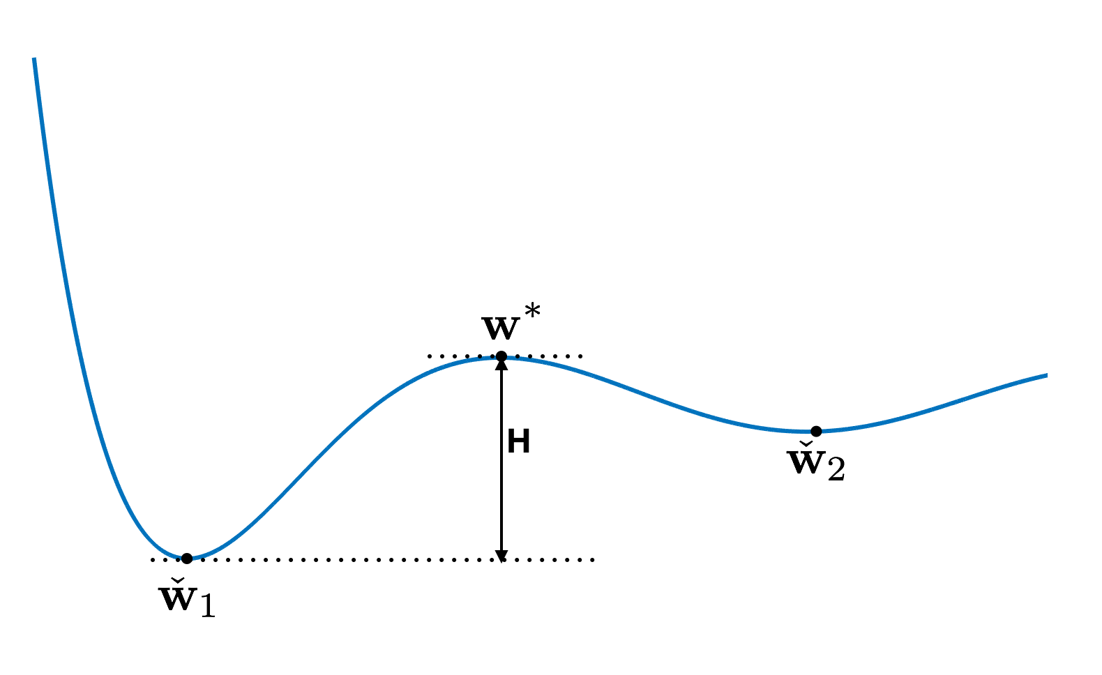
Figure 2: A sketch of two local minimizer 𝐰ˇ1subscriptˇ𝐰1\check{\mathbf{w}}_{1} and 𝐰ˇ2subscriptˇ𝐰2\check{\mathbf{w}}_{2} of a risk function. The 𝐰superscript𝐰\mathbf{w}^{*} is the saddle point between 𝐰ˇ1subscriptˇ𝐰1\check{\mathbf{w}}_{1} and 𝐰ˇ2subscriptˇ𝐰2\check{\mathbf{w}}_{2} and the H𝐻H is the relative height of 𝐰superscript𝐰\mathbf{w}^{*} to 𝐰ˇ1subscriptˇ𝐰1\check{\mathbf{w}}_{1}.

We first consider the behavior of SGD in the finite-time regime t<𝑡t<\infty, which is typical in the practice. Specifically, we are interested in the escape time of SGD from one local minimizer 𝐰ˇ1subscriptˇ𝐰1\check{\mathbf{w}}_{1} to its nearest local minimizer 𝐰ˇ2subscriptˇ𝐰2\check{\mathbf{w}}_{2}. Refer to the Figure 2 as an illustration. Let 𝐰superscript𝐰\mathbf{w}^{*} be the saddle point222There are possibly multiple saddle points between 𝐰ˇ1subscriptˇ𝐰1\check{\mathbf{w}}_{1} and 𝐰ˇ2subscriptˇ𝐰2\check{\mathbf{w}}_{2}. We define 𝐰superscript𝐰\mathbf{w}^{*} as the saddle point with the minimal height among all saddle points in the following sense. Let w(t),0t1,𝑤𝑡0𝑡1w(t),0\leq t\leq 1, be any continuous path from 𝐰ˇ1subscriptˇ𝐰1\check{\mathbf{w}}_{1} to 𝐰ˇ2subscriptˇ𝐰2\check{\mathbf{w}}_{2}. Denote by w^=arginfw:w(0)=𝐰ˇ1,w(1)=𝐰ˇ2supt[0,1]L(w(t))^𝑤subscriptinf:𝑤formulae-sequence𝑤0subscriptˇ𝐰1𝑤1subscriptˇ𝐰2subscriptsupremum𝑡01𝐿𝑤𝑡\widehat{w}=\arg{\text{inf}}_{w:w(0)=\check{\mathbf{w}}_{1},w(1)=\check{\mathbf{w}}_{2}}\sup_{t\in[0,1]}L(w(t)) the path with the minimal saddle point height among all continuous path. We define that 𝐰=maxt[0,1]w^(t)superscript𝐰subscript𝑡01^𝑤𝑡\mathbf{w}^{*}=\max_{t\in[0,1]}\widehat{w}(t). between 𝐰ˇ1subscriptˇ𝐰1\check{\mathbf{w}}_{1} and 𝐰ˇ2subscriptˇ𝐰2\check{\mathbf{w}}_{2}. By the definition of 𝐰superscript𝐰\mathbf{w}^{*}, the Hessian ΔL(𝐰)Δ𝐿superscript𝐰\Delta L(\mathbf{w}^{*}) can be shown to have a single negative eigenvalue λsuperscript𝜆-\lambda^{*} (e.g., Berglund (2013)). By the Eyring-Kramers formula, we have the following theorem.

Theorem 2.2.

Let τ𝐰ˇ1𝐰ˇ2subscript𝜏subscriptˇ𝐰1subscriptˇ𝐰2\tau_{\check{\mathbf{w}}_{1}\to\check{\mathbf{w}}_{2}} be the transition time from 𝐰ˇ1subscriptˇ𝐰1\check{\mathbf{w}}_{1} to 𝐰ˇ2subscriptˇ𝐰2\check{\mathbf{w}}_{2} for 𝐖(t)𝐖𝑡\mathbf{W}(t), then

𝔼[τ𝐰ˇ1𝐰ˇ2]=2πλ|ΔL(𝐰)||ΔL(𝐰ˇ1)|eH2M(𝐰ˇ1)/[γ(𝐰ˇ1)β(𝐰ˇ1)]{1+O(ϵlog(ϵ1))}𝔼delimited-[]subscript𝜏subscriptˇ𝐰1subscriptˇ𝐰22𝜋superscript𝜆Δ𝐿superscript𝐰Δ𝐿subscriptˇ𝐰1superscript𝑒𝐻2𝑀subscriptˇ𝐰1delimited-[]𝛾subscriptˇ𝐰1𝛽subscriptˇ𝐰11𝑂italic-ϵsuperscriptitalic-ϵ1\mathbb{E}[\tau_{\check{\mathbf{w}}_{1}\to\check{\mathbf{w}}_{2}}]=\frac{2\pi}{\lambda^{*}}\sqrt{\frac{|\Delta L(\mathbf{w}^{*})|}{|\Delta L(\check{\bf{w}}_{1})|}}e^{H\cdot 2M(\check{\mathbf{w}}_{1})/[\gamma(\check{\mathbf{w}}_{1})\beta(\check{\mathbf{w}}_{1})]}\{1+O\left(\sqrt{\epsilon}\log(\epsilon^{-1})\right)\}

where |ΔL()|Δ𝐿|\Delta L(\cdot)| represents for the determinate of the Hessian, H=H(𝐰,𝐰ˇ1)L(𝐰)L(𝐰ˇ1)𝐻𝐻superscript𝐰subscriptˇ𝐰1𝐿superscript𝐰𝐿subscriptˇ𝐰1H=H(\mathbf{w}^{*},\check{\mathbf{w}}_{1})\equiv L(\mathbf{w}^{*})-L(\check{\mathbf{w}}_{1}) is the relative height of 𝐰superscript𝐰\mathbf{w}^{*} to 𝐰ˇ1subscriptˇ𝐰1\check{\mathbf{w}}_{1}, M(𝐰ˇ1)𝑀subscriptˇ𝐰1M(\check{\mathbf{w}}_{1}) is the batch size of the SGD at 𝐰ˇ1subscriptˇ𝐰1\check{\mathbf{w}}_{1}, γ(𝐰ˇ1)𝛾subscriptˇ𝐰1\gamma(\check{\mathbf{w}}_{1}) is the learning rate of the SGD at 𝐰ˇ1subscriptˇ𝐰1\check{\mathbf{w}}_{1}, and β𝛽\beta is defined in (2.4).

The above theorem is proved by Bovier et al. (2004, 2005) and in a more general case by Berglund (2013). From this theorem, one can see that the transition time depends on three factors, the diffusion factor γβ/M𝛾𝛽𝑀\gamma\beta/M in the SGD, the potential barrier H(𝐰,𝐰ˇ1)𝐻superscript𝐰subscriptˇ𝐰1H(\mathbf{w}^{*},\check{\mathbf{w}}_{1}) that SGD has to climb in order to escape 𝐰ˇ1subscriptˇ𝐰1\check{\mathbf{w}}_{1}, and the determinant of the Hessian at 𝐰ˇ1subscriptˇ𝐰1\check{\mathbf{w}}_{1} and 𝐰superscript𝐰\mathbf{w}^{*}.

The results shown in this Section 2.2 can explain the KMNST hypothesis as follows. A larger batch size M𝑀M of SGD at local minimizer 𝐰ˇ1subscriptˇ𝐰1\check{\mathbf{w}}_{1} corresponds to a longer escaping time from 𝐰ˇ1subscriptˇ𝐰1\check{\mathbf{w}}_{1}, which is modeled by 𝔼[τ𝐰ˇ1𝐰ˇ2]𝔼delimited-[]subscript𝜏subscriptˇ𝐰1subscriptˇ𝐰2\mathbb{E}[\tau_{\check{\mathbf{w}}_{1}\to\check{\mathbf{w}}_{2}}]. Hence, even if 𝐰ˇ1subscriptˇ𝐰1\check{\mathbf{w}}_{1} corresponds to a sharp minimum with a large |ΔL(𝐰ˇ1)|Δ𝐿subscriptˇ𝐰1|\Delta L(\check{\bf{w}}_{1})|, the exponential term exp[H2M(𝐰ˇ1)/[γ(𝐰ˇ1)β(𝐰ˇ1)]]𝐻2𝑀subscriptˇ𝐰1delimited-[]𝛾subscriptˇ𝐰1𝛽subscriptˇ𝐰1\exp[H\cdot 2M(\check{\mathbf{w}}_{1})/[\gamma(\check{\mathbf{w}}_{1})\beta(\check{\mathbf{w}}_{1})]] could dominate the escaping time. As a result, the large batch training will be trapped at a sharp minimizer in the finite-time regime, which is the same as observed by Keskar et al. (2017) that large batch training tends to converge to the sharp minimizer of the training function. On the other hand, if the batch size is small, then exp[H2M(𝐰ˇ1)/[γ(𝐰ˇ1)β(𝐰ˇ1)]]𝐻2𝑀subscriptˇ𝐰1delimited-[]𝛾subscriptˇ𝐰1𝛽subscriptˇ𝐰1\exp[H\cdot 2M(\check{\mathbf{w}}_{1})/[\gamma(\check{\mathbf{w}}_{1})\beta(\check{\mathbf{w}}_{1})]] is small. As a result, only when |ΔL(𝐰ˇ1)|Δ𝐿subscriptˇ𝐰1|\Delta L(\check{\mathbf{w}}_{1})| is small enough, then SGD can be trapped at this minimizer, which implies that small batch training tends to converge to flatter minima.

However, these phenomena will change in the asymptotic regime t𝑡t\to\infty as explained in Section 2.3.

2.3 KMNST hypothesis in the asymptotic regime

Main assumptions

In this section, we consider the asymptotic regime that t𝑡t\to\infty and suppose the following three assumptions333We note that if the parameter vector 𝐰𝐰\mathbf{w} lies in a bounded region, then the Gibbs density is well defined only if eL(𝐰)𝑑𝐰<superscript𝑒𝐿𝐰differential-d𝐰\int e^{-L(\mathbf{w})}d\mathbf{w}<\infty, the Poincaré inequality is always true, and the assumption (A.3) is always true. Thus, although the mean cross entropy loss with bounded parameters does not satisfy (A.1) or (A.2), our results in this section still hold for the mean cross entropy loss.:

  • (A.1)

    L(𝐰)𝐿𝐰L(\mathbf{w}) is confinement: lim𝐰+L(𝐰)=+subscriptnorm𝐰𝐿𝐰\lim_{\|\mathbf{w}\|\to+\infty}L(\mathbf{w})=+\infty and eL(𝐰)𝑑𝐰<+superscript𝑒𝐿𝐰differential-d𝐰\int e^{-L(\mathbf{w})}d\mathbf{w}<+\infty.

  • (A.2)

    lim𝐰+{L(𝐰)2/2L(𝐰)}=+subscriptnorm𝐰superscriptnorm𝐿𝐰22𝐿𝐰\lim_{\|\mathbf{w}\|\to+\infty}\left\{\|\nabla L(\mathbf{w})\|^{2}/2-\nabla\cdot\nabla L(\mathbf{w})\right\}=+\infty, where L𝐿\nabla\cdot\nabla L denotes the trace of the Hessian for L𝐿L. Moreover, lim𝐰+{L(𝐰)/L(𝐰)2}=0subscriptnorm𝐰𝐿𝐰superscriptnorm𝐿𝐰20\lim_{\|\mathbf{w}\|\to+\infty}\left\{\nabla\cdot\nabla L(\mathbf{w})/\|\nabla L(\mathbf{w})\|^{2}\right\}=0.

  • (A.3)

    There exists a constant M𝑀M, such that |eL(𝐰)(L(𝐰)2L(𝐰))|Msuperscript𝑒𝐿𝐰superscriptdelimited-∥∥𝐿𝐰2𝐿𝐰𝑀\left\lvert e^{-L(\mathbf{w})}\left(\left\lVert\nabla L(\mathbf{w})\right\rVert^{2}-\nabla\cdot\nabla L(\mathbf{w})\right)\right\rvert\leq M.

We show in Appendix C that (A.1) – (A.3) hold for typical loss functions such as the regularized mean cross entropy and the square loss functions. These assumptions appear commonly in the diffusion process literature, see, e.g., Pavliotis (2018). In particular, (A.1) ensures the Gibbs density function pG(𝐰)=eL(𝐰)subscript𝑝𝐺𝐰superscript𝑒𝐿𝐰p_{G}(\mathbf{w})=e^{-L(\mathbf{w})} is well defined, and (A.2) is sufficient for the measure μ(𝐰)=pG(𝐰)𝑑𝐰=eL(𝐰)𝑑𝐰𝜇𝐰subscript𝑝𝐺𝐰differential-d𝐰superscript𝑒𝐿𝐰differential-d𝐰\mu(\mathbf{w})=\int p_{G}(\mathbf{w})d\mathbf{w}=\int e^{-L(\mathbf{w})}d\mathbf{w} to satisfy the Poincaré inequality (e.g., Pavliotis (2018); Raginsky (2017)):

f(𝐰)2𝑑μ(𝐰)CP(f(𝐰)f(𝐰)𝑑μ(𝐰))2𝑑μ(𝐰), for some CP>0,formulae-sequencesuperscriptdelimited-∥∥𝑓𝐰2differential-d𝜇𝐰subscript𝐶𝑃superscript𝑓𝐰𝑓𝐰differential-d𝜇𝐰2differential-d𝜇𝐰 for some subscript𝐶𝑃0\displaystyle\int\left\lVert\nabla f(\mathbf{w})\right\rVert^{2}d\mu(\mathbf{w})\geq C_{P}\int\left(f(\mathbf{w})-\int f(\mathbf{w})d\mu(\mathbf{w})\right)^{2}d\mu(\mathbf{w}),\text{ for some }C_{P}>0, (2.6)

holds for any f𝑓f satisfying f2(𝐰)𝑑𝐰<superscript𝑓2𝐰differential-d𝐰\int f^{2}(\mathbf{w})d\mathbf{w}<\infty.

We first give the stationary solution for the Fokker-Planck equation (2.5) when t𝑡t\to\infty.

Lemma 2.3.

Under the assumption (A.1) and suppose β(𝐰)β𝛽𝐰𝛽\beta(\mathbf{w})\equiv\beta, then (2.5) has a stationary solution

p(𝐰)=κeηL(𝐰),subscript𝑝𝐰𝜅superscript𝑒subscript𝜂𝐿𝐰p_{\infty}(\mathbf{w})=\kappa e^{-\eta_{\infty}L(\mathbf{w})},

where

η=2M/[γβ(𝐰ˇ)]subscript𝜂2𝑀delimited-[]𝛾𝛽ˇ𝐰\eta_{\infty}=2M/[\gamma\beta(\check{\mathbf{w}})]

with the limiting batch size M=limtM(t)𝑀subscript𝑡𝑀𝑡M=\lim_{t\to\infty}M(t), the limiting learning rate γ=limtγ(t)𝛾subscript𝑡𝛾𝑡\gamma=\lim_{t\to\infty}\gamma(t), and the convergent local minimizer 𝐰ˇˇ𝐰\check{\mathbf{w}}. The constant κ𝜅\kappa in the above formula is a normalization factor such that p(𝐰)=1subscript𝑝𝐰1\int p_{\infty}(\mathbf{w})=1.

Proof for this lemma is given in Appendix D. We remark that for general β(𝐰)𝛽𝐰\beta(\mathbf{w}) depending on 𝐰𝐰\mathbf{w}, the existence and an explicit form of stationary solution for (2.5) remain an open question in the literature. Hence, we focus on β(𝐰)β𝛽𝐰𝛽\beta(\mathbf{w})\equiv\beta in this section.

Similar results as Lemma 2.3 can be found in related work, e.g., Jastrzebski et al. (2017). However, it is not clear whether p(𝐰,t)𝑝𝐰𝑡p(\mathbf{w},t) converges to p(𝐰)subscript𝑝𝐰p_{\infty}(\mathbf{w}), not to mention how fast that p(𝐰,t)𝑝𝐰𝑡p(\mathbf{w},t) would converge to p(𝐰)subscript𝑝𝐰p_{\infty}(\mathbf{w}). The following theorem gives a positive answer to this question, which later provides a new insight into the justification of KMNST hypothesis.

Theorem 2.4.

Under assumptions (A.1) – (A.3), the probability density function p(𝐰,t)𝑝𝐰𝑡p(\mathbf{w},t) of 𝐖(t)𝐖𝑡\mathbf{W}(t) converges to the stationary solution p(𝐰)subscript𝑝𝐰p_{\infty}(\mathbf{w}). Moreover, there exists T>0𝑇0T>0 such that for any t>T𝑡𝑇t>T,

p(𝐰,t)p(𝐰)p(𝐰)L2(d)2C(t,T)eCP(tT)/η,superscriptsubscriptdelimited-∥∥𝑝𝐰𝑡subscript𝑝𝐰subscript𝑝𝐰superscript𝐿2superscript𝑑2𝐶𝑡𝑇superscript𝑒subscript𝐶𝑃𝑡𝑇subscript𝜂\left\lVert\frac{p(\mathbf{w},t)-p_{\infty}(\mathbf{w})}{\sqrt{p_{\infty}(\mathbf{w})}}\right\rVert_{L^{2}(\mathbb{R}^{d})}^{2}\leq C(t,T)e^{-C_{P}\cdot(t-T)/\eta_{\infty}},

where CPsubscript𝐶𝑃C_{P} is a constant define in (2.6) and C(t,T)=CP(tT)/η+(p(T)p)/pL2(d)2𝐶𝑡𝑇subscript𝐶𝑃𝑡𝑇subscript𝜂superscriptsubscriptdelimited-∥∥𝑝𝑇subscript𝑝subscript𝑝superscript𝐿2superscript𝑑2C(t,T)=C_{P}\cdot(t-T)/\eta_{\infty}+\left\lVert({p(T)-p_{\infty}})/\sqrt{p_{\infty}}\right\rVert_{L^{2}(\mathbb{R}^{d})}^{2}.

The proof for this theorem is given in Appendix E. We also give a quantification of constant T𝑇T in Appendix F. Three remarks on Theorem 2.4 are as follows. First, this theorem shows that p(𝐰,t)𝑝𝐰𝑡p(\mathbf{w},t) always converges to psubscript𝑝p_{\infty} with an exponential rate regardless of the initial value. This theorem provides a theoretical ground for the work that manages to understand p(𝐰,t)𝑝𝐰𝑡p(\mathbf{w},t) based on analysis of the stationary distribution psubscript𝑝p_{\infty} (see, e.g., Jastrzebski et al. (2017)). Second, it is known (Raginsky, 2017) the Poincaré constant CPedproportional-tosubscript𝐶𝑃superscript𝑒𝑑C_{P}\propto e^{d}, where d𝑑d is the dimension of the parameter 𝐰𝐰\mathbf{w}. In the setting of the deep neural networks, CPsubscript𝐶𝑃C_{P} can be very large and it takes exponential time t>ed𝑡superscript𝑒𝑑t>e^{d} such that p(𝐰,t)𝑝𝐰𝑡p(\mathbf{w},t) would approach to the stationary distribution psubscript𝑝p_{\infty}. Therefore, the results only based on the stationary solution do not reveal information in the finite-time regime. Third, the convergence rate is relatively faster with a larger γ/M𝛾𝑀\gamma/M since it corresponds to a smaller ηsubscript𝜂\eta_{\infty}. The last two remarks are illustrated by experiments in Section 3.

We now characterize 𝐖(t)𝐖𝑡\mathbf{W}(t) in the asymptotic regime t𝑡t\to\infty based on the stationary distribution psubscript𝑝p_{\infty}, and we give the proof of the following theorem in Appendix G.

Theorem 2.5.

Let 𝐰ˇˇ𝐰\check{\mathbf{w}} be a local minimizer. Then,

limϵ0(|𝐖()𝐰ˇ|ϵ)=κe2ηL(𝐰ˇ)ηd/2|ΔL(𝐰ˇ)|limϵ0[eηϵ2j=1d1eϵ2ηλj/π],subscriptitalic-ϵ0𝐖ˇ𝐰italic-ϵ𝜅superscript𝑒2subscript𝜂𝐿ˇ𝐰superscriptsubscript𝜂𝑑2Δ𝐿ˇ𝐰subscriptitalic-ϵ0delimited-[]superscript𝑒subscript𝜂superscriptitalic-ϵ2superscriptsubscriptproduct𝑗1𝑑1superscript𝑒superscriptitalic-ϵ2subscript𝜂subscript𝜆𝑗𝜋\displaystyle\lim_{\epsilon\to 0}\mathbb{P}(|\mathbf{W}(\infty)-\check{\mathbf{w}}|\leq\epsilon)=\frac{\kappa e^{-2\eta_{\infty}L(\check{\mathbf{w}})}}{\eta_{\infty}^{d/2}\sqrt{|\mathrm{\Delta}L(\check{\mathbf{w}})|}}\lim_{\epsilon\to 0}\left[e^{\eta_{\infty}\epsilon^{2}}\prod_{j=1}^{d}\sqrt{1-e^{-\epsilon^{2}\eta_{\infty}\lambda_{j}/\pi}}\right],

where d𝑑d is the dimension of 𝐰𝐰\mathbf{w}, λjsubscript𝜆𝑗\lambda_{j}s and |ΔL(𝐰ˇ)|Δ𝐿ˇ𝐰|\mathrm{\Delta}L(\check{\mathbf{w}})| represent the eigenvalues and the determinant of loss function Hessian ΔL(𝐰ˇ)Δ𝐿ˇ𝐰\mathrm{\Delta}L(\check{\mathbf{w}}), respectively, and the constants κ,η𝜅subscript𝜂\kappa,\eta_{\infty} are defined in Lemma 2.3.

Given the complex form of the probability in Theorem 2.5, we give numerical illustrations in Appendix H. To appreciate the implication of Theorem 2.5, we consider any two local minimizers 𝐰ˇ1subscriptˇ𝐰1\check{\mathbf{w}}_{1} and 𝐰ˇ2subscriptˇ𝐰2\check{\mathbf{w}}_{2} with the same value of L(𝐰ˇ1)=L(𝐰ˇ2)𝐿subscriptˇ𝐰1𝐿subscriptˇ𝐰2L(\check{\mathbf{w}}_{1})=L(\check{\mathbf{w}}_{2}). Then,

limϵ0(|𝐖()𝐰ˇ1|ϵ)(|𝐖()𝐰ˇ2|ϵ)=|ΔL(𝐰ˇ2)||ΔL(𝐰ˇ1)|.subscriptitalic-ϵ0𝐖subscriptˇ𝐰1italic-ϵ𝐖subscriptˇ𝐰2italic-ϵΔ𝐿subscriptˇ𝐰2Δ𝐿subscriptˇ𝐰1\displaystyle\lim_{\epsilon\to 0}\frac{\mathbb{P}(|\mathbf{W}(\infty)-\check{\mathbf{w}}_{1}|\leq\epsilon)}{\mathbb{P}(|\mathbf{W}(\infty)-\check{\mathbf{w}}_{2}|\leq\epsilon)}=\sqrt{\frac{\left\lvert\Delta L(\check{\mathbf{w}}_{2})\right\rvert}{\left\lvert\Delta L(\check{\mathbf{w}}_{1})\right\rvert}}. (2.7)

The ratio of probability (2.7) implies that in the asymptotic regime t𝑡t\to\infty, the probability of SGD converging to a flatter minimum with a smaller determinant |ΔL()|Δ𝐿|\Delta L(\cdot)| is always larger than the probability of SGD converging to a sharper minimum with a larger determinant |ΔL()|Δ𝐿|\Delta L(\cdot)|. Moreover, (2.7) does not depend on the batch size or learning rate, but it only depends on the determinant of Hessian at the local minimum.

The results derived in this Section 2.3 provide some new insights into the KMNST hypothesis: SGD tends to converge to flatter minima regardless of the batch size M𝑀M (or the ratio γ/M𝛾𝑀\gamma/M) in the asymptotic regime t𝑡t\to\infty as shown by (2.7). However, it may take exponential time edsuperscript𝑒𝑑e^{d} to converge, where d𝑑d is the dimension of the model parameter 𝐰𝐰\mathbf{w}. The experiments in Section 3 further corroborate these theoretical finding.

3 Numerical Experiments

In this section, we show experiments to corroborate the theoretical findings in the previous section. We train 4-layer batch-normalized ReLU MLPs on MNIST with different learning rate γ𝛾\gamma and batch size M𝑀M. Specifically, we use three γ/M𝛾𝑀\gamma/M ratios: γ/M=0.01/128,0.1/128,0.2/256𝛾𝑀0.011280.11280.2256\gamma/M=0.01/128,0.1/128,0.2/256. As is common for such tasks, the mean cross entropy loss is used as the loss function. We discussed in Section 2.1 that this loss satisfies our assumptions for theoretical analysis.
Refer to caption
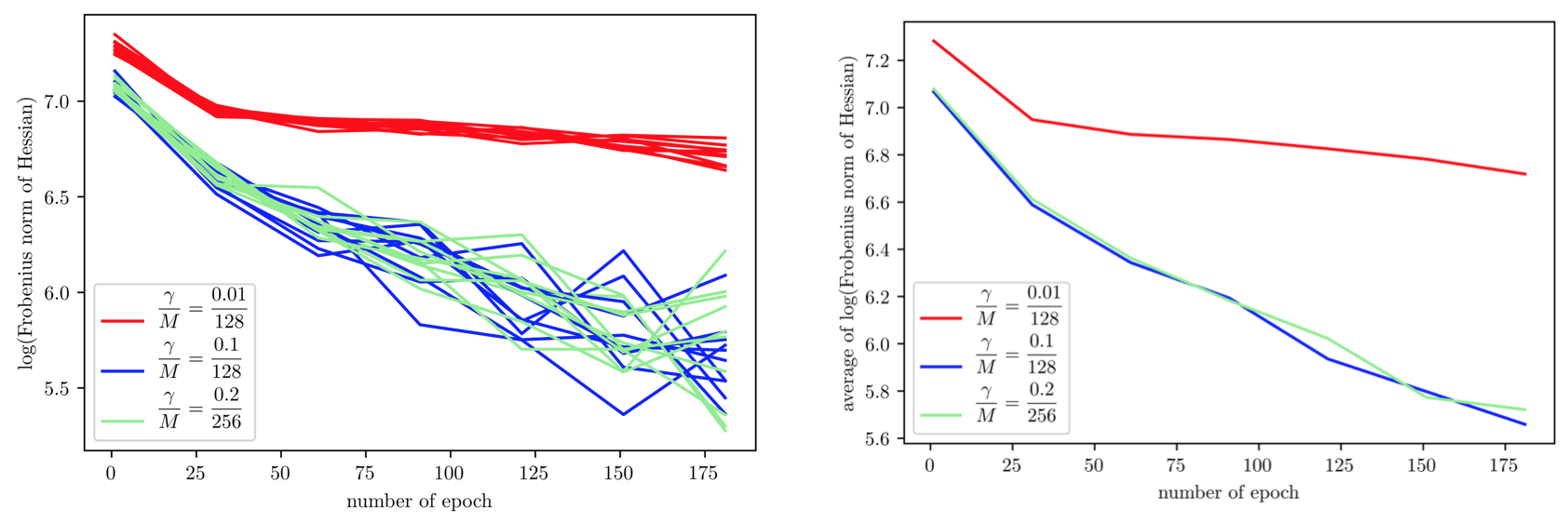
Figure 3: Log of Frobenius norm of Hessian as a function of epochs. Three (γ,M)𝛾𝑀(\gamma,M) pairs (0.01,128)0.01128(0.01,128), (0.1,128)0.1128(0.1,128) and (0.2,256)0.2256(0.2,256) are studied, which are denoted in red, blue and green, respectively. The left plot shows 10 experiments for each of three (γ,M)𝛾𝑀(\gamma,M) pairs and the right plot shows the average of 10 experiments. Total 180 epochs are trained.

Geometry of SGD updates

Figure 3 shows the log of Frobenius norm of Hessian for minima obtained by SGD. Due to the high computational cost for computing the determinant of the Hessian, we use the Frobenius norm of the Hessian as a substitute. Note that a larger Frobenius norm of Hessian corresponds to a sharper minimum. The Frobenius norm is approximated using the method in Wu and Zhu (2017). Note that the dynamics of SGD behave similar across 10 experiments for each of three γ/M𝛾𝑀\gamma/M ratios as shown in the left plot of Figure 3. Hence we focus on the averaged dynamics as in the right plot of Figure 3. Three main results can be observed from Figure 3:

  • First, for the same γ/M𝛾𝑀\gamma/M ratio (e.g., γ/M=0.1/128𝛾𝑀0.1128\gamma/M=0.1/128 and 0.2/2560.22560.2/256), the minima obtained by SGD have the very similar norm of the Hessian. This illustrates the Lemma 2.1, 2.3 and Theorem 2.2 that the dynamics and geometry of the minima obtained by SGD would depend on the ratio γ/M𝛾𝑀\gamma/M instead of individual γ𝛾\gamma or M𝑀M separately. A similar phenomenon is also observed by Jastrzebski et al. (2017).

  • Second, since the SGD is trained using 180 epochs, the dynamics of SGD in Figure 3 fall in the finite-time regime. It is clear that the rate of SGD tending to a flatter minimum (i.e., with a smaller norm of the Hessian) with a larger γ/M𝛾𝑀\gamma/M ratio (e.g., γ/M=0.1/128𝛾𝑀0.1128\gamma/M=0.1/128) is faster compared to with a smaller γ/M𝛾𝑀\gamma/M ratio (e.g., γ/M=0.01/128𝛾𝑀0.01128\gamma/M=0.01/128). This illustrates the finite-time analysis in Theorem 2.2 that the SGD with a smaller γ/M𝛾𝑀\gamma/M ratio is easier to be trapped around a minimum and hence the SGD tends to other minima slower. As a result, the Hessian of minima changes slower for SGD with a smaller γ/M𝛾𝑀\gamma/M ratio.

  • Third, Figure 3 also sheds light on the dynamics of SGD in the asymptotic regime. The SGD tends to converge to a flatter minimum regardless of the γ/M𝛾𝑀\gamma/M ratio, which demonstrates Theorem 2.5 and its corollary (2.7). However, the convergence rate is slow, in particular for the SGD with a small γ/M𝛾𝑀\gamma/M ratio, which is theoretically shown in Theorem 2.4 and its following remarks.

Training and generalization of SGD

Refer to caption
Figure 4: The left plot shows the training accuracy as a function of epochs and the right plot shows the cross entropy loss as a function of epochs. Three (γ,M)𝛾𝑀(\gamma,M) pairs (0.01,128)0.01128(0.01,128), (0.1,128)0.1128(0.1,128) and (0.2,256)0.2256(0.2,256) are studied, which are denoted in red, blue and green, respectively. Both plots show 10 experiments for each of three (γ,M)𝛾𝑀(\gamma,M) pairs. Total 180 epochs are trained.
Refer to caption
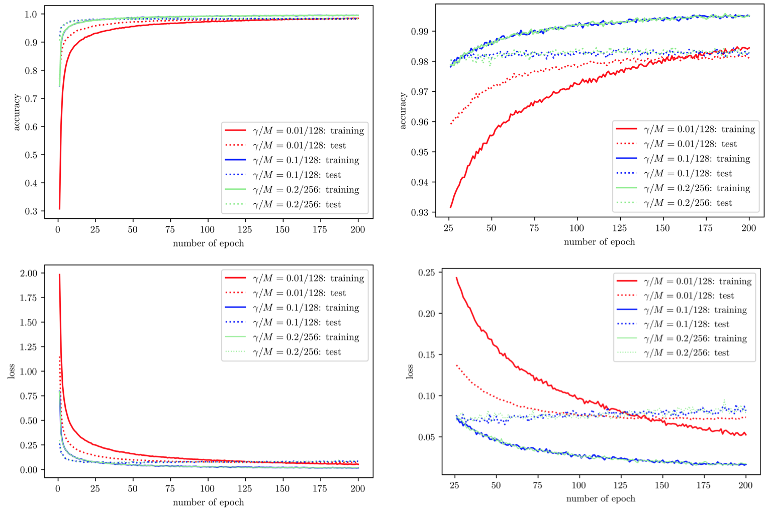
Figure 5: The top left plot shows the training and test accuracy as a function of epochs. The top right plot gives the zoomed in performance of the accuracy when epochs are no less than 25. The bottom left plot shows the cross entropy loss as a function of epochs. The bottom right plot gives the zoomed in performance of the loss when epochs are no less than 25. Three (γ,M)𝛾𝑀(\gamma,M) pairs (0.01,128)0.01128(0.01,128), (0.1,128)0.1128(0.1,128) and (0.2,256)0.2256(0.2,256) are studied, which are denoted in red, blue and green, respectively. Total 200 epochs are trained.

Figure 4 shows the training accuracy and loss for the model trained by SGD. We run 10 experiments. It is clear that the training accuracy and loss are very close across 10 experiments for each of three γ/M𝛾𝑀\gamma/M ratios. Thus, we focus on interpreting the training and generalization performance of the model obtain from one experiment, which is shown in Figure 5. Three main results can be observed from Figure 5:

  • First, for the same γ/M𝛾𝑀\gamma/M ratio (e.g., γ/M=0.1/128𝛾𝑀0.1128\gamma/M=0.1/128 and 0.2/2560.22560.2/256), the training error and test error are very close. This meets our expectation since the dynamics of SGD only depends on the ratio γ/M𝛾𝑀\gamma/M as discussed above and the models trained by SGD with the same γ/M𝛾𝑀\gamma/M ratio should behave similarly.

  • Second, the model obtained with a larger γ/M𝛾𝑀\gamma/M ratio (e.g., γ/M=0.1/128𝛾𝑀0.1128\gamma/M=0.1/128) gives a better training accuracy and a smaller training loss compared with the case of a smaller γ/M𝛾𝑀\gamma/M ratio (e.g., γ/M=0.01/128𝛾𝑀0.01128\gamma/M=0.01/128). This can be partially justified by our finite-time analysis in Theorem 2.2 that the SGD with a larger γ/M𝛾𝑀\gamma/M ratio is easier to escape a local minimum.

  • Third, the model obtained with a smaller γ/M𝛾𝑀\gamma/M ratio gives a smaller test loss after a certain time (it is after 100 epochs in the bottom right plot of Figure 5). This can be explained by Lemma 2.1 and its following remark. Specifically, a smaller γ/M𝛾𝑀\gamma/M ratio corresponds a mean drift deviates less from the mean drift L(𝐰)𝐿𝐰-\nabla L(\mathbf{w}), where L(𝐰)𝐿𝐰-\nabla L(\mathbf{w}) is the drift for a global minimizer of the risk function L(𝐰)𝐿𝐰L(\mathbf{w}). This shows a tradeoff between the large and small γ/M𝛾𝑀\gamma/M ratio in the sense of the training and test loss.

4 Related work

The modeling of SDE for approximating SGD is well studied in the literature. See, e.g., Mandt et al. (2017); Poggio (2017); Li et al. (2017); Jastrzebski et al. (2017); Chaudhari et al. (2017) and the references therein. Different from these work, we give a new result in Lemma 2.1, which not only gives the dynamics of SDE solution but also connects with the generalization performance. We also derive the theory for the SDE solution in the asymptotic regime, especially the convergence rate.

We clarify the definition of the sharpness in multi-dimensional cases. We find that the production of eigenvalues, or equivalently, the determinant of the risk function Hessian at minimizers is appropriate. Similar results have been derived in Jastrzebski et al. (2017); Dziugaite and Roy (2017).

The work by Jastrzebski et al. (2017) remarkably emphasize how the learning rate to batch size ratio affects the SGD and they also relate with the KMNST hypothesis. Here are some differences between Jastrzebski et al. (2017) and ours.

  • Jastrzebski et al. (2017) use the stationary probability p(𝐰)subscript𝑝𝐰p_{\infty}(\mathbf{w}) to explain that the behavior of the SGD. However, we show that it takes the exponential time for p(𝐰,t)𝑝𝐰𝑡p(\mathbf{w},t) to converge to p(𝐰)subscript𝑝𝐰p_{\infty}(\mathbf{w}) in the setting of the deep neural network. Hence, p(𝐰)subscript𝑝𝐰p_{\infty}(\mathbf{w}) cannot fully explain the behavior of SGD in the practical finite-time regime. Our work adds new elements to this picture by studying the escaping time of SGD from a local minimum in the sense of finite-time regime and we also give a new result on the convergence rate of p(𝐰,t)p(𝐰)𝑝𝐰𝑡subscript𝑝𝐰p(\mathbf{w},t)\to p_{\infty}(\mathbf{w}).

  • In particular, the stationary probability in Jastrzebski et al. (2017) can not explain the KMNST hypothesis when two local minimizers 𝐰ˇ1subscriptˇ𝐰1\check{\mathbf{w}}_{1} and 𝐰ˇ2subscriptˇ𝐰2\check{\mathbf{w}}_{2} having a same risk L(𝐰ˇ1)=L(𝐰ˇ2)𝐿subscriptˇ𝐰1𝐿subscriptˇ𝐰2L(\check{\mathbf{w}}_{1})=L(\check{\mathbf{w}}_{2}). In this case, the result of Jastrzebski et al. (2017) coincides with (2.7) and it is independent of M𝑀M or γ𝛾\gamma, which is undesired in explaining the KMNST hypothesis. On the other hand, there may exist many minima with a same risk value but different Hessians for a deep neural network. Therefore, our finite-time results can give a better explanation to the KMNST hypothesis in this case.

5 Conclusion

In this paper, we investigate the relationship between the sharpness of the minima that SGD converges to with the ratio of the step size and the batch size. Using the SDE as the approximation of SGD, we explain part of the hypothesis proposed by Keskar et al. (2017) that large-batch methods tend to converge to sharp minimizers of the training function using the escaping time theorem in the finite-time regime. We prove that for the isotropic case the probability density function of SGD will converge to the stationary solution for any initial data regardless of the time varying step size and batch size. We give the convergence rate, which indicates that with a larger ratio of the learning rate and the batch size, the probability will converge faster to the stationary solution. Asymptotically the probability of converging to the global minimum is independent of the batch size and learning rate, but it only depends on the sharpness of the minimum. We verify these theoretical findings with numerical experiments.

There are many directions for further study such as how the ratio of the step size and batch size influence the generalization error. In our experiment, it indicates that with a larger learning rate to batch size ratio the generalization error is worse. Further theoretical analysis is desired. Another interesting topic is to study the stationary solution and the evolution the probability density function of SGD when the variance matrix is anisotropic, which remain open questions.

Appendix

Appendix A Proof of (2.2)

For the first part, without less of generality, we consider 𝐰𝐰\mathbf{w} is in any bounded domain of \mathbb{R}. Then

L(𝐰)=dd𝐰𝔼[Ln(𝐰)]𝐿𝐰𝑑𝑑𝐰𝔼delimited-[]subscript𝐿𝑛𝐰\displaystyle\nabla L(\mathbf{w})=\frac{d}{d\mathbf{w}}\mathbb{E}[L_{n}(\mathbf{w})] =limh01h{𝔼[Ln(𝐰+h)]𝔼[Ln(𝐰)]}absentsubscript01𝔼delimited-[]subscript𝐿𝑛𝐰𝔼delimited-[]subscript𝐿𝑛𝐰\displaystyle=\lim_{h\to 0}\frac{1}{h}\left\{\mathbb{E}[L_{n}(\mathbf{w}+h)]-\mathbb{E}[L_{n}(\mathbf{w})]\right\}
=limh0𝔼{Ln(𝐰+h)Ln(𝐰)h}=limh0𝔼{Ln(𝐰+τ(h))}.absentsubscript0𝔼subscript𝐿𝑛𝐰subscript𝐿𝑛𝐰subscript0𝔼subscript𝐿𝑛𝐰𝜏\displaystyle=\lim_{h\to 0}\mathbb{E}\left\{\frac{L_{n}(\mathbf{w}+h)-L_{n}(\mathbf{w})}{h}\right\}=\lim_{h\to 0}\mathbb{E}\left\{\nabla L_{n}(\mathbf{w}+\tau(h))\right\}.

where the last step is by the mean value theorem with some 0<τ(h)<h0𝜏0<\tau(h)<h. Due to continuity of Lnsubscript𝐿𝑛\nabla L_{n}, we can use the dominated convergence theorem and have

limh0𝔼{Ln(𝐰+τ(h))}=𝔼{limh0Ln(𝐰+τ(h))}=𝔼{Ln(𝐰)}.subscript0𝔼subscript𝐿𝑛𝐰𝜏𝔼subscript0subscript𝐿𝑛𝐰𝜏𝔼subscript𝐿𝑛𝐰\lim_{h\to 0}\mathbb{E}\left\{\nabla L_{n}(\mathbf{w}+\tau(h))\right\}=\mathbb{E}\left\{\lim_{h\to 0}\nabla L_{n}(\mathbf{w}+\tau(h))\right\}=\mathbb{E}\left\{\nabla L_{n}(\mathbf{w})\right\}.

This completes the proof of the first part. By assuming the iid of the data, we have Var[𝐠^(B)]=M1𝝈2(𝐰)Vardelimited-[]superscript^𝐠𝐵superscript𝑀1superscript𝝈2𝐰\text{Var}[\widehat{\mathbf{g}}^{(B)}]=M^{-1}\bm{\sigma}^{2}(\mathbf{w}). This completes the proof of the second part.

Appendix B Proof of Lemma 2.1

We start to consider when β(𝐰)β𝛽𝐰𝛽\beta(\mathbf{w})\equiv\beta is a constant and follow the strategy in Kolpas. et al. (2007) to derive the Fokker-Planck equation. First, consider 𝐖(t)=W(t)𝐖𝑡𝑊𝑡\mathbf{W}(t)=W(t)\in\mathbb{R}. Note that for SGD the corresponding W(t)𝑊𝑡W(t) is a Markov process, then the Chapman-Kolmogorov equation gives

p(W(t3)|W(t1))=+p(W(t3)|W(t2)=w)p(W(t2)=w|W(t1))𝑑w.𝑝conditional𝑊subscript𝑡3𝑊subscript𝑡1superscriptsubscript𝑝conditional𝑊subscript𝑡3𝑊subscript𝑡2𝑤𝑝𝑊subscript𝑡2conditional𝑤𝑊subscript𝑡1differential-d𝑤p\left(W(t_{3})|W(t_{1})\right)=\int_{-\infty}^{+\infty}p\left(W(t_{3})|W(t_{2})=w\right)p\left(W(t_{2})=w|W(t_{1})\right)dw.

Consider the integral

I=+h(w)tp(w,t|W)dw,𝐼superscriptsubscript𝑤subscript𝑡𝑝𝑤conditional𝑡𝑊𝑑𝑤I=\int_{-\infty}^{+\infty}h(w)\partial_{t}p(w,t|W)dw,

where h(w)𝑤h(w) is a smooth function with compact support. Observe that

+h(w)tp(w,t|W)dw=limΔt0+h(w)(p(w,t+Δt|W)p(w,t|W)Δt)𝑑w.superscriptsubscript𝑤subscript𝑡𝑝𝑤conditional𝑡𝑊𝑑𝑤subscriptΔ𝑡0superscriptsubscript𝑤𝑝𝑤𝑡conditionalΔ𝑡𝑊𝑝𝑤conditional𝑡𝑊Δ𝑡differential-d𝑤\int_{-\infty}^{+\infty}h(w)\partial_{t}p(w,t|W)dw=\lim_{\Delta t\to 0}\int_{-\infty}^{+\infty}h(w)\left(\frac{p(w,t+\Delta t|W)-p(w,t|W)}{\Delta t}\right)dw.

Letting Z𝑍Z be an intermediate point. Applying the Chapman-Kolmogorov identity on the right hand side yields

limΔt01Δt(+h(w)+p(w,Δt|Z)p(Z,t|W)𝑑Z𝑑w+h(w)p(w,t|W)𝑑w).subscriptΔ𝑡01Δ𝑡superscriptsubscript𝑤superscriptsubscript𝑝𝑤conditionalΔ𝑡𝑍𝑝𝑍conditional𝑡𝑊differential-d𝑍differential-d𝑤superscriptsubscript𝑤𝑝𝑤conditional𝑡𝑊differential-d𝑤\lim_{\Delta t\to 0}\frac{1}{\Delta t}\left(\int_{-\infty}^{+\infty}h(w)\int_{-\infty}^{+\infty}p(w,\Delta t|Z)p(Z,t|W)dZdw-\int_{-\infty}^{+\infty}h(w)p(w,t|W)dw\right).

By changing the limits of integration in the first term and letting w𝑤w approach Z𝑍Z in the second term, we obtain

limΔt01Δt(+p(Z,t|W)+p(w,Δt|Z)(h(w)h(Z))𝑑w𝑑Z).subscriptΔ𝑡01Δ𝑡superscriptsubscript𝑝𝑍conditional𝑡𝑊superscriptsubscript𝑝𝑤conditionalΔ𝑡𝑍𝑤𝑍differential-d𝑤differential-d𝑍\lim_{\Delta t\to 0}\frac{1}{\Delta t}\left(\int_{-\infty}^{+\infty}p(Z,t|W)\int_{-\infty}^{+\infty}p(w,\Delta t|Z)(h(w)-h(Z))dwdZ\right).

Expand h(w)𝑤h(w) as a Taylor series about Z𝑍Z, we can write the above integral as

limΔt01Δt(+p(Z,t|W)+p(w,Δt|Z)n=1h(n)(Z)(wZ)nn!)dwdZ.subscriptΔ𝑡01Δ𝑡superscriptsubscript𝑝𝑍conditional𝑡𝑊superscriptsubscript𝑝𝑤conditionalΔ𝑡𝑍superscriptsubscript𝑛1superscript𝑛𝑍superscript𝑤𝑍𝑛𝑛𝑑𝑤𝑑𝑍\lim_{\Delta t\to 0}\frac{1}{\Delta t}\left(\int_{-\infty}^{+\infty}p(Z,t|W)\int_{-\infty}^{+\infty}p(w,\Delta t|Z)\sum_{n=1}^{\infty}h^{(n)}(Z)\frac{(w-Z)^{n}}{n!}\right)dwdZ.

Now we define the function

D(n)(Z)=1n!1Δt+p(w,Δt|Z)(wZ)n𝑑w.superscript𝐷𝑛𝑍1𝑛1Δ𝑡superscriptsubscript𝑝𝑤conditionalΔ𝑡𝑍superscript𝑤𝑍𝑛differential-d𝑤D^{(n)}(Z)=\frac{1}{n!}\frac{1}{\Delta t}\int_{-\infty}^{+\infty}p(w,\Delta t|Z)(w-Z)^{n}dw.

We can write the integral I𝐼I as

+h(w)tp(w,t|W)dw=+p(Z,t|W)n=1D(n)(Z)h(n)(Z)dZ.superscriptsubscript𝑤subscript𝑡𝑝𝑤conditional𝑡𝑊𝑑𝑤superscriptsubscript𝑝𝑍conditional𝑡𝑊superscriptsubscript𝑛1superscript𝐷𝑛𝑍superscript𝑛𝑍𝑑𝑍\int_{-\infty}^{+\infty}h(w)\partial_{t}p(w,t|W)dw=\int_{-\infty}^{+\infty}p(Z,t|W)\sum_{n=1}^{\infty}D^{(n)}(Z)h^{(n)}(Z)dZ.

Integrating by parts n𝑛n times gives

tp(w,t)=n=1nZn[D(n)(Z)p(Z,t|W)].subscript𝑡𝑝𝑤𝑡superscriptsubscript𝑛1superscript𝑛superscript𝑍𝑛delimited-[]superscript𝐷𝑛𝑍𝑝𝑍conditional𝑡𝑊\partial_{t}p(w,t)=\sum_{n=1}^{\infty}-\frac{\partial^{n}}{\partial Z^{n}}\left[D^{(n)}(Z)p(Z,t|W)\right].

Let D(1)(w)=L(w)superscript𝐷1𝑤𝐿𝑤D^{(1)}(w)=-L(w), D(2)(w)=γ(t)β/[2M(t)]superscript𝐷2𝑤𝛾𝑡𝛽delimited-[]2𝑀𝑡D^{(2)}(w)=-\gamma(t)\beta/[2M(t)] and D(n)(w)=0superscript𝐷𝑛𝑤0D^{(n)}(w)=0 for all n3𝑛3n\geq 3, the above equation yields

tp(w,t)=w[L(w)p(w,t)]+w2[γ(t)β2M(t)p(w,t)],subscript𝑡𝑝𝑤𝑡𝑤delimited-[]𝐿𝑤𝑝𝑤𝑡superscript𝑤2delimited-[]𝛾𝑡𝛽2𝑀𝑡𝑝𝑤𝑡\partial_{t}p(w,t)=\frac{\partial}{\partial w}\left[\nabla L(w)p(w,t)\right]+\frac{\partial}{\partial w^{2}}\left[\frac{\gamma(t)\beta}{2M(t)}p(w,t)\right],

which is the Fokker-Planck equation in one variable. For the multidimensional case 𝐖=(W1,W2,,Wp)p𝐖subscript𝑊1subscript𝑊2subscript𝑊𝑝superscript𝑝\mathbf{W}=(W_{1},W_{2},\ldots,W_{p})\in\mathbb{R}^{p}, the above procedure can be easily generalized to get

tp(𝐰,t)subscript𝑡𝑝𝐰𝑡\displaystyle\partial_{t}p(\mathbf{w},t) =i=1pwi[L(𝐰)p(𝐰,t)]+i=1p2wi2[γ(t)β2M(t)p(𝐰,t)]absentsuperscriptsubscript𝑖1𝑝subscript𝑤𝑖delimited-[]𝐿𝐰𝑝𝐰𝑡superscriptsubscript𝑖1𝑝superscript2superscriptsubscript𝑤𝑖2delimited-[]𝛾𝑡𝛽2𝑀𝑡𝑝𝐰𝑡\displaystyle=\sum_{i=1}^{p}\frac{\partial}{\partial w_{i}}\left[\nabla L(\mathbf{w})p(\mathbf{w},t)\right]+\sum_{i=1}^{p}\frac{\partial^{2}}{\partial w_{i}^{2}}\left[\frac{\gamma(t)\beta}{2M(t)}p(\mathbf{w},t)\right] (B.1)
=(L(𝐰)p+γ(t)β2M(t)p).absent𝐿𝐰𝑝𝛾𝑡𝛽2𝑀𝑡𝑝\displaystyle=\nabla\cdot\left(\nabla L(\mathbf{w})p+\frac{\gamma(t)\beta}{2M(t)}\nabla p\right).

Since 𝐖(0)=𝐰0𝐖0subscript𝐰0\mathbf{W}(0)=\mathbf{w}_{0}, p(𝐰,0)=δ(𝐰0)𝑝𝐰0𝛿subscript𝐰0p(\mathbf{w},0)=\delta(\mathbf{w}_{0}). This completes the derivation of the Fokker-Planck equation for constant β(𝐰)=β𝛽𝐰𝛽\beta(\mathbf{w})=\beta. For deriving (2.5), we can apply (B.1) and notice that

[γ(t)β(𝐰)2M(t)p]=[γ(t)β(𝐰)2M(t)]p+γ(t)β(𝐰)2M(t)p.𝛾𝑡𝛽𝐰2𝑀𝑡𝑝𝛾𝑡𝛽𝐰2𝑀𝑡𝑝𝛾𝑡𝛽𝐰2𝑀𝑡𝑝\nabla\left[\frac{\gamma(t)\beta(\mathbf{w})}{2M(t)}p\right]=\nabla\left[\frac{\gamma(t)\beta(\mathbf{w})}{2M(t)}\right]p+\frac{\gamma(t)\beta(\mathbf{w})}{2M(t)}\nabla p.

This completes the proof.

Appendix C Discussion on the main assumptions (A.1) – (A.3).

We verify (A.1) and (A.2) for the L2subscript𝐿2L_{2} loss and the mean cross entropy loss. Denote by {(𝐱n,yn),1nN}subscript𝐱𝑛subscript𝑦𝑛1𝑛𝑁\{(\mathbf{x}_{n},y_{n}),1\leq n\leq N\} the set of training data. Without loss of generality, consider Var[yn|𝐱n]=1Vardelimited-[]conditionalsubscript𝑦𝑛subscript𝐱𝑛1\text{Var}[y_{n}|\mathbf{x}_{n}]=1.

First, we consider the L2subscript𝐿2L_{2} loss: L(𝐰)=(𝐰𝐰0)𝔼[𝐱n𝐱n](𝐰𝐰0)+1𝐿𝐰superscript𝐰superscript𝐰0top𝔼delimited-[]subscript𝐱𝑛superscriptsubscript𝐱𝑛top𝐰superscript𝐰01L(\mathbf{w})=(\mathbf{w}-\mathbf{w}^{0})^{\top}\mathbb{E}[\mathbf{x}_{n}\mathbf{x}_{n}^{\top}](\mathbf{w}-\mathbf{w}^{0})+1. By assumption that 𝝈2(𝐰)superscript𝝈2𝐰\bm{\sigma}^{2}(\mathbf{w}) is positive definite, we have

lim𝐰+L(𝐰)subscriptnorm𝐰𝐿𝐰\displaystyle\lim_{\|\mathbf{w}\|\to+\infty}L(\mathbf{w}) lim𝐰+λmin{𝔼[𝐱n𝐱n]}𝐰𝐰02+1absentsubscriptnorm𝐰subscript𝜆𝔼delimited-[]subscript𝐱𝑛superscriptsubscript𝐱𝑛topsuperscriptnorm𝐰superscript𝐰021\displaystyle\geq\lim_{\|\mathbf{w}\|\to+\infty}\lambda_{\min}\{\mathbb{E}[\mathbf{x}_{n}\mathbf{x}_{n}^{\top}]\}\|\mathbf{w}-\mathbf{w}^{0}\|^{2}+1 (C.1)
lim𝐰+λmin{𝔼[𝐱n𝐱n]}[𝐰2/2𝐰02/2]+1=+,absentsubscriptnorm𝐰subscript𝜆𝔼delimited-[]subscript𝐱𝑛superscriptsubscript𝐱𝑛topdelimited-[]superscriptnorm𝐰22superscriptnormsuperscript𝐰0221\displaystyle\geq\lim_{\|\mathbf{w}\|\to+\infty}\lambda_{\min}\{\mathbb{E}[\mathbf{x}_{n}\mathbf{x}_{n}^{\top}]\}[\|\mathbf{w}\|^{2}/2-\|\mathbf{w}^{0}\|^{2}/2]+1=+\infty,

where λmin{}subscript𝜆\lambda_{\min}\{\cdot\} denotes the minimal eigenvalue. Note that

eL(𝐰)𝑑𝐰superscript𝑒𝐿𝐰differential-d𝐰\displaystyle\int e^{-L(\mathbf{w})}d\mathbf{w} =e(𝐰𝐰0)𝔼[𝐱n𝐱n](𝐰𝐰0)1absentsuperscript𝑒superscript𝐰superscript𝐰0top𝔼delimited-[]subscript𝐱𝑛superscriptsubscript𝐱𝑛top𝐰superscript𝐰01\displaystyle=\int e^{-(\mathbf{w}-\mathbf{w}^{0})^{\top}\mathbb{E}[\mathbf{x}_{n}\mathbf{x}_{n}^{\top}](\mathbf{w}-\mathbf{w}^{0})-1}
eλmin{𝔼[𝐱n𝐱n]}[𝐰2/2𝐰02/2]1<+,absentsuperscript𝑒subscript𝜆𝔼delimited-[]subscript𝐱𝑛superscriptsubscript𝐱𝑛topdelimited-[]superscriptnorm𝐰22superscriptnormsuperscript𝐰0221\displaystyle\leq\int e^{-\lambda_{\min}\{\mathbb{E}[\mathbf{x}_{n}\mathbf{x}_{n}^{\top}]\}[\|\mathbf{w}\|^{2}/2-\|\mathbf{w}^{0}\|^{2}/2]-1}<+\infty,

This proves (A.1). To prove (A.2), we only need to note that L(𝐰)2/2=2(𝐰𝐰0){𝔼[𝐱n𝐱n]}2(𝐰𝐰0)superscriptnorm𝐿𝐰222superscript𝐰superscript𝐰0topsuperscript𝔼delimited-[]subscript𝐱𝑛superscriptsubscript𝐱𝑛top2𝐰superscript𝐰0\|\nabla L(\mathbf{w})\|^{2}/2=2(\mathbf{w}-\mathbf{w}^{0})^{\top}\{\mathbb{E}[\mathbf{x}_{n}\mathbf{x}_{n}^{\top}]\}^{2}(\mathbf{w}-\mathbf{w}^{0}) and L(𝐰)=Tr{𝔼[𝐱n𝐱n]}𝐿𝐰Tr𝔼delimited-[]subscript𝐱𝑛superscriptsubscript𝐱𝑛top\nabla\cdot\nabla L(\mathbf{w})=\text{Tr}\{\mathbb{E}[\mathbf{x}_{n}\mathbf{x}_{n}^{\top}]\}, and similarly to (C.1) we can prove

lim𝐰+{L(𝐰)2/2L(𝐰)}=+,subscriptnorm𝐰superscriptnorm𝐿𝐰22𝐿𝐰\lim_{\|\mathbf{w}\|\to+\infty}\left\{\|\nabla L(\mathbf{w})\|^{2}/2-\nabla\cdot\nabla L(\mathbf{w})\right\}=+\infty,

and

lim𝐰+{L(𝐰)/L(𝐰)2}=0.subscriptnorm𝐰𝐿𝐰superscriptnorm𝐿𝐰20\lim_{\|\mathbf{w}\|\to+\infty}\left\{\nabla\cdot\nabla L(\mathbf{w})/\|\nabla L(\mathbf{w})\|^{2}\right\}=0.

The assumption (A.3) can be verified straightforwardly as (A.2).

Second, we consider the mean cross entropy loss regularized with the l2subscript𝑙2l_{2} penalty for logistic regression. Without loss of generality, we only consider the binary classification: L(𝐰)=𝔼[𝐲nlog𝐲^n(1𝐲n)log(1𝐲^n)]+λ𝐰2𝐿𝐰𝔼delimited-[]subscript𝐲𝑛subscript^𝐲𝑛1subscript𝐲𝑛1subscript^𝐲𝑛𝜆superscriptnorm𝐰2L(\mathbf{w})=\mathbb{E}[-\mathbf{y}_{n}\log\widehat{\mathbf{y}}_{n}-(1-\mathbf{y}_{n})\log(1-\widehat{\mathbf{y}}_{n})]+\lambda\|\mathbf{w}\|^{2} with 𝐲^n=1/(1+e𝐰𝐱n)subscript^𝐲𝑛11superscript𝑒𝐰subscript𝐱𝑛\widehat{\mathbf{y}}_{n}=1/(1+e^{-\mathbf{w}\cdot\mathbf{x}_{n}}). Note that

lim𝐰+L(𝐰)λ𝐰2=+,eL(𝐰)𝑑𝐰eλ𝐰2𝑑𝐰<+.formulae-sequencesubscriptnorm𝐰𝐿𝐰𝜆superscriptnorm𝐰2superscript𝑒𝐿𝐰differential-d𝐰superscript𝑒𝜆superscriptnorm𝐰2differential-d𝐰\displaystyle\lim_{\|\mathbf{w}\|\to+\infty}L(\mathbf{w})\geq\lambda\|\mathbf{w}\|^{2}=+\infty,\ \ \int e^{-L(\mathbf{w})}d\mathbf{w}\leq\int e^{-\lambda\|\mathbf{w}\|^{2}}d\mathbf{w}<+\infty.

This proves (A.1). To prove (A.2), note that L(𝐰)=𝔼[𝐱n𝐲n+𝐱n/(1+e𝐰𝐱n)]+2λ𝐰𝐿𝐰𝔼delimited-[]subscript𝐱𝑛subscript𝐲𝑛subscript𝐱𝑛1superscript𝑒𝐰subscript𝐱𝑛2𝜆𝐰\nabla L(\mathbf{w})=\mathbb{E}[-\mathbf{x}_{n}\mathbf{y}_{n}+\mathbf{x}_{n}/(1+e^{-\mathbf{w}\cdot\mathbf{x}_{n}})]+2\lambda\mathbf{w} and L(𝐰)=e𝐰𝐱n(1+e𝐰𝐱n)2[2(yn=1)1]Tr(𝐱n𝐱n)𝐿𝐰superscript𝑒𝐰subscript𝐱𝑛superscript1superscript𝑒𝐰subscript𝐱𝑛2delimited-[]2subscript𝑦𝑛11Trsubscript𝐱𝑛superscriptsubscript𝐱𝑛top-\nabla\cdot\nabla L(\mathbf{w})=\frac{e^{-\mathbf{w}\cdot\mathbf{x}_{n}}}{(1+e^{\mathbf{w}\cdot\mathbf{x}_{n}})^{2}}[2\mathbb{P}(y_{n}=1)-1]\text{Tr}(\mathbf{x}_{n}\mathbf{x}_{n}^{\top}). Since λ𝐰2𝜆superscriptnorm𝐰2\lambda\|\mathbf{w}\|^{2}\to\infty, we have that L(𝐰)2/2L(𝐰)superscriptnorm𝐿𝐰22𝐿𝐰\|\nabla L(\mathbf{w})\|^{2}/2-\nabla\cdot\nabla L(\mathbf{w})\to\infty and L(𝐰)/L(𝐰)20𝐿𝐰superscriptnorm𝐿𝐰20\nabla\cdot\nabla L(\mathbf{w})/\|\nabla L(\mathbf{w})\|^{2}\to 0 as 𝐰norm𝐰\|\mathbf{w}\|\to\infty. Similarly, the assumption (A.3) can be verified as (A.2). This completes the proof.

Appendix D Proof of Lemma 2.3

Let η(t)=2M(t)/[γ(t)β]𝜂𝑡2𝑀𝑡delimited-[]𝛾𝑡𝛽\eta(t)=2M(t)/[\gamma(t)\beta]. By setting tp=0subscript𝑡𝑝0\partial_{t}p=0, it can be verified that p(𝐰)=κeηL(𝐰)subscript𝑝𝐰𝜅superscript𝑒subscript𝜂𝐿𝐰p_{\infty}(\mathbf{w})=\kappa e^{-\eta_{\infty}L(\mathbf{w})} satisfies

(L(𝐰)p+1η(t)p)=0.𝐿𝐰𝑝1𝜂𝑡𝑝0\nabla\cdot(\nabla L(\mathbf{w})p+\frac{1}{\eta(t)}\nabla p)=0.

Since β(𝐰)β𝛽𝐰𝛽\beta(\mathbf{w})\equiv\beta and the assumption (A.1) ensures that eηL(𝐰)superscript𝑒subscript𝜂𝐿𝐰e^{-\eta_{\infty}L(\mathbf{w})} is well-defined, p(𝐰)subscript𝑝𝐰p_{\infty}(\mathbf{w}) is a stationary solution.

Appendix E Proof of Theorem 2.4

Parallel to the notation of p(𝐰)=κeηL(𝐰)subscript𝑝𝐰𝜅superscript𝑒subscript𝜂𝐿𝐰p_{\infty}(\mathbf{w})=\kappa e^{-\eta_{\infty}L(\mathbf{w})}, we let

p^(𝐰,t)κ(t)eη(t)L(𝐰),^𝑝𝐰𝑡𝜅𝑡superscript𝑒𝜂𝑡𝐿𝐰\hat{p}(\mathbf{w},t)\equiv\kappa(t)e^{-\eta(t)L(\mathbf{w})},

where η(t)=2M(t)γ(t)β(t)𝜂𝑡2𝑀𝑡𝛾𝑡𝛽𝑡\eta(t)=\frac{2M(t)}{\gamma(t)\beta(t)} and κ(t)𝜅𝑡\kappa(t) is a time-dependent normalization factor such that p^(𝐰,t)𝑑𝐰=1^𝑝𝐰𝑡differential-d𝐰1\int\hat{p}(\mathbf{w},t)d\mathbf{w}=1. Observe that (2.5) can be written as

tp=1η𝐰(p^𝐰(pp^)).subscript𝑡𝑝1𝜂subscript𝐰^𝑝subscript𝐰𝑝^𝑝\partial_{t}p=\frac{1}{\eta}\nabla_{\mathbf{w}}\cdot\left(\hat{p}\nabla_{\mathbf{w}}\left(\frac{p}{\hat{p}}\right)\right). (E.1)

Let p^^𝑝\hat{p} be p^(t,𝐰)=p(𝐰)δ(t,𝐰)^𝑝𝑡𝐰subscript𝑝𝐰𝛿𝑡𝐰\hat{p}(t,\mathbf{w})=p_{\infty}(\mathbf{w})\delta(t,\mathbf{w}), where δ(t,𝐰)κ(t)κeL(𝐰)(ηη(t))𝛿𝑡𝐰𝜅𝑡𝜅superscript𝑒𝐿𝐰subscript𝜂𝜂𝑡\delta(t,\mathbf{w})\equiv\frac{\kappa(t)}{\kappa}e^{L(\mathbf{w})\left({\eta_{\infty}}-{\eta(t)}\right)}. Denote by hh the scaled distance from p𝑝p to psubscript𝑝p_{\infty}:

hppp,𝑝subscript𝑝subscript𝑝h\equiv\frac{p-p_{\infty}}{\sqrt{p_{\infty}}},

then h satisfies the following equation,

th=subscript𝑡absent\displaystyle\partial_{t}h= 1ηp𝐰[p^𝐰(1δ+hpδ)]1𝜂subscript𝑝subscript𝐰delimited-[]^𝑝subscript𝐰1𝛿subscript𝑝𝛿\displaystyle\frac{1}{\eta\sqrt{p_{\infty}}}\nabla_{\mathbf{w}}\cdot\left[\hat{p}\,\nabla_{\mathbf{w}}\left(\frac{1}{\delta}+\frac{h}{\sqrt{p_{\infty}}\delta}\right)\right] (E.2)
=\displaystyle= 1ηp𝐰[p(𝐰Lδ^+𝐰Lδ^(hp)+𝐰(hp))],1𝜂subscript𝑝subscript𝐰delimited-[]subscript𝑝subscript𝐰𝐿^𝛿subscript𝐰𝐿^𝛿subscript𝑝subscript𝐰subscript𝑝\displaystyle\frac{1}{\eta\sqrt{p_{\infty}}}\nabla_{\mathbf{w}}\cdot\left[p_{\infty}\left(\nabla_{\mathbf{w}}L\hat{\delta}+\nabla_{\mathbf{w}}L\hat{\delta}\left(\frac{h}{\sqrt{p_{\infty}}}\right)+\nabla_{\mathbf{w}}\left(\frac{h}{\sqrt{p_{\infty}}}\right)\right)\right],

where δ^(t)=η(t)η^𝛿𝑡𝜂𝑡subscript𝜂\hat{\delta}(t)=\eta(t)-\eta_{\infty}. Multiplying hh to the both sides of (E.2) and integrating it over x𝑥x, after integration by parts, one has,

12th2=12subscript𝑡superscriptdelimited-∥∥2absent\displaystyle\frac{1}{2}\partial_{t}\left\lVert h\right\rVert^{2}= δ^ηhp𝐰(p𝐰L)𝑑𝐰I+δ^η12hp2𝐰(p𝐰L)𝑑𝐰II^𝛿𝜂subscriptsubscript𝑝subscript𝐰subscript𝑝subscript𝐰𝐿differential-d𝐰𝐼^𝛿𝜂subscript12superscriptdelimited-∥∥subscript𝑝2subscript𝐰subscript𝑝subscript𝐰𝐿differential-d𝐰𝐼𝐼\displaystyle\frac{\hat{\delta}}{\eta}\underbrace{\int\frac{h}{\sqrt{p_{\infty}}}\nabla_{\mathbf{w}}\cdot\left(p_{\infty}\nabla_{\mathbf{w}}L\right)d\mathbf{w}}_{I}+\frac{\hat{\delta}}{\eta}\underbrace{\int\frac{1}{2}\left\lVert\frac{h}{\sqrt{p_{\infty}}}\right\rVert^{2}\nabla_{\mathbf{w}}\cdot\left(p_{\infty}\nabla_{\mathbf{w}}L\right)d\mathbf{w}}_{II}
1ηp𝐰(hp)2𝑑𝐰III.1𝜂subscriptsubscript𝑝superscriptdelimited-∥∥subscript𝐰subscript𝑝2differential-d𝐰𝐼𝐼𝐼\displaystyle-\frac{1}{\eta}\underbrace{\int p_{\infty}\left\lVert\nabla_{\mathbf{w}}\left(\frac{h}{\sqrt{p_{\infty}}}\right)\right\rVert^{2}d\mathbf{w}}_{III}.

Note that

𝐰(p𝐰L)=p(𝐰𝐰Lη𝐰L2),subscript𝐰subscript𝑝subscript𝐰𝐿subscript𝑝subscript𝐰subscript𝐰𝐿subscript𝜂superscriptdelimited-∥∥subscript𝐰𝐿2\nabla_{\mathbf{w}}\cdot\left(p_{\infty}\nabla_{\mathbf{w}}L\right)=p_{\infty}\left(\nabla_{\mathbf{w}}\cdot\nabla_{\mathbf{w}}L-\eta_{\infty}\left\lVert\nabla_{\mathbf{w}}L\right\rVert^{2}\right),

so by Assumption A3𝐴3A3, one has

|𝐰(p𝐰L)|p2/3max{1,η}M,subscript𝐰subscript𝑝subscript𝐰𝐿superscriptsubscript𝑝231subscript𝜂𝑀\left\lvert\nabla_{\mathbf{w}}\cdot\left(p_{\infty}\nabla_{\mathbf{w}}L\right)\right\rvert\leq p_{\infty}^{2/3}\max\{1,\eta_{\infty}\}M,

which implies

Imax{1,η}M2(h2+p1/3𝑑𝐰).𝐼1subscript𝜂𝑀2superscriptdelimited-∥∥2superscriptsubscript𝑝13differential-d𝐰I\leq\frac{\max\{1,\eta_{\infty}\}M}{2}\left(\left\lVert h\right\rVert^{2}+\int p_{\infty}^{1/3}d\mathbf{w}\right).

For term II𝐼𝐼II, first Assumption A3𝐴3A3 is equivalent to

lim𝐰𝐰𝐰L2η𝐰L2=0.subscriptdelimited-∥∥𝐰subscript𝐰subscript𝐰𝐿2subscript𝜂superscriptdelimited-∥∥subscript𝐰𝐿20\lim_{\left\lVert\mathbf{w}\right\rVert\to\infty}\frac{\nabla_{\mathbf{w}}\cdot\nabla_{\mathbf{w}}L}{2\eta_{\infty}\left\lVert\nabla_{\mathbf{w}}L\right\rVert^{2}}=0. (E.3)

Furthermore, Assumption A2𝐴2A2 and (E.3) implies that lim𝐰𝐰L2+subscriptdelimited-∥∥𝐰superscriptdelimited-∥∥subscript𝐰𝐿2\lim_{\left\lVert\mathbf{w}\right\rVert\to\infty}\left\lVert\nabla_{\mathbf{w}}L\right\rVert^{2}\to+\infty, so there exists a constant R𝑅R, such that

𝐰𝐰L2η𝐰L2η,η𝐰L2η,for 𝐰>R.formulae-sequencesubscript𝐰subscript𝐰𝐿2subscript𝜂superscriptdelimited-∥∥subscript𝐰𝐿2subscript𝜂formulae-sequencesubscript𝜂superscriptdelimited-∥∥subscript𝐰𝐿2subscript𝜂for for-alldelimited-∥∥𝐰𝑅\nabla_{\mathbf{w}}\cdot\nabla_{\mathbf{w}}L-2\eta_{\infty}\left\lVert\nabla_{\mathbf{w}}L\right\rVert^{2}\leq\eta_{\infty},\quad\eta_{\infty}\left\lVert\nabla_{\mathbf{w}}L\right\rVert^{2}\geq\eta_{\infty},\quad\text{for }\forall\left\lVert\mathbf{w}\right\rVert>R.

Therefore one has,

𝐰𝐰Lη𝐰L20,for 𝐰>R.formulae-sequencesubscript𝐰subscript𝐰𝐿subscript𝜂superscriptdelimited-∥∥subscript𝐰𝐿20for for-alldelimited-∥∥𝐰𝑅\nabla_{\mathbf{w}}\cdot\nabla_{\mathbf{w}}L-\eta_{\infty}\left\lVert\nabla_{\mathbf{w}}L\right\rVert^{2}\leq 0,\quad\text{for }\forall\left\lVert\mathbf{w}\right\rVert>R.

By the continuity of the loss function, for 𝐰Rdelimited-∥∥𝐰𝑅\left\lVert\mathbf{w}\right\rVert\leq R, there exists a constant C2subscript𝐶2C_{2}, such that

|𝐰𝐰Lη𝐰L2|C2,for 𝐰<R.formulae-sequencesubscript𝐰subscript𝐰𝐿subscript𝜂superscriptdelimited-∥∥subscript𝐰𝐿2subscript𝐶2for for-alldelimited-∥∥𝐰𝑅\left\lvert\nabla_{\mathbf{w}}\cdot\nabla_{\mathbf{w}}L-\eta_{\infty}\left\lVert\nabla_{\mathbf{w}}L\right\rVert^{2}\right\rvert\leq C_{2},\quad\text{for }\forall\left\lVert\mathbf{w}\right\rVert<R.

Combining the above two inequality gives the bound for term II𝐼𝐼II,

|II|C22h2.𝐼𝐼subscript𝐶22superscriptdelimited-∥∥2\left\lvert II\right\rvert\leq\frac{C_{2}}{2}\left\lVert h\right\rVert^{2}.

Thus combine the estimates for the term I𝐼I and II𝐼𝐼II, one has

I+IIC1h2+C1,𝐼𝐼𝐼subscript𝐶1superscriptdelimited-∥∥2subscript𝐶1I+II\leq C_{1}\left\lVert h\right\rVert^{2}+C_{1}, (E.4)

where C1=12max{1,η}max{p1/3𝑑𝐰,1+C22}Msubscript𝐶1121subscript𝜂superscriptsubscript𝑝13differential-d𝐰1subscript𝐶22𝑀C_{1}=\frac{1}{2}\max\{1,\eta_{\infty}\}\max\left\{\int p_{\infty}^{1/3}d\mathbf{w},1+\frac{C_{2}}{2}\right\}M.

For term III𝐼𝐼𝐼III, under Assumption A2𝐴2A2, one has the following Poincaré inequality (see, e.g., Pavliotis (2018)) on pd𝐰subscript𝑝𝑑𝐰p_{\infty}d\mathbf{w},

𝐰(hp)2p𝑑𝐰CP(hphp𝑑𝐰)2p𝑑𝐰.superscriptdelimited-∥∥subscript𝐰subscript𝑝2subscript𝑝differential-d𝐰subscript𝐶𝑃superscriptsubscript𝑝subscript𝑝differential-d𝐰2subscript𝑝differential-d𝐰\int\left\lVert\nabla_{\mathbf{w}}\left(\frac{h}{\sqrt{p_{\infty}}}\right)\right\rVert^{2}p_{\infty}\,d\mathbf{w}\geq C_{P}\int\left(\frac{h}{\sqrt{p_{\infty}}}-\int h\sqrt{p_{\infty}}d\mathbf{w}\right)^{2}p_{\infty}\,d\mathbf{w}.

In addition, the fact that hp𝑑𝐰=0subscript𝑝differential-d𝐰0\int h\sqrt{p_{\infty}}\,d\mathbf{w}=0 gives

IIICPh2.𝐼𝐼𝐼subscript𝐶𝑃superscriptdelimited-∥∥2III\geq C_{P}\left\lVert h\right\rVert^{2}. (E.5)

The reason why hp𝑑𝐰=0subscript𝑝differential-d𝐰0\int h\sqrt{p_{\infty}}\,d\mathbf{w}=0 comes from the conservation of mass. That is, if one integrates (E.1) over 𝐰𝐰\mathbf{w} and uses integration by parts,

t(p(𝐰,t)𝑑𝐰)=0,subscript𝑡𝑝𝐰𝑡differential-d𝐰0\partial_{t}\left(\int p(\mathbf{w},t)\,d\mathbf{w}\right)=0,

which implies hp𝑑𝐰=p𝑑𝐰p𝑑𝐰=0subscript𝑝differential-d𝐰𝑝differential-d𝐰subscript𝑝differential-d𝐰0\int h\sqrt{p_{\infty}}\,d\mathbf{w}=\int p\,d\mathbf{w}-\int p_{\infty}\,d\mathbf{w}=0. So combining (E.4) and (E.5) gives,

12th2+CPηh2C1δ^η(h2+1)12subscript𝑡superscriptdelimited-∥∥2subscript𝐶𝑃𝜂superscriptdelimited-∥∥2subscript𝐶1^𝛿𝜂superscriptdelimited-∥∥21\frac{1}{2}\partial_{t}\left\lVert h\right\rVert^{2}+\frac{C_{P}}{\eta}\left\lVert h\right\rVert^{2}\leq\frac{C_{1}\hat{\delta}}{\eta}\left(\left\lVert h\right\rVert^{2}+1\right) (E.6)

Since η(t)η>0𝜂𝑡subscript𝜂0\eta(t)\to\eta_{\infty}>0 as t𝑡t\to\infty, so there exists T𝑇T large enough, such that for t>Tfor-all𝑡𝑇\forall t>T,

δ^=|η(t)η|min{η3,CP3C1}.^𝛿𝜂𝑡subscript𝜂subscript𝜂3subscript𝐶𝑃3subscript𝐶1\hat{\delta}=\left\lvert\eta(t)-\eta_{\infty}\right\rvert\leq\min\left\{\frac{\eta_{\infty}}{3},\frac{C_{P}}{3C_{1}}\right\}. (E.7)

Plugging δ^c2C1^𝛿𝑐2subscript𝐶1\hat{\delta}\leq\frac{c}{2C_{1}} into (E.6), one has

12th2+2CP3ηh2CP3η,for t>T.formulae-sequence12subscript𝑡superscriptdelimited-∥∥22subscript𝐶𝑃3𝜂superscriptdelimited-∥∥2subscript𝐶𝑃3𝜂for for-all𝑡𝑇\frac{1}{2}\partial_{t}\left\lVert h\right\rVert^{2}+\frac{2C_{P}}{3\eta}\left\lVert h\right\rVert^{2}\leq\frac{C_{P}}{3\eta},\quad\text{for }\forall t>T. (E.8)

Futhermore, (E.7) also implies 2η/3η(t)4η/32subscript𝜂3𝜂𝑡4subscript𝜂32\eta_{\infty}/3\leq\eta(t)\leq 4\eta_{\infty}/3, which indicates that

2CP3ηCP2η,CP3ηCP2η.formulae-sequence2subscript𝐶𝑃3𝜂subscript𝐶𝑃2subscript𝜂subscript𝐶𝑃3𝜂subscript𝐶𝑃2subscript𝜂\frac{2C_{P}}{3\eta}\geq\frac{C_{P}}{2\eta_{\infty}},\quad\frac{C_{P}}{3\eta}\leq\frac{C_{P}}{2\eta_{\infty}}.

Therefore, (E.8) becomes

12th2+CP2ηh2CP2η,for t>T.formulae-sequence12subscript𝑡superscriptdelimited-∥∥2subscript𝐶𝑃2subscript𝜂superscriptdelimited-∥∥2subscript𝐶𝑃2subscript𝜂for for-all𝑡𝑇\frac{1}{2}\partial_{t}\left\lVert h\right\rVert^{2}+\frac{C_{P}}{2\eta_{\infty}}\left\lVert h\right\rVert^{2}\leq\frac{C_{P}}{2\eta_{\infty}},\quad\text{for }\forall t>T.

Integrate the above equation from T𝑇T to t>T𝑡𝑇t>T, one has,

h(t)2(h(T)2+CPη(tT))CPηTth(s)2𝑑s.superscriptdelimited-∥∥𝑡2superscriptdelimited-∥∥𝑇2subscript𝐶𝑃subscript𝜂𝑡𝑇subscript𝐶𝑃subscript𝜂superscriptsubscript𝑇𝑡superscriptdelimited-∥∥𝑠2differential-d𝑠\left\lVert h(t)\right\rVert^{2}\leq\left(\left\lVert h(T)\right\rVert^{2}+\frac{C_{P}}{\eta_{\infty}}(t-T)\right)-\frac{C_{P}}{\eta_{\infty}}\int_{T}^{t}\left\lVert h(s)\right\rVert^{2}ds.

By Gronwall’s Inequality, one ends up with,

h(t)2(CPη(tT)+h(T)2)eCPη(tT).superscriptdelimited-∥∥𝑡2subscript𝐶𝑃subscript𝜂𝑡𝑇superscriptdelimited-∥∥𝑇2superscript𝑒subscript𝐶𝑃subscript𝜂𝑡𝑇\left\lVert h(t)\right\rVert^{2}\leq\left(\frac{C_{P}}{\eta_{\infty}}(t-T)+\left\lVert h(T)\right\rVert^{2}\right)e^{-\frac{C_{P}}{\eta_{\infty}}(t-T)}.
Remark 5.1.

There are some work in the literature about the convergence of the Fokker-Planck equation solution. However, most of these results focus on the convex L(𝐰)𝐿𝐰L(\mathbf{w}). See, e.g., Anton. et al. (2001); Pavliotis (2018). These results are different from the case under our consideration.

Appendix F Mathematical quantification of the constant T𝑇T in Theorem 2.4

We note that T𝑇T should be large enough such that for all t>T𝑡𝑇t>T,

|η(t)η|min{η3,CP3C1},where C1=M2max{1,η}max{p1/3𝑑𝐰,1+C22}.formulae-sequence𝜂𝑡subscript𝜂subscript𝜂3subscript𝐶𝑃3subscript𝐶1where subscript𝐶1𝑀21subscript𝜂superscriptsubscript𝑝13differential-d𝐰1subscript𝐶22\left\lvert\eta(t)-\eta_{\infty}\right\rvert\leq\min\left\{\frac{\eta_{\infty}}{3},\frac{C_{P}}{3C_{1}}\right\},\quad\text{where }C_{1}=\frac{M}{2}\max\{1,\eta_{\infty}\}\max\left\{\int p_{\infty}^{1/3}d\mathbf{w},1+\frac{C_{2}}{2}\right\}.

Here C2>0subscript𝐶20C_{2}>0 is the bound for |𝐰𝐰Lη𝐰L2|subscript𝐰subscript𝐰𝐿subscript𝜂superscriptdelimited-∥∥subscript𝐰𝐿2\left\lvert\nabla_{\mathbf{w}}\cdot\nabla_{\mathbf{w}}L-\eta_{\infty}\left\lVert\nabla_{\mathbf{w}}L\right\rVert^{2}\right\rvert in bounded domain {𝐰<R}delimited-∥∥𝐰𝑅\{\left\lVert\mathbf{w}\right\rVert<R\}, such that

𝐰𝐰Lη𝐰L2{0,for 𝐰>R,C2,for 𝐰<R.\nabla_{\mathbf{w}}\cdot\nabla_{\mathbf{w}}L-\eta_{\infty}\left\lVert\nabla_{\mathbf{w}}L\right\rVert^{2}\leq\left\{\begin{aligned} &0,\quad\text{for }\forall\left\lVert\mathbf{w}\right\rVert>R,\\ &C_{2},\quad\text{for }\forall\left\lVert\mathbf{w}\right\rVert<R.\end{aligned}\right.

This quantification of T𝑇T is based on the proof in Section E.

Appendix G Proof of Theorem 2.5

Let

Pϵ(𝐰ˇ)subscript𝑃italic-ϵˇ𝐰\displaystyle P_{\epsilon}(\check{\mathbf{w}}) =(𝐖γ()𝐰ˇϵ)absentdelimited-∥∥subscript𝐖𝛾ˇ𝐰italic-ϵ\displaystyle=\mathbb{P}(\left\lVert\mathbf{W}_{\gamma}(\infty)-\check{\mathbf{w}}\right\rVert\leq\epsilon)

be the probability of W()𝑊W(\infty) staying in the ϵitalic-ϵ\epsilon-neighborhood of global minimum 𝐰ˇˇ𝐰\check{\mathbf{w}}, and the probability density function of W()𝑊W(\infty) is psubscript𝑝p_{\infty}, then

Pϵ(𝐰ˇ)subscript𝑃italic-ϵˇ𝐰\displaystyle P_{\epsilon}(\check{\mathbf{w}}) =𝐰𝐰ˇ2ϵ2κeηL(𝐰)𝑑𝐰absentsubscriptsuperscriptdelimited-∥∥𝐰ˇ𝐰2superscriptitalic-ϵ2𝜅superscript𝑒subscript𝜂𝐿𝐰differential-d𝐰\displaystyle=\int_{\left\lVert\mathbf{w}-\check{\mathbf{w}}\right\rVert^{2}\leq\epsilon^{2}}\kappa e^{-\eta_{\infty}L(\mathbf{w})}d\mathbf{w}
=𝐰𝐰ˇ2ϵ2κeη[L(𝐰ˇ)+(𝐰𝐰ˇ)ΔL(𝐰ˇ)(𝐰𝐰ˇ)+o{(𝐰𝐰ˇ)2}]𝑑𝐰absentsubscriptsuperscriptdelimited-∥∥𝐰ˇ𝐰2superscriptitalic-ϵ2𝜅superscript𝑒subscript𝜂delimited-[]𝐿ˇ𝐰superscript𝐰ˇ𝐰Δ𝐿ˇ𝐰𝐰ˇ𝐰𝑜superscript𝐰ˇ𝐰2differential-d𝐰\displaystyle=\int_{\left\lVert\mathbf{w}-\check{\mathbf{w}}\right\rVert^{2}\leq\epsilon^{2}}\kappa e^{-\eta_{\infty}[L(\check{\mathbf{w}})+(\mathbf{w}-\check{\mathbf{w}})^{\prime}\mathrm{\Delta}L(\check{\mathbf{w}})(\mathbf{w}-\check{\mathbf{w}})+o\{(\mathbf{w}-\check{\mathbf{w}})^{2}\}]}d\mathbf{w}

Since 𝐰ˇˇ𝐰\check{\mathbf{w}} is a local minimum of L(𝐰)𝐿𝐰L(\mathbf{w}), so ΔL(𝐰ˇ)Δ𝐿ˇ𝐰\mathrm{\Delta}L(\check{\mathbf{w}}) is positive definite, then there exists an orthogonal matrix O𝑂O and diagonal matrix ΛΛ\Lambda, such that ΔL=OΛOΔ𝐿superscript𝑂Λ𝑂\mathrm{\Delta}L=O^{\prime}\Lambda O. For simplicity, we assume ΔL=Λ=diag(λ1,,λd)Δ𝐿Λdiagsubscript𝜆1subscript𝜆𝑑\mathrm{\Delta}L=\Lambda=\text{diag}(\lambda_{1},\cdots,\lambda_{d}).

limϵ0Pϵ(𝐰ˇ)subscriptitalic-ϵ0subscript𝑃italic-ϵˇ𝐰\displaystyle\lim_{\epsilon\to 0}P_{\epsilon}(\check{\mathbf{w}}) =limϵ0[κeηL(𝐰ˇ)𝐰2ϵ2j=1deηλjwjd𝐰]eηϵ2absentsubscriptitalic-ϵ0delimited-[]𝜅superscript𝑒subscript𝜂𝐿ˇ𝐰subscriptsuperscriptdelimited-∥∥𝐰2superscriptitalic-ϵ2superscriptsubscriptproduct𝑗1𝑑superscript𝑒subscript𝜂subscript𝜆𝑗subscript𝑤𝑗𝑑𝐰superscript𝑒subscript𝜂superscriptitalic-ϵ2\displaystyle=\lim_{\epsilon\to 0}\left[\kappa e^{-\eta_{\infty}L(\check{\mathbf{w}})}\int_{\left\lVert\mathbf{w}\right\rVert^{2}\leq\epsilon^{2}}\prod_{j=1}^{d}e^{-\eta_{\infty}\lambda_{j}w_{j}}d\mathbf{w}\right]e^{\eta_{\infty}\epsilon^{2}}
=limϵ0[κeηL(𝐰ˇ)j=1d1ηλjϵηλjϵηλjew2𝑑w]eηϵ2absentsubscriptitalic-ϵ0delimited-[]𝜅superscript𝑒subscript𝜂𝐿ˇ𝐰superscriptsubscriptproduct𝑗1𝑑1subscript𝜂subscript𝜆𝑗superscriptsubscriptitalic-ϵsubscript𝜂subscript𝜆𝑗italic-ϵsubscript𝜂subscript𝜆𝑗superscript𝑒superscript𝑤2differential-d𝑤superscript𝑒subscript𝜂superscriptitalic-ϵ2\displaystyle=\lim_{\epsilon\to 0}\left[\kappa e^{-\eta_{\infty}L(\check{\mathbf{w}})}\prod_{j=1}^{d}\frac{1}{\sqrt{\eta_{\infty}\lambda_{j}}}\int_{-\epsilon\sqrt{\eta_{\infty}\lambda_{j}}}^{\epsilon\sqrt{\eta_{\infty}\lambda_{j}}}e^{-w^{2}}dw\right]e^{\eta_{\infty}\epsilon^{2}}
=limϵ0[κeηL(𝐰ˇ)ηd/2j=1d1λj(Φ(ϵηλj)Φ(ϵηλj))]eηϵ2,absentsubscriptitalic-ϵ0delimited-[]𝜅superscript𝑒subscript𝜂𝐿ˇ𝐰superscriptsubscript𝜂𝑑2superscriptsubscriptproduct𝑗1𝑑1subscript𝜆𝑗Φitalic-ϵsubscript𝜂subscript𝜆𝑗Φitalic-ϵsubscript𝜂subscript𝜆𝑗superscript𝑒subscript𝜂superscriptitalic-ϵ2\displaystyle=\lim_{\epsilon\to 0}\left[\frac{\kappa e^{-\eta_{\infty}L(\check{\mathbf{w}})}}{\eta_{\infty}^{d/2}}\prod_{j=1}^{d}\frac{1}{\sqrt{\lambda_{j}}}\left(\Phi\left(\epsilon\sqrt{\eta_{\infty}\lambda_{j}}\right)-\Phi\left(-\epsilon\sqrt{\eta_{\infty}\lambda_{j}}\right)\right)\right]e^{\eta_{\infty}\epsilon^{2}},

where the first equality comes from change of variable 𝐰𝐰ˇ𝐰𝐰ˇ𝐰𝐰\mathbf{w}-\check{\mathbf{w}}\to\mathbf{w}, and the second one comes from ηλj𝐰j𝐰jsubscript𝜂subscript𝜆𝑗subscript𝐰𝑗subscript𝐰𝑗\eta_{\infty}\lambda_{j}\mathbf{w}_{j}\to\mathbf{w}_{j}. Here ϕ()italic-ϕ\phi(\cdot) in the last equality is the cumulative density function for standard normal distribution. Using the approximation of the cumulative density function in Pólya (1945), one can simplify the above equation by

limϵ0Pϵ(𝐰ˇ)=subscriptitalic-ϵ0subscript𝑃italic-ϵˇ𝐰absent\displaystyle\lim_{\epsilon\to 0}P_{\epsilon}(\check{\mathbf{w}})= limϵ0[κe2ηL(𝐰ˇ)ηd/2j=1d1eϵ2ηλj/πλj]eηϵ2subscriptitalic-ϵ0delimited-[]𝜅superscript𝑒2subscript𝜂𝐿ˇ𝐰superscriptsubscript𝜂𝑑2superscriptsubscriptproduct𝑗1𝑑1superscript𝑒superscriptitalic-ϵ2subscript𝜂subscript𝜆𝑗𝜋subscript𝜆𝑗superscript𝑒subscript𝜂superscriptitalic-ϵ2\displaystyle\lim_{\epsilon\to 0}\left[\frac{\kappa e^{-2\eta_{\infty}L(\check{\mathbf{w}})}}{\eta_{\infty}^{d/2}}\prod_{j=1}^{d}\sqrt{\frac{1-e^{-\epsilon^{2}\eta_{\infty}\lambda_{j}/\pi}}{\lambda_{j}}}\right]e^{\eta_{\infty}\epsilon^{2}}
=\displaystyle= limϵ0κe2ηL(𝐰ˇ)ηd/2det(ΔL(𝐰ˇ))[eηϵ2j=1d1eϵ2ηλj/π].subscriptitalic-ϵ0𝜅superscript𝑒2subscript𝜂𝐿ˇ𝐰superscriptsubscript𝜂𝑑2detΔ𝐿ˇ𝐰delimited-[]superscript𝑒subscript𝜂superscriptitalic-ϵ2superscriptsubscriptproduct𝑗1𝑑1superscript𝑒superscriptitalic-ϵ2subscript𝜂subscript𝜆𝑗𝜋\displaystyle\lim_{\epsilon\to 0}\frac{\kappa e^{-2\eta_{\infty}L(\check{\mathbf{w}})}}{\eta_{\infty}^{d/2}\text{det}(\mathrm{\Delta}L(\check{\mathbf{w}}))}\left[e^{\eta_{\infty}\epsilon^{2}}\prod_{j=1}^{d}\sqrt{1-e^{-\epsilon^{2}\eta_{\infty}\lambda_{j}/\pi}}\right].

This completes the proof.

Appendix H Numerical illustrations of Theorem 2.5

To illustrate Theorem 2.5, we explore three different examples showing how the probability changes with respect to M/γ𝑀𝛾M/\gamma, ΔL(𝐰ˇ)Δ𝐿ˇ𝐰\mathrm{\Delta}L(\check{\mathbf{w}}), and the variance σ2(𝐰ˇ)=β(𝐰ˇ)superscript𝜎2ˇ𝐰𝛽ˇ𝐰\sigma^{2}(\check{\mathbf{w}})=\beta(\check{\mathbf{w}}):

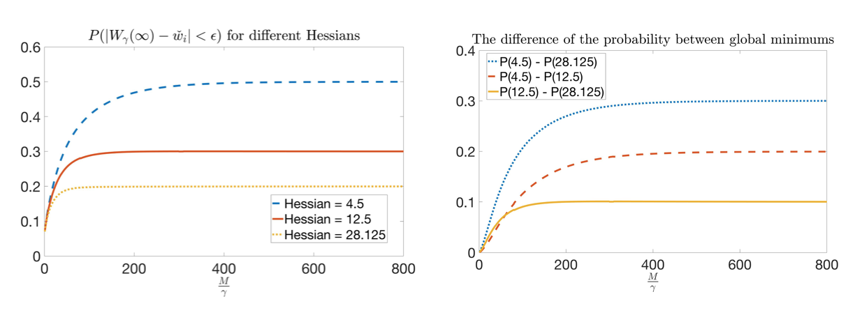
  • Example 1: Consider the risk function L(𝐰)𝐿𝐰L(\mathbf{w}) has three different global minima 𝐰isubscript𝐰𝑖\mathbf{w}_{i}, i=1,2,3𝑖123i=1,2,3, with different Hessians 4.54.54.5, 12.512.512.5, and 28.12528.12528.125, respectively. We are interested in the probability of the mini-batch SGD limk𝐰ksubscript𝑘subscript𝐰𝑘\lim_{k\to\infty}\mathbf{w}_{k} staying in the ϵitalic-ϵ\epsilon-neighborhood of global minima with respect to the ratio M/γ𝑀𝛾M/\gamma, where M𝑀M is the batch size and γ𝛾\gamma is the learning rate. The results are shown in Figure 6.

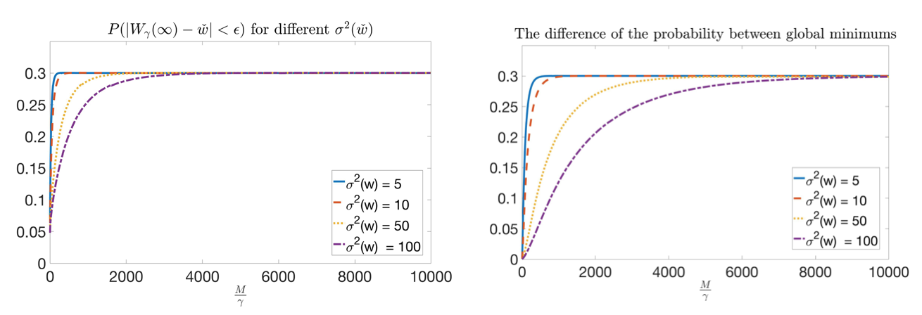
  • Example 2: Consider the variance of SGD has four different levels: 5,10,50,100510501005,10,50,100. We are interested in the probability of the mini-batch SGD limk𝐰ksubscript𝑘subscript𝐰𝑘\lim_{k\to\infty}\mathbf{w}_{k} staying in the ϵitalic-ϵ\epsilon-neighborhood of a same global minimum of L(𝐰)𝐿𝐰L(\mathbf{w}) with respect to the ratio M/γ𝑀𝛾M/\gamma. The results are shown in Figure 7.

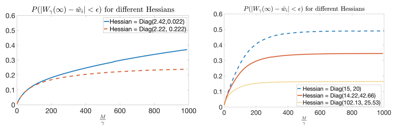
  • Example 3: Consider two-dimensional cases. We are interested in the risk function L(𝐰)𝐿𝐰L(\mathbf{w}) has two different global minima and furthermore, L(𝐰)𝐿𝐰L(\mathbf{w}) has two different global minima. For two minima case, we consider L(𝐰)𝐿𝐰L(\mathbf{w}) has two different Hessians (2.42,0.022)2.420.022(2.42,0.022) and (2.22,0.222)2.220.222(2.22,0.222). For three minima case, we consider L(𝐰)𝐿𝐰L(\mathbf{w}) has three different Hessians (15,20)1520(15,20), (14.22,42.66)14.2242.66(14.22,42.66), and (102.13,25.53)102.1325.53(102.13,25.53).

Refer to caption
Figure 6: Illustration of Example 1 with ϵ=0.1italic-ϵ0.1\epsilon=0.1. The left panel shows the probability of W()𝑊W(\infty) staying in the ϵitalic-ϵ\epsilon-neighborhood of different global minima. The right panel compares the differences of probabilities that W()𝑊W(\infty) staying in the ϵitalic-ϵ\epsilon-neighborhood of different global minima.
Refer to caption
Figure 7: Illustration of Example 1 with ϵ=0.1italic-ϵ0.1\epsilon=0.1. The left panel shows the probability of W()𝑊W(\infty) staying in the ϵitalic-ϵ\epsilon-neighborhood under different SGD variances σ2(𝐰ˇ)superscript𝜎2ˇ𝐰\sigma^{2}(\check{\mathbf{w}}). The right panel compares the differences of probabilities that W()𝑊W(\infty) staying in the ϵitalic-ϵ\epsilon-neighborhood of different σ(𝐰ˇ)𝜎ˇ𝐰\sigma(\check{\mathbf{w}}).
Refer to caption
Figure 8: Illustration of Example 3 with ϵ=0.1italic-ϵ0.1\epsilon=0.1. The left panel shows the probability of the limiting mini-batch SGD limk𝐰ksubscript𝑘subscript𝐰𝑘\lim_{k\to\infty}\mathbf{w}_{k} staying in the ϵitalic-ϵ\epsilon-neighborhood of two different global minima. The right panel shows the probability of three different global minima.

Results.

The results of Example 1 are given in Figure 6. We draw the following conclusions.

  • First, if the batch size M𝑀M and learning rate γ𝛾\gamma are the same, then 𝐖()𝐖\mathbf{W}(\infty) is more likely to stay near the flat minimum whose Hessian is smaller.

  • Second, as the ratio M/γ𝑀𝛾M/\gamma increases, the probability of 𝐖()𝐖\mathbf{W}(\infty) converging to a flatter minimum will increase faster than that of a sharper minimum.

  • Third, if the ratio of Hessians (the Hessian at a sharp minima divides the Hessian at a flat minima) increases, the difference of probabilities would increase as illustrated in the right panel of Figure 6. Moreover, if we increase the ratio M/γ𝑀𝛾M/\gamma, the difference of probabilities becomes more distinct.

The results of Example 2 are given in Figure 7. We draw the following conclusion.

  • If the variance σ(𝐰ˇ)𝜎ˇ𝐰\sigma(\check{\mathbf{w}}) increases, the effect of the ratio M/γ𝑀𝛾M/\gamma for the probability that converging to the global minimum will decrease. That implies as σ(𝐰ˇ)𝜎ˇ𝐰\sigma(\check{\mathbf{w}}) increases, the probability of SGD converging to a flat minimum will increase slower.

The results of Example 3 are given in Figure 8. We draw the following conclusion.

  • For a same ratio M/γ𝑀𝛾M/\gamma, if the product of the eigenvalues of the Hessian increases, then 𝐖()𝐖\mathbf{W}(\infty) will be more likely to stay near the minimum. For a same sharpness of the minimum, if one increase the batch size or decrease the learning rate, 𝐖()𝐖\mathbf{W}(\infty) will be more likely to stay near the minimum.

  • We conclude that the product of eigenvalues of the Hessian matrix will affect the probability of W()𝑊W(\infty) staying in the ϵitalic-ϵ\epsilon-neighborhood of the minimum, which is different from the sum of eigenvalues, the smallest eigenvalue, or the largest eigenvalue for multi-dimensional cases.

References

  • Anton. et al. [2001] Anton, A., Markowich, P., Toscani, G.  & Unterreiter, A.  (2001) On convex Sobolev inequalities and the rate of convergence to equilibrium for Fokker-Planck type equations. Communication in Partial Differential Equations 26(1–2):43-100.
  • Berglund [2013] Berglund, N.  (2013) Kramers’ law: Validity, derivations and generalisations. In Markov Processes Relat. Fields, 19:459-490.
  • Bovier et al. [2004] Bovier, A., Eckhoff, M., Gayrard, V.  & Klein, M.  (2004) Metastability in reversible diffusion processes I: Sharp asymptotics for capacities and exit times. In Journal of the European Mathematical Society, 6(4):399-424.
  • Bovier et al. [2005] Bovier, A. Gayrard, V.  & Klein, M.  (2004) Metastability in reversible diffusion processes II: Precise asymptotics for small eigenvalues. In Journal of the European Mathematical Society, 7(1):69-99.
  • Chaudhari et al. [2017] Chaudhari, P., Oberman, A., Osher, S., Soatto, S.  & Carlier, G.  (2017) Deep Relaxation: partial differential equations for optimizing deep neural networks. In International Conference on Learning Representations.
  • Chaudhari et al. [2017] Chaudhari, P.  & Soatto, S  (2017) Stochastic gradient descent performs variational inference, converges to limit cycles for deep networks arXiv preprint arXiv:1710.11029.
  • Choromanska et al. [2015] Choromanska, A., Henaff, M., Mathieu, M., Arous, G.B.  & LeCun, Y.  (2015) The loss surfaces of multilayer networks. In Res Math Sci, pp. 5–33.
  • Dauphin et al. [2014] Dauphin, Y.N., Pascanu, R., Gulcehre, C., Cho, K., Ganguli, S.  & Bengio, Y.  (2014) Identifying and attacking the saddle point problem in high-dimensional non-convex optimization. In Advances in Neural Information Processing Systems, pp.  2933–2941.
  • Dean et al. [2012] Dean, J., Corrado, G., Monga, R., Chen, K., Devin, M., Mao, M., Senior, A., Tucker, P., Yang, K., Le, Q.V.  & Ng, A.Y.  (2012) Large scale distributed deep networks. In Advances in Neural Information Processing Systems, pp. 1223–1231.
  • Dinh et al. [2017] Dinh, L., Pascanu, R., Bengio, S.  & Bengio, Y.  (2017) Sharp minima can generalize for deep nets. In International Conference on Machine Learning.
  • Dziugaite and Roy [2017] Dziugaite, G.K.  & Roy, D.M.  (2017) Computing nonvacuous generalization bounds for deep (stochastic) neural networks with many more parameters than training data. arXiv preprint arXiv:1703.11008.
  • Ge et al. [2015] Ge, R., Huang, R., Jin, C.  & Yuan, Y.  (2015) Escaping from saddle points–online stochastic gradient for tensor decomposition. In Conference on Learning Theory, pp. 797–842.
  • Hoffer et al. [2017] Hoffer, E., Hubara, I.  & Soudry, D.  (2017) Train longer, generalize better: closing the generalization gap in large batch training of neural networks. In Advances in Neural Information Processing Systems, pp.  1729–1739.
  • Jastrzebski et al. [2017] Jastrzebski, S., Kenton, Z., Arpit, D., Ballas, N., Fischer, A., Bengio, Y.  & Storkey, A.  (2017) Three factors influencing minima in SGD. In arXiv preprint arXiv:1711.04623.
  • Keskar et al. [2017] Keskar, N.S., Mudigere, D., Nocedal, J., Smelyanskiy, M.  & Tang, P.T.P.  (2017) On large-batch training for deep learning: Generalization gap and sharp minima. In International Conference on Learning Representations.
  • Kolpas. et al. [2007] Kolpas, A., Moehlis, J.  & Kevrekidis, I.G.  (2007) Coarse-grained analysis of stochasticity-induced switching between collective motion states. Proceedings of the National Academy of Sciences 104(14):5931-5935.
  • LeCun et al. [1998] LeCun, Y., Bottou, L., Orr, G.B.  & Müller, K.R.  (1998) Efficient backprop. In Neural networks: Tricks of the trade, pp. 9–50. Springer, Berlin, Heidelberg.
  • Li et al. [2017] Li, Q., Tai, C.  & E, W.  (2017) Stochastic modified equations and adaptive stochastic gradient algorithms. arXiv preprint arXiv:1511.06251.
  • Mandt et al. [2017] Mandt, S., Hoffman, M.D.  & Blei, D.M.  (2017) Stochastic gradient descent as approximate bayesian inference In Journal of Machine Learning Research 18:1-35.
  • Pavliotis [2014] Pavliotis, G.A.  (2014) Stochastic processes and applications: diffusion processes, the Fokker-Planck and Langevin equations. Springer.
  • Pavliotis [2018] Pavliotis, G.A.  (2014) Stochastic processes and applications: Diffusion processes, the Fokker-Planck and Langevin equations. Springer.
  • Poggio [2017] Poggio, T., Kawaguchi, K., Liao, Q., Miranda, B., Rosasco, L., Boix, X., Hidary, J.  & Mhaskar, H.  (2017) Theory of Deep Learning III: explaining the non-overfitting puzzle. arXiv preprint arXiv:1801.00173.
  • Pólya [1945] Pólya, G.  (1945) Remarks on computing the probability integral in one and two dimensions. In Proceedings of the 1st Berkeley Symposium on Mathematical Statistics and Probability
  • Raginsky [2017] Raginsky, M., Rakhlin, A.  & Telgarsky, M.  (2017) Non-convex learning via Stochastic Gradient Langevin Dynamics: a nonasymptotic analysis. arXiv preprint arXiv:1702.03849.
  • Wu and Zhu [2017] Wu, L..  & Zhu, Z.  (2017) Towards Understanding Generalization of Deep Learning: Perspective of Loss Landscapes. arXiv preprint arXiv:1706.10239.
  • Zhang et al. [2017] Zhang, C., Bengio, S., Hardt, M., Recht, B.  & Vinyals, O.  (2017) Understanding deep learning requires rethinking generalization. In International Conference on Learning Representations.