Finite-energy dressed string-inspired Dirac-like monopoles

Abstract

Abstract

On extending the Standard Model (SM) Lagrangian, through a non-linear Born-Infeld (BI) hypercharge term with a parameter $\beta$ (of dimensions of [mass]²), a finite energy monopole solution was claimed by Arunasalam and Kobakhidze AK . We report on a new class of solutions within this framework which was missed in the earlier analysis. This new class was discovered on performing consistent analytic asymptotic analyses of the nonlinear differential equations describing the model; the shooting method used in numerical solutions to boundary value problems for ordinary differential equations is replaced in our approach by a method which uses diagonal Padé approximants. Our work uses the ansatz proposed by Cho and Maison CM to generate a static and spherically symmetric monopole with finite energy and differs from that used in the solution of AK . Estimates of the total energy of the monopole are given, and detection prospects at colliders are briefly discussed.

I Introduction

It is a curious fact that Maxwell initially wrote as one of his eponymous equations:

$$curl\,\vec{A}=\mu\vec{H}.$$ (1)

The magnetic field is denoted by $\vec{H}$; $\vec{A}$ is the electromagnetic vector potential and $\mu$ is the magnetic permeability. If $\vec{A}$ is a non-singular vector then

$$\vec{\nabla}\cdot\vec{H}=0.$$ (2)

In 1931 Dirac dirac considered a singular $\vec{A}$ field. If $\vec{n}$ is a constant unit vector in the $z$-direction, then the vector potential has the form

$$\vec{A}\left({\vec{r}}\right)=g^{m}\,\frac{{\vec{r}\times\vec{n}}}{{r\left({r-\vec{r}\cdot\vec{n}}\right)}},$$ (3)

with $g^{m}$ the magnetic charge dirac , which has a singularity along the positive $z$-axis known as a Dirac string. On calculating $curl\,\vec{A}$ we find a magnetic field of a monopole

$$\vec{B}\left({\vec{r}}\right)=g^{m}\,\tfrac{{\vec{r}}}{{{r^{3}}}}$$ (4)

except along the string. In classical physics the string should play no role in the dynamics of particles because of its infinitesimal nature. In quantum theory the situation is different since the wave function $\Psi$ of a non-relativistic particle with charge $e$ and mass $m$ in a monopole background satisfies

$$i\frac{\partial}{{\partial t}}\Psi=-\frac{{{{\left({\vec{\nabla}-ie\vec{A}}\right)}^{2}}}}{{2m}}\Psi$$ (5)

which has the stationary solution

$$\Psi\left({\vec{r}}\right)={\Psi_{0}}\left({\vec{r}}\right)\exp\left[{ie\int\limits_{0}^{\vec{r}}{d\vec{x}.\vec{A}\left({\vec{x}}\right)}}\right].$$ (6)

The wave function $\Psi\left({\vec{r}}\right)$ is single valued and so there should be no change in $\Psi\left({\vec{r}}\right)$ for a small circuit $C$ around the string. The change in the argument of the exponential in (6) along $C$ should be of the form $2n\pi i$ where $n$ is an integer. This leads to the condition

$$e\oint_{C}{d\vec{x}\cdot\vec{A}\left({\vec{x}}\right)=2\pi n}.$$ (7)

Since the magnetic flux through the circuit $C$ is $4\pi g^{m}$, from (7) we deduce deduce the celebrated Dirac charge quantisation condition dirac

$$eg^{m}=\frac{n}{2},\quad n\in{\mathbf{Z}}\,{\rm U}\,\{0\},$$ (8)

or, equivalently

$$g^{m}=\frac{1}{2\,\alpha}\,n\,e=g_{D}n,\quad g_{D}\equiv\frac{1}{2\,\alpha},\quad n\in{\mathbf{Z}}\,{\rm U}\,\{0\},$$ (9)

where $\alpha$ is the fine structure constant, which at low (strictly speaking zero) energy has the value $\alpha=1/137$, and $g_{D}=68.5$ is the fundamental Dirac charge.

The Standard Model of particle physics has been developed subsequent to the original work of Dirac. It describes the weak, electromagnetic and strong interactions of leptons and hadrons. It is important to ascertain how monopoles may fit into the electro-weak sector of the SM, in part because of the possible detectability of electro-weak monopoles (of mass a few TeV) at colliders in the near future. The work of ‘t Hooft and Polyakov hpmono provides a detailed paradigm on magnetic monopole soliton solutions, which arise in quantum field theories with simple gauge groups (such as SU(3) and Grand Unified groups SU(5)), under spontaneous symmetry breaking. In such solutions, Dirac’s quantisation arises as a topological property of mappings associated with the solution and not because of a Dirac string.

The SM does not have a simple group, as the gauge group of the electroweak sector is $SU(2)\times U_{Y}(1)$, with $U_{Y}(1)$ the weak hypercharge gauge group. This was one of the arguments against any attempts to find a topological monopole solution within the SM. Nevertheless, Cho and Maison (CM) CM presented a monopole solution within the $SU(2)\times U_{Y}(1)$ electroweak theory, by arguing that a non-trivial topology of th solutions was still possible due to an underlying $CP^{1}$ structure. Specifically, Cho and Maison view the normalised Higgs doublet field of the SM in the symmetry broken phase as a $CP^{1}$ field, which is known to have a non-trivial second homotopy $\Pi_{2}(CP^{1})={\tt\mathbb{Z}}$; it was argued CM that this homotopy would lead to a charge quantisation of the monopole as in the ’Hooft-Polyakov case. In CM the monopole and dyon solutions (characterised by both electric and magnetic charges), suffer, however, from ultraviolet infinities in their total energy. This casts serious doubts on the existence of consistent soliton solutions (which by definition have finite energy).

The considerations above suggest that the model needs a modification before any physical conclusions can be drawn drawn. Examples of a modification of the theory beyond the SM, are inclusion of non-minimal couplings of the Higgs field with the hypercharge kinetic terms in the effective Lagrangian CKY ; you , or through higher derivative extensions, such as a non-linear Born-Infeld gauge field theory, which notably arises as a low energy field theory limit of strings gsw . Although in string theory, the full standard model gauge group admits such non-linear extensions, nonetheless, it suffices for our phenomenological purposes to restrict our attention only to the Born-Infeld extension of the hypercharge sector, and seek monopole solutions of CM type, following  AK   .

The finiteness of the monopole solution in Born-Infeld type theories is an immediate consequence of the finiteness of the electromagnetic field energy density in Born-Infeld non-linear electrodynamics zwiebach .The identification of finite energy consistent monopole solutions in (extensions of) the SM, represents not only an important theoretical advance, but also an important step towards a consistent phenomenology since one can provide estimates of the total energy/mass of monopoles and thus check the feasibility of their production at colliders vento . Recently experimental efforts to discover monopoles have redoubled atlas ; moedal . In particular, searches for magnetic monopoles of lowest magnetic charge are ongoing in the ATLAS-LHC experiment atlas . In addition, the MoEDAL experiment at the LHC moedal is geared to the detection of highly ionising particles, among which magnetic monopoles, using a variety of experimental techniques, which allow for monopoles of high magnetic charge to be searched for for the first time in experiment. From the arguments of Dirac the monopole magnetic charge would be an integer multiple of ${g_{D}}\left({=68.5}\right)$ (9). Consequently magnetic monopoles interact strongly with photons and are highly ionising, making TeV mass monopoles candidates suitable for detection at MoEDAL moedal . However, as argued in  drukier , structured monopoles, such as the ones mentioned above (which arise as consistent solutions of specific quantum gauge field theories with spontaneous symmetry breaking), might exhibit extremely suppressed production cross-sections. This suppression would eliminate any prospect for detection for structured monopoles. Dirac (structureless) monopoles do not suffer from suppressed production cross-sections. Nonetheless, finite-energy structured monopoles, might be produced abundantly from the vacuum via a thermal version of the Schwinger pair production, as advocated in rajantie , and, hence, can still be of great relevance to heavy ion collisions at LHC. If they have sufficiently low mass the monopoles can be potentially detected by the deployment of magnetic monopole trapping detectors (of the type used in MoEDAL moedal ) in such environments rajantie2 .

We now remark that the monopole solutions discussed in AK , and also in the previous literature of the electroweak monopole CM ; CKY (and its finite energy extensions you ) are based on matching numerical solutions using shooting methods. Such solutions, however, appear not to be in agreement with next to leading order analytical solutions near the monopole centre. It is the purpose of this work, to discuss a new class of solutions, which match an analytic asymptotic behaviour at both small and large distances from the monopole centre. The solutions are slightly different near the monopole centre from the standard electroweak monopole solutions appeared in the literature CM ; CKY ; AK ; you . Nevertheless, as we demonstrate in the present article, the order of magnitude of the associated total energy (of crucial importance for their phenomenology) remains the same as in the standard CM-like case AK . Current experimental lower bounds of the Born-Infeld mass parameter then, imply monopole masses of at least 11 TeV, which makes such solutions relevant for potential detection only at future colliders you2 .

The structure of the article is as follows: in the next section II we introduce the model and give the dynamical equations that will be associated with monopole solutions (but not dyon solutions). In the following section, III we discuss our new solutions, which have not appeared before in the literature. We discuss analytic forms of the solutions for short and large distances from the monopole centre, and the associated interpolating functions, found by using Padé approximant methods AAMC ; GB . Energy estimates and thus detection prospects, are discussed in section IV. Finally, our conclusions and outlook are presented in section V.

II Born-Infeld Electroweak Monopole: the set up

A string-inspired extension (ESM) of the SM, considered in AK and used in the current work, arises when the standard kinetic energy of the hypercharge gauge field is replaced by a non-linear Born-Infeld term zwiebach . The resultant Lagrangian is

$$\mathcal{L}_{EW}=-(D_{\mu}H)^{\dagger}(D^{\mu}H)-\frac{\lambda}{2}\Big{(}H^{\dagger}H-\frac{\mu^{2}}{\lambda}\Big{)}^{2}-\frac{1}{4}F^{a}_{\mu\nu}F^{\mu\nu,a}+\beta^{2}\Big{(}1-\sqrt{1+\frac{1}{2\beta^{2}}B_{\mu\nu}B^{\mu\nu}-\frac{1}{16\beta^{4}}(B_{\mu\nu}\tilde{B}^{\mu\nu})^{2}}\Big{)}$$ (10)

where: $A^{a}_{\mu}$ and $B_{\mu}$ are the $SU(2)$ and $U_{Y}(1)$ gauge fields respectively; $B^{\mu\nu}$ is the $U_{Y}(1)$ field strength tensor; $\tilde{B}_{\mu\nu}=\frac{1}{2}\,\epsilon_{\mu\nu\rho\sigma}\,B^{\rho\sigma}$ (with $\epsilon_{\mu\nu\rho\sigma}$ being the covariant Levi-Civita fully antisymmetric tensor); $F^{\mu\nu,a}$ ($a=1,2,3$) is the $SU(2)$ field strength tensor; $D_{\mu}=\partial_{\mu}-i\frac{g}{2}\tau^{a}A^{a}_{\mu}-i\frac{g^{\prime}}{2}B_{\mu}$ is the covariant derivative with, $\tau_{a}$, $a=1,2,3,$ the Pauli $2\times 2$ matrices; $\frac{\tau_{a}}{2}$, $a=1,2,3$ are the SU(2) generators; $H$ is the electroweak Higgs doublet. The $SU(2)$ and $U_{Y}(1)$ couplings are given by $g$ and $g^{\prime}$ respectively, with

$$g^{\prime}=g\,{\rm tan}\theta_{W},$$ (11)

where $\theta_{W}$ is the SM weak mixing angle. The Born-Infeld parameter $\beta$ has dimensions of [mass]². The ESM Lagrangian reduces formally to the SM Lagrangian for $\beta\rightarrow\infty$. In the context of microscopic string theory models, the parameter $\sqrt{\beta}\propto M_{s}$, the string mass scale. In our phenomenological approach here, we deviate from this restriction, and treat $\beta$ as a free parameter to be constrained by experiment, as we shall discuss in secrtion IV.

We shall be interested in finite energy classical monopole solutions of Cho-Maison (CM) type CM , for the Euler-Lagrange equations of ESM for finite $\beta$. In the limit $\beta\to\infty$ one would recover the formal CM monopole solution with divergent energy. The equations of motion, stemming from (10) read:

$$D^{\mu}(D_{\mu}H)=\lambda\Big{(}H^{\dagger}H-\frac{\mu^{2}}{\lambda}\Big{)}H,$$ (12)

$$\partial_{\mu}F^{\mu\nu,a}+gf^{abc}A_{\mu}^{b}F^{\mu\nu,c}=\frac{ig}{2}\Big{[}H^{\dagger}\tau^{a}(D^{\nu}H)-(D^{\nu}H)^{\dagger}\tau^{a}H\Big{]},$$ (13)

$$\partial_{\mu}\Big{[}\frac{B^{\mu\nu}-\frac{1}{4\beta^{2}}(B_{\alpha\beta}\tilde{B}^{\alpha\beta})\tilde{B}^{\mu\nu}}{\sqrt{1+\frac{1}{2\beta^{2}}B_{\alpha\beta}B^{\alpha\beta}-\frac{1}{16\beta^{4}}(B_{\alpha\beta}\tilde{B}^{\alpha\beta})^{2}}}\Big{]}=i\frac{g^{\prime}}{2}\big{[}H^{\dagger}(D^{\nu}H)-(D^{\nu}H)^{\dagger}H\big{]}.$$ (14)

The following ansatz is used to determine the energy of the charged solutions to this Lagrangian CM :

$$H=\frac{1}{\sqrt{2}}\rho(r)\xi$$

$$A^{a}_{\mu}=\frac{1}{g}{\cal{A}}(r)\partial_{\mu}t\,\hat{\phi}^{a}+\frac{1}{g}(f(r)-1)\,\epsilon_{abc}\,\hat{\phi}^{b}(\partial_{\mu}\,\hat{\phi}^{c})$$ (15)

$$B_{\mu}=-\frac{1}{g^{\prime}}{\cal{B}}(r)\partial_{\mu}t-\frac{1}{g^{\prime}}(1-cos(\theta))\partial_{\mu}\psi$$

where

$$\xi=i\begin{bmatrix}sin(\theta/2)e^{-i\psi}\\ -cos(\theta/2)\end{bmatrix}.$$

Here, $r^{a}=(t,r,\theta,\psi)$ are spherical polar coordinates (with $0\leq\theta\leq\pi$ , $0\leq\phi<2\pi$ ) and

$$\hat{\phi}^{a}=\xi^{\dagger}\tau^{a}\xi=-\hat{r}^{a},$$

where the circumflex denotes unit vector.

The ansatz (II) is best physically understood if one performs a gauge rotation to the unitary
gauge CM ; CKY :

$$\xi\quad\rightarrow U\,\xi=\begin{pmatrix}1\\ 0\end{pmatrix},\quad{\rm with}\quad U=\begin{pmatrix}\cos(\theta/2)&\sin(\theta/2)\,e^{-i\psi}\\ -\sin(\theta/2)\,e^{i\psi}&\cos(\theta/2)\end{pmatrix}~{},$$ (16)

under which the non-Abelian field transforms to

$$\vec{A}_{\mu}=\frac{1}{g}\,\begin{pmatrix}-f(r)\,\sin(\psi)\,\partial_{\mu}\theta+\sin(\theta)\,\cos(\psi)\,\partial_{\mu}\psi\\ f(r)\,\cos(\psi)\,\partial_{\mu}\theta-\sin(\theta)\,\sin(\psi)\,\partial_{\mu}\psi\\ {\cal{A}}(r)\,\partial_{\mu}t-\big{(}1-\cos(\theta)\big{)}\,\partial_{\mu}\psi\end{pmatrix}.$$ (17)

The physical fields, the electromagnetic potential $A_{\mu}^{\rm em}$ and the neutral $Z^{0}_{\mu}$ gauge boson field involve the weak mixing angle $\theta_{W}$, and are given by CM :

$$\begin{pmatrix}A_{\mu}^{\rm em}\\ Z^{0}_{\mu}\end{pmatrix}=\begin{pmatrix}\cos(\theta_{W})&\sin(\theta_{W})\\ -\sin(\theta_{W})&\cos(\theta_{W})\end{pmatrix}\,\begin{pmatrix}B_{\mu}\\ A_{\mu}^{3}\end{pmatrix}=\frac{1}{\sqrt{g^{2}+(g^{\prime})^{2}}}\,\begin{pmatrix}g&g^{\prime}\\ -g^{\prime}&g\end{pmatrix}\,\begin{pmatrix}B_{\mu}\\ A_{\mu}^{3}\end{pmatrix},$$ (18)

on taking into account (11). In summary the ansatz (II) yields the physical fields of the SM CM :

$${\rm W_{\mu}^{\pm}} \equiv \frac{1}{\sqrt{2}}\Big{(}A_{\mu}^{1}\mp iA_{\mu}^{2}\Big{)}=\frac{1\,}{g\,\sqrt{2}}\,\Big{(}\mp if\left(r\right)\partial_{\mu}\theta\exp\left(\mp i\psi\right)+\sin(\theta)\,\partial\psi\exp\left(\pm i\psi\right)\Big{)}$$

$$A_{\mu}^{\rm em} = e\,\Big{(}\frac{1}{g^{2}}\,{\cal{A}}(r)+\frac{1}{(g^{\prime})^{2}}\,{\cal{B}}(r)\Big{)}\,\partial_{\mu}t-\frac{1}{e}\Big{(}1-\cos(\theta)\Big{)}\,\partial_{\mu}\psi,$$ (19)

$$Z^{0}_{\mu} = \frac{e}{g^{\prime}\,g}\Big{(}{\cal{A}}(r)-{\cal{B}}(r)\Big{)}\,\partial_{\mu}t,$$

with

$$e=g\,\sin(\theta_{W})=\frac{g\,g^{\prime}}{\sqrt{g^{2}+(g^{\prime})^{2}}},$$ (20)

the electron charge. As can be seen from (II), the spherically symmetric (static) monopole solution of CM is characterised by:

$${\cal{A}}(r)={\cal{B}}(r)=0.$$ (21)

In this case the electromagnetic potential resembles a Dirac point-like monopole,

$$A_{\mu}^{\rm em}=-\frac{1}{e}\Big{(}1-\cos(\theta)\Big{)}\,\partial_{\mu}\psi,$$ (22)

but the magnetic charge $g^{m}$ is twice the fundamental Dirac charge; so

$$g^{m}=\frac{4\pi}{e}=\frac{4\pi\,\sqrt{g^{2}+(g^{\prime})^{2}}}{g\,g^{\prime}}~{},$$ (23)

where in the last equality we used (20).

If (21) is valid, from (II) the $Z_{\mu}^{0}$ configuration vanishes,

$$Z_{\mu}^{0}=0.$$ (24)

and moreover the expressions (II) reduce to

$$H=\frac{1}{\sqrt{2}}\rho(r)\xi$$

$$A^{a}_{\mu}=\frac{1}{g}(f(r)-1)\epsilon_{abc}\,\hat{\phi}^{b}(\partial_{\mu}\hat{\phi}^{c})$$ (25)

$$B_{\mu}=-\frac{1}{g^{\prime}}(1-cos(\theta))\partial_{\mu}\psi.$$

and the equation for the hypercharge gauge boson (14) is trivially satisfied. From (II), we also note that the hypercharge-sector ‘magnetic field’ $\mathcal{B}^{Y}_{i}=\epsilon_{ijk}\,\partial^{j}B^{k}$ corresponding to $B_{\mu}$, assumes the following for the monopole solution:

$$\vec{{\mathcal{B}}^{Y}}=\Big{(}\frac{4\pi}{g^{\prime}}\Big{)}^{2}\frac{\vec{r}}{r^{3}}.$$ (31)

This has the same singular form (as $r\to 0$) as the monopole magnetic field (27), but with the magnetic charge being replaced by the ‘hypermagnetic charge $g_{Y}^{m}\equiv\frac{4\pi}{g^{\prime}}$. We shall make use of (31), when we evaluate the total energy of the Born-Infeld-Cho-Maison-like solution in section IV.

From now we will concentrate on the equations of motion for the Higgs field and $SU(2)$
gauge field, (12) and (13), respectively; these equations coincide with those in the
ordinary CM case CM . On using (II), these become

$${\rho}^{\prime\prime}+\frac{2}{r}{\rho}^{\prime}-\frac{f^{2}}{2r^{2}}\rho=\lambda\Big{(}\frac{\rho^{2}}{2}-\frac{\mu^{2}}{\lambda}\Big{)}\rho$$ (32a)

$${f}^{\prime\prime}-\frac{f^{2}-1}{r^{2}}f=\frac{g^{2}}{4}\,\rho^{2}\,f,$$ (32b)

$${\cal{A}}^{\prime\prime}+\frac{2}{r}\,{\cal{A}}^{\prime}-2\frac{f^{2}}{r^{2}}\,{\cal{A}}=\frac{g^{2}}{4}\,\rho^{2}\,\Big{(}{\cal{A}}-{\cal{B}}\Big{)}$$ (32c)

where the prime denotes differentiation with respect to $r$. For the monopole solution, for which (21) is valid, the third of the above equations is trivially satisfied, yielding zero on both sides. The trivial solution of the equations of motion (32), which yields the Dirac monopole, has no
W${}^{\pm}_{\mu}$-bosons, that is

$$f(r)=0~{},\quad{\rm and}\quad\rho=\rho_{0}=\sqrt{\frac{2\mu^{2}}{\lambda}}\neq 0,$$ (33)

with $\rho_{0}$ the Higgs field vacuum expectation value (vev) in the broken symmetry phase.

III New solutions for Born-Infeld-inspired electroweak dressed magnetic monopoles

We shall consider new solutions of (32) where we still have (21) but $f(r)$ and $\rho(r)$ are
allowed to be non-trivial. Such solutions can be interpreted as Dirac monopoles dressed by W${}^{\pm}_{\mu}$-bosons and have not been discussed so far in the literature. We seek solutions of (32) for $\rho(r)$ and $f(r)$ which satisfy the following boundary conditions

$$f(r=0) =1,\;\;\rho(r=0)=0,$$

$$f(r=\infty) =0,\;\;\rho(r=\infty)=\rho_{0}=\sqrt{\frac{2\mu^{2}}{\lambda}}\neq 0.$$ (34)

Before further analysis we will rewrite the equations (32) in terms of dimensionless quantities:

$$\tilde{\rho}=\frac{\rho}{{{\rho_{0}}}},$$

$$\varepsilon=\frac{{{g^{2}}}}{{2\lambda}},$$

and

$$x=\mu r.$$

Hence the dimensionless forms of the first two equations of (32) are:

$$\tilde{\rho}^{\prime\prime}\left(x\right)+\frac{2}{x}\tilde{\rho}^{\prime}\left(x\right)-\frac{{{f^{2}}\left(x\right)}}{{2{x^{2}}}}\tilde{\rho}\left(x\right)=\tilde{\rho}\left(x\right)\left({{{\tilde{\rho}}^{2}}\left(x\right)-1}\right)$$ (35)

and

$$f^{\prime\prime}\left(x\right)-\frac{{{f^{2}}\left(x\right)-1}}{{{x^{2}}}}f\left(x\right)=\varepsilon{{\tilde{\rho}}^{2}}\left(x\right)f\left(x\right)$$ (36)

where ^′ denotes $\frac{d}{{dx}}$. The boundary conditions for $\tilde{\rho}\left(x\right)$ are $\tilde{\rho}(x=0)=0$ and $\tilde{\rho}(x=\infty)=1$. It is important to note that, from (35), $f^{2}\left(x\right)$ is determined in terms of $\tilde{\rho}$ and its derivatives.

The system of equations (35) and (36) are usually solved numerically CM ; AK ; however there is a delicate interplay in the small $x$ behaviour of $f\left(x\right)$ and $\tilde{\rho}\left(x\right)$ which purely numerical solutions can miss. The equations (III), (35) and (36) represent a boundary value. Unlike initial value problems, boundary value problems are not guaranteed to have a unique solution; in some instances there may be no solution at all. Coupled boundary value problems pose an additional challenge since approximations for $\tilde{\rho}$ and $f$ cannot be made independently. We will first obtain asymptotic expansions as $x\to 0$ and as $x\to\infty$. From these asymptotic expansions and a smooth interpolating function we can evaluate the energy of the monopole within ESM.

The matching of the asymptotic expansions for large and small $x$ would result in an interpolating solution; this matching is, however, not straightforward. Consequently we will take a different approach to determining a suitable interpolating function based on a Padé approximant for a small $x$ asymptotic series. We take $\varepsilon\sim.81$ which is obtained from values of the parameters phenomenologically relevant for SM, namely, $g\simeq 0.65$ and $\lambda\simeq.26$.

III.1 Large $x$ asymptotics

Respecting the boundary conditions (III) we write $\tilde{\rho}\left(x\right)=1+\tilde{\delta}\left(x\right)$ with $\left|{\tilde{\delta}\left(x\right)}\right|\ll 1$. To leading order then (36) becomes

$$f^{\prime\prime}\left(x\right)+\frac{{f\left(x\right)}}{{{x^{2}}}}=\varepsilon f\left(x\right).$$ (37)

Similarly (35) becomes

$$\tilde{\delta}^{\prime\prime}\left(x\right)+\frac{2}{x}\tilde{\delta}^{\prime}\left(x\right)-2\tilde{\delta}\left(x\right)=\frac{{{f^{2}}\left(x\right)}}{{2{x^{2}}}}.$$ (38)

III.1.1 Behaviour of $f\left(x\right)$

The leading behaviour of (37) is governed by

$$f^{\prime\prime}\left(x\right)=\varepsilon f\left(x\right)$$ (39)

and the solution compatible with the boundary conditions is $f\left(x\right)={f_{1}}\exp\left({-\sqrt{\varepsilon}x}\right).$ In order to include the subleading behaviour we write $f\left(x\right)={f_{1}}\exp\left({-\sqrt{\varepsilon}x}\right)+\Delta\left(x\right)$ where

$$\Delta^{\prime\prime}\left(x\right)-\varepsilon{\kern 1.0pt}\Delta\left(x\right)=-\frac{{{f_{1}}}}{{{x^{2}}}}\exp\left({-\sqrt{\varepsilon}x}\right).$$ (40)

A particular solution ${\Delta_{p}}\left(x\right)$ of this inhomogeneous second order differential equation (using the method of variation of parameters) is

$${\Delta_{p}}\left(x\right)=\frac{{\exp\left({-\sqrt{\varepsilon}x}\right)}}{{2\sqrt{\varepsilon}}}\int\limits^{x}{dt\frac{{{f_{1}}}}{{{t^{2}}}}\;-\;}\frac{{\exp\left({\sqrt{\varepsilon}x}\right)}}{{2\sqrt{\varepsilon}}}\int\limits^{x}{dt\frac{{{f_{1}}}}{{{t^{2}}}}}\exp\left({-2\sqrt{\varepsilon}t}\right)$$ (41)

and the resultant $f(x)=f_{\infty}(x)$ is

$$f_{\infty}\left(x\right)\sim\exp\left({-\sqrt{\varepsilon}x}\right)\left[{{d_{1}}-\frac{{{f_{1}}}}{{2\sqrt{\varepsilon}x}}\left({1-\frac{1}{{2\sqrt{\varepsilon}x}}+O\left({\frac{1}{{{x^{2}}}}}\right)}\right)}\right].$$ (42)

III.1.2 Behaviour of $\tilde{\delta}\left(x\right)$

We shall now consider the inhomogeneous equation (38). In terms of

$$F\left(x\right)\equiv\frac{{f_{\infty}^{2}\left(x\right)}}{{2{x^{2}}}}$$

a particular solution ${{\tilde{\delta}}_{p}}\left(x\right)$ of (38) is given by

$${{\tilde{\delta}}_{p}}\left(x\right)=\frac{1}{{2\sqrt{2}}}\left({-\exp\left({-\sqrt{2}x}\right)\int\limits^{x}{t\exp\left({\sqrt{2}t}\right)F\left(t\right)dt+\exp\left({\sqrt{2}x}\right)\int\limits^{x}{t\exp\left({-\sqrt{2}t}\right)F\left(t\right)dt}}}\right).$$ (43)

The asymptotic expansion of $\tilde{\rho}(x)$ is then given by $1+{{\tilde{\delta}}_{p}}\left(x\right)+{d_{2}}\frac{{\exp\left({-\sqrt{2}x}\right)}}{x}$ where we have added
a solution of the homogeneous equation and

$$\widetilde{\delta}_{p}\left(x\right)=-\frac{d_{1}}{2\sqrt{2}x}\left[\frac{f_{1}}{2\sqrt{\varepsilon}}\exp\left(-2\sqrt{\varepsilon}x\right)+\frac{\sqrt{2}f_{1}\left(\sqrt{2\varepsilon}-1\right)+\sqrt{\varepsilon}d_{1}}{2\sqrt{2\varepsilon}\left(\sqrt{2\varepsilon}-1\right)}\exp\left(-2\left(\sqrt{2}-\sqrt{\varepsilon}\right)x\right)\right].$$ (44)

The dominant exponential in (44) as $x\to\infty$ is $\exp\left(-2\left(\sqrt{2}-\sqrt{\varepsilon}\right)x\right)$.

III.2 Small $x$ asymptotics

We write $f\left(x\right)=1+{\Delta_{0}}\left(x\right)$ with ${\Delta_{0}}\left(x\right)\to 0$ as $x\to 0$ and the leading behaviour in this limit is determined by

$${\Delta_{0}}^{\prime\prime}\left(x\right)-\frac{2}{{{x^{2}}}}{\Delta_{0}}\left(x\right)=\varepsilon{\kern 1.0pt}{{\tilde{\rho}}^{2}}\left(x\right).$$ (45)

For our solution it is important to note that ${{\tilde{\rho}}^{2}}\left(x\right)$ is not assumed to be small in comparison with ${\Delta_{0}}\left(x\right)$. The remaining equation to be considered is

$$\tilde{\rho}^{\prime\prime}\left(x\right)+\frac{2}{x}\tilde{\rho}^{\prime}\left(x\right)+\left({1-\frac{1}{{2{x^{2}}}}}\right)\tilde{\rho}\left(x\right)=0$$ (46)

which has a solution $\tilde{\rho}\left(x\right)\propto{j_{\delta}}\left(x\right)\left({\equiv\sqrt{\frac{\pi}{{2x}}}{J_{\delta+\frac{1}{2}}}\left(x\right)}\right)$ where $\delta=\frac{{\sqrt{3}-1}}{2}$. From the power series for Bessel functions we have

$${j_{\delta}}\left(x\right)=\frac{{\sqrt{\pi}}}{2}{x^{\delta}}\sum\limits_{m=0}^{\infty}{\frac{{{{\left({-1}\right)}^{m}}}}{{m!}}}\frac{{{{\left({x/2}\right)}^{2m}}}}{{\Gamma\left({\delta+m+3/2}\right)}}.$$

To low order in $x$

$$\tilde{\rho}\left(x\right)\simeq{c_{1}}{x^{\delta}}\left({1-\frac{{{x^{2}}}}{{2\left({2\delta+3}\right)}}}\right).$$ (47)

From (45) and (47) we deduce that

$${\Delta_{0}}^{\prime\prime}\left(x\right)-\frac{2}{{{x^{2}}}}{\Delta_{0}}\left(x\right)=\varepsilon{\kern 1.0pt}c_{1}^{2}{x^{2\delta}}{\left({1-\frac{{{x^{2}}}}{{2\left({2\delta+3}\right)}}}\right)^{2}}.$$ (48)

The relevant particular solution ${\Delta_{0p}}\left(x\right)$ of (48) is

$${\Delta_{0p}}\left(x\right)=\frac{{\varepsilon{\kern 1.0pt}c_{1}^{2}}}{3}{x^{2+2\delta}}\left[{\frac{3}{{2\delta\left({3+2\delta}\right)}}-\frac{{3{x^{2}}}}{2}{{\left({15+31\delta+20{\delta^{2}}+4{\delta^{3}}}\right)}^{-1}}+O\left({{x^{4}}}\right)}\right].$$ (49)

III.3 Summary of leading asymptotic solutions

We shall for convenience gather together the results of our asymptotic analysis.

For small $x$ :

$$\tilde{\rho}\left(x\right)\sim{c_{1}}{x^{\delta}}\left({1-\frac{{{x^{2}}}}{{2\left({2\delta+3}\right)}}}\right),$$

$$f\left(x\right)\sim 1+\frac{{\varepsilon{\kern 1.0pt}c_{1}^{2}}}{2}{x^{2+2\delta}}\left({\frac{1}{{\delta\left({3+2\delta}\right)}}-\frac{{{x^{2}}}}{{15+31\delta+20{\delta^{2}}+4{\delta^{3}}}}+O\left({{x^{4}}}\right)}\right).$$ (50)

It is interesting to note that our asymptotic analysis has revealed a ”bump” in $f\left(x\right)$ for small $x$.

For large $x$:

$$f\left(x\right)\sim\exp\left({-\sqrt{\varepsilon}x}\right)\left({{d_{1}}-\frac{{{f_{1}}}}{{2\sqrt{\varepsilon}x}}\left({1-\frac{1}{{2\sqrt{\varepsilon}x}}+\frac{1}{{2\varepsilon{x^{2}}}}}\right)}\right),$$ (51)

$$\rho\left(x\right)\sim 1+{d_{2}}\frac{{\exp\left({-\sqrt{2}x}\right)}}{x}-\frac{1}{{2\sqrt{2}}}\left(\begin{array}[]{l}\frac{{{d_{1}}{f_{1}}}}{{2\sqrt{\varepsilon}x}}\exp\left({-2\sqrt{\varepsilon}x}\right)\\ +\frac{{\exp\left({-2\left({\sqrt{2}-\sqrt{\varepsilon}}\right)x}\right)}}{x}\frac{{{d_{1}}\left({\sqrt{2}{f_{1}}\left({\sqrt{2\varepsilon}-1}\right)+\sqrt{\varepsilon}{d_{1}}}\right)}}{{2\sqrt{2\varepsilon}\left({\sqrt{2\varepsilon}-1}\right)}}\end{array}\right).$$ (52)

III.4 Higher order small $x$ asymptotic analysis

The structure of the small $x$-behaviour for $f$ and $\rho$ found from the linearised asymptotic analysis for small $x$ in (50) suggests the following ansatz for the nonlinear analysis:

$$f\left(x\right)=1+\sum_{m=1}^{\infty}\sum_{n=2}^{\infty}a_{mn}x^{2m+n\delta}$$ (53)

and

$$\tilde{\rho}\left(x\right)=\sum_{m=0}^{\infty}\sum_{n=1}^{\infty}b_{mn}x^{2m+n\delta}.$$ (54)

We plug in the expressions (53) and (54) into the coupled differential equations (35) and (36) and equate the coefficients for powers of $x$. We shall give algebraic expressions (in terms of $\delta$ ) for some of the coefficients occurring in (53) and (54). However many coefficients become unwieldy and simplify on putting $\delta=0.36602540378(\approx 0.4)$. The series in (53) and (54) will be truncated at $m=m_{u}=6$ and $n=n_{u}=6$ and so will give a refined small $x$ asymptotic analysis which will form the basis for a Padé style analysis The coefficients will be given in the Appendix.

Because of the powers in $y$ ($y\equiv x^{\delta}$) in (53) and (54) a conventional Padé approximation (PA) is not possible. However since $\delta\simeq\frac{2}{5}$, it is possible to approximate $y$ by $\tilde{y}\equiv x^{\frac{2}{5}}$. For convenience let us introduce $z\equiv{x^{2}}(=\tilde{y}^{5}).$ From (54) we can write down the following small $x$-approximation for :

$$\begin{gathered}\tilde{\rho}\left(x\right)\simeq{b_{01}}y+z\left({{b_{11}}y+{b_{13}}{{y}^{3}}}\right)+{z^{2}}\left({{b_{21}}y+{b_{23}}{y^{3}}+{b_{25}}{y^{5}}}\right)\hfill\\ \quad\quad\quad+{z^{3}}\left({{b_{31}}y+{b_{33}}{y^{3}}+{b_{35}}{y^{5}}}\right)+{z^{4}}\left({{b_{41}}y+{b_{43}}{y^{3}}+{b_{45}}{y^{5}}}\right).\hfill\\ \end{gathered}$$ (56)

Before we find a PA we will substitute $y$ with $\tilde{y}$ ( and replace $z$ by $\tilde{y}^{5}$) . The PA will be in the variable $\tilde{y}$. We shall construct a diagonal PA in order to be able to satisfy $\tilde{\rho}(\tilde{y}=\infty)=1$. It is straightforward to show that the $(5,5)$ PA, $\rho_{P}(\tilde{y})$, has the form

$$\rho_{P}(\tilde{y})=\frac{\frac{{b_{01}}{b_{13}}^{2}{\tilde{y}}^{5}}{{b_{11}}^{2}}-\frac{{b_{01}}{b_{13}}{\tilde{y}}^{3}}{b_{11}}+{b_{01}}{\tilde{y}}}{-\frac{{b_{11}}{\tilde{y}}^{5}}{{b_{01}}}+\frac{{b_{13}}^{2}{\tilde{y}}^{4}}{{b_{11}}^{2}}-\frac{{b_{13}}{\tilde{y}}^{2}}{{b_{11}}}+1}.$$ (57)

Clearly $\rho_{P}(\infty)=-\frac{{b_{01}}^{2}{b_{13}}^{2}}{{b_{11}}^{3}}$ and by requiring this to be $1$ we obtain $b_{01}\approx 0.725704$. With this value of $b_{01}$ , $\rho_{P}(y)$ will have the correct small $x$ behaviour and the correct constant asymptotic value. However a PA (generically) cannot accurately reproduce the exponential fall off in (52). Since our aim is to find an interpolating solution which correctly reproduces both the leading asymptotic behaviour for small and for large $x$, we will construct the interpolating function $\tilde{\rho}_{I}$ to be

$${\rho_{I}}\left(x\right)={\rho_{P}}\left(y\right)\exp\left({-2\left[{\sqrt{2}-\sqrt{\varepsilon}}\right]{y^{\frac{1}{\delta}}}\tanh\left({{y^{\frac{1}{\delta}}}}\right)}\right).$$ (58)

Clearly this modifying factor has the correct large $y$ exponential decay and also for small $y$ does not affect the leading small $y$ behaviour.The Padé approximant should determine the correct behaviour of $\rho$ at intermediate values of $y$.

The corresponding interpolating function $f_{I}(x)$ for $f(x)$ is determined by (35):

$$f_{I}^{2}\left(x\right)=2{x^{2}}\frac{{\rho^{\prime}{{}^{\prime}_{I}}\left(x\right)}}{{{\rho_{I}}\left(x\right)}}+4x\frac{{\rho{{}^{\prime}_{I}}\left(x\right)}}{{{\rho_{I}}\left(x\right)}}-2{x^{2}}\left({{\rho^{2}}_{I}\left(x\right)-1}\right).$$ (59)

III.5 Interpolating functions

The equations (58) and (59) are the primary interpolating functions. They are in the form of explicit analytic expressions. However for numerical estimation of the energy of the monopole they are not efficient in terms of computer time. From the plots for the interpolating functions it is clear that the range $\left[{0.1,\,12}\right]$ for $x$ is sufficient for the asymptotic values to have been essentially reached. It is numerically more efficient to consider a discrete set of points $(x,\tilde{\rho}(x))$ and $(x,f(x))$ at a spacing of $.1$ in $x$ for the range $\left[{0.1,\,12}\right]$. We can fit these discrete points with a polynomial and produce interpolating functions which are more efficient for evaluation of the energy of the monopole.

We will now give the plots for the primary interpolating functions for $f\left(x\right)$ and ${\tilde{\rho}}\left(x\right)$ in Figure 1, Figure 2 and Figure 3.

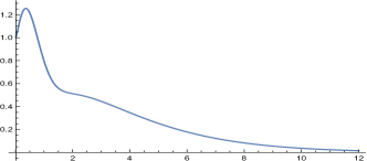
Figure 1: Interpolating function for $f(x)$.

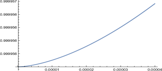
Figure 2: Interpolating function for $f(x)$ with $x$ small.

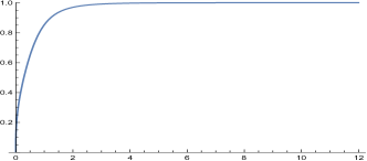
Figure 3: Interpolating function for $\tilde{\rho}(x)$ .

IV Estimates of the (finite) Monopole Energy

In this section we estimate the energy of the monopole solution, as this is of importance for phenomenological searches. Form the theory (10), one may evaluate the stress tensor and from this the total energy of the monopole solution. The latter consists of two parts, the first $E_{1}$ pertains to the kinetic energy of the electromagnetic field (associated with the hypercharge sector) in the non-linear Born-Infeld theory, and the second $E_{2}$ with the non-Abelian SU(2) gauge and Higgs sectors of the theory. In terms of our parametrisation (II), (32) and (33), one has AK

$$E_{\rm total}^{\rm mono} = E_{1}+E_{2},$$

$$E_{1} = 4\pi\,\beta^{2}\,\int_{0}^{\infty}dr\,\left[\sqrt{r^{4}+\frac{1}{(g^{\prime}\,\beta)^{2}}}-r^{2}\right]$$

$$E_{2} = 4\pi\int_{0}^{\infty}dr\left(\frac{1}{g^{2}}\frac{(f^{2}-1)^{2}}{2r^{2}}+\frac{1}{2}\Big{(}r\,\frac{d\rho}{dr}\Big{)}^{2}+\frac{1}{g^{2}}\,\Big{(}\frac{df}{dr}\Big{)}^{2}+\frac{\lambda r^{2}}{8}\left(\rho^{2}-\rho_{0}^{2}\right)^{2}+\frac{1}{4}f^{2}\rho^{2}\right),$$ (60)

where we took into account that in the Born-Infeld hypercharge sector of the monopole solution, only the hypermagnetic field $\vec{{\mathcal{B}}}$ is non-zero (31), implying a Born-Infeld energy $E_{1}=\int 4\pi r^{2}dr(\beta^{2}\sqrt{1+\frac{({\mathcal{B}}^{Y})^{2}}{\beta^{2}}}-\beta^{2})$. The result of the integration in $E_{1}$ can be done analytically by changing integration variable $r=\frac{w}{\sqrt{g^{\prime}\,\beta}}$,  initialBI ; zwiebach and using elliptic integrals:

$$E_{1}=4\pi\,\Big{(}\frac{\beta}{g^{\prime\,3}}\Big{)}^{1/2}\,\int_{0}^{\infty}dw\left[\sqrt{w^{4}+1}-w^{2}\right]=4\pi\,\Big{(}\frac{\beta}{g^{\prime\,3}}\Big{)}^{1/2}\,\frac{(\Gamma(1/4))^{2}}{6\,\sqrt{\pi}}\simeq 15.53\,\Big{(}\frac{\beta}{g^{\prime\,3}}\Big{)}^{1/2}.$$ (61)

From (61) we thus observe that $E_{1}$ is finite for any $\beta<\infty$, as a consequence of the non-linearities of the Born-Infeld sector zwiebach . It was this part that produced the infinities in the energy on the Cho-Maison monopole/dyon solutions CM . Using the SM value $g^{\prime}=0.357$, we then obtain

$$E_{1}\simeq 72.81\sqrt{\beta}.$$ (62)

The quantity $E_{2}$ in (IV) is also finite, and has been finite also in the CM case CM . Using our parametrisation, this quantity can be written as

$${E_{2}} = 4\pi\mu\int_{0}^{\infty}{dx\left[{\frac{{{{\left({{f^{2}}-1}\right)}^{2}}}}{{2{g^{2}}{x^{2}}}}+\frac{{{x^{2}}}}{\lambda}\tilde{\rho}{{}^{\prime\;2}}+\frac{{f{{}^{\prime\;2}}}}{{{g^{2}}}}+\frac{1}{{2\lambda}}{x^{2}}{{\left({{{\tilde{\rho}}^{2}}-1}\right)}^{2}}}+\frac{1}{2\lambda}f^{2}\,\tilde{\rho}^{2}\,\right]},$$ (63)

where the $\prime$ denotes $\frac{d}{dx}$. By inserting our interpolating solutions into (63), and using the values of the parameters of the Standard Model, $g^{\prime}/g={\rm tan}\theta_{W}~{}(\ref{gcoupl}),~{}g^{\prime}=0.357,~{}{\rm sin}^{2}\theta_{W}=0.2312,~{}\rho_{0}\simeq 246.39$ GeV, $\mu=88.39$ GeV, and $\lambda\simeq.26$, we obtain

$$E_{2}=7617~{}{\rm GeV},$$ (64)

which is nearly double (but still of the same order of magnitude as) the value in the CM case CM ; CKY ; AK . The increase in the value of $E_{2}$ is a consequence of the difference of our solution as compared to that of CM, as seen from the figs. 1, 3.

From (62), (64), then, we obtain for the total energy (IV) of the monopole

$$E^{\rm mono}_{\rm total}=(72.81\,\sqrt{\frac{\beta}{(\rm GeV)^{2}}}+7617)~{}{\rm GeV}$$ (65)

In you2 it was argued that the relatively recent measurements of light-by-light scattering by the ATLAS Collaboration hiatl , exploiting Pb-Pb collisions at LHC, imposes a lower bound on the Born-Infeld parameter of the model (10)

$$\sqrt{\beta}\geq 90~{}{\rm GeV}.$$ (66)

From (65) and (66), then, we obtain the following lower bound for the Born-Infeld-Cho-Maison-like monopole mass (=total energy at rest):

$${\mathcal{M}}_{\rm mono}\geq 14.17~{}{\rm TeV}.$$ (67)

Since monopoles are produced in pairs with antimonopoles in colliders, on account of (magnetic) charge conservation, our monopole lies out of the detection range of the LHC , but is of potential relevance to future colliders.

At this stage we stress that $\beta$ is a phenomenological parameter, to be constrained by experiment. However, in the context of microscopic string theory models, though, where the Born-Infeld lagrangian (10) is expected to arise naturally in the low-energy limit, the parameter $\beta\sim M_{s}^{2}$, where $M_{s}$ is the string mass scale. The latter has been constrained by current collider experiments to be at least of ${\mathcal{O}}(10)$ TeV, thus making the term $E_{1}$ (62) dominant over $E_{2}$ in such a case, leading to a significant increase of the monopole mass $E_{\rm total}^{\rm mono}>736$ TeV. Such monopoles could be of cosmological relevance, and be potentially detectable in cosmic monopole searches mitsou (for instance, in future cosmic versions of the MoEDAL experiment). If the monopole masses are in the range $9.3\cdot 10^{3}\,\,{\rm TeV}\leq M_{\rm mono}\,\leq 2.3\cdot 10^{4}\,\,{\rm TeV}$, (with the upper bound associated with constraints on the monopole abundance imposed by Big-Bang nucleosynthesis (BBN)) then according to the analysis in AK , such cosmic monopoles may have interesting consequences for the early universe, including dynamical generation of matter-antimatter asymmetry.

V Conclusions and outlook

In this article, we have discussed some novel semi-analytic (static) monopole solutions in the framework of the phenomenological Lagrangian (10), which constitutes an extension of the SM by a non-linear Born-Infeld Lagrangian for the hypercharge sector only. The solutions we found are consistent with asymptotic analysis for the functions $f(x)$ and $\tilde{\rho}(x)$ characterising the solution (II), but in contrast to the standard Cho-Maison-like CM solutions in the literature AK , they do exhibit some non-monotonic behaviour for $x$ values near $x=0$. This deviation from the standard numerical solutions though is relatively mild, and does not affect the order of magnitude estimates for the total monopole energy, and the associated phenomenology you2 . Nonetheless, from a mathematical point of view our solution is a novel finite-energy monopole solution. Our solutions are analytic, but approximate, as they interpolate between known behaviour for small and large $x$ regions (via appropriate Padé approximants). Establishing the existence of finite energy monopole solutions is important from the experimental point of view, since such solutions can be of relevance for future colliders ( but not the current ones, due to the range of the induced monopole mass which lies outside the capabilities of the LHC ).

Our analysis in this work should be extended to include dyon solutions, carrying both magnetic and electric charge, following the formalism developed in CM ; AK . Since the functions $A(r)$ and $B(r)$, characterising the solution (II), are non-zero the analysis is much more involved than in the monopole case. We leave the study of the dyon case for future work.

Before closing we would like to make an important remark, concerning the finite energy (IV). In the context of the model (10), the Born-Infeld nature of the hypercharge sector decouples from the $SU(2)$ and Higgs sectors, in the sense that the monopole solution is formally the same as that in the SM case of Cho and Maison CM . It is only the non-linear nature of the Born-Infeld energy $E_{1}$ that is finite, and proportional to the parameter $\sqrt{\beta}$, which becomes infinite only in the SM limit $\beta\to\infty$. Finite monopole (solitonic) solutions therefore exist for any value of $\beta$ in this case. However, if one considers effective low-energy field theory models derived from phenomenologically realistic microscopic string theories, then the Born-Infeld non-linear nature is expected to encompass the entire non-Abelian gauge group $SU(2)\times U_{Y}(1)$ and not only the hypercharge $U_{Y}(1)$. In such cases, the gauge and Higgs sectors mix non-trivially with the hypercharge and the resulting monopole/dyon solutions are much more complicated than then solutions considered here and in AK . Moreover, as discussed in silva , in the context of $SU(2)$ Born-Infeld gauge theories, the solitonic monopole/dyon (numerical) solutions exist only for values of the Born-Infeld parameter above a critical value, $\beta\geq\beta_{c}$, estimated numerically in silva , i.e. the energy diverges for $\beta<\beta_{c}$. Although the analysis in silva has been done for simple non-abelian gauge groups $SU(2)$, one expects the above feature to persist in the case where the Born-Infeld sector is extended to include the full standard model non-Abelian group $SU(2)\times U_{Y}(1)$. At present, such a (non-trivial) extension of the analysis of silva is pending. In this respect, however, we should also mention for completeness the model considered in AK2 , according to which two independent Born-Infeld sectors, one for the SU(2) and one for the hypercharge $U_{Y}(1)$ have been considered, with different parameters $\beta_{i}$, $i=1,2$. In the analysis of AK2 , sufficiently large values of the parameter $\beta_{2}$ for the non-Abelian Born-Infeld sector have been implicitly assumed, and in this sense the existence of a critical value of $\beta_{2}^{c}$ cannot be seen. Moreover, this is an effective field theory which is however different from the one in a string theory framework, where the two sectors cannot be separated, and they are both characterised by a common $\beta$. We hope to be able to study in detail monopole/dyon solutions in such realistic string-inspired SM extensions, using our semi-analytic methods, in the future.

Appendix A Coefficients in small-$x$ asymptotic analysis

The $b$ coefficients in (54):

$$b_{11}=-\frac{2b_{01}}{11+10\delta+2\delta^{2}}$$

$$b_{12}=0=b_{14}=b_{15}=b_{16}$$

$$b_{13}=\frac{b_{01}^{3}\left(4\delta^{2}+6\delta+\epsilon\right)}{\delta(2\delta+3)\left(18\delta^{2}+30\delta+11\right)}$$

$$b_{21}=\frac{4b_{01}}{\left(2\delta^{2}+10\delta+11\right)\left(2\delta^{2}+18\delta+39\right)}$$

$$b_{22}=0=b_{24}=b_{26}$$

$$b_{23}=\frac{2b_{01}^{3}\left(-\frac{\epsilon}{\delta(2\delta+3)\left(2\delta^{2}+10\delta+11\right)}-\frac{2\epsilon}{\left(2\delta^{2}+7\delta+5\right)\left(2\delta^{2}+10\delta+11\right)}-\frac{2\left(\frac{\epsilon}{2\delta(2\delta+3)}+1\right)}{18\delta^{2}+30\delta+11}-\frac{6}{2\delta^{2}+10\delta+11}\right)}{3\left(6\delta^{2}+18\delta+13\right)}$$

$$b_{25}=(0.00625575+0.00323926\epsilon+0.00292336\epsilon^{2})b_{01}$$

$$b_{31}=-\frac{8b_{01}}{\left(2\delta^{2}+10\delta+11\right)\left(2\delta^{2}+18\delta+39\right)\left(2\delta^{2}+26\delta+83\right)}$$

$$b_{32}=0=b_{34}=b_{36}$$

$$b_{33}=(0.0015303+0.00014715\epsilon)b_{01}^{3}$$

$$b_{35}=(-0.00174278-0.00067203\epsilon-0.000413624\epsilon^{2})b_{01}^{5}$$

$$b_{41}=1.61775\times 10^{-6}b_{01}$$

$$b_{42}=0=b_{44}=b_{46}$$

$$b_{43}=(-0.0000986062-4.70038\times 10^{-6}\epsilon)b_{01}^{3}$$

$$b_{45}=(0.000248585+0.00007087280\epsilon+.000030011\varepsilon^{2})b_{01}^{5}$$

$$b_{51}=-1.37892\times 10^{-8}b_{01}$$

$$b_{52}=0=b_{54}=b_{56}$$

$$b_{53}=(4.64828\times 10^{-6}+1.24034\times 10^{-7}\epsilon)b_{01}^{3}$$

$$b_{55}=(-0.0000239827-4.97425\times 10^{-6}\epsilon-1.5915\times 10^{-6}\epsilon^{2})b_{01}^{5}$$

$$b_{61}=8.368\times 10^{-11}b_{01}$$

$$b_{62}=0=b_{64}=b_{66}$$

$$b_{63}=-(1.67851\times 10^{-7}+2.86179\times 10^{-9}\epsilon)b_{01}^{3}$$

$$b_{65}=(1.74488\times 10^{-6}+2.5867\times 10^{-7}\epsilon+6.95189\times 10^{-8}\epsilon^{2})b_{01}^{5}$$

We will now list the ’a’ coefficients in (53):

$$a_{12}=\epsilon b_{01}^{2}/(2\delta(3+2\delta))$$

$$a_{13}=0=a_{14}=a_{15}=a_{16}$$

$$a_{22}=-2\epsilon b_{01}^{2}/((5+7\delta+2\delta^{2})(11+10\delta+2\delta^{2}))$$

$$a_{23}=0=a_{25}=a_{26}$$

$$a_{24}=(0.00732333\epsilon+0.0369758\epsilon^{2})b_{01}^{4}$$

$$a_{32}=0.000809972\epsilon b_{01}^{2}$$

$$a_{33}=0=a_{35}=a_{36}$$

$$a_{34}=-(0.00115918\epsilon+0.00361289\epsilon^{2})b_{01}^{4}$$

$$a_{42}=-0.0000277424\epsilon b_{01}^{2}$$

$$a_{43}=0=a_{45}$$

$$a_{44}=(0.000105727\epsilon+0.000261013\epsilon^{2})b_{01}^{4}$$

$$a_{46}=-(0.0000845209\epsilon+0.000354434\epsilon^{2}+0.000438062\epsilon^{3})b_{01}^{6}$$

$$a_{52}=6.94301\times 10^{-7}\epsilon b_{01}^{2}$$

$$a_{53}=0=a_{55}$$

$$a_{54}=-(6.89031\times 10^{-6}\epsilon+0.0000140244\epsilon^{2})b_{01}^{4}$$

$$a_{56}=(0.0000114343\epsilon+0.0000421252\epsilon^{2}+0.0000383327\epsilon^{3})b_{01}^{6}$$

$$a_{62}=-1.31163\times 10^{-8}\epsilon b_{01}^{2}$$

$$a_{63}=0=a_{65}$$

$$a_{64}=(3.4889\times 10^{-7}\epsilon+6.014\times 10^{-7}\epsilon^{2})b_{01}^{4}$$

$$a_{66}=-(1.0851\times 10^{-6}\epsilon+2.57347\times 10^{-6}\epsilon^{3}+3.56687\times 10^{-6}\epsilon^{2})b_{01}^{6}$$

References

• (1) S. Arunasalam and A. Kobakhidze, “Electroweak monopoles and the electroweak phase transition,” Eur. Phys. J. C 77, no. 7 (2017), 444 doi:10.1140/epjc/s10052-017-4999-y [arXiv:1702.04068 [hep-ph]].
• (2) Y. M. Cho and D. Maison, “Monopoles in Weinberg-Salam model,” Phys. Lett. B 391 (1997), 360 doi:10.1016/S0370-2693(96)01492-X [hep-th/9601028].
• (3) P. A. M. Dirac, “Quantised singularities in the electromagnetic field,,” Proc. Roy. Soc. Lond. A 133 (1931) no.821, 60. doi:10.1098/rspa.1931.0130
• (4) G. ’t Hooft, “Magnetic Monopoles in Unified Gauge Theories,” Nucl. Phys. B 79 (1974), 276 . doi:10.1016/0550-3213(74)90486-6; A. M. Polyakov, “Particle Spectrum in the Quantum Field Theory,” JETP Lett.  20 (1974), 194 [Pisma Zh. Eksp. Teor. Fiz.  20 (1974), 430 ].
• (5) Y. M. Cho, K. Kim and J. H. Yoon, “Finite Energy Electroweak Dyon,” Eur. Phys. J. C 75, no. 2 (2015) 67 doi:10.1140/epjc/s10052-015-3290-3 [arXiv:1305.1699 [hep-ph]].
• (6) J. Ellis, N. E. Mavromatos and T. You, “The Price of an Electroweak Monopole,” Phys. Lett. B 756 (2016) 29 doi:10.1016/j.physletb.2016.02.048 [arXiv:1602.01745 [hep-ph]].
• (7) M. B. Green, J. H. Schwarz and E. Witten, “Superstring Theory. Vols. 1: Introduction,” Cambridge, Uk: Univ. Pr. ( 1987) 469 P. ( Cambridge Monographs On Mathematical Physics); “Superstring Theory. Vol. 2: Loop Amplitudes, Anomalies And Phenomenology,” Cambridge, Uk: Univ. Pr. ( 1987) 596 P. ( Cambridge Monographs On Mathematical Physics).
• (8) H. Kim, “Genuine dyons in Born-Infeld electrodynamics,” Phys. Rev. D 61 (2000) 085014 doi:10.1103/PhysRevD.61.085014 [hep-th/9910261].
• (9) See, for instance: B. Zwiebach, “A first course in string theory,” (Cambridge, UK: Univ. Pr. (2009)), and references therein.
• (10) V. Vento, “Ions, Protons, and Photons as Signatures of Monopoles,” Universe 4 (2018) no.11, 117. doi:10.3390/universe4110117, and references therein.
• (11) G. Aad et al. [ATLAS Collaboration], “Search for magnetic monopoles and stable particles with high electric charges in 8 TeV $pp$ collisions with the ATLAS detector,” Phys. Rev. D 93 (2016) no.5, 052009 doi:10.1103/PhysRevD.93.052009 [arXiv:1509.08059 [hep-ex]].
• (12) B. Acharya et al. [MoEDAL Collaboration], “Search for magnetic monopoles with the MoEDAL forward trapping detector in 2.11 fb-1 of 13 TeV proton-proton collisions at the LHC,” Phys. Lett. B 782 (2018) 510 doi:10.1016/j.physletb.2018.05.069 [arXiv:1712.09849 [hep-ex]]. B. Acharya et al. [MoEDAL Collaboration], “The Physics Programme Of The MoEDAL Experiment At The LHC,” Int. J. Mod. Phys. A 29 (2014) 1430050 doi:10.1142/S0217751X14300506 [arXiv:1405.7662 [hep-ph]].
• (13) A. K. Drukier and S. Nussinov, “Monopole Pair Creation in Energetic Collisions: Is It Possible?,” Phys. Rev. Lett.  49 (1982) 102. doi:10.1103/PhysRevLett.49.102
• (14) O. Gould and A. Rajantie, “Thermal Schwinger pair production at arbitrary coupling,” Phys. Rev. D 96 (2017) no.7, 076002 doi:10.1103/PhysRevD.96.076002 [arXiv:1704.04801 [hep-th]].
• (15) O. Gould and A. Rajantie, “Magnetic monopole mass bounds from heavy ion collisions and neutron stars,” Phys. Rev. Lett.  119 (2017) no.24, 241601 doi:10.1103/PhysRevLett.119.241601 [arXiv:1705.07052 [hep-ph]].
• (16) J. Ellis, N. E. Mavromatos and T. You, “Light-by-Light Scattering Constraint on Born-Infeld Theory,” Phys. Rev. Lett.  118 (2017) no.26, 261802 doi:10.1103/PhysRevLett.118.261802 [arXiv:1703.08450 [hep-ph]].
• (17) Annie A.M. Cuyt, ”A review of multivariate Padé approximation theory” Journal of Computational and Applied Mathematics Vol 12 and 13 (1985) , 221.
• (18) G. A. Baker ”Essentials of Padé approximations” Academic, London, 1975.
• (19) M. Aaboud et al. [ATLAS Collaboration], “Evidence for light-by-light scattering in heavy-ion collisions with the ATLAS detector at the LHC,” Nature Phys.  13 (2017) no.9, 852 doi:10.1038/nphys4208 [arXiv:1702.01625 [hep-ex]]; see also: D. d’Enterria and G. G. da Silveira, “Observing light-by-light scattering at the Large Hadron Collider,” Phys. Rev. Lett.  111 (2013) 080405 Erratum: [Phys. Rev. Lett.  116 (2016) no.12, 129901] doi:10.1103/PhysRevLett.111.080405, 10.1103/PhysRevLett.116.129901 [arXiv:1305.7142 [hep-ph]].
• (20) V. A. Mitsou, “The quest for magnetic monopoles ? past, present and future,” PoS CORFU 2017 (2018) 188. doi:10.22323/1.318.0188, and references therein.
• (21) N. E. Grandi, A. Pakman, F. A. Schaposnik and G. A. Silva, “Monopoles, dyons and theta term in Dirac-Born-Infeld theory,” Phys. Rev. D 60 (1999) 125002 doi:10.1103/PhysRevD.60.125002 [hep-th/9906244].
• (22) S. Arunasalam, D. Collison and A. Kobakhidze, “Electroweak monopoles and electroweak baryogenesis,” arXiv:1810.10696 [hep-ph].