Towards a More Practice-Aware Runtime Analysis of Evolutionary Algorithms

Abstract

Theory of evolutionary computation (EC) aims at providing mathematically founded statements about the performance of evolutionary algorithms (EAs). The predominant topic in this research domain is runtime analysis, which studies the time it takes a given EA to solve a given optimization problem. Runtime analysis has witnessed significant advances in the last couple of years, allowing us to compute precise runtime estimates for several EAs and several problems.

Runtime analysis is, however (and unfortunately!), often judged by practitioners to be of little relevance for real applications of EAs. Several reasons for this claim exist. We address two of them in this present work: (1) EA implementations often differ from their vanilla pseudocode description, which, in turn, typically form the basis for runtime analysis. To close the resulting gap between empirically observed and theoretically derived performance estimates, we therefore suggest to take this discrepancy into account in the mathematical analysis and to adjust, for example, the cost assigned to the evaluation of search points that equal one of their direct parents (provided that this is easy to verify as is the case in almost all standard EAs). (2) Most runtime analysis results make statements about the expected time to reach an optimal solution (and possibly the distribution of this optimization time) only, thus explicitly or implicitly neglecting the importance of understanding how the function values evolve over time. We suggest to extend runtime statements to runtime profiles, covering the expected time needed to reach points of intermediate fitness values.

While certainly other reasons exist to believe that runtime analysis is of limited practical relevance, and while our suggested solutions can only serve as a pointer to a more practice-aware runtime analysis theory, we are confident that our work helps to initiate a more constructive exchange between theoretical and empirically-driven research in EC.

As a more direct consequence, we obtain a result showing that the greedy (2+1) GA of Sudholt [GECCO 2012] outperforms any unary unbiased black-box algorithm on OneMax, thus giving strong evidence that our suggested performance measure has the potential to drastically change the theoreticians’ view on long-standing hypotheses in evolutionary computation.

1 Introduction

Evolutionary algorithms (EAs) are bio-inspired black-box optimization heuristics that are successfully applied to a broad range of industrial and academic optimization problems. Their practical relevance has motivated theoreticians to analyze EAs by mathematically means, aiming at providing mathematically founded insights into the working principles of EAs. Unfortunately, we see today a rather big gap between theoretical and practice-driven research in evolutionary computation (EC). Unlike in classical computer science, where a fruitful interplay between mathematically- and empirically-driven research exists, theory of EAs is regularly considered “useless” in the more practically-oriented part of the EC research community, cf., e.g., Footnote 4 in [EHM99], where it is stated that “the best thing a practitioner of EA’s can do is to stay away from theoretical results”. One critical reason for such claims is the fact that EAs are particularly useful when the problem at hand is not analyzable by thorough mathematical means; while for problems that do admit such a mathematical approach, problem-tailored algorithms are typically much more powerful than heuristics. This gap is very difficult, if not impossible, to close. At the same time, however, we also see that some of the other reasons for practitioners not to follow too closely what theory of EC can offer could be easily addressed. We suggest in this work two different steps in this direction, i.e., towards a more practice-aware theory of EAs. Our hope is to trigger with this work a more constructive exchange between theoretical and empirical research streams in EC.

As a side effect of our work, we also obtain some theoretical results that are interesting in their own rights. We summarize our proposed changes and results in Sections 1.1 and 1.2.

1.1 Implementation-Aware Runtime Analysis

The by-far most relevant performance measure in discrete black-box optimization is the number of fitness evaluations that an algorithm needs until it evaluates for the first time an optimal search point. This runtime (also: optimization time) measure is often motivated by the fact that in typical applications the function evaluations are the most costly part of the black-box optimizer. Another motivation for this performance measure is the fact that black-box optimizers are often used in situations where the data is subject to privacy concerns, so that the data owner will be able to answer individual function evaluation requests but does not or cannot reveal any other information about its data. Counting function evaluations is a standard complexity measure both in EC but also in classical computer science, where it is studied under the notion of query complexity.

One seemingly negligible difference between the runtime studied in the theory of EAs and that studied in practice- or empirically-motivated work is the fact that in most theory works function evaluations are counted also for iterations in which the offspring equals its parent (or one of its parents in case of recombination). In many EAs this situation occurs frequently. For example, when using standard bit mutation (cf. Section 2 for a description of the here-mentioned variation operators, algorithms, and problem classes) with mutation rate $p=1/n$, the probability that the mutated offspring equals its parent is $(1-p)^{n}\approx 1/e=0.368$, showing that, for example, the $(1+1)$ EA, which only uses standard bit mutation as variation operator, uses a $1/e$ fraction of its function evaluations for offspring that are identical to the parent. In practical implementations one would of course avoid such evaluations, in particular when it is easy to check (as in this case) that the offspring equals its parent.

A similar situation, in which the offspring is likely to equal one of its parents, occurs when two similar parents are recombined. This is quite frequent in typical $(\mu+\lambda)$ GAs. Furthermore, a biased crossover favoring entries from one of the parents as, for example, used in the $(1+(\lambda,\lambda))$ GA proposed in [DDE15], has a relatively high probability to reproduce one of the parent solutions even if the Hamming distance of the two parents is large. Since in these cases it is typically quite easy to determine if the recombined offspring equals one of its parents, the offspring would not be evaluated in typical implementations, while in existing theoretical runtime analysis statements we would charge the algorithm one function evaluation for creating this offspring.

These discrepancies between the analyzed and the actually implemented EAs can result in significant gaps between empirically observed and mathematically derived performance estimates. To reduce this gap, we suggest to reflect these observations in the runtime bounds, by analyzing EA variants in which offspring are not evaluated if they equal one of their parents and this equality is easy to determine. In the case of standard bit mutation, two straightforward ways to implement this strategy exist. The first one simply ignores such iterations, thus effectively resampling an offspring until it differs from its parent. This strategy can be efficiently implemented by sampling the mutated offspring from a conditional distribution. The second idea is to flip one random bit in case no bit is flipped in the mutation step (thus effectively shifting the probability mass to flip zero bits to the probability to flip exactly one bit). In the case of crossover there are many ways to deal with such situations. When crossover is followed by mutation, we suggest to use one of the just-mentioned two solutions to ensure flipping at least one bit in the mutation step if the offspring created by recombination is merely a copy of one of its parents. When crossover is not followed by mutation (as in the $(1+(\lambda,\lambda))$ GA), we suggest to simply omit the function evaluation of such offspring.

We analyze in Sections 2.1 and 2.2 how these suggestions influence the performances of the $(1+1)$ EA, the $(1+(\lambda,\lambda))$ GA proposed in [DDE15], and the Greedy $(2+1)$ GA from [Sud12]. While the theoretical bounds are easy to obtain, we observe a quite surprising result. We show in Theorem 15 that our simple modification of the Greedy $(2+1)$ GA yields a better expected optimization time on OneMax than any unary unbiased (i.e., mutation-based) black-box algorithm. As far as we know, this shows for the first time that a classical genetic algorithm with crossover can outperform all unary unbiased black-box algorithms on the simple hill climbing problem OneMax. Given the long series of works trying to establish such results (cf. the literature surveys in [DDE15, Sud12]), this shows that our simple suggestion of a more implementation-aware runtime analysis can have substantial impact on the theoretician’s view on some of the most fundamental questions in EC.

We note that previous attempts to establish more meaningful complexity measures in EC exists, most notably in the work of Jansen and Zarges [JZ11], who propose to profile how much time is spend in each of the steps of an EA relative to the cost of the function evaluation. Jansen and Zarges also briefly discuss the here-proposed resampling variant of the $(1+1)$ EA, but conclude from their work that “the simple cost model [of not counting mutation steps of the $(1+1)$ EA in which no bit is flipped] is inadequate”. We do agree that counting function evaluations may not always reflect very well the wall-clock time spend on a problem (in particular if Hash-tables are used to achieve the already evaluated search points or if evaluation can be done in constant time for offspring resembling previously evaluated ones). It is still, as mentioned above, the most relevant cost measure in EC. The research question that we address in this work is how to deal with offspring that equal their parents, and our suggestion is to adopt a more implementation-aware view in runtime analysis.

1.2 Runtime Profiles

Our second suggestion concerns the problem that in most theoretical works on EAs for discrete optimization problems, only the expected times to hit an optimal solution for the first time are reported. In realistic environments, we do not know when this is the case, making it equally important to understand how the fitness values evolve over time. We therefore introduce in Section 3 the concept of runtime profiles, the expected time needed to hit intermediate target values. In the case of OneMax or LeadingOnes functions of dimension $n$, these runtime profiles could be the expected times to reach any fitness level $i\in[n]$, while for problems taking less canonical fitness values, other intermediate target values could be used. In short, our suggestion is to state runtime profiles of an algorithm rather than only the optimization time.

As we shall discuss in Section 3, it is quite interesting to observe how the first hitting times for the different targets evolve. Already for the simple LeadingOnes benchmark functions we see that the $(1+1)$ EA-variants proposed in Section 2.1 are superior to RLS for all target fitness values $i$ that are smaller than some relatively large threshold value $v$, while RLS reaches fitness levels $i\geq v$ faster than the $(1+1)$ EA-counterparts. Reporting only the expected optimization time therefore does not do justice to the better performance of the $(1+1)$ EA-variants in the earlier parts of the optimization process.

We are confident that the proposed runtime profiles will be very useful for the design and the analysis of non-static parameter and operator choices in EAs, such as adaptive mutation or crossover rates, selection pressure, etc. This topic, also studied under the notions of hyper-heuristics, meta-heuristics, etc., has very recently seen increased interest in the theory of EC community [DD15a, DDY16a, DDK16, DL16]. It is a highly relevant topic in empirically-driven research in EC, cf. [AM16, EHM99, EMSS07, KHE15] and references therein.

Our runtime profiles complement the fixed-budget perspective proposed in [JZ14], where statements about the expected fitness values after a fixed number of fitness evaluations are sought. Runtime profiles and fixed-budget perspectives are orthogonal views on the performance of EAs, both aiming at providing more insight into the optimization behavior than what the single runtime measure can offer. Neither of these two measures is entirely new but rather summarize performance statements frequently reported in empirical works. The aim of [JZ14] as well as our own work is to motivate researchers working in the theory of EC to include in their statements these more informative performance guarantees.

Complexity of Implementing Our Suggestions. We emphasize that from a theoretical point of view all our suggestions are easy to implement. Indeed, all results reported in this work can be easily derived from existing runtime results. But, as our result for the Greedy $(2+1)$ GA${}_{\text{mod}}$ shows, it may drastically change our view on classical EAs.

Appendix. Detailed experimental data for the figures reported in the main file as well as some technical statements needed in our proofs are reported in the appendix.

2 Implementation-Aware Runtime Analysis

Standard implementations of EAs often differ from their vanilla pseudocode descriptions. These “tweaks” are either strictly needed to make an algorithmic idea implementable or just “nice to have”, in order to speed up an algorithm without changing its performance. In this section, we describe some of such typical differences, and analyze their impact on standard runtime results in EC.

Scope: In the following, we consider the maximization of single-objective pseudo-Boolean functions $f:\{0,1\}^{n}\rightarrow\mathbb{R}$, but all our suggestion can be applied to other search and objective spaces.

Notation: We use $n$ to denote the problem dimension. We abbreviate $[n]:=\{1,2,\ldots,n\}$ and $[0..n]:=\{0\}\cup[n]$. By $\ln$ we denote the natural logarithm to base $e:=\exp(1)$. For every positive integer $d$ we denote by $H_{d}$ the $d$-th harmonic number $H_{d}:=\sum_{i=1}^{d}{1/i}=\ln(d)+\gamma+O(1/d)$ with $\gamma\approx 0.5772156649$ being the Euler–Mascheroni constant.

2.1 The (1+1) EA

One of the best-studied EAs in the theory of EC is the $(1+1)$ EA. It has a simple structure and is often used as a showcase to understand the role of global mutation in combination with elitist selection.

The $(1+1)$ EA works as follows. It has a very restricted memory (“population”), keeping only the best so-far solution candidate in the memory (and the most recent one in case several search points of current-best function value have been evaluated). In the mutation step, an offspring $y$ is sampled from this current-best solution $x$ by changing each bit in $x$ with some mutation probability $p\in(0,1)$, independently of all other bits. In the selection step, the parent $x$ is replaced by its offspring $y$ if and only if the fitness of $y$ is at least as good as the one of $x$; i.e., in the case of maximization, if and only if $f(y)\geq f(x)$.

When implementing the $(1+1)$ EA, it would be inconvenient and time-consuming to sample in each iteration and for each bit the random Bernoulli variable describing whether or not the corresponding bit should be flipped. A common way to implement the standard bit mutation is to sample in the beginning of the mutation step a random variable $\ell$ from the binomial distribution $\operatorname{Bin}(n,p)$ with $n$ trials and success probability $p$, i.e., $\mathbb{P}[\ell=k]=\binom{n}{k}p^{k}(1-p)^{n-k}$ for all $k\in[0..n]$. Once $\ell$ is sampled, $\ell$ different (i.e., without replacement) positions $i_{1},\ldots,i_{\ell}\in[n]$ are chosen uniformly at random and $y$ is created from $x$ by copying $y_{i}:=x_{i}$ for $i\in[n]\setminus\{i_{1},\ldots,i_{\ell}\}$ and setting $y_{i}:=1-x_{i}$ for $i\in\{i_{1},\ldots,i_{\ell}\}$. It is not difficult to verify that this implementation is identical to the one with $n$ independent Bernoulli trials.

This way, the $(1+1)$ EA can be stated in the form of Algorithm 1. Note here that no termination criterion is specified. This is justified by the fact that runtime analysis studies the expected time this algorithm needs to find an optimal solution. In real implementations, of course, one has to specify a termination criterion, which can be, for example, an upper bound on the number of iterations, on CPU time, or the number of iterations in which no improvement has been observed, but also the first point in time a certain fitness-value has been reached, etc.

1Initialization: Sample $x\in\{0,1\}^{n}$ uniformly at random and compute $f(x)$;

2 Optimization: for $t=1,2,3,\ldots$ do

3       Sample $\ell\sim\operatorname{Bin}(n,p)$;

4       $y\leftarrow\operatorname{mut}_{\ell}(x)$;

5       evaluate $f(y)$;

6       if $f(y)\geq f(x)$ then $x\leftarrow y$;

7      

Algorithm 1 (The well-known $(1+1)$ EA with mutation probability $p\in(0,1)$ for the maximization of a pseudo-Boolean function $f:\{0,1\}^{n}\rightarrow\mathbb{R}$).

1Input: $x\in\{0,1\}^{n}$, $\ell\in\mathbb{N}$;

2 Select $\ell$ different positions $i_{1},\ldots,i_{\ell}\in[n]$ u.a.r.;

3 $y\leftarrow x$;

4 for $j=1,...,\ell$ do $y_{i_{j}}\leftarrow 1-x_{i_{j}}$;

Algorithm 2 ($\operatorname{mut}_{\ell}$ chooses $\ell$ different positions and flips the entries in these positions.).

Implementing the Bernoulli trials of the standard bit mutation as above did not affect the performance of the $(1+1)$ EA. But there is another tweak that can speed up the algorithm significantly. The idea is simple and therefore found in most standard implementations of the $(1+1)$ EA. The probability that $\ell$ in line 1 of Algorithm 1 equals zero is $(1-p)^{n}$. For the often recommended choice $p=1/n$ this results in a $1/e$ fraction of iterations in which no bit is flipped at all. In the vanilla description of the $(1+1)$ EA above, we would still count one function evaluation for any of these iterations (cf. line 1). In practice, however, we would rather ignore such iterations by (1) either re-sampling $\ell$ until we sample a value $\ell>0$ (this is the case if we simply skip line 1 in Algorithm 1 whenever $\ell=0$) or (2) by using $\ell=1$ if $\ell=0$ is sampled. We refer to the $(1+1)$ EA using the first option as $(1+1)$ EA_>0 (“resampling EA”, Algorithm 3), and we call the algorithm using the second option the $(1+1)$ EA_0→1 (“shift EA”, Algorithm 4). The $(1+1)$ EA_>0 can efficiently be implemented by sampling $\ell$ from the conditional distribution $\operatorname{Bin}_{>0}(n,p)$, which assigns to each $k$ a probability of $\mathbb{P}[\ell=k|\ell>0]=\binom{n}{k}p^{k}(1-p)^{n-k}/(1-(1-p)^{n})$.

1Initialization: Sample $x\in\{0,1\}^{n}$ uniformly at random and compute $f(x)$;

2 Optimization: for $t=1,2,3,\ldots$ do

3       Sample $\ell\sim\operatorname{Bin}_{>0}(n,p)$;

4       $y\leftarrow\operatorname{mut}_{\ell}(x)$;

5       evaluate $f(y)$;

6       if $f(y)\geq f(x)$ then $x\leftarrow y$;

7      

Algorithm 3 (The $(1+1)$ EA_>0 with mutation probability $p\in(0,1)$ for the maximization of a pseudo-Boolean function $f:\{0,1\}^{n}\rightarrow\mathbb{R}$).

1Initialization: Sample $x\in\{0,1\}^{n}$ uniformly at random and compute $f(x)$;

2 Optimization: for $t=1,2,3,\ldots$ do

3       Sample $\ell\sim\operatorname{Bin}(n,p)$;

4       if $\ell=0$ then $\ell\leftarrow 1$;

5       $y\leftarrow\operatorname{mut}_{\ell}(x)$;

6       evaluate $f(y)$;

7       if $f(y)\geq f(x)$ then $x\leftarrow y$;

8      

Algorithm 4 (The $(1+1)$ EA_0→1 with standard mutation probability $p\in(0,1)$ for the maximization of a pseudo-Boolean function $f:\{0,1\}^{n}\rightarrow\mathbb{R}$).

In the next two subsections, we discuss how these strategies change the expected optimization time of the $(1+1)$ EA on OneMax (Sec. 2.1.1) and on LeadingOnes (Sec. 2.1.3), respectively. We refer the interested reader to Section A in the appendix for a discussion of the regarded benchmark problems.

2.1.1 Performance of the (1+1) EA Variants on OneMax

We start our investigations by regarding OneMax, the best-understood benchmark problem in runtime analysis. OneMax is the function that returns as function value the number of ones in a string, i.e., $\textsc{Om}(x):=\sum_{i=1}^{n}{x_{i}}$. We compare the performance of the $(1+1)$ EA, the $(1+1)$ EA_>0, and the $(1+1)$ EA_0→1. We also add to our experiments a comparison with Randomized Local Search (RLS), the standard first-ascent hill climber which samples in each iteration a random neighbor at Hamming distance 1 from the current-best solution. We obtain RLS from Algorithm 1 by replacing line 1 with “Set $\ell=1$;”.

From a mathematical point of view, the suggested changes do not cause much trouble. In fact, the runtime behavior of the $(1+1)$ EA on OneMax (cf. [HPR⁺14] and references mentioned therein) and, more generally, linear functions $f:\{0,1\}^{n}\rightarrow\mathbb{R},x\mapsto\sum_{i=1}^{n}{w_{i}x_{i}}$ with $w_{i}\in\mathbb{R}$ [Wit13] is quite well understood. The following result easily follow from standard fitness level arguments and illustrates how existing runtime results for the $(1+1)$ EA can easily be adapted to the $(1+1)$ EA_>0 and the $(1+1)$ EA_0→1.

Theorem 5.

The expected optimization time of the $(1+1)$ EA_>0 with mutation probability $p\in(0,1)$ for OneMax is at most $\frac{1-\left(1-p\right)^{n}}{p\left(1-p\right)^{n-1}}H_{n}$ and for the $(1+1)$ EA_0→1 it is at most $\frac{1}{(1-p)^{n-1}(np+1-p)}nH_{n}$.

Proof of the upper bound for the $(1+1)$ EA_>0 on OneMax in Theorem 5.

We do a simple fitness level argument, using the canonical fitness level partition $L_{0},L_{1},\ldots,L_{n}$ with $L_{i}:=\{x\in\{0,1\}^{n}\mid\textsc{Om}(x)=i\}$.

For $i\in\{0,\dots,n-1\}$ let $p_{i}$ be the probability to leave fitness level $L_{i}$ in one iteration of the $(1+1)$ EA_>0 with mutation probability $p$ when starting in some $x\in L_{i}$. Since the fitness $L_{i}$ is left if one of the $(n-i)$ 0-bits and no other bit is flipped, we can bound $p_{i}$ from below as

$$p_{i}\geq\frac{\binom{n-i}{1}p\left(1-p\right)^{n-1}}{1-\left(1-p\right)^{n}},$$

using that the probability to sample $\ell=1$ in line 3 of Algorithm 3 is $p\left(1-p\right)^{n-1}/(1-\left(1-p\right)^{n})$. Summing up the expected waiting times $1/p_{i}$, we thus get

$$\mathbb{E}[T_{>0,p}(\textsc{Om})] \leq\sum\limits_{i=0}^{n-1}\frac{1}{p_{i}}\leq\sum\limits_{i=0}^{n-1}\left(1-\left(1-p\right)^{n}\right)\frac{1}{n-i}\frac{1}{p\left(1-p\right)^{n-1}}\leq\frac{\left(1-\left(1-p\right)^{n}\right)}{p(1-p)^{n-1}}H_{n}.$$

∎

The proof for the $(1+1)$ EA_0→1 is very similar.

Proof of the upper bound for the $(1+1)$ EA_0→1 on OneMax in Theorem 5.

We use the same fitness level partition as for the $(1+1)$ EA_>0. Letting $p_{i}$ be the probability to leave fitness level $L_{i}$ in one iteration of the $(1+1)$ EA_0→1 with mutation probability $p$ when starting in some $x\in L_{i}$, we bound

$$p_{i} \geq\binom{n-i}{1}p\left(1-p\right)^{n-1}+\frac{n-i}{n}(1-p)^{n}$$

$$\geq(1-p)^{n-1}\left((n-i)p+\frac{n-i}{n}(1-p)\right)$$

$$\geq(1-p)^{n-1}(np+1-p)\frac{n-i}{n}.$$

Summing up expected waiting times $1/p_{i}$ yields

$$\mathbb{E}[T_{\operatorname{0\rightarrow 1},p}(\textsc{Om})] \leq\frac{1}{(1-p)^{n-1}(np+1-p)}\sum\limits_{i=0}^{n-1}\frac{n}{n-i}\leq\frac{1}{(1-p)^{n-1}(np+1-p)}nH_{n}.$$

∎

For the most often recommended choice $p=1/n$, the expected optimization time of the $(1+1)$ EA equals $en\ln(n)-1.8925...n+\tfrac{e}{2}\ln(n)+0.5978...+O(\log n/n)$ [HPR⁺14], while the bounds in Theorem 5 evaluate to $(e-1+\tfrac{1}{n})nH_{n}\approx 1.718n\ln(n)+0.918n+\ln(n)+O(1)$ for the $(1+1)$ EA_>0 and $\frac{e}{2-1/n}nH_{n}\approx 1.3591n\ln(n)+0.7845n+O(1)$ for the $(1+1)$ EA_0→1. For this choice of $p$, the bound for the $(1+1)$ EA_>0 is tight, as the following theorem shows.

Theorem 6.

Let $p=O(n^{-2/3-\varepsilon})$. Then the expected time of the $(1+1)$ EA_>0 with mutation probability $p$ on OneMax bounded from below by

$$(1-o(1))\frac{1-(1-p)^{n}}{p(1-p)^{n}}\min\{\ln n,\ln(1/(p^{3}n^{2}))\}.$$

In particular, for any constant $c>0$, the expected runtime of the $(1+1)$ EA_>0 with mutation probability $p=c/n$ on OneMax is at least $(1-o(1))\frac{e^{c}-1}{c}n\ln n$.

Our proof of Theorem 6 follows very closely that of Theorem 6.5 in [Wit13]. Note that Witt actually proves a lower bound for what he calls “arbitrary mutation-based EAs” or “(1+1) EA_μ”, i.e., EAs using as starting point the best out of $\mu$ search points drawn independently and uniformly at random and then using standard bit mutation as only means of variation. Our statement also holds for this larger class of algorithms, i.e., the class of all (1+1) EA_μ,>0 not evaluating offspring that equal their immediate parent.

A useful tool in his analysis is the following drift theorem, also proven in [Wit13].

Theorem 7 (Multiplicative Drift Lower Bound from [Wit13]).

Let $S\subseteq\mathbb{R}$ be a finite set of positive numbers with minimum 1. Let $\{X^{(t)}\}_{t\geq 0}$ be a sequence of random variables over $S$, where $X^{(t+1)}\leq X^{(t)}$ for any $t\geq 0$ and let $s_{\min}>0$. Let $T$ be the random variable that gives the first in point time $t\geq 0$ for which $X^{(t)}\leq s_{\min}$. If there exist positive reals $\beta,\delta\leq 1$ such that, for all $s>s_{\min}$ and all $t\geq 0$ with $\mathbb{P}(X^{(t)}=s)>0$,

1. $\mathbb{E}[X^{(t)}-X^{(t+1)}|X^{(t)}=s]\leq\delta s$,

2. $\mathbb{P}(X^{(t)}-X^{(t+1)}\geq\beta s|X^{(t)}=s)\leq\beta\delta/\ln s$,

then for all $s_{0}\in S$ with $\mathbb{P}(X^{(0)}=s_{0})>0$,

$$\mathbb{E}[T|X^{(0)}=s_{0}]\geq\frac{\ln(s_{0})-\ln(s_{\min})}{\delta}\frac{1-\beta}{1+\beta}.$$

As a first step towards a proof of Theorem 6, we state the following bound on the expected progress, which follows directly from Lemma 6.7 in [Wit13], just taking into account that the $(1+1)$ EA_>0 does not sample $0$.

Lemma 8.

Consider the $(1+1)$ EA_>0 with mutation probability $p$ for the maximization of OneMax. Given a current search point with $i$ 0-bits, let $I^{\prime}$ denote the number of 0-bits in the subsequent search point (after selection). Then we have $\mathbb{E}(i-I^{\prime})\leq\frac{ip}{1-(1-p)^{n}}\left(1-p+\frac{ip^{2}}{1-p}\right)^{n-1}$.

Along with the multiplicative drift lower bound theorem (repeated here as Theorem 7), Theorem 6 can now be proven as follows.

Proof.

As mentioned above, we follow very closely the proof of Theorem 6.5 in [Wit13]. We also use the same notation, just changing the meaning of 0- and 1-bits as Witt considers minimization whereas we regard the maximization. This only has an influence on the notation, not on any of the statements. Using the fact that OneMax is the easiest to optimize pseudo-Boolean linear function (cf. [DJW12], the proof easily carries over to the $(1+1)$ EA_>0), it suffices to prove the claimed lower bound for OneMax.

Let $X^{(t)}$ be the number of 0-bits in the solution at time $t$ and let $\tilde{p}=\max\{p,1/n\}$. The probability of flipping at least $b=\tilde{p}n\ln n$ bit is superpolynomially small. We can therefore condition on this event not happening in any of the first $n^{2}$ iterations and pessimistically assume that the runtime of the $(1+1)$ EA_>0 is $0$ whenever $b$ or more bits are flipped in the first $n^{2}$ iterations.

As in [Wit13] it is not difficult to argue that with probability $1-o(1)$ the $(1+1)$ EA_>0 reaches a state in which the search point in the memory has between $s_{\max}/2$ and $s_{\max}:=1/(2n\tilde{p}^{2}\ln n)$ 0-bits. Let $t^{*}$ be the first point in time that this happens. We bound from below the time needed by the $(1+1)$ EA_>0 to reach, starting in the current search point $x^{(t^{*})}$ having at most $s_{\max}$ 0-bits, a search point having at most $s_{\min}:=n\tilde{p}\ln^{2}n$ 0-bits for the first time.

In order to apply the multiplicative drift theorem, we need to verify the two conditions of Theorem 7. Using that $b=\tilde{p}n\ln n=\beta s_{\min}$ and that $X^{(t)}$ only decreases with increasing $t$,we see that, for all $s_{\min}\leq s\leq s_{\max}$ and for all $t\geq t^{*}$, the probability of making large jumps can be bounded by

$$\mathbb{P}(X^{t}-X^{t+1}\geq\beta s|X^{t}=s)\leq\mathbb{P}(X^{t}-X^{t+1}\geq\beta s_{\min}|X^{t}=s)=0\leq\beta\delta/\ln s,$$

where in the “=0” equality we make use of our condition that the $(1+1)$ EA_>0 does not flip more than $b$ bits in the first $n^{2}$ iterations.

In order to prove the first condition of Theorem 7, an upper bound on the expected drift, we use that $\frac{1-\beta}{1+\beta}=1-o(1)$, $\ln(s_{0}/s_{\min})=(1-o(1))\ln(1/(\tilde{p}^{3}n^{2}))$, Lemma 8, and $1/\tilde{p}\leq 1/p$, to see that, for $i\leq s_{\max}$,

$$\frac{\mathbb{E}(X^{(t)}-X^{(t+1)}|X^{(t)}=i)}{i} \leq\frac{p}{1-(1-p)^{n}}\left(1-p+\frac{s_{\max}p^{2}}{1-p}\right)^{n-s_{\max}}$$

$$\leq\frac{p}{1-(1-p)^{n}}\left(1-p+\frac{1}{n\ln n}\right)^{n-s_{\max}}$$

$$\leq\frac{p}{1-(1-p)^{n}}\left((1-p)\left(1+\frac{2}{n\ln n}\right)\right)^{n-s_{\max}}$$

$$=(1-o(1))\frac{p(1-p)^{n}}{1-(1-p)^{n}}.$$

This shows that the first condition of Theorem 7 holds for $\delta:=(1-o(1))\frac{p(1-p)^{n}}{1-(1-p)^{n}}$.

The multiplicative drift theorem yields a lower bound of

$$\mathbb{E}[T_{>0}]\geq(1-o(1))\frac{1-(1-p)^{n}}{p(1-p)^{n}}\min\{\ln n,\ln(1/(p^{3}n^{2}))\}$$

to go from a solution with at most $s_{\max}$ 0-bits to one with at least $s_{\min}$ 0-bits. ∎

The bounds in Theorem 5 are monotonically increasing in $p$. Intuitively, the $(1+1)$ EA_0→1 and the $(1+1)$ EA_>0 converge to RLS when $p$ converges to zero, since the probability distributions for $\ell$ get more and more concentrated around $1$. In fact, for $T_{p}(\textsc{Om})$ denoting the upper bound on the expected runtime of either of the two algorithms, we observe that $\lim_{p\rightarrow 0}{T_{p}(\textsc{Om})\rightarrow nH_{n}}$, which almost equals the $nH_{n/2}\approx n\ln(n)-0.1159n+O(1)$ expected runtime of RLS [DD16]. Clearly, for $p=0$ the $(1+1)$ EA_0→1 equals RLS, so the remaining difference is an artifact of our simple upper bound, not of the algorithm.

Experimental Results. Figure 1 reports the average optimization times of 100 independent runs of the $(1+1)$ EA, the $(1+1)$ EA_>0, and the $(1+1)$ EA_0→1 for $n$ ranging from 100 to $4\,000$ with mutation rate $p=1/n$. Detailed statistical information about these runs are reported in Table LABEL:tab:oeaOM. We observe that the simple ideas of resampling and shifting probability mass from $0$ to $1$ yields significant performance gains, e.g., $35.6\%$ for the $(1+1)$ EA_>0 in comparison with the $(1+1)$ EA for $n=4\,000$ and $47.1\%$ for the $(1+1)$ EA_0→1 in comparison with the $(1+1)$ EA for the same problem size. We also see that, as our upper bounds suggest, the average performance of the $(1+1)$ EA_0→1 is better than that of the $(1+1)$ EA_>0.

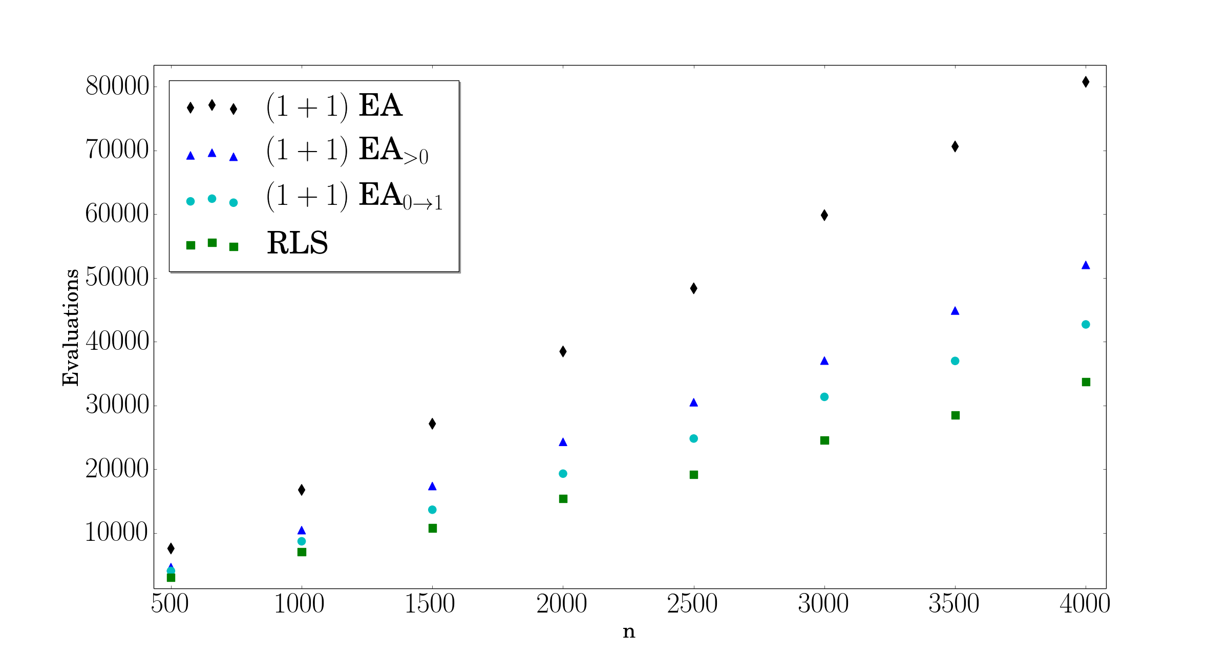
Figure 1: Average runtimes for 100 independent runs of the respective algorithms (with mutation probability $p=1/n$ for the $(1+1)$ EA and its variants) on OneMax for different problem sizes $n$. Statistical data is available in Table LABEL:tab:oeaOM

2.1.2 Performance of the (1+1) EA Variants on Linear Functions

It is well known since the work of Witt [Wit13] that the expected optimization time of the $(1+1)$ EA with mutation probability $p=c/n$ on any linear function $f:\{0,1\}^{n}\rightarrow\mathbb{R},x\mapsto\sum_{i=1}^{n}{w_{i}x_{i}}$ with $w_{1},\ldots,w_{n}\in\mathbb{R}$ equals $(1\pm o(1))\frac{e^{c}}{c}n\ln n$, cf. Theorem 3.1(3) in [Wit13]. With a bit more effort than for the proof of Theorem 5 we can easily generalize Witt’s result to the $(1+1)$ EA_>0. Using the same approach, similar bounds can also be proven for the $(1+1)$ EA_0→1, but we do not do this explicitly in this work.

Theorem 9.

Let $c>0$. The expected optimization time of the $(1+1)$ EA_>0 with mutation probability $p=c/n$ on any linear function $f:\{0,1\}^{n}\rightarrow\mathbb{R},x\mapsto\sum_{i=1}^{n}{w_{i}x_{i}}$ is $(1\pm o(1))\frac{e^{c}-1}{c}n\ln n$.

Proof.

The lower bound follows from Theorem 6 by observing that, just as for the $(1+1)$ EA, also for the $(1+1)$ EA_>0 the easiest to optimize linear function is OneMax [DJW12]; i.e., the expected optimization time of the $(1+1)$ EA_>0 on an arbitrary linear function is at least as large as that on OneMax. In fact, this lower bound holds more generally for any function with unique global optimum.

The upper bound can be easily obtained from the proof of Theorem 4.1 in [Wit13]. One only has to adjust the probabilities of the events in Witt’s proof to account for the fact that the $(1+1)$ EA_>0 samples the number of bits to flip from the conditional binomial distribution $\operatorname{Bin}_{>0}(n,p)$ instead of the unconditional $\operatorname{Bin}(n,p)$ one. This changes the expected drift by a multiplicative factor of $1/(1-(1-p)^{n})$, thus resulting in a multiplicative $(1-(1-p)^{n})$ factor for the runtime estimate. Apart from this small change in the expected drift, the remainder of the proof remains identical. ∎

2.1.3 The (1+1) EA on LeadingOnes.

We now regard LeadingOnes, another classical benchmark problem in the theory of EC. LeadingOnes assigns to each bit string the maximal number of initial ones, i.e., $\textsc{Lo}(x):=\max\{i\in[0..n]\mid\forall j\leq i:x_{j}=1\}$.

Böttcher, B. Doerr, and Neumann showed in [BDN10] that the expected optimization time of the $(1+1)$ EA with mutation probability $p$ on LeadingOnes equals $\frac{1}{2p^{2}}((1-p)^{-n+1}-(1-p))$. This expression is minimized for $p\approx\frac{1.59}{n}$, yielding an expected optimization time of approximately $0.77n^{2}$.

Intuitively, when we ignore iterations with $\ell=0$, the expected optimization time should just decrease by a multiplicative factor of $1-(1-p)^{n}$, just as in the case of OneMax. Building on the proof in [BDN10], it is not difficult to show that this intuition is correct. Interestingly, this observation has been previously made in [JZ11, Theorem 3]. The proof of [BDN10] can also be used to analyze the performance of the $(1+1)$ EA_0→1.

Theorem 10.

The expected optimization time $\mathbb{E}[T_{>0,p}(\textsc{Lo})]$ of the $(1+1)$ EA_>0 with mutation probability $p$ for LeadingOnes equals

$$\frac{1-(1-p)^{n}}{2p^{2}}((1-p)^{-n+1}-(1-p))=\frac{(1-(1-p)^{n})^{2}}{2p^{2}(1-p)^{n-1}},$$

while for the $(1+1)$ EA_0→1 it holds that

$$\mathbb{E}[T_{\operatorname{0\rightarrow 1},p}(\textsc{Lo})]=\frac{1}{2}\sum\limits_{j=0}^{n-1}\frac{1}{p(1-p)^{n-j}+\frac{1}{n}(1-p)^{n}}.$$

The full proof of Theorem 10 for the $(1+1)$ EA_>0 can be found in [JZ11, Section 2], and the one for the $(1+1)$ EA_0→1 is very similar. We nevertheless sketch the main steps and begin by recalling two central theorems from [BDN10]. Böttcher et al. consider an algorithm to be a $(1+1)$ EA-variant if it follows the scheme of Algorithm 1. It is not difficult to see that the following results also apply to the $(1+1)$ EA_>0 and the $(1+1)$ EA_0→1.

Theorem 11 (Theorem 1 in [BDN10]).

Let $x\in\{0,1\}$ be a random point with $\textsc{Lo}(x)<n$. Then for any $(1+1)$ EA-variant $\mathcal{A}$, the time $A_{n-\textsc{Lo}(x)}$ needed to wait to find an improvement satisfies

$$\mathbb{E}[A_{n-\textsc{Lo}(x)}]=\frac{1}{\mathbb{P}[\textsc{Lo}(y)>\textsc{Lo}(x)]},$$

where $y$ denotes the outcome of one iteration of $\mathcal{A}$.

Theorem 12 (Theorem 2 in [BDN10]).

For any any $(1+1)$ EA-variant the expected time needed to find the optimum given a random solution with Lo-value $n-i$ is

$$\mathbb{E}[T_{i}]=\mathbb{E}[A_{i}]+\frac{1}{2}\sum\limits_{j=0}^{i-1}\mathbb{E}[A_{j}],$$

where $A_{j}$ is the time needed to find an improvement starting in a random search point of Lo-value $n-j$.

In this setup, Böttcher et al. show that for the $(1+1)$ EA with mutation probability $p$ it holds that $\mathbb{P}[\textsc{Lo}(y)>\textsc{Lo}(x)]=(1-p)^{j}p$ if $\textsc{Lo}(x)=j$ and conclude that for a fixed mutation rate, the expected optimization time is given by

$$\frac{1}{2p^{2}}((1-p)^{-n+1}-(1-p)).$$

As mentioned above, this expression is minimized for $p\approx 1.59/n$, giving an expected optimization time of $\approx 0.77n^{2}$.

As mentioned above, it is quite intuitive that the probability that the $(1+1)$ EA_>0 leaves fitness level $j$ equals

$$\mathbb{P}[\textsc{Lo}(y)>\textsc{Lo}(x)]=\frac{(1-p)^{j}p}{1-(1-p)^{n}},$$

because all we have to change is to replace the binomial bit flip probabilities by those of the conditional distribution $\operatorname{Bin}_{>0}(n,p)$. This intuitive argument has been formally proven in [JZ11, Theorem 3], resulting in the claimed expected optimization time of the $(1+1)$ EA_>0 of

$$\mathbb{E}[T]=\frac{1-(1-p)^{n}}{2p^{2}}((1-p)^{-n+1}-(1-p))=\frac{(1-(1-p)^{n})^{2}}{2p^{2}(1-p)^{n-1}}.$$ (1)

For the $(1+1)$ EA_0→1 the probability of improvement at a given iteration starting in a random point $x$ with $\textsc{Lo}(x)=j$ is given by

$$\mathbb{P}[\textsc{Lo}(y)>\textsc{Lo}(x)]=p(1-p)^{j}+\frac{1}{n}(1-p)^{n},$$

yielding a total expected optimization time for LeadingOnes of

$$T_{0\to 1} =\frac{1}{2}\sum\limits_{j=0}^{n-1}\frac{1}{p(1-p)^{n-j}+\frac{1}{n}(1-p)^{n}}.$$

For $p=1/n$ the $(1+1)$ EA_>0 thus needs, on average, about $\frac{(e-1)^{2}}{2e}n^{2}\approx 0.543n^{2}$ function evaluations to optimize LeadingOnes. This value is just slightly above the expected optimization time $n^{2}/2$ of RLS. We also see that $\lim_{p\rightarrow 0}{\mathbb{E}[T_{>0,p}(\textsc{Lo})]}=n^{2}/2$. As for OneMax the reason for this is quite simple: the smaller $p$, the more likely we are to sample $\ell=1$, thus resembling an RLS-iteration.

The bound for the $(1+1)$ EA_0→1 is more difficult to interpret, but as in the case of OneMax the convergence to $n^{2}/2$ for $p\to 0$ is faster than that of the $(1+1)$ EA_>0, cf. Table 1, which compares for $n=1\,000$ the expected optimization times of the $(1+1)$ EA, the $(1+1)$ EA_>0, and the $(1+1)$ EA_0→1 for different values of $p$.

$p$	$1/n$	$1/(10n)$	$1/(100n)$
$\mathbb{E}[T_{p}]/n^{2}$	0.8589	5.2583	50.2506
$\mathbb{E}[T_{>0,p}]/n^{2}$	0.5431	0.5004	0.5000
$\mathbb{E}[T_{0\to 1,p}]/n^{2}$	0.5166	0.5000	0.5000

Table 1: Comparison of the expected optimization times of the $(1+1)$ EA, the $(1+1)$ EA_>0, and the $(1+1)$ EA_0→1 with different values of $p$ on LeadingOnes of problem dimension $n=1\,000$. The poor performance of the $(1+1)$ EA stems from the increasing number of iterations in which no bit is flipped at all.

For fixed $p=1/n$ the expected optimization time of the $(1+1)$ EA_0→1 converges to $0.5163n^{2}$. Table 2 compares the expected optimization times of the three algorithms for different values of $n$.

$n$	10	100	1 000	10 000	100 000	1 000 000
$\mathbb{E}[T_{p=1/n}(\textsc{Lo})]/n^{2}$	0.8405	0.8573	0.8589	0.8591	0.8591	0.8591
$\mathbb{E}[T_{>0,p=1/n}(\textsc{Lo})]/n^{2}$	0.5474	0.5435	0.5431	0.5430	0.5430	0.5430
$\mathbb{E}[T_{0\to 1,p=1/n}(\textsc{Lo})]/n^{2}$	0.5536	0.5197	0.5166	0.5163	0.5163	0.5163

Table 2: Comparison of the expected optimization times of the $(1+1)$ EA, the $(1+1)$ EA_>0, and the $(1+1)$ EA_0→1 with $p=1/n$ on LeadingOnes for different problem dimension $n$

Experimental Results. Figure 2 shows for 100 independent runs on LeadingOnes the observed average runtimes of the three different algorithms with mutation rate $p=1/n$ for different problem sizes $n$. While the $(1+1)$ EA_>0 and the $(1+1)$ EA_0→1 have a significantly better performance than the $(1+1)$ EA already for small problem sizes ($38\%$ to $40\%$ for $n=600$), the difference between the two algorithms is much smaller than for OneMax.

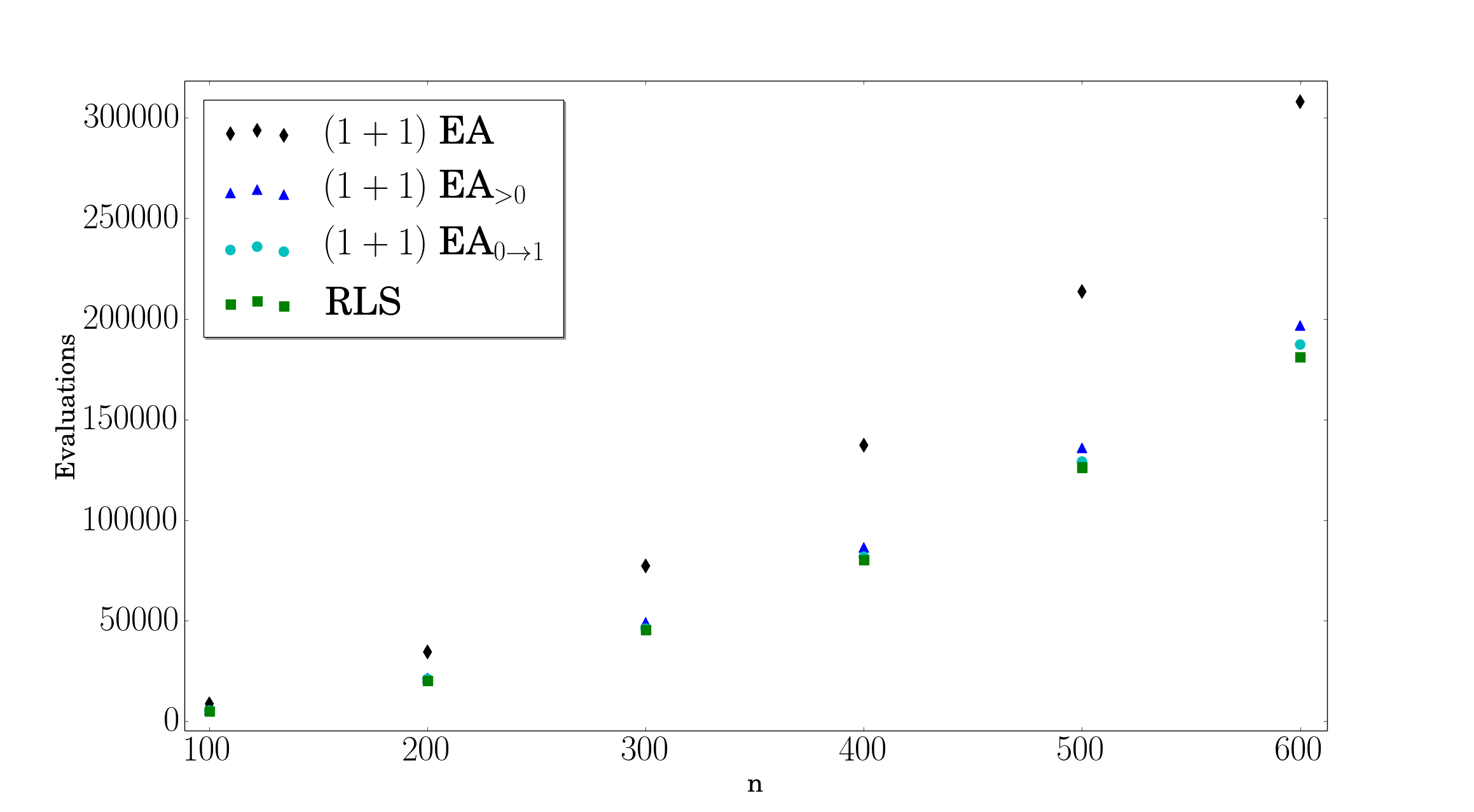
Figure 2: Average runtimes for 100 independent runs of the respective algorithms (with mutation probability $p=1/n$ for the $(1+1)$ EA and its variants) on LeadingOnes for different problem sizes $n$.

2.2 The $(1+(\lambda,\lambda))$ GA and the Greedy $(2+1)$ GA

In the previous section we have made the point that an algorithm should not be charged for iterations in which no bit is flipped. We now discuss that, more generally, one should not count function evaluations in which the sampled offspring equals one of its parents (assuming that this is easy to detect, of course). To this end, we will describe in this section reasonable implementations of the $(1+(\lambda,\lambda))$ GA presented in [DDE15] and the Greedy $(2+1)$ GA from [Sud12]. As mentioned above, we will obtain a quite surprising result, namely that the Greedy $(2+1)$ GA${}_{\text{mod}}$, which we obtain from the Greedy $(2+1)$ GA by ignoring iterations in which the offspring equals one of its two parents, has an expected optimization time on OneMax that is strictly smaller than that of RLS, and, more than that, smaller than that of any other unary unbiased black-box algorithm.

2.2.1 The $(1+(\lambda,\lambda))$ GA

The $(1+(\lambda,\lambda))$ GA is a theory-inspired EA which introduces a novel use of crossover as a repair mechanism to discrete optimization [DDE15]. It keeps in the memory a best so far solution $x$. Every iteration consists of a mutation and a crossover step. In the mutation step, $\lambda$ offspring are created from $x$. To ensure that all these offspring have the same distance from $x$, the mutation strength $\ell$ is sampled from the binomial distribution $\operatorname{Bin}(n,p)$ and all offspring are created by the variation operator $\operatorname{mut}_{\ell}$. In the crossover phase, the best of these offspring $x^{\prime}$ (ties broken uniformly at random) is then recombined, in $\lambda$ independent trials, with $x$, using a biased crossover $\operatorname{cross}_{c}(\cdot,\cdot)$ which, independently for every position $i\in[n]$, chooses the entry from the second argument with probability $c$ and chooses the entry of the first argument otherwise. The best of these $\lambda$ recombined offspring (ties again broken uniformly at random), $y$, replaces $x$ if it is at least as good, i.e., if $f(y)\geq f(x)$.

It was shown in [DD15b, Doe16] that for suitably chosen parameters $\lambda,p,c$ the $(1+(\lambda,\lambda))$ GA has an $\Theta(n\sqrt{\log(n)\log\log\log(n)/\log\log(n)})$ expected runtime on OneMax, thus beating the $\Omega(n\log n)$ bound valid for any mutation-only algorithm [LW12, DDY16b]. The expected performance of the $(1+(\lambda,\lambda))$ GA can be further improved to linear by using non-static parameters, cf. [DDE15, DD15a].

From the above description we see that one iteration of the $(1+(\lambda,\lambda))$ GA costs $2\lambda$ function evaluations, as we have to evaluate the $\lambda$ offspring created in the mutation phase and the $\lambda$ offspring created in the crossover phase. When $\ell=0$, all these $2\lambda$ offspring equal $x$, and thus cause $2\lambda$ useless function evaluations. Our first suggestion is therefore to sample, as in the $(1+1)$ EA_>0, the mutation strength $\ell$ from the conditional binomial distribution $\operatorname{Bin}_{>0}(n,p)$. With the recommended parameter setting $p=\lambda/n$ and $c=1/\lambda$ the probability to sample $\ell=0$ in the unconditional binomial distribution is $(1-p)^{n}=(1-\lambda/n)^{n}\approx\exp(-\lambda)$. Sampling from the conditional distribution thus saves us an expected number of $2\exp(-\lambda)\lambda$ function evaluations per iteration. Our second suggestion concerns the crossover phase. Depending on $\lambda$, whose optimal value approaches $\sqrt{n}$ as fitness increases, the probability $c=1/\lambda$ to take an entry from $x^{\prime}$ can be quite small. It is therefore not unlikely that an offspring created in the crossover phase equals one of its two parents, in particular the original parent $x$. Since this equality can be easily checked, we suggest not to evaluate such offspring. Finally, when the winner $x^{\prime}$ of the mutation phase is better than that of the crossover phase (i.e., if $f(x^{\prime})>f(y)$), we suggest to replace $x$ by $x^{\prime}$ if $f(x^{\prime})\geq f(x)$.

That our suggested changes are indeed practice-driven can be seen by looking at the implementation of the $(1+(\lambda,\lambda))$ GA reported in [GP15], which is available on GitHub [Gol]. Indeed, all of the suggested changes have been implemented there. Our $(1+(\lambda,\lambda))$ GA${}_{\text{mod}}$ ignores, however, some additional problem-driven changes made in [GP15].

For the $(1+(\lambda,\lambda))$ GA on OneMax only asymptotic runtime bounds are available [DD15b, Doe16, DDE15]. We can therefore at the moment not compute the optimal parameter values of the $(1+(\lambda,\lambda))$ GA${}_{\text{mod}}$. For our experiments we use the self-adjusting choice of $\lambda$ proposed and analyzed in [DD15a], both for the $(1+(\lambda,\lambda))$ GA as well as for the $(1+(\lambda,\lambda))$ GA${}_{\text{mod}}$. This self-adjusting choice yields linear expected runtime on OneMax and works as follows. In the beginning, $\lambda$ is initialized as $\lambda=1$. At the end of each iteration, it is checked if the iteration was successful. If so, i.e., if $f(y)>f(x)$, then $\lambda$ is decreased to $\lambda/F$, and it is increased to $\lambda\cdot F^{1/4}$ otherwise. For our experiments we use $F=1.5$. With this self-adjusting rule the $(1+(\lambda,\lambda))$ GA${}_{\text{mod}}$ becomes Algorithm 13.

1Initialization: Choose $x\in\{0,1\}^{n}$ u.a.r. and evaluate $f(x)$;

2 Initialize $\lambda\leftarrow 1$;

3 Optimization: for $t=1,2,3,\ldots$ do

4       Mutation phase:

5       Sample $\ell$ from $\operatorname{Bin}_{>0}(n,p)$;

6       for $i\in[\lambda]$ do $x^{(i)}\leftarrow\operatorname{mut}_{\ell}(x)$; Evaluate $f(x^{(i)})$;

7       Choose $x^{\prime}\in\{x^{(i)}\mid i\in[\lambda]\}$ with $f(x^{\prime})=\max\{f(x^{(i)})\mid i\in[\lambda]\}$ u.a.r.;

8       Crossover phase:

9       for $i\in[\lambda]$ do $y^{(i)}\leftarrow\operatorname{cross}_{c}(x,x^{\prime})$; if $y^{(i)}\notin\{x,x^{\prime}\}$ then evaluate $f(y^{(i)})$;

10       Choose $y\in\{y^{(i)}\mid i\in[\lambda]\}\cup\{x^{\prime}\}$ with $f(y)=\max\left(\{f(y^{(i)})\mid i\in[\lambda]\}\cup\{f(x^{\prime})\}\right)$ u.a.r.;

11       Selection and update step:

12       if $f(y)>f(x)$ then  $x\leftarrow y$; $\lambda\leftarrow\max\{\lambda/F,1\}$;

13       if $f(y)=f(x)$ then  $x\leftarrow y$; $\lambda\leftarrow\min\{\lambda F^{1/4},n\}$;

14       if $f(y)<f(x)$ then $\lambda\leftarrow\min\{\lambda F^{1/4},n\}$;

15      

Algorithm 13 (The self-adjusting $(1+(\lambda,\lambda))$ GA${}_{\text{mod}}$, maximizing $f:\{0,1\}^{n}\to\mathbb{R}$, with offspring population size $\lambda$, mutation probability $p$, crossover bias $c$, and update strength $F$. ).

2.2.2 The Greedy $(2+1)$ GA

As in [DDE15], we compare the $(1+(\lambda,\lambda))$ GA and the $(1+(\lambda,\lambda))$ GA${}_{\text{mod}}$ with the Greedy $(2+1)$ GA from Sudholt [Sud12]. The Greedy $(2+1)$ GA, or more generally, the greedy $(\mu+1)$ GA presented in [Sud12] maintains a population $\mathcal{P}$ of $\mu$ individuals. $\mathcal{P}$ is initialized by sampling $\mu$ search points independently and uniformly at random. Each iteration consists of two steps, a crossover step and a mutation step. In the crossover step two parents $x,y$ are selected uniformly at random (with replacement) from those individuals $u\in\mathcal{P}$ for which $f(u)=\max_{v\in\mathcal{P}}{f(v)}$ holds. Note that if there is only one such search point, then this one is selected twice. From these two search points an offspring $z^{\prime}$ is created by uniform crossover $\operatorname{cross}_{1/2}(x,y)$. This offspring $z^{\prime}$ is then mutated by standard bit mutation, i.e., each bit is flipped independently with some probability $p\in[0,1]$. The so-created offspring $z$ is evaluated. If $z\notin\mathcal{P}$ and its fitness is at least as good as $\min_{v\in\mathcal{P}}f(v)$, it replaces the worst individual in the population, ties broken uniformly at random. The requirement $z\notin\mathcal{P}$ is a so-called diversity mechanism.

It is not difficult to see that from the whole population only those with a best-so-far fitness value are relevant, the others are never selected for reproduction. Furthermore we see that in the case that $\mu=2$, even if there are two different individuals $x\neq y$ in the population $\mathcal{P}$, the probability to select both of them for reproduction is only $1/2$. In all other cases the crossover phase just reproduces one of the two parents. We change this in our implementation and enforce that in the crossover phase both parents are selected if they have an equal fitness value. As we shall discuss below, this change does not influence our upper bounds much (it changes the constant in the linear term of the overall $\Theta(n\ln n)$ expected runtime, but does not affect the leading constant of the $n\ln(n)$ term), but we believe that in particular for $\mu=2$ this variant is more “natural”. Sudholt showed for his Greedy $(2+1)$ GA that its expected optimization time on OneMax is at most

$$\frac{\ln(n^{2}p+n)+1+p}{p(1-p)^{n-1}(1+np)}+\frac{8n}{(1-p)^{n}}.$$

It is very easy to modify his proof to show that the expected optimization time of the Greedy $(2+1)$ GA with the new parental selection is at most

$$\frac{\ln(n^{2}p+n)+1+p}{p(1-p)^{n-1}(1+np)}+\frac{4n}{(1-p)^{n}},$$

i.e., an additive term of $\frac{4n}{(1-p)^{n}}$ smaller than the original Greedy $(2+1)$ GA.

We now modify the Greedy $(2+1)$ GA in a similar way as we did for the $(1+(\lambda,\lambda))$ GA, cf. Algorithm 14. Our first modification is that we do not evaluate $z$ if it equals one of its parents $x$ or $y$. Our second modification concerns the mutation phase. When $z^{\prime}\in\{x,y\}$, we enforce a mutation strength greater than $0$ by sampling from the conditional distribution $\operatorname{Bin}_{>0}(n,p)$. Note that $z^{\prime}\in\{x,y\}$ holds when the crossover did not happen (i.e., if $f(x)>f(y)$ in line 14 of Algorithm 14) or when the random choices of the crossover resulted in a string that equals one of its two parents. If we denote by $d$ the Hamming distance of $x$ and $y$ this latter event happens with probability $1/2^{d-1}$. The situation $d=H(x,y)=2$ occurs quite frequently, resulting in a $1/2$ probability that the crossover reproduces one of the two parents.

1Choose $x$ and $y$ from $\{0,1\}^{n}$ independently and u.a.r. and evaluate $f(x),f(y)$;

2 for $t=1,2,3,\ldots$ do

3       Ensure $f(x)\geq f(y)$ by renaming them if needed;

4       if $f(x)=f(y)$ then $z^{\prime}\leftarrow\operatorname{cross}_{1/2}(x,y)$; else $z^{\prime}\leftarrow x$;

5       if $z^{\prime}\notin\{x,y\}$ then Sample $\ell$ from $\operatorname{Bin}(n,p)$; else Sample $\ell$ from $\operatorname{Bin}_{>0}(n,p)$;

6       $z\leftarrow\operatorname{mut}_{\ell}(z^{\prime})$;

7       if $z\notin\{x,y\}$ then

8             evaluate $f(z)$;

9             if $f(z)\geq f(y)$ and $f(y)<f(x)$ then $y\leftarrow z$;

10             if $f(z)\geq f(y)=f(x)$ then replace either $y$ or $x$ by $z$, chosen u.a.r.;

11            

12      

Algorithm 14 (The Greedy $(2+1)$ GA${}_{\text{mod}}$ with mutation probability $p$ maximizing a given function $f:\{0,1\}^{n}\to\mathbb{R}$).

Following very closely the proof of Theorem 2 in [Sud13], it is not difficult to obtain the following runtime statement.

Theorem 15.

The expected optimization time of the Greedy $(2+1)$ GA${}_{\text{mod}}$ with mutation rate $p$ is at most $\frac{(1-(1-p)^{n})(\ln(n^{2}p+n)+1+p)}{p(1-p)^{n-1}(1+np)}+\frac{4n}{(1-p)^{n}}.$ For $p=c/n$ the expected optimization time is thus at most

$$\frac{(1-(1-c/n)^{n})}{c(1-c/n)^{n-1}(1+c)}n\ln(n)+\Theta(n).$$ (2)

Proof.

Following [Sud12], we say that the algorithm is on fitness level $i$ if the best individual in the population has fitness value $i$. Like Sudholt, we distinguish two cases.

Case $i$.1: $i=f(x)$ and either $f(x)>f(y)$ or $x=y$. In this situation there is no crossover. The offspring $z$ is the outcome of standard bit mutation on $x$. The algorithm leaves this situation when (a) $f(z)>i$ or (b) $f(z)=f(x)$ and $z\neq x$. The probability for (a) to happen is at least $(n-i)p(1-p)^{n-1}/(1-(1-p)^{n})$, since this is the probability that exactly one of the zero bits is flipped in the mutation phase. Likewise, the probability of event (b) is $i(n-i)p^{2}(1-p)^{n-2}/(1-(1-p)^{n})$. Once the algorithm has left case i.1 it does never return to it. This is ensured by the diversity mechanism, which allows to include $z$ in the population only if it isn’t yet (line 14 of Algorithm 14). The total expected time spent in the cases $i$.1, $i=0,\ldots,n-1$ is therefore at most

$$\frac{1-(1-p)^{n}}{p(1-p)^{n-1}}\sum_{i=0}^{n-1}{\frac{1}{(n-i)(1+ip)}}.$$

The same algebraic computations as in [Sud12] show that this expression can be bounded from above by

$$\frac{(1-(1-p)^{n})(\ln(pn^{2}+n)+1+p)}{p(1-p)^{n-1}(1+np)}.$$

Case $i$.2: $i=f(x)=f(y)$ and $x\neq y$. In this case the Hamming distance of $x$ and $y$ is even. Let $X$ denote the number of ones in the intermediate offspring $z^{\prime}$ in those $2d$ positions in which $x$ and $y$ differ. $X$ is binomially distributed with $2d$ trials and success probability $1/2$. It is not difficult to show that $\mathbb{P}[X>d]\geq 1/4$. When $X>d$, then $z^{\prime}\notin\{x,y\}$ and the mutation strength is therefore sampled from the binomial distribution $\operatorname{Bin}(n,p)$. The probability to sample a zero is $(1-p)^{n}$. Thus, the probability to leave fitness level $i$ is at least $(1-p)^{n}/4$ and the total expected time spent in the cases $i$.2, $i=0,\ldots,n-1$ is at most $4n/(1-p)^{n}$. ∎

For large $n$, we can approximate expression (2) by $\frac{(1-\exp(-c))}{c\exp(-c)(1+c)}n\ln(n)+\Theta(n)$, which is minimized for $c\approx 0.773581$, yielding an expected optimization time of approximately $(1+o(1))0.850953n\ln(n)$ for the Greedy $(2+1)$ GA${}_{\text{mod}}$, cf. Table 3 for the values of $c$ minimizing $\frac{1-(1-c/n)^{n}}{c(1-c/n)^{n-1}(1+c)}$ for different values of $n$. For comparison, the expected optimization time of RLS is $(1\pm o(1))n\ln(n)$, and so is the expected optimization time of the best possible unary unbiased black-box algorithm [DDY16b]. This is a quite remarkable result, as it seems to be the first time that a “classic” GA is shown to outperform RLS on OneMax.

$n$	10	100	500	$1\,000$	$5\,000$
$c$	0.783953	0.774577	0.773778	0.773679	0.773599
$\frac{1-(1-c/n)^{n}}{c(1-c/n)^{n-1}(1+c)}$	0.831839	0.859091	0.850581	0.850766	0.850915

Table 3: Values of $c$ minimizing expression (2) for different values of $n$

It is beyond the scope of this work to analyze the tightness of the upper bounds proven in Theorem 15, and additional gains may be possible by choosing different values for $p$. Our empirical results suggest that the upper bound of Theorem 15 is indeed rather weak. We also remark that RLS${}_{\text{opt}}$ (described below), the RLS-variant from [DDY16b] achieving the (up to lower order term) optimal run time among all unary unbiased black-box algorithms on OneMax, uses fitness-dependent mutation rates. It is possible (and likely) that the Greedy $(2+1)$ GA${}_{\text{mod}}$, as well, could profit further from choosing the mutation rate in such an adaptive way. We have to leave this for future work.

RLS${}_{\text{opt}}$ is essentially RLS, with the only difference that in the mutation step, instead of flipping always one random bit, more than one bit can be flipped. Intuitively, the optimal number $\ell^{*}_{v}$ of bits to flip depends only on the fitness value $v=\textsc{Om}(x)$ of the current-best individual $x$ and should be the one that maximizes the expected progress $\mathbb{E}[\max\{\textsc{Om}(y)-\textsc{Om}(x),0\}\mid\textsc{Om}(x)=v,y=\operatorname{mut}_{\ell}(x)]$. That this drift maximizer is indeed (at least up to the mentioned additive $O(n)$ term) optimal has been formally proven in [DDY16b]. More precisely, it is shown that the expected runtime of RLS${}_{\text{opt}}$ on OneMax and the unary unbiased black-box complexity of OneMax both are $n\ln(n)-cn\pm o(n)$ for a constant $c$ between 0.2539 and 0.2665. To run RLS${}_{\text{opt}}$ in our experiments, we have computed, for every tested $n$ and every fitness value $v\in[0..n-1]$ the value $\ell^{*}_{v}$ that maximizes the expected drift

$$B(n,v,\ell) :=\mathbb{E}[\max\{\textsc{Om}(y)-\textsc{Om}(x),0\}\mid\textsc{Om}(x)=v,y=\operatorname{mut}_{\ell}(x)]$$

$$=\sum_{i=\lceil\ell/2\rceil}^{\ell}\frac{\binom{n-v}{i}\binom{v}{\ell-i}\left(2i-\ell\right)}{\binom{n}{\ell}},$$ (3)

i.e., we do not work with the approximation proposed in [DDY16b] but the original drift maximizer.

2.2.3 Experimental Results

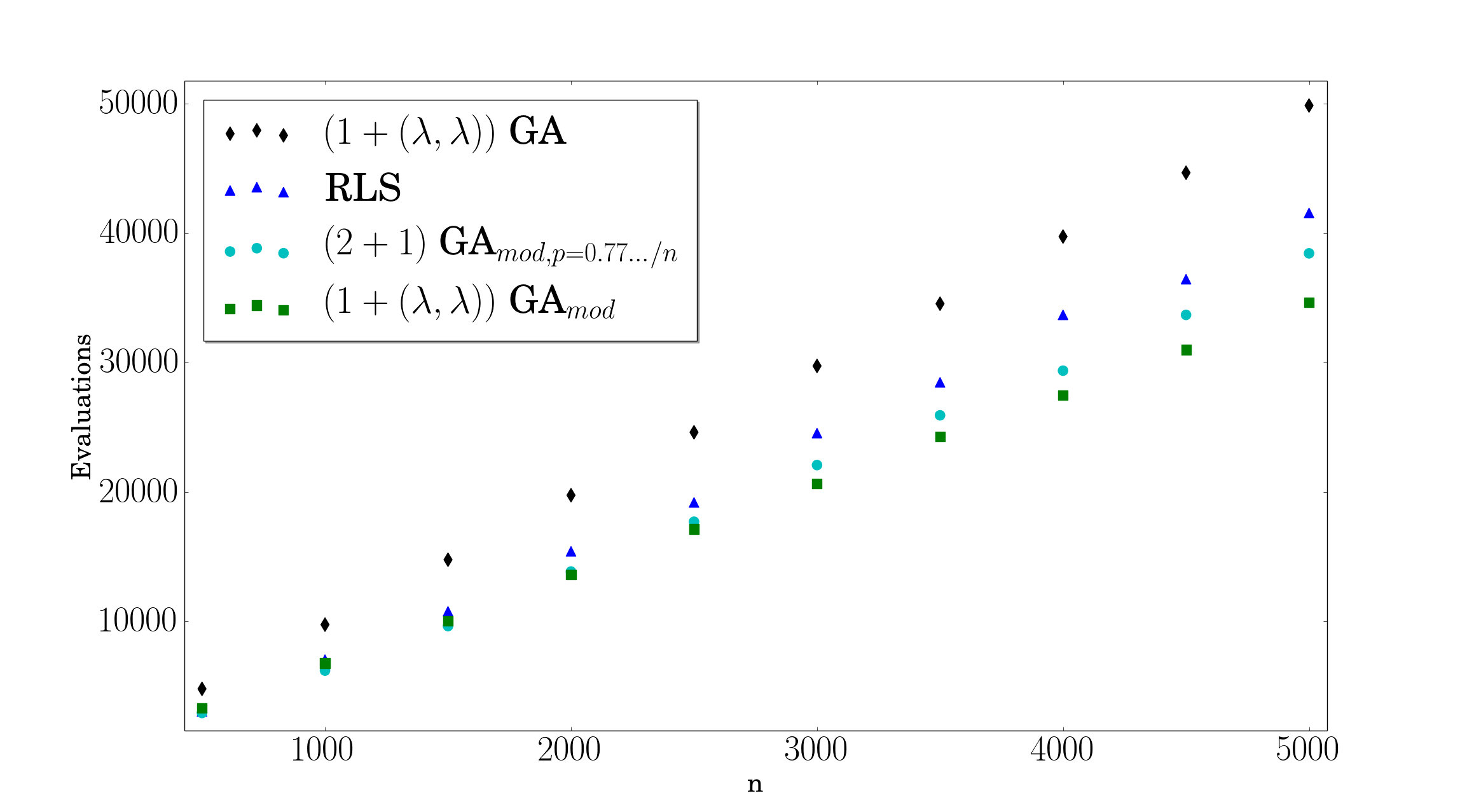
Figure 3: Average runtimes for 100 independent runs of the respective algorithms on OneMax for different problem sizes $n$.

Figure 3 shows experimental data for the performance of the mentioned algorithms on OneMax, for $n$ ranging from $100$ to $5\,000$. The $(1+(\lambda,\lambda))$ GA and the $(1+(\lambda,\lambda))$ GA${}_{\text{mod}}$ use the self-adjusting $\lambda$ values, while for the Greedy $(2+1)$ GA${}_{\text{mod}}$ we use mutation rate $0.773581/n$. In the reported ranges, the expected performance of the Greedy $(2+1)$ GA with mutation rate $p=(1+\sqrt{5})/(2n)$ is very similar to that of the self-adjusting $(1+(\lambda,\lambda))$ GA (cf. Figure 8 in [DDE15]); we do not plot these data points to avoid an overloaded plot. Detailed statistical information for these data points is given in Table LABEL:tab:ga. We observe that both the $(1+(\lambda,\lambda))$ GA${}_{\text{mod}}$ as well as the Greedy $(2+1)$ GA${}_{\text{mod}}$ are better than RLS already for quite small problem sizes. We also observe that, in line with the theoretical bounds, the advantage of the $(1+(\lambda,\lambda))$ GA${}_{\text{mod}}$ over the Greedy $(2+1)$ GA${}_{\text{mod}}$ and over RLS increases with the problem size.

3 Runtime Profiles

Most runtime results in discrete EC are statements about first hitting times, understood as the time needed by an algorithm until it evaluates for the first time an optimal solution of the underlying problem. In particular the expected value of this random variable is studied. However, in almost all practical applications, the user does not know when the algorithm is “done”. And even if this could be detected, it may take too long for this event to happen. It is therefore highly relevant to understand how the algorithms perform over time. Jansen and Zarges [JZ14], for this reason, suggested to adopt a fixed-budget perspective, analyzing the expected fitness value that an algorithm has achieved after a fixed number of iterations. Here in this work we suggest a complementary view.

Instead of reporting only the expected time needed to hit, for the first time, an optimal solution, we suggest to include in the runtime statements the expected time needed to hit intermediate fitness values. When canonical fitness levels exits, such as in the case of OneMax, LeadingOnes, royal road, and several other functions, we suggest to use these. For other functions, such as linear functions or weighted combinatorial graph problems, the analysis of the expected optimization time often identifies useful to report target fitness levels. In the absence of these, a linear interpolation of the minimal and maximal fitness value could be used. We call such statements runtime profiles. We emphasize the fact that runtime profiles have, very naturally, been reported in many empirical works on heuristic optimization. We are thus not suggesting any new concept here. Our intention is rather to highlight to researchers working on theoretical aspects in evolutionary computation that, beyond being possibly more relevant for practitioners, explicitly reporting runtime profiles can give quite interesting insights into the performance of EAs.

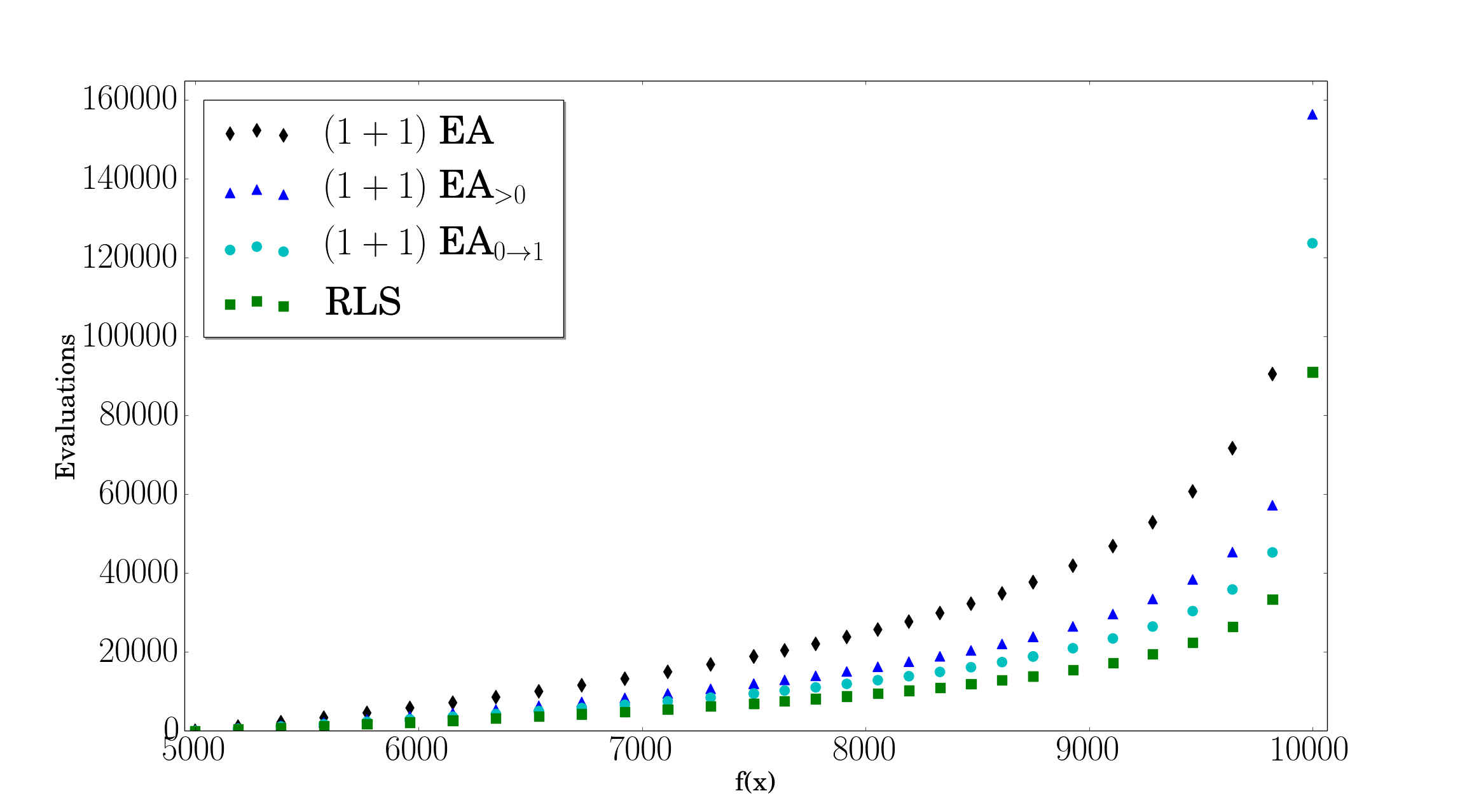
Figure 4: Runtime profiles on OneMax for problem size $n=10\,000$ according to the bounds computed in Theorem 16 but assuming to start in a search point of fitness value $n/2$.

Note that, in contrast to the previous section, our suggestion does not change any of the algorithms nor the runtime bounds. We merely suggest to report them in a different way. All bounds reported below can be easily obtained from previous works and are more or less explicit in previous proofs.

Theorem 16.

Let $p\in(0,1)$ and $k\in[n]$. Starting in the all-zeros string $x=(0,\ldots,0)$ the expected time needed to reach for the first time a search point $x$ of OneMax-value at least $k$ is at most

• $n(H_{n}-H_{n-k})$ for RLS,

• $\frac{1}{p(1-p)^{n-1}}(H_{n}-H_{n-k})$ for the $(1+1)$ EA with mutation probability $p$,

• $\frac{1-(1-p)^{n}}{p(1-p)^{n-1}}(H_{n}-H_{n-k})$ for the $(1+1)$ EA_>0 with mutation probability $p$, and

• $\frac{1}{(1-p)^{n-1}(p+1/n-p/n)}(H_{n}-H_{n-k})$ for the $(1+1)$ EA_0→1 with mutation probability $p$.

For $p=1/n$ these bounds are $(1\pm o(1))Cn(H_{n}-H_{n-k})$, where $C=e$ for the $(1+1)$ EA, $C=e-1$ for the $(1+1)$ EA_>0, and $C=e/(2-\frac{1}{n})$ for the $(1+1)$ EA_0→1.

Note that the theorem bounds the time needed to reach fitness level $k$ when starting in a search point of fitness 0. This is a very pessimistic view. In a typical run of these algorithms, already the first search point has an expected fitness of roughly $n/2$ and the probability that it is less than $\frac{n}{2}-\sqrt{n}$ is $o(1)$. In consequence, the empirically observed time needed to reach fitness value $k>n/2$ equals roughly the above-stated bounds minus the time needed to reach fitness level $n/2$, cf. also [DD16] where it is formally proven that for RLS the total expected optimization time is almost identical to that deterministically starting in a search point of fitness $n/2$. In Figure 4 we plots the computed runtime profiles for $n=10\,000$, where we assume to start in a search point of fitness $n/2$, i.e., we subtract from the bounds in Theorem 16 the time needed to reach fitness level $n/2$. We see that the performance of the $(1+1)$ EA_>0, the $(1+1)$ EA_0→1 and RLS are quite close for most of the intermediate levels, much closer than what the total optimization time might suggest.

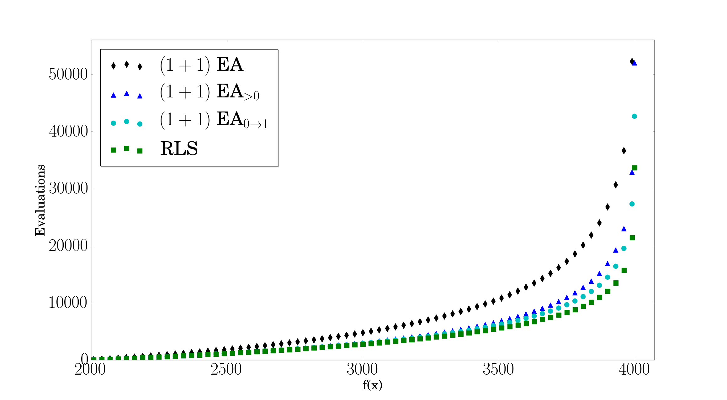
Figure 5: Runtime profile for 100 independent runs of the respective algorithms on OneMax for problem size $n=4\,000$.

In Figure 5 we plot the empirical runtime profiles for 100 independent runs of the different algorithms (with mutation rate $p=1/n$ for the $(1+1)$ EA-variants) on OneMax with $n=4\,000$. The behavior is much similar to our predicted one from Figure 4. In particular, we observe that for all target values $i$, the $(1+1)$ EA needs longest, on average, to reach this fitness level. We also easily see from this plot that all four algorithms easily make progress in the beginning. The waiting time for fitness improvement increases with increasing fitness values. While the expected optimization times of RLS, the $(1+1)$ EA_>0 with mutation rate $p=1/n$, and the $(1+1)$ EA_0→1 with the same mutation rate differs significantly for $n=4\,000$, the expected time to reach the intermediate fitness values is not that diverse for all but the last $10\%$ of the target fitness values.

While for OneMax RLS seems to be consistently better for all relevant intermediate fitness levels, the situation for LeadingOnes is quite different.

Theorem 17.

Let $p\in(0,1)$ and $k\in[n]$. The expected time needed to reach for the first time a search point $x$ of LeadingOnes-value at least $k$ is at most

• $kn/2$ for RLS,

• $\frac{1}{2p^{2}}((1-p)^{1-k}-(1-p))$ for the $(1+1)$ EA with mutation probability $p$,

• $\frac{1-(1-p)^{n}}{2p^{2}}((1-p)^{1-k}-(1-p))$ for the $(1+1)$ EA_>0 with mutation probability $p$,

• $\frac{1}{2}\sum\limits_{i=n-k+1}^{n}\frac{1}{p(1-p)^{n-i}+\frac{1}{n}(1-p)^{n}}$ for the $(1+1)$ EA_0→1 with mutation probability $p$.

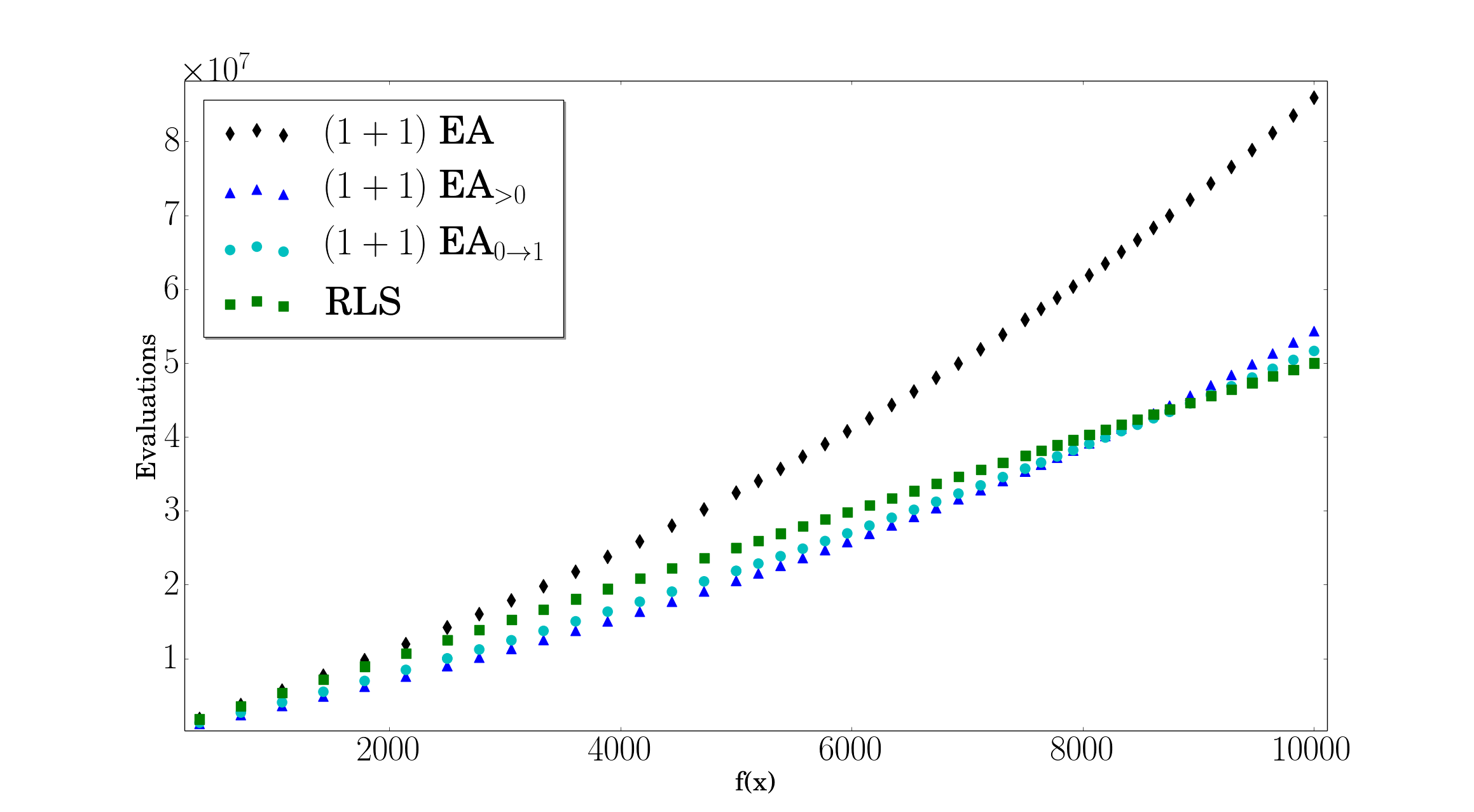
Figure 6: Runtime profile of the respective algorithms (with mutation rate $p=1/n$ for the $(1+1)$ EA and its variants) on LeadingOnes for problem size $n=10\,000$ according to Theorem 17.

As above we plot these computed runtime profiles in Figure 6. We observe that the $(1+1)$ EA_>0 is the best of all four algorithms for intermediate fitness levels $\leq 7\,980$. The $(1+1)$ EA_0→1 has the smallest expected runtime to reach the intermediate fitness values between $7\,980$ to $8\,998$, while RLS is the best of the four algorithms only for fitness levels $i>8\,999$. RLS is faster than the $(1+1)$ EA_>0 for intermediate fitness values $i>8\,566$. As mentioned above, such insights are very important for the design of parameter/operator selection schemes.

In Figure 7 we show the empirically observed runtime profiles for 100 independent runs of the different algorithms on LeadingOnes with $n=500$. We observe that, as our theoretical bounds suggest, the $(1+1)$ EA_>0 ($(1+1)$ EA_0→1) needs less iterations in expectation than RLS to reach fitness values $i\leq 430$ ($i\leq 460$), while RLS, on average, reaches fitness levels $i>430$ ($i>460$) faster. The theoretical bounds in Theorem 17 suggest cut-off points at $i=429$ ($i=449$), matching our empirical findings quite well. Statistical information for this experiment can be found Table LABEL:tab:LOprofile.

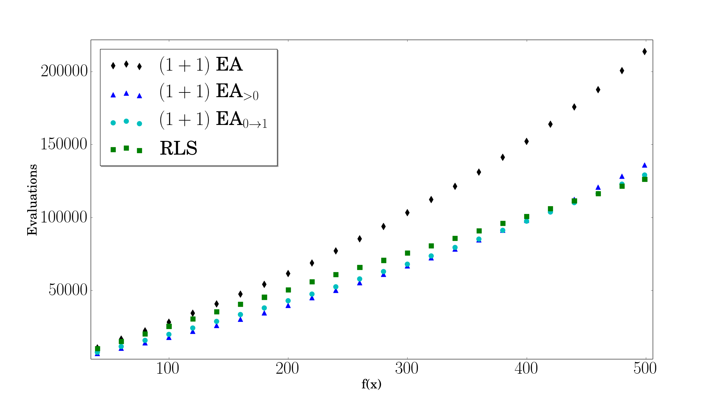
Figure 7: Runtime profile for 100 runs of the respective algorithms (with mutation rate $p=1/n$ for the $(1+1)$ EA and its variants) on LeadingOnes for problem size $n=500$.

4 Discussion and Future Works

We hope to trigger with this work an extended discussion on how to make theoretical results in the domain of evolutionary computation more relevant and interpretable for practitioners. We have suggested two different steps into this direction, (1) do not charge an algorithm for function evaluations when the offspring equals one of its parents (in case this is easy to detect), and (2) report first hitting times not only for the optimum but also for intermediate fitness levels. Naturally, our work can only be a pointer to a more practice-aware theory, and we are aware that there are many more steps that have to be taken. In particular, we believe that the following observations need to be discussed in more detail.

• Many runtime statements report only expected optimization times. However, it is often interesting to understand the probability distribution of the optimization time, in particular for problems where the variance can be large. Runtime analysis has recently seen an increased interest in these runtime distributions, cf., for example, [DG13, Köt16] and follow-up works.

• Similar to the previous point, problems exist where the expected optimization time can be very large even if the probability to hit an optimal solution within a small number of iterations is small. In [DL15] a so-called $p$-Monte Carlo complexity measure has been introduced, measuring the expected time to hit an optimal solution with probability at least $1-p$. Similar suggestions can be found in [ZLLH12].

• The runtime profiles suggested in Section 3 complements the fixed-budget view advocated by Jansen and Zarges [JZ14]. We feel that there is a need for combined measures that are capable of describing the anytime behavior of an EA. Regret-based measure as used in machine learning could be a key here, but we haven’t been able so far to identify a fully satisfying measure.

From a theoretical point of view, our suggested changes are easily implementable. Our work has nevertheless unveiled a quite remarkable result, the superiority of the Greedy $(2+1)$ GA${}_{\text{mod}}$ over any unary unbiased black-box algorithm. We are confident that our performance measure will yield similar results for other problems and algorithms, with the potential of changing our view on fundamental questions like the benefits of crossover over mutation, (dis-)advantages of elitism vs. non-elitism, etc.

Acknowledgments.

We would like to thank Benjamin Doerr, Nikolaus Hansen, and Olivier Teytaud for several independent discussions around the topics of this work.

Our research benefited from the support of the “FMJH Program Gaspard Monge in optimization and operation research”, and from the support to this program from EDF.

Parts of our work have been inspired by COST Action CA15140: Improving Applicability of Nature-Inspired Optimisation by Joining Theory and Practice (ImAppNIO).

Appendix A A Comment on the Benchmark Functions

Theoretical works are often criticized for regarding highly artificial benchmark problems. Indeed, while the power of EAs is certainly to be seen in applications to highly complex problems not admitting a thorough theoretical analysis, theoreticians regard simple benchmark functions like OneMax and LeadingOnes in the hope that, among other reasons,

• they give insights into how the studied algorithms perform on the easier parts of a difficult optimization problem,

• in order to understand some basic working principles of the algorithms, which can then be used for the analysis of more complex problems, more complex algorithms, for the development of new algorithmic ideas, etc.,

• the theoretical investigations, which even for seemingly simple algorithms and problems can be surprisingly complex, triggers the development of new analytical tools for the analysis of randomized algorithms, and

• for very precise mathematical statements a comparison between theoretical results and empirical performance can be made, helping us understand, for example, how the parameter choice influences the optimization time (and how the suggestions obtained via a thorough mathematical analysis differs from that obtained by empirical means).

We furthermore note that even for OneMax and LeadingOnes, despite being studied since the very early days of theory of evolutionary computation, several unsolved problems exist, many of which are of seemingly simple nature such as the optimal dynamic mutation rate of the $(1+1)$ EA for OneMax. Several important advances could be made in the last few years. These results have often required the development of rather sophisticated mathematical tools, as is witnessed by the different drift analysis theorems that have been developed in the last 7 years.

While we are certainly aware that the insights obtained from these benchmark problems (and the simplified evolutionary algorithms) may not always or not easily transfer to more realistic real-world optimization challenges, the concepts proposed in this work are applicable to a very broad range of theory- as well as practice-driven algorithms and problems.

A.1 Unbiasedness

We would also like to point out that all the algorithms considered in this work are unbiased in the sense of Lehre and Witt [LW12], i.e., their runtimes are identical for all functions that are obtained from the considered benchmark problems by composing them with a Hamming-distance preserving automorphism of the hypercube. We recall that a Hamming-automorphism of the hypercube is a one-to-one mapping $\sigma:\{0,1\}^{n}\rightarrow\{0,1\}^{n}$ such that for all $x,y\in\{0,1\}^{n}$ it holds that the Hamming distance $H(x,y)$ equals that of the images $H(\sigma(x),\sigma(y))$. The composition $f\circ\sigma$ of a pseudo-Boolean function $f:\{0,1\}^{n}\rightarrow\mathbb{R}$ with a Hamming-automorphism $\sigma$ has a fitness landscape that is isomorphic to that of $f$ .

For OneMax this implies that all algorithms considered in this work behave identically on all functions of the form $\textsc{Om}_{z}:\{0,1\}^{n}\rightarrow\mathbb{R},x\mapsto|\{i\in[n]\mid x_{i}=z_{i}\}|$, where $z$ is an arbitrarily chosen binary string of length $n$. That is, all results reported for OneMax apply to any of these generalized functions $\textsc{Om}_{z}$.

Similarly, for LeadingOnes, the composed functions are those of the form $\textsc{Lo}_{z,\pi}(x):=\max\{i\in[0..n]\mid\forall j\leq i:z_{\pi(j)}=x_{\pi(j)}\}$, where $\pi$ is an arbitrary permutation of $[n]$ and $z$ an arbitrary binary string of length $n$. All results stated in this report for Lo applies to any of these generalized functions $\textsc{Lo}_{z,\pi}$.

Appendix B Tables with Statistical Data for the Experimental Results

B.1 Statistical Details for Figure 1

		Percentile						StdDev/
$n$	Algorithm	2	25	50	75	98	Mean	Mean
500	$(1+1)$ EA	4885	6468	7436	8538	11566	7569	22.3%
500	$(1+1)$ EA>0	3039	3919	4370	5125	7245	4642	21.8%
500	$(1+1)$ EA0→1	2617	3430	3986	4443	5790	4045	19.9%
500	RLS	2029	2493	2837	3491	4549	3050	23.4%
1000	$(1+1)$ EA	11803	14508	16137	17882	26448	16755	20.4%
1000	$(1+1)$ EA>0	6855	9055	10067	11556	16313	10445	21.6%
1000	$(1+1)$ EA0→1	6402	7416	8435	9459	13246	8697	18.8%
1000	RLS	4922	6024	6887	7660	10031	7046	20.5%
1500	$(1+1)$ EA	20044	23308	26176	28633	43838	27129	20.5%
1500	$(1+1)$ EA>0	11686	14839	16722	19588	26537	17358	19.3%
1500	$(1+1)$ EA0→1	9412	11823	12998	14745	21422	13647	20.2%
1500	RLS	7761	9761	10618	11662	14660	10781	15.4%
2000	$(1+1)$ EA	25377	32941	36046	42765	58925	38462	20.7%
2000	$(1+1)$ EA>0	16741	21482	24132	25998	36370	24290	17.8%
2000	$(1+1)$ EA0→1	13901	17286	19091	20668	26092	19302	15.5%
2000	RLS	10721	13095	14798	17374	21276	15412	20.3%
2500	$(1+1)$ EA	34627	41715	47842	52869	67674	48362	16.6%
2500	$(1+1)$ EA>0	21738	27207	29369	33089	41874	30495	17.2%
2500	$(1+1)$ EA0→1	18977	22062	23831	27042	33713	24809	14.8%
2500	RLS	14113	17054	18776	20921	26823	19192	15.2%
3000	$(1+1)$ EA	45746	51345	58094	65037	83549	59835	16.6%
3000	$(1+1)$ EA>0	29319	32940	36178	39756	48863	37028	14.7%
3000	$(1+1)$ EA0→1	22933	27044	30269	33849	47995	31344	18.9%
3000	RLS	17045	21361	23586	26998	36154	24547	17.9%
3500	$(1+1)$ EA	53926	62548	68329	76639	97308	70608	15.6%
3500	$(1+1)$ EA>0	32088	38664	42530	47916	63506	44874	18.4%
3500	$(1+1)$ EA0→1	24333	33279	36474	39726	50482	36979	15.6%
3500	RLS	22385	25164	27867	31124	38292	28471	14.3%
4000	$(1+1)$ EA	60303	73419	78445	87109	106910	80743	13.6%
4000	$(1+1)$ EA>0	38121	46779	50841	56137	68302	52036	15.1%
4000	$(1+1)$ EA0→1	32561	37462	41529	46539	59900	42703	16.1%
4000	RLS	24922	29349	33493	36808	48134	33684	17.4%

B.2 Statistical Details for Figure 2

		Percentile						StdDev/
$n$	Algorithm	2	25	50	75	98	Mean	Mean
100	$(1+1)$ EA	5431	7789	8637	9460	11877	8580	17.2%
100	$(1+1)$ EA>0	3761	4831	5465	6104	8069	5574	18.5%
100	$(1+1)$ EA0→1	3380	4434	5072	5615	7787	5194	19.1%
100	RLS	3017	4391	4955	5565	6598	5005	16.9%
200	$(1+1)$ EA	25751	31088	34581	37314	41683	34400	12.1%
200	$(1+1)$ EA>0	15687	19686	21026	23129	27120	21438	12.5%
200	$(1+1)$ EA0→1	15589	18985	21164	22697	26539	20970	12.9%
200	RLS	14954	18591	20134	21645	25353	20157	12.5%
300	$(1+1)$ EA	62296	71236	77600	83690	90711	77160	10.4%
300	$(1+1)$ EA>0	39330	45502	48534	52776	59350	49080	9.9%
300	$(1+1)$ EA0→1	35476	42809	46044	48796	57367	45961	10.8%
300	RLS	36237	42464	45611	47555	52694	45283	9.1%
400	$(1+1)$ EA	109508	127281	135069	145748	162870	137192	10.4%
400	$(1+1)$ EA>0	69665	79929	86964	90581	103756	86343	9.0%
400	$(1+1)$ EA0→1	68047	76346	81149	86265	97555	81772	8.4%
400	RLS	67930	75865	79498	83673	93974	80153	7.6%
500	$(1+1)$ EA	180855	203457	212353	224810	243611	213616	7.1%
500	$(1+1)$ EA>0	118828	128745	134675	143121	156814	135853	7.1%
500	$(1+1)$ EA0→1	110463	121950	128466	134415	148957	129039	7.1%
500	RLS	100044	119000	126519	132246	151616	126160	8.7%
600	$(1+1)$ EA	258824	294309	304544	324434	356231	308007	7.4%
600	$(1+1)$ EA>0	166032	186940	197054	207332	220871	196690	7.1%
600	$(1+1)$ EA0→1	159298	180316	187209	194224	212286	187251	6.8%
600	RLS	159750	173582	180506	185784	203100	180911	5.7%

B.3 Statistical Details for Figure 3

		Percentile						StdDev/
$n$	Algorithm	2	25	50	75	98	Mean	Mean
500	$(1+(\lambda,\lambda))$ GA	4082	4532	4746	4986	5748	4791	8.8%
500	RLS	2029	2493	2837	3491	4549	3050	23.4%
500	Greedy $(2+1)$ GA${}_{\text{mod}}$	1951	2422	2816	3343	4317	2928	21.4%
500	$(1+(\lambda,\lambda))$ GA${}_{\text{mod}}$	2752	3065	3280	3499	3929	3300	9.4%
1000	$(1+(\lambda,\lambda))$ GA	8238	9206	9684	10222	11120	9754	8.1%
1000	RLS	4922	6024	6887	7660	10031	7046	20.5%
1000	Greedy $(2+1)$ GA${}_{\text{mod}}$	4252	5503	6090	6700	8753	6200	17.0%
1000	$(1+(\lambda,\lambda))$ GA${}_{\text{mod}}$	5855	6378	6716	6993	8060	6771	8.3%
1500	$(1+(\lambda,\lambda))$ GA	13134	14162	14604	15234	16816	14767	6.2%
1500	RLS	7761	9761	10618	11662	14660	10781	15.4%
1500	Greedy $(2+1)$ GA${}_{\text{mod}}$	7219	8872	9554	10422	11911	9642	12.0%
1500	$(1+(\lambda,\lambda))$ GA${}_{\text{mod}}$	8985	9522	10058	10446	11742	10054	6.9%
2000	$(1+(\lambda,\lambda))$ GA	17502	18960	19604	20384	22240	19749	5.7%
2000	RLS	10721	13095	14798	17374	21276	15412	20.3%
2000	Greedy $(2+1)$ GA${}_{\text{mod}}$	10791	12179	13393	14963	20410	13856	16.4%
2000	$(1+(\lambda,\lambda))$ GA${}_{\text{mod}}$	12146	13139	13511	13940	15477	13638	6.4%
2500	$(1+(\lambda,\lambda))$ GA	21828	24024	24558	25234	26874	24614	4.2%
2500	RLS	14113	17054	18776	20921	26823	19192	15.2%
2500	Greedy $(2+1)$ GA${}_{\text{mod}}$	13511	16081	17212	18755	23870	17703	13.7%
2500	$(1+(\lambda,\lambda))$ GA${}_{\text{mod}}$	15289	16549	17076	17673	19275	17134	5.8%
3000	$(1+(\lambda,\lambda))$ GA	27300	28716	29596	30430	32788	29736	4.9%
3000	RLS	17045	21361	23586	26998	36154	24547	17.9%
3000	Greedy $(2+1)$ GA${}_{\text{mod}}$	17493	19601	21447	23292	30849	22081	15.4%
3000	$(1+(\lambda,\lambda))$ GA${}_{\text{mod}}$	18860	19906	20549	21108	23088	20641	5.1%
3500	$(1+(\lambda,\lambda))$ GA	31888	33516	34624	35264	37190	34544	3.8%
3500	RLS	22385	25164	27867	31124	38292	28471	14.3%
3500	Greedy $(2+1)$ GA${}_{\text{mod}}$	19598	22805	25340	27811	36918	25925	15.6%
3500	$(1+(\lambda,\lambda))$ GA${}_{\text{mod}}$	21858	23468	24119	24933	27131	24276	5.0%
4000	$(1+(\lambda,\lambda))$ GA	36648	38758	39848	40390	43014	39733	3.8%
4000	RLS	24922	29349	33493	36808	48134	33684	17.4%
4000	Greedy $(2+1)$ GA${}_{\text{mod}}$	23175	26752	28673	31389	36222	29372	12.3%
4000	$(1+(\lambda,\lambda))$ GA${}_{\text{mod}}$	25106	26564	27466	28139	30187	27496	4.7%
4500	$(1+(\lambda,\lambda))$ GA	41698	43520	44434	45298	48550	44664	3.9%
4500	RLS	27699	32726	35429	39177	49298	36439	13.5%
4500	Greedy $(2+1)$ GA${}_{\text{mod}}$	27140	30578	32795	35492	43957	33682	12.7%
4500	$(1+(\lambda,\lambda))$ GA${}_{\text{mod}}$	28326	29927	30900	31551	33991	30988	4.8%
5000	$(1+(\lambda,\lambda))$ GA	46568	48378	49468	50912	54402	49857	4.9%
5000	RLS	30940	37046	40483	46237	55083	41555	15.3%
5000	Greedy $(2+1)$ GA${}_{\text{mod}}$	30441	34279	38186	40793	50552	38437	13.3%
5000	$(1+(\lambda,\lambda))$ GA${}_{\text{mod}}$	32234	33514	34348	35436	38117	34666	4.4%

B.4 Statistical Details for Figure 5

		Percentile						StdDev/
$n$	Algorithm	2	25	50	75	98	Mean	Mean
2600	$(1+1)$ EA	2034	2213	2309	2385	2576	2304	5.6%
2600	$(1+1)$ EA>0	1257	1394	1454	1524	1617	1459	6.0%
2600	$(1+1)$ EA0→1	1287	1390	1436	1475	1599	1435	4.7%
2600	RLS	1230	1376	1444	1480	1588	1428	5.7%
2800	$(1+1)$ EA	3067	3300	3387	3511	3666	3401	4.3%
2800	$(1+1)$ EA>0	1891	2087	2157	2230	2303	2156	4.5%
2800	$(1+1)$ EA0→1	1953	2046	2092	2138	2250	2091	3.7%
2800	RLS	1836	1973	2050	2118	2205	2050	4.3%
3000	$(1+1)$ EA	4357	4659	4770	4901	5063	4768	3.6%
3000	$(1+1)$ EA>0	2741	2945	3033	3084	3234	3018	3.8%
3000	$(1+1)$ EA0→1	2721	2848	2900	2966	3118	2905	3.5%
3000	RLS	2595	2701	2765	2838	3015	2776	3.7%
3200	$(1+1)$ EA	6126	6414	6570	6714	6955	6567	3.3%
3200	$(1+1)$ EA>0	3849	4064	4148	4249	4425	4153	3.2%
3200	$(1+1)$ EA0→1	3646	3840	3914	3992	4216	3924	3.1%
3200	RLS	3457	3578	3656	3764	3899	3671	3.2%
3400	$(1+1)$ EA	8353	8849	9027	9209	9605	9037	3.1%
3400	$(1+1)$ EA>0	5350	5605	5696	5820	6086	5705	3.1%
3400	$(1+1)$ EA0→1	4898	5206	5288	5376	5600	5290	2.9%
3400	RLS	4486	4729	4812	4910	5130	4817	3.0%
3600	$(1+1)$ EA	11821	12483	12720	13008	13392	12730	3.0%
3600	$(1+1)$ EA>0	7470	7932	8049	8167	8644	8050	3.1%
3600	$(1+1)$ EA0→1	6869	7162	7282	7399	7739	7286	2.7%
3600	RLS	6055	6297	6409	6536	6814	6428	3.0%
3800	$(1+1)$ EA	18255	19041	19547	19965	20600	19505	3.2%
3800	$(1+1)$ EA>0	11636	12109	12362	12624	13119	12362	3.1%
3800	$(1+1)$ EA0→1	10141	10611	10834	11000	11396	10813	2.8%
3800	RLS	8706	9016	9202	9351	9742	9199	2.8%
4000	$(1+1)$ EA	60303	73419	78445	87109	106910	80743	13.6%
4000	$(1+1)$ EA>0	38121	46779	50841	56137	68302	52036	15.1%
4000	$(1+1)$ EA0→1	32561	37462	41529	46539	59900	42703	16.1%
4000	RLS	24922	29349	33493	36808	48134	33684	17.4%

B.5 Statistical Details for Figure 7

		Percentile						StdDev/
$n$	Algorithm	2	25	50	75	98	Mean	Mean
200	RLS	36642	45223	49595	54415	63328	50189	13.1%
200	$(1+1)$ EA	43978	55993	60523	66938	77029	61317	12.7%
200	$(1+1)$ EA>0	26407	36169	39296	42197	49334	39417	12.8%
200	$(1+1)$ EA0→1	32697	38409	42635	45902	50956	42640	11.6%
300	RLS	58189	68856	75373	80530	93329	75406	11.7%
300	$(1+1)$ EA	82035	95247	102474	109291	124700	102831	9.4%
300	$(1+1)$ EA>0	53246	61699	66135	69922	80272	66381	9.5%
300	$(1+1)$ EA0→1	55803	64063	68162	71373	80814	67726	8.9%
400	RLS	80955	94774	99848	106075	122599	100505	9.6%
400	$(1+1)$ EA	124398	141719	150333	161220	176583	151502	8.5%
400	$(1+1)$ EA>0	80748	91999	98433	102542	112088	97653	8.0%
400	$(1+1)$ EA0→1	81130	91151	97831	101446	111312	97106	7.5%
500	RLS	100044	119000	126519	132246	151616	126160	8.7%
500	$(1+1)$ EA	180855	203457	212353	224810	243611	213616	7.1%
500	$(1+1)$ EA>0	118828	128745	134675	143121	156814	135853	7.1%
500	$(1+1)$ EA0→1	110463	121950	128466	134415	148957	129039	7.1%

References

- [AM16] Aldeida Aleti and Irene Moser. A systematic literature review of adaptive parameter control methods for evolutionary algorithms. ACM Comput. Surv., 49:56:1–56:35, 2016.
- [BDN10] S. Böttcher, B. Doerr, and F. Neumann. Optimal fixed and adaptive mutation rates for the LeadingOnes problem. In Proc. of Parallel Problem Solving from Nature (PPSN’10), volume 6238 of Lecture Notes in Computer Science, pages 1–10. Springer, 2010.
- [CD17] Eduardo Carvalho Pinto and Carola Doerr. Discussion of a more practice-aware runtime analysis for evolutionary algorithms. In Proc. of Artificial Evolution (EA’17), pages 298–305, 2017. Available at https://ea2017.inria.fr//EA2017˙Proceedings˙web˙ISBN˙978-2-9539267-7-4.pdf.
- [CD18] Eduardo Carvalho Pinto and Carola Doerr. A simple proof for the usefulness of crossover in black-box optimization. In Proc. of Parallel Problem Solving from Nature (PPSN’18), volume 11102 of Lecture Notes in Computer Science, pages 29–41. Springer, 2018.
- [DD15a] Benjamin Doerr and Carola Doerr. Optimal parameter choices through self-adjustment: Applying the 1/5-th rule in discrete settings. In Proc. of Genetic and Evolutionary Computation Conference (GECCO’15), pages 1335–1342. ACM, 2015.
- [DD15b] Benjamin Doerr and Carola Doerr. A tight runtime analysis of the (1+(, )) genetic algorithm on OneMax. In Proc. of Genetic and Evolutionary Computation Conference (GECCO’15), pages 1423–1430. ACM, 2015.
- [DD16] Benjamin Doerr and Carola Doerr. The impact of random initialization on the runtime of randomized search heuristics. Algorithmica, 75:529–553, 2016.
- [DDE15] Benjamin Doerr, Carola Doerr, and Franziska Ebel. From black-box complexity to designing new genetic algorithms. Theoretical Computer Science, 567:87 – 104, 2015.
- [DDK16] Benjamin Doerr, Carola Doerr, and Timo Kötzing. Provably optimal self-adjusting step sizes for multi-valued decision variables. In Proc. of Parallel Problem Solving from Nature (PPSN’16), volume 9921 of Lecture Notes in Computer Science, pages 782–791. Springer, 2016.
- [DDY16a] Benjamin Doerr, Carola Doerr, and Jing Yang. -bit mutation with self-adjusting outperforms standard bit mutation. In Proc. of Parallel Problem Solving from Nature (PPSN’16), volume 9921 of Lecture Notes in Computer Science, pages 824–834. Springer, 2016.
- [DDY16b] Benjamin Doerr, Carola Doerr, and Jing Yang. Optimal parameter choices via precise black-box analysis. In Proc. of Genetic and Evolutionary Computation Conference (GECCO’16), pages 1123–1130. ACM, 2016.
- [DG13] Benjamin Doerr and Leslie Ann Goldberg. Adaptive drift analysis. Algorithmica, 65:224–250, 2013.
- [DJW12] Benjamin Doerr, Daniel Johannsen, and Carola Winzen. Multiplicative drift analysis. Algorithmica, 64:673–697, 2012.
- [DL15] Carola Doerr and Johannes Lengler. Elitist black-box models: Analyzing the impact of elitist selection on the performance of evolutionary algorithms. In Proc. of Genetic and Evolutionary Computation Conference (GECCO’15), pages 839–846. ACM, 2015.
- [DL16] Duc-Cuong Dang and Per Kristian Lehre. Self-adaptation of mutation rates in non-elitist populations. In Proc. of Parallel Problem Solving from Nature (PPSN’16), volume 9921 of Lecture Notes in Computer Science, pages 803–813. Springer, 2016.
- [Doe16] Benjamin Doerr. Optimal parameter settings for the genetic algorithm. In Proc. of Genetic and Evolutionary Computation Conference (GECCO’16), pages 1107–1114. ACM, 2016.
- [EHM99] Agoston Endre Eiben, Robert Hinterding, and Zbigniew Michalewicz. Parameter control in evolutionary algorithms. IEEE Transactions on Evolutionary Computation, 3:124–141, 1999.
- [EMSS07] A. E. Eiben, Zbigniew Michalewicz, Marc Schoenauer, and James E. Smith. Parameter control in evolutionary algorithms. In Parameter Setting in Evolutionary Algorithms, volume 54 of Studies in Computational Intelligence, pages 19–46. Springer, 2007.
- [Gol] Brian W. Goldman. Github repository. https://github.com/brianwgoldman?tab=repositories.
- [GP15] Brian W. Goldman and William F. Punch. Fast and efficient black box optimization using the parameter-less population pyramid. Evolutionary Computation, 23:451–479, 2015.
- [HPR+14] Hsien-Kuei Hwang, Alois Panholzer, Nicolas Rolin, Tsung-Hsi Tsai, and Wei-Mei Chen. Probabilistic analysis of the (1+1)-evolutionary algorithm. CoRR, abs/1409.4955, 2014.
- [JZ11] Thomas Jansen and Christine Zarges. Analysis of evolutionary algorithms: from computational complexity analysis to algorithm engineering. In Proc. of Foundations of Genetic Algorithms (FOGA’11), pages 1–14. ACM, 2011.
- [JZ14] Thomas Jansen and Christine Zarges. Performance analysis of randomised search heuristics operating with a fixed budget. Theoretical Computer Science, 545:39–58, 2014.
- [KHE15] G. Karafotias, M. Hoogendoorn, and A.E. Eiben. Parameter control in evolutionary algorithms: Trends and challenges. IEEE Transactions on Evolutionary Computation, 19:167–187, 2015.
- [Köt16] Timo Kötzing. Concentration of first hitting times under additive drift. Algorithmica, 75:490–506, 2016.
- [LW12] Per Kristian Lehre and Carsten Witt. Black-box search by unbiased variation. Algorithmica, 64:623–642, 2012.
- [Sud12] Dirk Sudholt. Crossover speeds up building-block assembly. In Proc. of Genetic and Evolutionary Computation Conference (GECCO’12), pages 689–702. ACM, 2012.
- [Sud13] Dirk Sudholt. A new method for lower bounds on the running time of evolutionary algorithms. IEEE Transactions on Evolutionary Computation, 17:418–435, 2013.
- [Wit13] Carsten Witt. Tight bounds on the optimization time of a randomized search heuristic on linear functions. Combinatorics, Probability & Computing, 22:294–318, 2013.
- [ZLLH12] Dong Zhou, Dan Luo, Ruqian Lu, and Zhangang Han. The use of tail inequalities on the probable computational time of randomized search heuristics. Theoretical Computer Science, 436:106–117, 2012.