On variation of gradients of deep neural networks

Abstract

We provide a theoretical explanation of the role of the number of nodes at each layer in deep neural networks. We prove that the largest variation of a deep neural network with ReLU activation function arises when the layer with the fewest nodes changes its activation pattern. An important implication is that deep neural network is a useful tool to generate functions most of whose variations are concentrated on a smaller area of the input space near the boundaries corresponding to the layer with the fewest nodes. In turn, this property makes the function more invariant to input transformation. That is, our theoretical result gives a clue about how to design the architecture of a deep neural network to increase complexity and transformation invariancy simultaneously.

1 Introduction

A deep learning algorithm attempts to discover multiple levels of representation of the given data set with higher levels of representation defined hierarchically in terms of lower level ones. The central motivation is that higher-level representations can potentially capture relevant higher-level abstractions. Deep learning (Hinton and Salakhutdinov, 2006; Larochelle et al., 2007; Goodfellow et al., 2016) has received much attention for dimension reduction and classification of objects such as image, speech and language. Various supervised/unsupervised deep learning architectures such as deep belief network(Hinton et al., 2006) have been applied to large scale real data with great success. See Goodfellow et al. (2016) for details.

The success of deep neural networks (DNN) compared to their shallow conterparts can be explained by the complexity of functions generated by DNN. Montufar et al. (2014) and Raghu et al. (2016) show that deep neural networks have exponentially more power to represent a decision boundary than shallow counterparts. Eldan and Shamir (2016) proves that there is a two hidden layer DNN which cannot be approximated by a shall neural network with polynomially many hidden nodes. Recently, there are results about how well DNN approximates complicated functions (Yarotsky, 2017; Petersen and Voigtlaender, 2018).

Most of researches about the complexity of DNN focus on the number of layers, but few is done about the choice of the numbers of nodes in DNN. For example, Montufar et al. (2014) assume that the numbers of nodes at each layer are all the same. In this paper, we provide a theoretical explanation of the role of the numbers of nodes at each layer in DNN. In particular, we prove that the largest variation of a deep neural network with ReLU activation function arises when the layer with the fewest nodes changes its activation pattern.

Our results give a partial answer about two seemingly contradictory explanations of the success of DNN - complexity and invariancy. Beside complexity, another explanation of the success of DNN is the invariancy to input transformation, in particular for image classification and recognition. In the case of object recognition, a good feature should respond only to a specific stimulus despite changes by various transformations such as translation, rotation, complex illumination and so on. Many researches related to the invariancy of deep neural networks have been done by Goodfellow et al. (2009); LeCun (2012); Henriques and Vedaldi (2016); Khasanova and Frossard (2017) to name just a few.

Complexity and invariancy would be, however, contradictory concepts to each other. Mathematically, invariancy means that small change of input does not change the output much. That is, simpler the function between input and output is, more invariant it is. For example, we may say that a constant function is the most invariant since it does not change at all for any transformation of input. Therefore, more complicated function tends to be less invariant. This tension between complexity and invariancy would make learning useful features be nontrivial.

The results in this paper indicate that most of large variations of DNN are concentrated on a smaller area of the input space near the boundaries corresponding to the activation pattern of the layer with the fewest nodes. Hence, unless the activation pattern of the layer with fewest nodes changes, the corresponding function does not change much and thus invariancy to input transformation increases. An important implication is that it would be beneficial to design a deep learning architecture with large variation in the numbers of nodes at each layer for improving complexity and invariance simultaneously. Note that most of practically used DNN has the fewest nodes at the highest layer, which makes the activated pattern of the higher layer be most important.

A related result to ours is Petersen and Voigtlaender (2018) who proves that deep neural networks can approximate a function with jumps efficiently. In their proof, the jumps occur when the highest layer changes the activation pattern. While Petersen and Voigtlaender (2018) assumes that the weights are sparse (i.e. most of the weights are 0), we assume that the weights are randomly generated from a common distribution, and hence our result can be applied to deep neural networks with dense weights.

The paper is organized as follows. In section 2, we state the main result of the paper, which proves that the variation of a function is the largest when the activation pattern of the layer with the fewest nodes changes. Section 3 confirms our theoretical result by simulation as well as real data analysis, and concluding remarks follow in Section 4.

2 Variation of Gradients for Deep Neural Networks

Note that a function made by a deep neural network with ReLU activation function is piecewsie linear. That is, the gradient of the function is piecewsie constant. It is natural to define the variation of the function as the variation of gradient difference - difference of the gradients of two adjacent linear regions. In this section, we show that the gradient difference of two adjacent linear regions separated by a node at the layer with the fewest nodes dominates other gradient differences.

2.1 Gradient Differences

Let $f({\bf x})$ be a continuous piecewise linear function on $\mathbb{R}^{p}$ given as

$$f({\bf x})=\beta_{0}+\sum_{g=1}^{G}f_{g}({\bf x})I(x\in\mathcal{A}_{g}),$$

where $f$ is continuous, $f_{g}({\bf x})=\alpha_{g}+{\bf x}^{T}\nabla_{g}$ and $\mathcal{A}_{1},\ldots,\mathcal{A}_{G}$ are a partition of $\mathbb{R}^{p}$ (i.e. $\mathcal{A}_{g}\cap\mathcal{A}_{g^{\prime}}=\emptyset$ for $g\neq g^{\prime}$ and $\cup_{g}\mathcal{A}_{g}=R^{p}).$ The partition sets $\mathcal{A}_{1},\ldots,\mathcal{A}_{g}$ are called the linear regions of $f.$

We say that two linear regions are adjacent if the two linear regions share a $p-1$ dimensional subset as a boundary. More specifically, two linear regions are adjacent if $\partial{\mathcal{A}_{g}}\cap\partial{\mathcal{A}_{g^{\prime}}}$ includes a $p-1$ dimensional open ball, where $\partial{\mathcal{A}}$ is the boundary of $\mathcal{A}.$

Note that the gradient of $f({\bf x})$ for ${\bf x}\in\mathcal{A}_{g}$ is $\nabla_{g}.$ For two adjacent linear regions $\mathcal{A}_{g}$ and $\mathcal{A}_{g^{\prime}},$ we define the gradient difference $\nabla^{2}_{g,g^{\prime}}$ as $\nabla^{2}_{g,g^{\prime}}=\nabla_{g}-\nabla_{g^{\prime}}.$ The gradient difference represents how much the function $f$ fluctuates if ${\bf x}$ moves from $\mathcal{A}_{g}$ to $\mathcal{A}_{g^{\prime}}.$ In literatures for nonparametric regression, the second derivative is used to measure the complexity of a given function (Wahba, 1990). The gradient difference can be thought to be a surrogated version of the second derivative of a piecewise linear function.

2.2 Gradient Differences for Deep Neural Network

We let ${\bf x}\in{\cal X}\subset\mathbb{R}^{p}$ be input variables. For the basic building block, we consider the fully-connected deep neural network (DNN) with $L$-hidden layers, one output node and ReLU activation function given as

$$\begin{array}[]{ll}z_{j}^{(1)}=b_{j}^{(1)}+{{\bf w}_{j}^{(1)}}^{T}{\bf x},&j=1,\ldots,n_{1},\\ h_{j}^{(1)}=\sigma(z_{j}^{(1)}),&j=1,\ldots,n_{1}\\ z_{j}^{(l)}=b_{j}^{(l)}+{{\bf w}_{j}^{(l)}}^{T}{\bf h}^{(l-1)},&j=1,...,n_{l}\\ h_{j}^{(l)}=\sigma\left({\bf z}_{j}^{(l)}\right),&j=1,...,n_{l}\end{array}$$

for $l=2,\ldots,L$ and

$$f({\bf x})=\beta_{0}+\beta^{T}{\bf h}^{(L)},$$

where $\sigma(z)=zI(z\geq 0),b_{i}^{(l)}\in\mathbb{R},{\bf w}_{i}^{(l)}\in\mathbb{R}^{n_{l-1}},{\bf h}^{(l)}=(h_{j}^{(l)},j=1,\ldots,n_{l})$ for $l=1,\ldots,L$ and $\beta_{0}\in\mathbb{R},\beta=(\beta_{1},\ldots,\beta_{n_{L}})^{T}\in\mathbb{R}^{n_{L}}.$ Here, $n_{l}$ is the number of nodes in the $l$-th hidden layer for $l=1,\ldots,L$ and $n_{0}=p.$ For notational simplicity, we let ${\cal X}=[-1,1]^{p},$ which can be extended for a general compact set without much difficulty.

The DNN with one output node is used for regression problems, where $f({\bf x})=\mbox{{\rm E}}(Y|{\bf x})$ for a given output variable $Y.$ For classification problems with $K$ classes, there are $K$ many output nodes and hence there are $K$ many output functions $f_{k}({\bf x})=\beta_{0k}+\beta_{k}^{T}{\bf h}^{(L)}$ defined as $\Pr(Y=k|{\bf x})\propto\exp\{f_{k}({\bf x})\},$ where $Y$ is the class label. In this case, we can apply the results in this paper to individual $f_{k}({\bf x})$s separately.

For given ${\bf x},$ let $R({\bf x})=(R_{j}^{(l)}({\bf x}),j=1,\ldots,n_{l},l=1,\ldots,L),$ where $R_{j}^{(l)}({\bf x})=I(z_{j}^{(l)}({\bf x})\geq 0).$ We call $R({\bf x})$ the activation pattern of ${\bf x}.$ Let ${\cal R}=\{R({\bf x}):{\bf x}\in\mathbb{R}^{p}\}$ be the set of all activation patterns. For a given activation pattern $R\in{\cal R},$ let ${\cal A}_{R}=\{{\bf x}:R({\bf x})=R\}.$ Then, $f$ is continuous piecewise linear such that $f({\bf x})=\beta_{0}+\sum_{R\in{\cal R}}\left\{\alpha_{R}+{\bf x}^{T}\nabla_{R}\right\}I({\bf x}\in{\cal A}_{R}).$ That is, ${\cal A}_{R}$ are linear regions of $f.$ Thus, for given two adjacent activated patterns $R$ and $R^{\prime}$ (i.e. $A_{R}$ and $A_{R^{\prime}}$ are adjacent), the gradient difference is given as $\nabla_{R,R^{\prime}}^{2}=\nabla_{R}-\nabla_{R^{\prime}}.$

We can correspond two adjacent linear regions to a specific node under regularity conditions. Let ${\cal I}=\{(l,j):j=1,\ldots,n_{l},l=1,\ldots,L\}$ be the set of the node indices. Let $\theta$ denote the parameters in the DNN which includes $(b_{j}^{(l)},{\bf w}_{j}^{(l)}),(l,j)\in{\cal I}$ as well as $(\beta_{0},\beta).$ We say that $R$ in ${\cal R}$ is active if $f({\bf x})\neq\beta_{0}$ on ${\bf x}\in\mathcal{A}_{R}.$ For given $\theta,$ suppose $z_{j}^{(l)}({\bf x})$ is represented by $z_{j}^{(l)}({\bf x})=c_{R,j}^{(l)}+{\bf x}^{T}\gamma_{R,j}^{(l)}$ for ${\bf x}\in A_{R}$ for some $c_{R,j}^{(l)}\in\mathbb{R}$ and $\gamma_{R,j}^{(l)}\in\mathbb{R}^{p}.$ Let ${\cal F}_{R,j}^{(l)}=\{{\bf x}:c_{R,j}^{(l)}+{\bf x}^{T}\gamma_{R,j}^{(l)}=0\}.$ We say that $\theta$ is simple if $\{{\cal F}_{R,j}^{(l)},(l,j)\in{\cal I}\}$ are simple for any active $R$. Here, the class of $p-1$ dimensional linear subspaces is said to be simple if the intersection of any two different linear subspaces does not include a $p-1$ dimensional ball (Fukuda et al., 1991). It is easy to see that $\theta$ is simple when the weights and biases are generated independently from continuous distributions.

For given two activation patterns $R$ and $R^{\prime}$ in ${\cal R},$ let $R\cap R^{\prime}=\{(l,j):R_{j}^{(l)}\neq R_{j}^{\prime(l)}\}.$ The following proposition provides a way to correspond two adjacent linear regions to a specific node. The proof is in the supplementary material.

Proposition 1

Suppose $\theta$ is simple and $R$ is active. Then for any active adjacent $R^{\prime}$ of $R,$ $|R\cap R^{\prime}|=1.$

Let $(l,j)$ be the index in $R\cap R^{\prime}$ of two active adjacent linear regions $R$ and $R^{\prime}.$ Then, we can identify $(R,R^{\prime})$ by $(l,j)$ and $R.$ That is, we can write $\nabla^{2}_{(l,j),R}=\nabla^{2}_{R,R^{\prime}},$ where $R^{\prime}$ is equal to $R$ except that $R^{\prime(l)}_{j}=I(R_{j}^{(l)}=0).$ We say $(l,j)$ the adjacent index of $R$ and $R^{\prime}.$

2.3 Asymptotic property of gradient differences with random parameters

Note that

$$f({\bf x})=\beta_{0}+\sum_{R\in{\cal R}}\left\{\alpha_{R}+\sum_{{\bf j}\in{\cal J}}\beta_{j_{L}}W_{{\bf j}}R_{{\bf j}}x_{j_{0}}\right\}I(R({\bf x})=R)$$

for some constants $\alpha_{R},R\in{\cal R},$ where ${\cal J}=\{(j_{0},j_{1},\ldots,j_{L}):j_{l}=1,\ldots,n_{l},l=0,\ldots,L\},n_{0}=p,W_{{\bf j}}=\prod_{l=1}^{L}w_{j_{l},j_{l-1}}^{(l)}$ and $R_{{\bf j}}=\prod_{l=1}^{L}R_{j_{l}}^{(l)}.$ Hence, we have

$$\nabla_{R}=\sum_{{\bf j}\in{\cal J}}\beta_{j_{L}}W_{{\bf j}}R_{{\bf j}},$$ (2)

and so

$$\nabla^{2}_{(l,j),R}={\rm sign}(2R_{j}^{(l)}-1)\sum_{{\bf j}\in{\cal J}_{(l,j)}}\beta_{j_{L}}W_{{\bf j}}R^{\prime}_{{\bf j}},$$

where ${\cal J}_{(l,j)}=\{{\bf j}\in{\cal J}:j_{l}=j\}$ and $R^{\prime}$ is the same as $R$ except $R^{\prime(l)}_{j}=1.$

We assume $b_{j},w_{j,j^{\prime}}^{(l)},j=1,\ldots,n_{l},j^{\prime}=1,\ldots,n_{l-1},l=1,\ldots,L$ and $\beta_{0},\beta_{j},j=1\ldots,n_{L}$ are independent random variables with the common distribution $G$ which is symmetric at 0, bounded by $\tau>0$ and has a bounded density with respect to the Lebesgue measure. We let $n_{l}=n^{\alpha_{l}}$ for $\alpha_{l}>0.$ We assume that $\alpha_{l}$ are all distinct and let $l_{*}={\rm argmin}_{l}\{\alpha_{l}\},n_{*}=n_{l_{*}}$ and $\alpha_{*}=\alpha_{l_{*}}.$ The following theorem is the main result of this paper whose proof is given in Appendix.

Theorem 1

For a given $\epsilon>0,$ define a set ${\cal E}_{n}$ as

$${\cal E}_{n}=\left\{\theta:\frac{\max_{(l,j)\in{\cal I},l\neq l_{*},R\in{\cal R}}\|\nabla^{2}_{(l,j),R}\|}{\max_{j=1,\ldots,n_{l_{*}},R\in{\cal R}}\|\nabla^{2}_{(l_{*},j),R}\|}>\epsilon\right\},$$

where $\|\cdot\|$ is the Euclidean norm. Then $\Pr\{{\cal E}_{n}\}\rightarrow 0$ as $n\rightarrow\infty.$

Theorem 1 implies that most of large variations of gradients are due to the changes of the activation pattern at the layer with the fewest nodes. In most of DNN architectures, the highest layer has the fewest of nodes (i.e. $n_{*}=n_{L}$). Thus the activation patterns of the nodes at the highest layer are most important for the behavior of $f({\bf x}).$

Figure 1 draws the histogram of the estimated weights of the four layer DNN with MNIST data. The histogram looks fairly symmetric which suggests that the assumption of the symmetric distribution for the weights is not absurd.

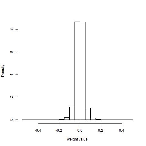
Figure 1: The histogram of the estimated weights of the four hidden layer DNN with MNIST data.

2.4 Remarks

Let ${\cal L}_{(l,j)}=\{{\bf x}:z_{j}^{(l)}({\bf x})=0\}$ be the boundary of the activation pattern, which we call the activation boundary, of the node $(l,j).$ Note that the gradient of $f({\bf x})$ changes only at ${\cal L}=\cup_{(l,j)\in{\cal I}}{\cal L}_{(l,j)}.$ Theorem 1 implies that the variation of gradient differences on ${\cal L}_{L\cdot}=\cup_{j}{\cal L}_{L,j}$ dominates the variation of gradient difference on the other boundaries provided $L=l_{*}.$ That is, when $n_{L}/n_{l}\rightarrow 0$ for all $l<L,$ we may ignore the variation of gradient differences at the activation boundaries corresponding to other than the highest layer and say that the function $f$ constructed by a deep neural network is mostly decided by the activation boundaries ${\cal L}_{L\cdot}$ made by the nodes at the highest layer and the variation of gradient differences on ${\cal L}_{L\cdot}.$ This argument suggests that we can approximate the function generated by a deep neural network by a nodewise linear function as

$$f({\bf x})\approx\beta_{0}+\sum_{j=1}^{n_{L}}\left\{\alpha_{j}+{\bf x}^{T}\nabla_{j}\right\}I(z_{j}^{(L)}({\bf x})\geq 0),$$ (3)

where $\nabla_{j}$ is the gradient difference at the boundary ${\cal L}_{Lj},j=1,\ldots,n_{L}.$ The role of the nodes at the intermediate layers is to increase the complexity of ${\cal L}_{L\cdot}$ as explained by Montufar et al. (2014) and Raghu et al. (2016).

A simpler version than (3) is

$$f({\bf x})\approx\beta_{0}+\sum_{j=1}^{n_{L}}\theta_{j}I(z_{j}^{(L)}({\bf x})\geq 0),$$ (4)

which is nodewise piecewise constant function rather than nodewise piecewise linear. In Section 3.2, we will show by analyzing real data that the approximation (4) works quite well for image classification tasks.

The approximation (4) amply explains why deep neural networks become more invariant to input transformation. Unless transformation of input does not change the activation pattern of the nodes at the highest layer, the function (4) does not change at all. The conclusion is that deep neural networks make the activation boundaries of the nodes at the highest layer be more complex and at the same time the variation of the function on the other activate boundaries be smaller. By doing so, deep neural networks can achieve complexity and transformation invariancy simultaneously.

3 Numerical Experiments

3.1 Experiments with DNN

In this section, we confirm the result of Theorem 1 with DNN architectures with randomly generated parameters as well as parameters learned based on MNIST data.

It is computationally infeasible to calculate all $\nabla^{2}_{(l,j),R},R\in{\cal R}.$ Alternatively, we investigate the variation of $f$ for a randomly selected path as is done by Raghu et al. (2016). For given two points ${\bf x}_{1}$ and ${\bf x}_{2},$ we let ${\bf x}(t)={\bf x}_{1}+t({\bf x}_{2}-{\bf x}_{1})$ for $t\in[0,1],$ which is the line connecting ${\bf x}_{1}$ and ${\bf x}_{2}.$ We investigate the variation of $g(t)=f({\bf x}_{1}+t({\bf x}_{2}-{\bf x}_{1})),t\in[0,1]$ for randomly selected ${\bf x}_{1}$ and ${\bf x}_{2}.$ Note that $g(t)$ is a piecewise linear function. Suppose that $g$ has nonzero gradient differences at $0=t_{0}<t_{1}<t_{2}<\cdots<t_{M}<t_{M+1}=1$ and let $\nabla^{2}_{m}=\nabla g(t_{m}+)-\nabla g(t_{m}-).$ Since each kinky point $t_{m}$ corresponds to a node $(l,j)$ such that ${\rm sign}\big{(}z^{(l)}_{j}(t_{m}+)\big{)}\neq{\rm sign}\big{(}z^{(l)}_{j}(t_{m}-)\big{)},$ where $z_{j}^{(l)}(t)=z_{j}^{(l)}\big{(}{\bf x}_{1}+t({\bf x}_{2}-{\bf x}_{1})\big{)},$ we denote such $(l,j)$ as $(l_{m},j_{m}).$ Since the value of $\nabla^{2}_{m}$ is proportional to $\|{\bf x}_{1}-{\bf x}_{2}\|,$ we normalize it to $\tilde{\nabla}_{m}^{2}=\nabla_{m}^{2}/\|{\bf x}_{1}-{\bf x}_{2}\|.$ We investigate the behaviors of $\tilde{\nabla}_{m}^{2}.$ In particular, we illustrate that the size of $\tilde{\nabla}_{m}^{2}$ becomes larger when the number of nodes in the layer $l_{m}$ becomes smaller. Whenever necessary, we write $\tilde{\nabla}_{m}^{2}({\bf x}_{1},{\bf x}_{2})$ to emphasize that $\tilde{\nabla}_{m}^{2}$ depends on ${\bf x}_{1}$ and ${\bf x}_{2}.$

First, we consider a DNN architecture with randomly generated parameters. For the fully connected DNN architecture, we set $p=784,L=4,(n_{1},n_{2},n_{3})=(1200,600,300)$ and study the behaviors of $f({\bf x})$ for various values of $n_{4}.$ For given ${\bf x}_{1},{\bf x}_{2}$ and $\theta,$ let ${\cal N}_{l}({\bf x}_{1},{\bf x}_{2},\theta)=\{||\tilde{\nabla}^{2}_{m}({\bf x}_{1},{\bf x}_{2})||_{2}:l_{m}=l\}$ for $l=1,\ldots,L.$ We generate the parameters $\theta^{(b)}$ and $({\bf x}_{1}^{(b)},{\bf x}_{2}^{(b)}),b=1,\ldots,100$ independently from the Gaussian distribution with mean 0 and variance 1 truncated on $[-1,1]$ to obtain ${\cal N}_{l}({\bf x}_{1}^{(b)},{\bf x}_{2}^{(b)},\theta^{(b)}),b=1,\ldots,B$ for $l=1,\ldots,4.$ Let ${\cal N}_{l}=\bigcup_{b}{\cal N}_{l}({\bf x}_{1}^{(b)},{\bf x}_{2}^{(b)},\theta^{(b)}).$ We normalize the gradient differences in $\cup_{l}{\cal N}_{l}$ to have the unit standard deviation for the sake of easy comparison.

Table 1 summarizes the cardinalities of ${\cal N}_{l}$ and the means of the absolute gradient differences in ${\cal N}_{l}$ for $l=1,\ldots,4,$ respectively. The cardinalities of ${\cal N}_{l}$ are proportional to the numbers of nodes $n_{l},$ which implies that all the nodes are equally activated/deactivated. The mean of the absolute gradient differences increases as the number of nodes at each layer decreases, which confirms Theorem 1.

	Layer
$n_{L}$	1	2	3	4
50	55.92	27.77	14.00	2.31
100	54.60	27.13	13.66	4.61
150	53.36	26.53	13.36	6.75

(a) The percentages of activated nodes at each layer (i.e. $100\times|{\cal N}_{l}|/\sum_{h=1}^{4}|{\cal N}_{h}|$)

	Layer
$n_{L}$	1	2	3	4
50	0.481	0.671	0.912	1.287
100	0.463	0.653	0.898	1.296
150	0.443	0.635	0.885	1.300

(b) Means of the absolute gradient differences at each layer

Table 1: The percentages of the numbers of the activated nodes and means of absolute values of gradient differences at each layer by the DNN with random parameters.

For MNIST data, we randomly select ${\bf x}_{1}$ and ${\bf x}_{2}$ but fix $\theta$ learned on the data. Since there are ten classes in the MNIST data, we select two classes “4” and “9”, which are known to be most difficult to classify, and investigate the behavior of the function $f_{9}({\bf x})-f_{4}({\bf x}),$ where $f_{k}({\bf x})$ is the value at the output node of class $k.$ We sample ${\bf x}_{1}$ and ${\bf x}_{2}$ randomly 100 times from the two classes respectively to obtain ${\cal N}_{l},l=1,\ldots,L.$ The results are summarized in Table 2 which are similar to those in Table 1 except that the results for the first and second layers are reversed. However, still the variation of gradient differences at the highest layer is the largest which reassures the main message of this paper.

	Layer
$n_{L}$	1	2	3	4
50	30.59	45.88	16.44	7.07
100	27.63	45.19	22.50	4.66
150	33.77	48.55	14.69	2.97

(a) The percentages of activated nodes at each layer (i.e. $100\times|{\cal N}_{l}|/\sum_{h=1}^{4}|{\cal N}_{h}|$)

	Layer
$n_{L}$	1	2	3	4
50	2.329	1.971	4.663	10.899
100	2.906	1.512	3.480	5.614
150	2.316	1.342	4.376	11.640

(b) Means of the absolute gradient differences at each layer

Table 2: The percentages of the numbers of the activated nodes and means of absolute values of gradient differences at each layer by the DNN learned on MNIST data

Figure 2 draws three paths of $g(t),t\in[0,1]$ for 3 randomly selected ${\bf x}_{1}$ and ${\bf x}_{2},$ where $g(t)=f_{9}({\bf x}_{1}+t({\bf x}_{2}-{\bf x}_{1}))-f_{4}({\bf x}_{1}+t({\bf x}_{2}-{\bf x}_{1})).$ A common feature in the three paths is that the gradient around $g(t)=0$ is the largest, which is helpful for transformation invariance because the output value does not change much except near the decision boundary.

In addition, we investigate which nodes are activated/deactivated around $g(t)=0.$ We find $t_{0}$ such that $g(t_{0})=0,$ and collect the nodes activated/deactivated in $(t_{0}-h,t_{0}+h).$ Table 3 presents the percentages of these activated/deactivated nodes for each layer. By comparing the results in Table 2 and Table 3, we can clearly see that much more nodes at the highest layer are activated/deactivated around the decision boundary.

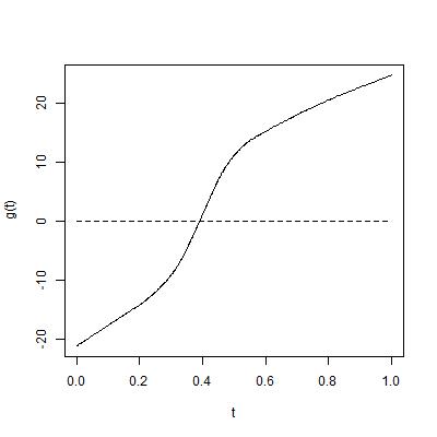
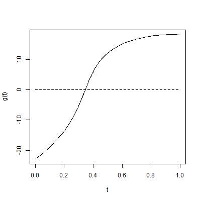
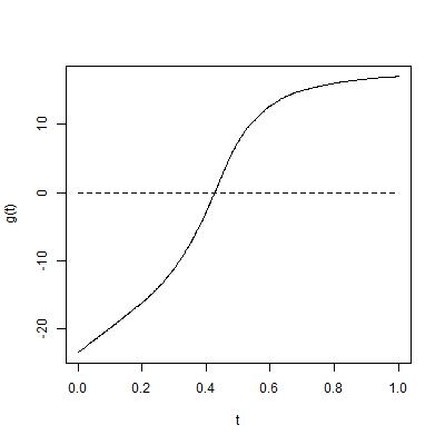
Figure 2: Three randomly selected paths of $g(t),t\in[0,1]$

	Layer
$n_{L}$	1	2	3	4
50	34.14	19.51	29.26	17.07
100	14.61	24.39	48.78	12.19
150	39.02	31.70	21.95	7.31

Table 3: The percentages of the numbers of the activated nodes at each layer around $(t_{0}-h,t_{0}+h)$

3.2 Experiments with CNN

We will show by analyzing the SVHN and CIFAR10 data that the approximation (4) in Section 2.4 performs quite well for image classification tasks with the CNN architecture. We use the architectures similar to those used in Miyato et al. (2017) except that the two fully connected layers are added at the highest layer, whose details are given in the supplementary material. We learned the architectures to have the activation pattern $I(z_{j}^{(L)}({\bf x})\geq 0),j=1,\ldots,n_{L}.$ Then, we let

$$\Pr(y=k|{\bf x})\propto\exp\left\{\theta_{k0}+\sum_{j=1}^{n_{L}}\theta_{kj}I(z_{j}^{(L)}({\bf x})\geq 0)\right\}$$ (5)

and learned the parameters $\theta_{k0}$ and $\theta_{kj}$ by minimizing the cross-entropy while the activation pattern $I\big{(}z_{j}^{(L)}({\bf x})\geq 0\big{)}$ being fixed. Table 4 compares the classwise accuracies of the approximated model based on (5) and the model based on the original architecture, which shows that the performances of the two models are fairly similar.

		class
		0	1	2	3	4	5	6	7	8	9	All
SVHN	CNN	96.8	97.1	97.6	94.5	97.2	96.4	96.3	96.4	94.0	95.4	96.39
	CNN-D	96.6	91.3	97.5	94.1	96.9	95.9	96.3	95.6	93.7	94.9	96.19
CIFAR10	CNN	89.1	95.5	84.4	73.8	89.3	82.8	92.5	91.7	94.5	93.2	88.68
	CNN-D	89.9	95.5	82.9	75.6	89.3	82.6	90.7	91.2	93.6	92.1	88.34

Table 4: Classwise accuracies of the original CNN architectures (CNN) and approximated models (CNN-D) by (5)

3.3 Experiments with semi-supervised learning

The purpose of semi-supervised learning is to improve accuracy by using not only small amount of labeled data but also large amount of unlabeled data. There are many recent researches about semi-supervised learning with deep neural networks including Salimans et al. (2016); Dai et al. (2017); Miyato et al. (2017).

One of the ideas of using unlabeled data is to locate the decision boundary on the areas where the density of unlabeled data is low (Grandvalet and Bengio, 2005). A similar idea can be applied to the activation boundaries made by the nodes at the highest layer. It would be beneficial to locate ${\cal L}_{L,j},j=1,\ldots,n_{L}$ on the areas where the density of unlabeled data is low. That is, we learn a given deep neural network such that most of unlabeled data locate far from the activation boundaries ${\cal L}_{L,j},j=1,\ldots,L.$ We have shown that most of large variations of $z_{j}^{(L)}({\bf x})$ occur near the activation boundaries ${\cal L}_{L,j}.$ Thus, we can expect that the variations of $z_{j}^{(L)}({\bf x})$ are relatively small when ${\bf x}$ is far from ${\cal L}_{L,j},$ which implies that $\left(z_{j}^{(L)}({\bf x})-z_{j}^{(L)}({\bf x}+\eta)\right)^{2}$ is relatively small for a random perturbation $\eta$ when ${\bf x}$ locates far from ${\cal L}_{L,j}.$ Based on this idea, the following regularization term would be helpful:

$$R(\theta)=\frac{1}{n_{u}}\sum_{i=1}^{n_{u}}\sum_{j=1}^{L}\left(z_{j}^{(L)}({\bf x}_{i}^{(u)})-z_{j}^{(L)}({\bf x}_{i}^{(u)}+\eta_{i})\right)^{2}$$

for given random perturbations $\eta_{i},i=1,\ldots,n_{u},$ where ${\bf x}_{i}^{(u)},i=1,\ldots,n_{u}$ are unlabeled data. We learn the parameter $\theta$ by minimizing $CE(\theta)+\lambda R(\theta),$ where $CE(\theta)$ is the cross-entropy of labeled data and $\lambda>0$ is a regularization parameter.

A similar idea has been used by Miyato et al. (2017), where the regularization term for unlabeled data is the KL divergence between the class probabilities of unlabeled and perturbed unlabeled data. We applied our method to MNIST and SVHN data and obtained similar accuracies to other competitors as shown in Table 5. The details of model architectures we used are given in the supplementary material. Even if our method does not dominate the others, however, the results amply support our theoretical finding that the activation boundaries of the nodes at the highest layer are most important for the success of deep neural networks. Note that the objective of this analysis is to support our theoretical result but not to develop a state-of-art semi-supervised learning algorithm. Note that the purpose this experiment is to confirm the utility of Theorem 1 but not develop a state-of-art semi-supervised learning algorithm.

Method	Test acc.($\%$)
	MNIST	SVHN
GAN with FM (Salimans et al., 2016)	99.07	91.89
Bad GAN (Dai et al., 2017)	99.20	95.75
VAT (Miyato et al., 2017)	98.64	93.17
Our method	97.92	93.22

Table 5: Test performances on MNIST (100 labeled data) and SVHN (1,000 labeled data) without data augmentation

4 Concluding Remarks

We have studied how the function constructed by a deep neural network with ReLU activation function behaves. In particular, we have shown that most of large variations of the function concentrate on the activation boundaries of the nodes at the highest layer and thus deep neural networks can achieve complexity and invariancy simultaneously. Our result can give a useful guide how to design a DNN architecture.

We only considered fully connected deep neural networks. Theoretical studies for other architectures including CNN, RNN and generative models need further studies. In particular, it would be interesting to explain the success of RNN since many successful RNN architectures use the tanh activation function rather than ReLU.

Our theoretical result could also provide a new direction for improving the interpretability of deep neural networks. The implication of our result is that we can focus only on the activation boundaries of the nodes at the highest layer. Visualization techniques for deep neural networks such as Montavon et al. (2017) could be modified for the activation boundary of the highest layer.

Appendix A Appendix

A.1 Proof of Proposition 1

Let $D_{j}^{(l)}=\partial\mathcal{A}_{R}\cap{\cal F}_{R,j}^{(l)}.$ Then $\partial\mathcal{A}_{R}=\cup_{(l,j)\in{\cal I}}D_{j}^{(l)}.$ Since $R^{\prime}$ is adjacent to $R,$ there exists $(l,j)$ such that $dim(D_{j}^{(l)}\cap\mathcal{A}_{R^{\prime}})=p-1.$ Otherwise, $dim(\partial\mathcal{A}_{R}\cap\partial\mathcal{A}_{R^{\prime}})$ cannot be $p-1.$ Let $(l,j)$ be an index such that $dim(D_{j}^{(l)}\cap\mathcal{A}_{R^{\prime}})=p-1.$ Since $\theta$ is simple, we can choose ${\bf x}\in D_{j}^{(l)}\cap\mathcal{A}_{R^{\prime}}$ and $\epsilon$ such that $B({\bf x}:\epsilon)\cap\mathcal{A}_{R}\neq\emptyset,B({\bf x}:\epsilon)\cap\mathcal{A}_{R^{\prime}}\neq\emptyset$ and $B({\bf x}:\epsilon)\cap{\cal F}_{(l^{\prime},j^{\prime})}=\emptyset$ for all $(l^{\prime},j^{\prime})\neq(l,j),$ where $B({\bf x}:\epsilon)=\{{\bf y}\in\mathbb{R}^{p}:\|{\bf x}-{\bf y}\|<\epsilon\}.$ Hence, there exist ${\bf x}_{1}\in\mathcal{A}_{R}$ and ${\bf x}_{2}\in\mathcal{A}_{R^{\prime}}$ such that ${\rm sign}\big{(}z_{j^{\prime}}^{(l^{\prime})}({\bf x}_{1}:\theta)\big{)}={\rm sign}\big{(}z_{j^{\prime}}^{(l^{\prime})}({\bf x}_{2}:\theta)\big{)}$ for all $(l^{\prime},j^{\prime})\neq(l,j)$ and ${\rm sign}\big{(}z_{j}^{(l)}({\bf x}_{1}:\theta)\big{)}\neq{\rm sign}\big{(}z_{j}^{(l)}({\bf x}_{2}:\theta)\big{)},$ and hence the proof is done. $\square$

A.2 Proof of Theorem 1

We start with two technical lemmas.

Lemma 1

Suppose $Z_{1},\ldots,Z_{m}$ be continuous random variables having the second moment such that

$$(Z_{1},\ldots,Z_{m})\stackrel{{\scriptstyle d}}{{=}}(-Z_{1},\ldots,-Z_{m}).$$

For given constants $a_{1},\ldots,a_{m}$ and $b_{1},\ldots,b_{m},$ let $X=\sum_{j=1}^{m}a_{j}Z_{j}$ and $Y=\sum_{j=1}^{m}b_{j}Z_{j}.$ Then

$$E(X^{2}I(Y>0))=E(X^{2})/2.$$

Proof. Note that $X^{2}I(Y>0)\stackrel{{\scriptstyle d}}{{=}}X^{2}I(Y<0).$ Since $X^{2}=X^{2}I(Y>0)+X^{2}I(Y<0),$ the proof is done. $\square$

Lemma 2

Let $\mathcal{R}=\{R({\bf x}):{\bf x}\in\mathbb{R}^{n_{0}}\}$ be the set of all activation patterns. Then $|\mathcal{R}|=O(\prod_{l=1}^{L}n_{l}^{n_{0}})$.

Proof. Let $\mathcal{R}_{l}$ be the set of all activation patterns of $f_{l}({\bf x})={\bf h}^{(l)}({\bf x})$. By Zaslavsky’s theorem [Stanley et al., 2004], $\mathcal{R}_{1}\leq\sum_{s=0}^{n_{0}}{n_{1}\choose k}=$, and in turn $\sum_{s=0}^{n_{0}}{n_{1}\choose k}=O(n_{1}^{n_{0}}).$. By applying this result repeatedly, we have $|\mathcal{R}|=O(\prod_{l=1}^{L}n_{l}^{n_{0}})$. $\square$

For national simplicity, we consider $-1$th and $(L+1)$th layers with $n_{-1}=1,w^{(0)}_{j1}=v_{j},R^{(-1)}_{1}=1$ and $n_{L+1}=1,w^{(L+1)}_{1j}=\beta_{j},R^{(L+1)}_{1}=1.$ Also, we let $R_{j}^{(0)}=1$ for $j=1,\ldots,n_{0}.$ Let $N=\prod_{l=0}^{L}n_{l}$ and $\mu_{k}=E(\xi^{k})$ where $\xi$ is a random variable whose distribution function is $G$.

For $l<l^{\prime}$ let

$${\cal P}_{(l,j),(l^{\prime},j^{\prime})}=\{(j,r_{l+1}\ldots,r_{l^{\prime}-1},j^{\prime}):r_{h}=1,\ldots,n_{h},h=l+1,\ldots,l^{\prime}-1\}.$$

Define $V_{(l,j),(l^{\prime},j^{\prime})}$ as

$$V_{(l,j),(l^{\prime},j^{\prime}),R}=\sum_{r\in{\cal P}_{(l,j),(l^{\prime},j^{\prime})}}W_{r}R_{r}$$

where $W_{r}=\prod_{i=2}^{|r|}w_{r_{i},r_{i-1}}^{(l+i-1)}$ and $R_{r}=\prod_{i=2}^{|r|}R_{r_{i}}^{(l+i-1)},$ where $|r|$ is the dimension of a vector $r.$ Then, we can write

$${\bf v}^{T}\nabla^{2}_{(l,j),R}=V_{(l,j),(L+1,1),R}V_{(-1,1),(l,j),R}$$

Let $\theta_{l}=(b^{(l)}_{j},w^{(l)}_{j,j^{\prime}},j=1,\ldots,n_{l},j^{\prime}=1,\ldots,n_{l-1})$ and let ${\cal F}_{l}=\sigma(\theta_{1},\ldots,\theta_{l})$ be the $\sigma$-field generated by $\theta_{1},\ldots,\theta_{l}.$

A.2.1 Upper bound

Let $U_{(l,j),(l^{\prime},j^{\prime}),R}=V_{(l,j),(l^{\prime},j^{\prime}),R}$ for $l^{\prime}=l+1$ and

$$U_{(l,j),(l^{\prime},j^{\prime}),R}=\frac{V_{(l,j),(l^{\prime},j^{\prime}),R}}{\sqrt{n_{l+1}\cdots n_{l^{\prime}-1}}}$$

for $l^{\prime}\geq l+2.$ For given constants $c_{n,l},$ which are specified later, we let

$${\cal B}_{l}=\bigcap_{j=1}^{n_{l}}\bigcap_{(l^{\prime},j^{\prime})\in{\cal I}_{l-1}}\bigcap_{R\in{\cal R}}\left\{|U_{(l^{\prime},j^{\prime}),(l,j),R}|\leq c_{n,l}\mbox{ for all }{\bf v}\in[-1,1]^{n_{0}}\right\},$$

where ${\cal I}_{l}=\{(l^{\prime},j^{\prime}):l^{\prime}=-1,\ldots,l,j^{\prime}=1,\ldots,n_{l^{\prime}}\}.$ We will derive the constants $c_{n,l}$ such that $\Pr\{{\cal B}_{l}^{c}\}\rightarrow 0$ for $l=1,\ldots,L+1.$

Consider the case of $l=1.$ Then ${\cal B}_{1}={\cal B}_{11}\cap{\cal B}_{12},$ where

$${\cal B}_{11}=\bigcap_{j=1}^{n_{1}}\bigcap_{R\in{\cal R}}\{|U_{(-1,1),(1,j),R}|\leq c_{n,1}\mbox{ for all }{\bf v}\in[-1,1]^{n_{0}}\}$$

and

$${\cal B}_{12}=\bigcap_{j=1}^{n_{1}}\bigcap_{j^{\prime}=1}^{n_{0}}\bigcap_{R\in{\cal R}}\{|U_{(0,j^{\prime}),(1,j),R}|\leq c_{n,1}\}.$$

Since $|U_{(0,j^{\prime}),(1,j),R}|=|w^{(1)}_{j,j^{\prime}}R_{j}^{(1)}|\leq\tau,$ $\Pr\{{\cal B}_{12}\}=1$ if $c_{n,1}\geq\tau.$ Hence $\Pr\{{\cal B}_{1}\}=\Pr\{{\cal B}_{11}\}.$ Note that $|U_{(-1,1),(1,j),R}|=\left|R_{j}^{(1)}\frac{\sum_{j^{\prime}=1}^{n_{0}}w_{j,j^{\prime}}^{(1)}v_{j}}{\sqrt{n_{0}}}\right|\leq\left|\frac{\sum_{j^{\prime}=1}^{n_{0}}w_{j,j^{\prime}}^{(1)}v_{j}}{\sqrt{n_{0}}}\right|.$ Since $\frac{\sum_{j^{\prime}=1}^{n_{0}}w_{j,j^{\prime}}^{(1)}v_{j}}{\sqrt{n_{0}}}$ is a linear function of ${\bf v}$,

$$\left\{\left|\frac{\sum_{j^{\prime}=1}^{n_{0}}w_{j,j^{\prime}}^{(1)}v_{j}}{\sqrt{n_{0}}}\right|\leq c_{n,1}\mbox{ for all }{\bf v}\in[-1,1]^{n_{0}}\right\}=\left\{\left|\frac{\sum_{j^{\prime}=1}^{n_{0}}w_{j,j^{\prime}}^{(1)}v_{j}}{\sqrt{n_{0}}}\right|\leq c_{n,1}\mbox{ for all }{\bf v}\in{\cal V}\right\},$$

where ${\cal V}=\{-1,1\}^{n_{0}}$. Thus we have

$${\cal B}_{11}\supset\bigcap_{j=1}^{n_{1}}\bigcap_{R\in{\cal R}}\left\{\left|\frac{\sum_{j^{\prime}=1}^{n_{0}}w_{j,j^{\prime}}^{(1)}v_{j}}{\sqrt{n_{0}}}\right|\leq c_{n,1}\mbox{ for all }{\bf v}\in{\cal V}\right\}.$$

Thus

$$\Pr({\cal B}_{11}^{c})\leq\sum_{j=1}^{n_{1}}\sum_{{\bf v}\in{\cal V}}\Pr\left\{\left|\frac{\sum_{j^{\prime}=1}^{n_{0}}w_{j,j^{\prime}}^{(1)}v_{j}}{\sqrt{n_{0}}}\right|>c_{n,1}\right\}.$$

By Hoeffiding’s inequality,

$$\Pr\left\{\left|\frac{\sum_{j^{\prime}=1}^{n_{0}}w_{j,j^{\prime}}^{(1)}v_{j}}{\sqrt{n_{0}}}\right|>c_{n,1}\right\}\leq 2\exp\left(-\frac{c_{n,1}^{2}}{2\tau^{2}}\right),$$

and hence

$$\Pr({\cal B}_{1}^{c})\leq 2n^{\alpha_{1}}c_{v}\exp\left(-\frac{c_{n,1}^{2}}{2\tau^{2}}\right),$$

where $c_{v}=|{\cal V}|.$

For general $l>1,$ we write ${\cal B}_{l}={\cal B}_{l1}\cap{\cal B}_{l2},$ where

$${\cal B}_{l1}=\bigcap_{j=1}^{n_{l}}\bigcap_{(l^{\prime},j^{\prime})\in{\cal I}_{l-2}}\bigcap_{R\in{\cal R}}\left\{|U_{(l^{\prime},j^{\prime}),(l,j),R}|\leq c_{n,l}\mbox{ for all }{\bf v}\in[-1,1]^{n_{0}}\right\}$$

and

$${\cal B}_{l2}=\bigcap_{j=1}^{n_{l}}\bigcap_{j^{\prime}=1}^{n_{l-1}}\bigcap_{R\in{\cal R}}\left\{|U_{(l-1,j^{\prime}),(l,j),R}|\leq c_{n,l}\right\}.$$

Similarly to ${\cal B}_{1,2},$ we can show that $\Pr\{{\cal B}_{l2}\}=1$ if $c_{n,l}\geq\tau.$ Also, similarly to ${\cal B}_{11},$ we have

$${\cal B}_{l1}=\bigcap_{j=1}^{n_{l}}\bigcap_{(l^{\prime},j^{\prime})\in{\cal I}_{l-2}}\bigcap_{R\in{\cal R}}\bigcap_{v\in{\cal V}}\left\{\left|\frac{\sum_{j^{\prime\prime}=1}^{n_{l-1}}w_{j,j^{\prime}}^{(l)}U_{(l^{\prime},j^{\prime}),(l-1,j^{\prime\prime}),R}}{\sqrt{n_{l-1}}}\right|\leq c_{n,l}\right\},$$

and so

$$\Pr\{{\cal B}_{l}^{c}\}\leq\sum_{j=1}^{n_{l}}\sum_{(l^{\prime}j^{\prime})\in{\cal I}_{l-2}}\sum_{R\in{\cal R}}\sum_{{\bf v}\in{\cal V}_{\delta}}\Pr\left\{\left|\frac{\sum_{j^{\prime\prime}=1}^{n_{l-1}}w_{j,j^{\prime}}^{(l)}U_{(l^{\prime},j^{\prime}),(l-1,j^{\prime\prime}),R}}{\sqrt{n_{l-1}}}\right|>c_{n,l}\right\}.$$

Note that $w_{j,j^{\prime}}^{(l)}$ and $U_{(l^{\prime},j^{\prime}),(l-1,j^{\prime\prime}),R}$ are independent. Hence, Hoeffiding’s inequality implies that

$$\Pr\left\{\left|\frac{\sum_{j^{\prime\prime}=1}^{n_{l-1}}w_{j,j^{\prime}}^{(l)}U_{(l^{\prime},j^{\prime}),(l-1,j^{\prime\prime}),R}}{\sqrt{n_{l-1}}}\right|>c_{n,l}\left.\rule{0.0pt}{18.06749pt}\right|{\cal F}_{l-1}\right\}\leq 2\exp\left(-\frac{c_{n,l}^{2}}{2\tau^{2}\sigma^{2}}\right),$$

where

$$\sigma^{2}=\frac{1}{n_{l-1}}\sum_{j^{\prime\prime}=1}^{n_{l-1}}U^{2}_{(l^{\prime},j^{\prime}),(l-1,j^{\prime\prime}),R}.$$

By the definition of ${\cal B}_{l-1}$ and Lemma 2, we have

$$\Pr({\cal B}_{l}^{c}) \leq n^{\alpha_{l}}n^{\alpha_{1:(l-2)}}n_{0}|{\cal R}|c_{v}\left(2\exp\left(-\frac{c_{n,l}^{2}}{2\tau^{2}c_{n,l-1}^{2}}\right)+\Pr({\cal B}_{l-1}^{c})\right),$$ (6)

$$= O(n^{2\cdot\alpha^{1:l}})n_{0}c_{v}\left(2\exp\left(-\frac{c_{n,l}^{2}}{2\tau^{2}c_{n,l-1}^{2}}\right)+\Pr({\cal B}_{l-1}^{c})\right)$$

where $\alpha_{1:l}=\alpha_{1}+\cdots+\alpha_{l}.$

By applying (6) repeatedly, we have

$$\Pr\{{\cal B}_{L+1}^{c}\} \leq O(n^{2\cdot\alpha^{1:(L+1)}})n_{0}c_{v}\left(2\exp\left(-\frac{c_{n,L+1}^{2}}{2\tau^{2}c_{n,L}^{2}}\right)+\Pr({\cal B}_{L}^{c})\right)$$

$$\leq O(n^{2\cdot\alpha^{1:(L+1)}})n_{0}c_{v}2\exp\left(-\frac{c_{n,L+1}^{2}}{2\tau^{2}c_{n,L}^{2}}\right)$$

$$+O(n^{2\cdot\alpha^{1:(L+1)}})O(n^{2\cdot\alpha^{1:L}})(n_{0}c_{v})^{2}\left(2\exp\left(-\frac{c_{n,L}^{2}}{2\tau^{2}c_{n,L-1}^{2}}\right)+\Pr({\cal B}_{L-1}^{c})\right)$$

$$\leq \cdots$$

$$\leq \sum_{l=1}^{L+1}O(n^{\gamma_{l}})(n_{0}c_{v})^{L+2}\cdot 2\exp\left(-\frac{c_{n,l}^{2}}{2\tau^{2}c_{n,l-1}^{2}}\right)$$

with $c_{n,0}=1$ for some positive integers $\gamma_{l},l=1,\ldots,L+1.$ Hence, we can choose positive constants $\nu_{l},l=1,\ldots,L+1,$ such that $\Pr\{{\cal B}_{l}^{c}\}\rightarrow 0$ with $c_{n,l}=\nu_{l}(\log n)^{2l-1}$ for $l=1,...,L+1$.

An obvious corollary of $\Pr\{{\cal B}_{L+1}^{c}\}\rightarrow 0$ is that

$$\sup_{(l,j),R\in{\cal R},{\bf v}\in[-1,1]^{n_{0}}}\sqrt{n_{l}}\frac{{\bf v}^{T}\nabla^{2}_{(l,j),R}}{\sqrt{N}}=O_{p}\left((\log n)^{4L-2}\right).$$ (7)

A.2.2 Lower bound

We fix ${\bf v}\in[-1,1]^{n_{0}}$ with $\|{\bf v}\|=1$ and ${\bf x}\in{\cal X}.$ Let $0<c<\tau$ be a constant and

$${\cal L}_{*}=\left\{\theta:\max_{j=1,\ldots,n_{*}}\sqrt{n_{l_{*}}}\left|\frac{{\bf v}^{T}\nabla^{2}_{(l_{*},j),R({\bf x})}}{\sqrt{N}}\right|\geq c\right\}.$$

We will show that

$$\Pr\{{\cal L}_{*}\}\rightarrow 1.$$ (8)

We will prove (8) for $l_{*}=L.$ A similar technique can be used to prove the other cases. Note that

$$\sqrt{n_{l_{*}}}\frac{{\bf v}^{T}\nabla^{2}_{(l_{*},j),R({\bf x})}}{\sqrt{N}}=\beta_{j}U_{(-1,1),(L,j),R({\bf x})}.$$

By abusing the notations slightly, we write $U_{(-1,1),(l,j),R(x)}$ as $U_{l,j}.$ We divide the proof into the three steps.

[Step 1] Define ${\cal M}_{l}(\gamma)$ as

$${\cal M}_{l}(\gamma)=\left\{\left|\frac{1}{n_{l}}\sum_{j=1}^{n_{l}}\left\{U_{l,j}^{2}-\mbox{{\rm E}}(U^{2}_{l,j}|{\cal F}_{l-1})\right\}\right|\leq\gamma\right\}.$$

We first show that

$$\Pr({\cal M}_{l}(\gamma))\rightarrow 1$$ (9)

for all $l$ and any $\gamma>0.$ Note that $U_{l,j},j=1,\ldots,n_{l}$ are independent conditional on ${\cal F}_{l-1}.$ Hence, Chebyshev’s inequality implies that

$$\Pr\left\{\left|\frac{1}{n_{l}}\sum_{j=1}^{n_{l}}\left\{U_{l,j}^{2}-\mbox{{\rm E}}(U^{2}_{l,j}|{\cal F}_{l-1})\right\}\right|>\gamma\left.\rule{0.0pt}{18.06749pt}\right|{\cal F}_{l-1}\right\}\leq\frac{\sum_{j=1}^{n_{l}}\mbox{{\rm E}}\left[\left\{U_{l,j}^{2}-\mbox{{\rm E}}(U^{2}_{l,j}|{\cal F}_{l-1})\right\}^{2}|{\cal F}_{l-1}\right]}{n_{l}^{2}\gamma^{2}}.$$

By using $U_{l,j}=\left(\frac{R_{j}^{(l)}}{\sqrt{n_{l-1}}}\sum_{j^{\prime}=1}^{n_{l-1}}w_{j,j^{\prime}}^{(l)}U_{(l-1),j^{\prime}}\right)^{2}$, $U_{(l-1),j^{\prime}}\in{\cal F}_{l-1}$ and $w_{j,j^{\prime}}^{(l)}\perp{\cal F}_{l-1}$, we have the following equality on ${\cal B}_{l-1}$:

$$\mbox{{\rm E}}\left[\left\{U_{l,j}^{2}-\mbox{{\rm E}}(U^{2}_{l,j}|{\cal F}_{l-1})\right\}^{2}|{\cal F}_{l-1}\right] = \mbox{{\rm E}}\left[U_{l,j}^{4}|{\cal F}_{l-1}\right]-2\mbox{{\rm E}}\left[U_{l,j}^{2}|{\cal F}_{l-1}\right]^{2}$$

$$= \frac{R_{j}^{(l)}}{n_{l-1}^{2}}\left[(\mu_{4}-\mu_{2}^{2})\sum_{j^{\prime}=1}^{n_{l-1}}U_{(l-1),j^{\prime}}^{4}+2\mu_{2}^{2}\sum_{j^{\prime}\neq j^{\prime\prime}}U_{(l-1),j^{\prime}}^{2}U_{(l-1),j^{\prime\prime}}^{2}\right]$$

$$= O((\log n)^{4\cdot(2l-1)})$$

since $\sup_{j=1,\ldots,n_{l}}|U_{l,j}|\leq O\big{(}(\log n)^{2l-1}\big{)}$ on ${\cal B}_{l-1}$. Thus, we can easily check

$$\frac{\sum_{j=1}^{n_{l}}\mbox{{\rm E}}\left[\left\{U_{l,j}^{2}-\mbox{{\rm E}}(U^{2}_{l,j}|{\cal F}_{l-1})\right\}^{2}\right]}{n_{l}^{2}\gamma^{2}}\rightarrow 0$$

as $n\rightarrow\infty,$ and hence $\Pr\{{\cal M}_{l}(\gamma)\}\rightarrow 1.$

[Step 2] For given positive constants $\delta_{l},l=1,\ldots,L,$ define ${\cal U}_{l}$ by

$${\cal U}_{l}=\left\{\theta:\frac{1}{n_{l}}\sum_{j=1}^{n_{l}}U_{l,j}^{2}\geq\delta_{l}\right\}.$$

We will show that there exist positive constant $\delta_{l}$ such that

$$\Pr\{{\cal U}_{l}\}\rightarrow 1$$ (10)

for $l=1,\ldots,L.$

Consider the case of $l=1.$ Note that

$$U^{2}_{1,j}=I\left(\frac{R_{j}^{(1)}\sum_{j^{\prime}=1}^{n_{0}}w_{j,j^{\prime}}^{(1)}v_{j^{\prime}}}{\sqrt{n_{0}}}\right)^{2},$$

where $R_{j}^{(1)}=\big{(}b_{j}^{(1)}+\sum_{j^{\prime}=1}^{n_{0}}w_{j,j^{\prime}}^{(1)}x_{j}\geq 0\big{)}.$ By Lemma 1,

$$\mbox{{\rm E}}\left(\frac{R_{j}^{(1)}\sum_{j^{\prime}=1}^{n_{0}}w_{j,j^{\prime}}^{(1)}v_{j^{\prime}}}{\sqrt{n_{0}}}\right)^{2}=\frac{1}{2}\mbox{{\rm E}}\left(\frac{\sum_{j^{\prime}=1}^{n_{0}}w_{j,j^{\prime}}^{(1)}v_{j^{\prime}}}{\sqrt{n_{0}}}\right)^{2}=\mu_{2}/2,$$

and thus

$$\frac{\sum_{j=1}^{n_{1}}\mbox{{\rm E}}(U_{1,j}^{2})}{n_{1}}=\mu_{2}/2.$$

Therefore, ${\cal U}_{1}\supset{\cal M}_{1}(\gamma)$ if we let $\delta_{1}=\mu_{2}/2-\gamma,$ and so (10) holds with $\delta_{1}=\mu_{2}/2-\gamma.$

Suppose that (10) holds for $l-1.$ Note that

$$U^{2}_{l,j}=\left(\frac{R_{j}^{(l)}\sum_{j^{\prime}=1}^{n_{l-1}}w_{j,j^{\prime}}^{(l)}U_{(l-1),j^{\prime}}}{\sqrt{n_{l-1}}}\right)^{2},$$

where $R_{j}^{(l)}=I\big{(}b_{j}^{(l)}+\sum_{j^{\prime}=1}^{n_{l-1}}w_{j,j^{\prime}}^{(l)}U_{l-1,j^{\prime}}({\bf x})\geq 0\big{)}.$ By Lemma 1,

$$\mbox{{\rm E}}(U^{2}_{l,j}|{\cal F}_{l-1})=\frac{\mu_{2}}{2}\sum_{j^{\prime}=1}^{n_{l-1}}U_{l-1,j^{\prime}}^{2}.$$

Hence, ${\cal U}_{l}\cap{\cal U}_{l-1}\supset{\cal M}_{l}(\gamma)\cap{\cal U}_{l-1}$ with $\delta_{l}=\mu_{2}\delta_{l-1}n_{l-1}/2-\gamma.$ Since $\Pr\{{\cal M}_{l}(\gamma)\cap{\cal U}_{l-1}\}\rightarrow 1,$ (10) holds.

Finally, we can choose $\gamma$ satisfying $\delta_{l}>0$ for $l=1,\ldots,L$ and the proof of (10) is complete.

[Step 3] Let

$$\tilde{U}_{L,j}=\frac{1}{\sqrt{n_{L-1}}}\sum_{j^{\prime}=1}^{n_{L-1}}w_{j,j^{\prime}}^{(L)}U_{L-1,j}$$

and note that

$$\Pr\left\{\max_{j=1,\ldots,n_{L}}|\beta_{j}U_{L,j}|\leq c\left.\rule{0.0pt}{18.06749pt}\right|{\cal F}_{L}\right\}=\prod_{j=1}^{n_{L}}\left\{G\left(\frac{c}{|\tilde{U}_{L,j}|}\right)-G\left(-\frac{c}{|\tilde{U}_{L,j}|}\right)\right\}^{I(R_{j}^{(l)}=1)}$$ (11)

since $U_{L,j}=R_{j}^{(l)}\tilde{U}_{L,j}$. The Berry-Esseen theorem implies that there exists a universal constant $C>0$ such that

$$\Pr\{\tilde{U}_{L,j}\leq 1|{\cal F}_{L-1}\}\leq\Phi(1|\sigma_{j}^{2})+\frac{C}{\sqrt{n_{L-1}}}\frac{\rho_{j}}{(\sigma_{j}^{2})^{3/2}},$$

where $\Phi(\cdot|\sigma^{2})$ is the Gaussian distribution with mean 0 and variance $\sigma^{2},$

$$\sigma_{j}^{2}=\frac{\mu_{2}}{n_{L-1}}\sum_{j=1}^{n_{L-1}}U_{L-1,j}^{2}$$

and

$$\rho_{j}=\frac{\mu_{3}}{n_{L-1}}\sum_{j=1}^{n_{L-1}}|U_{L-1,j}|^{3}.$$

On ${\cal B}_{L-1}\cap{\cal U}_{L-1},$ we have

$$\Pr\left\{\tilde{U}_{L,j}\leq 1|{\cal F}_{L-1}\right\}=\Phi(1|\delta_{L-1})+o(1).$$

Note that $\tilde{U}_{L,j},j=1,\ldots,n_{L}$ are independent on ${\cal F}_{L-1},$ and hence on ${\cal B}_{L-1}\cap{\cal U}_{L-1},$

$$\Pr\left\{\max_{j=1,\ldots,n_{L}}\tilde{U}_{L,j}\leq 1\left.\rule{0.0pt}{18.06749pt}\right|{\cal F}_{L-1}\right\}\leq\left\{\Phi(1|\delta_{L-1})+o(1)\right\}^{n_{L}}\rightarrow 0.$$

Since $\Pr\{{\cal B}_{L-1}\cap{\cal U}_{L-1}\}\rightarrow 1,$ we have

$$\Pr\left\{\max_{j=1,\ldots,n_{L}}\tilde{U}_{L,j}>1\right\} \geq 1-\left[\left\{\Phi(1|\delta_{L-1})+o(1)\right\}^{n_{L}}\cdot\Pr\{{\cal B}_{L-1}\cap{\cal U}_{L-1}\}+\Pr\{{\cal B}_{L-1}^{c}\cup{\cal U}_{L-1}^{c}\}\right]$$ (12)

$$\rightarrow 1.$$

By using (11),

$$\Pr\left\{\max_{j=1,\ldots,n_{L}}|\beta_{j}U_{L,j}|\leq c\right\}=\mbox{{\rm E}}\left[\Pr\left\{\max_{j=1,\ldots,n_{L}}|\beta_{j}U_{L,j}|\leq c\left.\rule{0.0pt}{18.06749pt}\right|{\cal F}_{L}\right\}\right]$$

$$\leq \int_{max|\tilde{U}_{L,j}|>1}\prod_{j=1}^{n_{L}}\left\{G\left(\frac{c}{|\tilde{U}_{L,j}|}\right)-G\left(-\frac{c}{|\tilde{U}_{L,j}|}\right)\right\}^{I(R_{j}^{(L)}=1)}dP+P\left\{\max_{j=1,...,n_{L}}|\tilde{U}_{L,j}|\leq 1\right\}$$

$$\leq \mbox{{\rm E}}\left[\prod_{j=1}^{n_{L}}\left\{G(c)-G(-c)\right\}^{I(R_{j}^{(L)}=1)}\right]+P\left\{\max_{j=1,...,n_{L}}|\tilde{U}_{L,j}|\leq 1\right\}.$$

The second term of RHS for the above formula converges to 0 since (12) holds. Note that

$$\mbox{{\rm E}}\left[\prod_{j=1}^{n_{L}}\left\{G(c)-G(-c)\right\}^{I(R_{j}^{(L)}=1)}\left.\rule{0.0pt}{18.06749pt}\right|{\cal F}_{L-1}\right] = \prod_{j=1}^{n_{L}}\mbox{{\rm E}}\left[\left\{G(c)-G(-c)\right\}^{I(R_{j}^{(L)}=1)}\left.\rule{0.0pt}{18.06749pt}\right|{\cal F}_{L-1}\right]$$

$$= \prod_{j=1}^{n_{L}}\left[\frac{1}{2}\left(G(c)-G(-c)\right)+\frac{1}{2}\right]^{n_{L}},$$

and thus we achieve that the first term of RHS also converges to 0 for any positive constant $c<\tau$. As a result, we have

$$\Pr\left\{\max_{j=1,\ldots,n_{L}}|\beta_{j}U_{L,j}|\geq c\right\}\rightarrow 1$$

for any positive constant $c<\tau$ and hence the proof of (8) is done.

A.2.3 Proof of Theorem 1

Let ${\cal D}_{l}=\{\nabla^{2}_{(l,j),R},j=1,\ldots,n_{l},R\in{\cal R}\}$ for $l=1,\ldots,L.$ We have shown in (7) of Section A.2.1 that

$$\sup_{l\neq l^{*}}\sup_{{\bf d}\in{\cal D}_{l}}\sup_{{\bf v}\in[-1,1]^{n_{0}}}\frac{\sqrt{n_{l}}}{\sqrt{N}}|{\bf v}^{T}{\bf d}|=O_{p}\left((\log n)^{4L-2}\right).$$

Hence, by letting ${\bf v}={\bf d}/\|{\bf d}\|,$ we have

$$\sup_{l\neq l^{*}}\sup_{{\bf d}\in{\cal D}_{l}}\|{\bf d}\|=O_{p}\left(\frac{\sqrt{N}}{\min_{l\neq l^{*}}\sqrt{n_{l}}}(\log n)^{4L-2}\right).$$ (13)

On the other hand, we have proved in Section A.2.2 that

$$\Pr\left\{\frac{\sqrt{n_{*}}}{\sqrt{N}}|{\bf v}^{T}{\bf d}|>c\mbox{ for some }{\bf d}\in{\cal D}_{l_{*}}\right\}\rightarrow 1$$

as $n\rightarrow\infty,$ provided that $\|{\bf v}\|=1.$ Note that $|{\bf v}^{T}{\bf d}|\leq\|{\bf d}\|.$ Hence, we have

$$\max_{{\bf d}\in{\cal D}_{l_{*}}}\|{\bf d}\|\succ O_{p}\left(\frac{\sqrt{N}}{\sqrt{n_{*}}}\right),$$ (14)

where $a_{n}\succ b_{n}$ means $\liminf a_{n}/b_{n}>0.$ By combining (13) and (14), we complete the final property:

$$\frac{\max_{{\bf d}\in\cup_{l\neq l_{*}}{\cal D}_{l}}\|{\bf d}\|}{\max_{{\bf d}\in{\cal D}_{l_{*}}}\|{\bf d}\|}=O_{p}\left(\frac{\sqrt{n_{*}}}{\min_{l\neq l_{*}}\sqrt{n_{l}}}(\log n)^{4L-2}\right).$$

A.3 Experiments with CNN : model architectures

SVHN	CIFAR10
$32\times 32$ RGB images
$3\times 3$ conv. 64 ReLU	$3\times 3$ conv. 96 ReLU
$3\times 3$ conv. 64 ReLU	$3\times 3$ conv. 96 ReLU
$3\times 3$ conv. 64 ReLU	$3\times 3$ conv. 96 ReLU
$2\times 2$ max-pool, stride 2
dropout, $p=0.5$
$3\times 3$ conv. 128 ReLU	$3\times 3$ conv. 192 ReLU
$3\times 3$ conv. 128 ReLU	$3\times 3$ conv. 192 ReLU
$3\times 3$ conv. 128 ReLU	$3\times 3$ conv. 192 ReLU
$2\times 2$ max-pool, stride 2
dropout, $p=0.5$
$3\times 3$ conv. 128 ReLU	$3\times 3$ conv. 192 ReLU
$1\times 1$ conv. 128 ReLU	$1\times 1$ conv. 192 ReLU
$1\times 1$ conv. 128 ReLU	$1\times 1$ conv. 192 ReLU
global average pool, $6\times 6\to 1\times 1$
$128\times 128$ FC	$192\times 192$ FC
$128\times 128$ FC	$192\times 192$ FC
dense $128\to 10$	dense $192\to 10$
10-way softmax

Table 6: CNN models used in our experiments over SVHN and CIFAR-10. All the conv. layers and fully-connected layers are followed by BN.[Ioffe and Szegedy, 2015]

A.4 Semi-supervised learning : model architectures

For MNIST dataset, we used NN with five hidden layers, whose numbers of nodes were (1200,600,300,150,150). All the fully-connected layers are followed by BN[Ioffe and Szegedy, 2015]. And for SVHN dataset, we used the CNN model which is mentioned in Table 6. Note that our regularization term is variant to the scale of the highest node values, so we added normalization operation to the highest hidden layer for each architecture.

References

- Dai et al. [2017] Zihang Dai, Zhilin Yang, Fan Yang, William W Cohen, and Ruslan R Salakhutdinov. Good semi-supervised learning that requires a bad gan. In Advances in Neural Information Processing Systems, pages 6513–6523, 2017.
- Eldan and Shamir [2016] Ronen Eldan and Ohad Shamir. The power of depth for feedforward neural networks. In Conference on Learning Theory, pages 907–940, 2016.
- Fukuda et al. [1991] Komei Fukuda, Shigemasa Saito, Akihisa Tamura, and Takeshi Tokuyama. Bounding the number of k-faces in arrangements of hyperplanes. Discrete Applied Mathematics, 31(2):151–165, 1991.
- Goodfellow et al. [2009] Ian Goodfellow, Honglak Lee, Quoc V Le, Andrew Saxe, and Andrew Y Ng. Measuring invariances in deep networks. In Advances in neural information processing systems, pages 646–654, 2009.
- Goodfellow et al. [2016] Ian Goodfellow, Yoshua Bengio, and Aaron Courville. Deep learning. MIT Press, 2016.
- Grandvalet and Bengio [2005] Yves Grandvalet and Yoshua Bengio. Semi-supervised learning by entropy minimization. In Advances in neural information processing systems, pages 529–536, 2005.
- Henriques and Vedaldi [2016] João F Henriques and Andrea Vedaldi. Warped convolutions: Efficient invariance to spatial transformations. arXiv preprint arXiv:1609.04382, 2016.
- Hinton and Salakhutdinov [2006] Geoffrey E Hinton and Ruslan R Salakhutdinov. Reducing the dimensionality of data with neural networks. science, 313(5786):504–507, 2006.
- Hinton et al. [2006] Geoffrey E Hinton, Simon Osindero, and Yee-Whye Teh. A fast learning algorithm for deep belief nets. Neural computation, 18(7):1527–1554, 2006.
- Ioffe and Szegedy [2015] Sergey Ioffe and Christian Szegedy. Batch normalization: Accelerating deep network training by reducing internal covariate shift. arXiv preprint arXiv:1502.03167, 2015.
- Khasanova and Frossard [2017] Renata Khasanova and Pascal Frossard. Graph-based isometry invariant representation learning. arXiv preprint arXiv:1703.00356, 2017.
- Larochelle et al. [2007] Hugo Larochelle, Dumitru Erhan, Aaron Courville, James Bergstra, and Yoshua Bengio. An empirical evaluation of deep architectures on problems with many factors of variation. In Proceedings of the 24th international conference on Machine learning, pages 473–480. ACM, 2007.
- LeCun [2012] Yann LeCun. Learning invariant feature hierarchies. In Computer vision–ECCV 2012. Workshops and demonstrations, pages 496–505. Springer, 2012.
- Miyato et al. [2017] Takeru Miyato, Shin-ichi Maeda, Masanori Koyama, and Shin Ishii. Virtual adversarial training: a regularization method for supervised and semi-supervised learning. arXiv preprint arXiv:1704.03976, 2017.
- Montavon et al. [2017] Grégoire Montavon, Sebastian Lapuschkin, Alexander Binder, Wojciech Samek, and Klaus-Robert Müller. Explaining nonlinear classification decisions with deep taylor decomposition. Pattern Recognition, 65:211–222, 2017.
- Montufar et al. [2014] Guido F Montufar, Razvan Pascanu, Kyunghyun Cho, and Yoshua Bengio. On the number of linear regions of deep neural networks. In Advances in neural information processing systems, pages 2924–2932, 2014.
- Petersen and Voigtlaender [2018] Philipp Petersen and Felix Voigtlaender. Optimal approximation of piecewise smooth functions using deep relu neural networks. Neural Networks, 108:296–330, 2018.
- Raghu et al. [2016] Maithra Raghu, Ben Poole, Jon Kleinberg, Surya Ganguli, and Jascha Sohl-Dickstein. On the expressive power of deep neural networks. arXiv preprint arXiv:1606.05336, 2016.
- Salimans et al. [2016] Tim Salimans, Ian Goodfellow, Wojciech Zaremba, Vicki Cheung, Alec Radford, and Xi Chen. Improved techniques for training gans. In Advances in Neural Information Processing Systems, pages 2234–2242, 2016.
- Stanley et al. [2004] Richard P Stanley et al. An introduction to hyperplane arrangements. Geometric combinatorics, 13:389–496, 2004.
- Wahba [1990] Grace Wahba. Spline models for observational data. SIAM, 1990.
- Yarotsky [2017] Dmitry Yarotsky. Error bounds for approximations with deep relu networks. Neural Networks, 94:103–114, 2017.