Analytic Theory of Finite-size Effects in Supercell Modelings of Charged Interfaces

Abstract

The Ewald3D sum with the tinfoil boundary condition (e3dtf) evaluates the electrostatic energy of a finite unit cell inside an infinitely periodic supercell. Although it has been used as a de facto standard treatment of electrostatics for simulations of extended polar or charged interfaces, the finite-size effect on simulated properties has yet to be fully understood. There is, however, an intuitive way to quantify the average effect arising from the difference between the e3dtf and Coulomb potentials on the response of mobile charges to contact surfaces with fixed charges and/or to an applied external electric field. While any charged interface formed by mobile countercharges that compensate the fixed charges slips upon the change of the acting electric field, the distance between a pair of oppositely charged interfaces is found to be nearly stationary, which allows an analytic finite-size correction to the amount of countercharges. Application of the theory to solvated electric double layers (insulator/electrolyte interfaces) predicts that the state of complete charge compensation is invariant with respect to solvent permittivities, which is confirmed by a proper analysis of simulation data in the literature.

I Introduction

Reliable all-atom molecular dynamics or Monte-Carlo simulations of condensed phases require a careful treatment of the long-ranged electrostatic interactions among full or partial atomic chargesYi et al. (2015). As the range of the coulomb force is greater than the box length of a typical simulation cell containing $N<10^{7}$ charges, truncation methods often produce unacceptable artifactsYi et al. (2015); Steinbach and Brooks (1994); Feller et al. (1996); Yonetani (2005). Instead, the routinely used Ewald3D sum with the tinfoil boundary condition (e3dtf) methodEwald (1921); de Leeuw et al. (1980); Cisneros et al. (2014) or its various computationally efficient implementationsFrenkel and Smit (2002) include interactions of the charges with all their periodic images in a supercell. One may express the e3dtf electrostatic energy of $N$ point charges $(q_{j},{\mathbf{r}}_{j})$ with $j=1,2,\cdots,N$ in a simple cubic cell with volume $V=L_{x}L_{y}L_{z}$ asHu (2014a); Yi et al. (2017a)

$${\cal U}^{\rm e3dtf}=\sum_{i<j}^{N}q_{i}q_{j}\nu^{\rm e3dtf}({\mathbf{r}}_{ij}),$$ (1)

with the pairwise e3dtf potential given bynotepairwise

$$\nu^{\rm e3dtf}({\mathbf{r}})=\frac{\tau^{\rm 3D}}{4\pi\varepsilon_{0}}+\frac{1}{\varepsilon_{0}V}\sum_{{\mathbf{k}}\neq{\mathbf{0}}}\frac{e^{i{\mathbf{k}}\cdot{\mathbf{r}}}}{k^{2}},$$ (2)

where the constant $\tau^{\rm 3D}$ depends on the geometry of the unit cellYi et al. (2017a). $\varepsilon_{0}$ is the vacuum permittivity and the reciprocal vector ${\mathbf{k}}=2\pi(k_{x}/L_{x},k_{y}/L_{y},k_{z}/L_{z})$ with $k_{x}$, $k_{y}$, and $k_{z}$ integers. $\nu^{\rm e3dtf}({\mathbf{r}})$ approaches the free space Coulomb interaction, $\nu_{0}({\mathbf{r}})=1/(4\pi\varepsilon_{0}r)$ at ${\mathbf{r}}\to{\mathbf{0}}$ but deviates slowly away from it as ${\mathbf{r}}$ increases. For any nonuniform charge density, $\nu^{\rm e3dtf}({\mathbf{r}})$ produces a periodic electric field that explicitly depends on $L_{x}$, $L_{y}$ and $L_{z}$. Unless the simulation is carried out in an infinitely large unit cell for which the difference between $\nu^{\rm e3dtf}({\mathbf{r}})$ and $\nu_{0}({\mathbf{r}})$ vanishes, one may expect strong finite-size effects on simulated quantities of nonuniform polar/charged systems, which however is commonly ignored in the literatureYi et al. (2015).

It turns out that the spatial symmetry of a nonuniform system plays a crucial role in determining the effect imposed by the finiteness of the simulation boxPan et al. (2017). For a confined planar (spherical) system, the difference between the e3dtf method and the rigorous treatment—the Ewald2D sum methodParry (1975); Heyes et al. (1977); de Leeuw and Perram (1979); Pan and Hu (2014, 2015) (the Coulomb interaction)—yields on average the so-called planar (spherical) infinite boundary term of the Coulomb lattice sumde Leeuw et al. (1980); Smith (1981); Hu (2014a). For the dielectric response of liquids confined between two planar walls, the mean-field equation accounting for the average effect arising from the planar infinite boundary term must lead to a finite-size correction to the acting electric field. In contrast, for spherical systems under a spherical electric field, the corresponding correction arising from the spherical infinite boundary term fortuitously cancels. These mean-field equations verified by examples of confined water systems, however become inapplicable for extended systems where the boundary of the unit cell bisects a material instead of the vacuum region making the infinite boundary terms ill-definedPan et al. (2017).

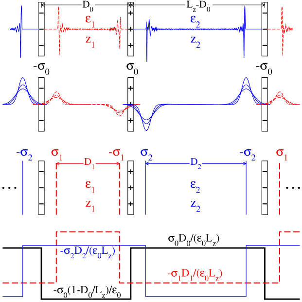
Figure 1: Periodic model of two liquid dielectrics with relative permittivities of $\varepsilon_{1}$ and $\varepsilon_{2}$ responding to contact charged walls and an applied constant electric field. Narrow columns in the upper, middle-upper and middle-lower panels refer to the fixed walls with surface charge densities of $\pm\sigma_{0}$ and their periodic images. The fixed walls are located in the $xy$ plane. The applied (app) external electric field (not shown) is along the $z$ direction with a magnitude of $E_{\rm app}$. $z_{1}$ and $z_{2}$ denote $z$ positions of the two bulk regions respectively. Periodic mobile charge densities of the two liquids, $\rho^{q}_{1}(z)$ and $\rho^{q}_{2}(z)$ are depicted by red dash and blue thin solid lines respectively in the upper panel, along with the corresponding periodic smoothed charge densities, $\rho^{q,\lambda}_{1}(z)$ and $\rho^{q,\lambda}_{2}(z)$ with three values of $\lambda$ and the corresponding periodic interfaces of countercharges in the middle-upper and middle-lower panels respectively. The distances between a pair of oppositely charged interfaces of countercharges, $D_{1}$ and $D_{2}$ are nearly constant with respect to the change of the electric field, $E_{\rm app}$ or the fixed surface charge density, $\sigma_{0}$. This constancy is guaranteed in dilute systems and further demonstrated in Fig. 2 for an example of concentrated charges. The lower panel gives the periodic alternating electric field, $E^{\rm e3dtf}(z;[\rho^{q}])$ produced by the e3dtf potential for both fixed (black thick solid line, $\pm\sigma_{0}$) and mobile (red dash line, $\pm\sigma_{1}$ and blue thin solid lines, $\pm\sigma_{2}$) surface charge densities. See Eqs. 9 and 11. The area formed by any of the three electric fields and the $z$-axis (not shown) in any period of $L_{z}$ would be zero, indicating the compensating boundary condition of Eq. 10. By matching the difference between the two SPMF potentials, $\nu_{\rm sp0}(z)$ and $\nu^{\rm e3dtf}_{\rm sp}(z)$ defined in Eqs. 4 and 5, the acting electric fields on both liquids are corrected to reestablish agreement with the macroscopic definitions of $\varepsilon_{1}$ and $\varepsilon_{2}$, either of which could be $1$, $>1$ but finite, or $\infty$ referring to the vacuum, a polar solvent, or an electrolyte respectively.

On the other hand, a recent stimulating work by Zhang and Sprik (ZS) have shown that when the e3dtf method is used for charged insulator/electrolyte interfaces (confined for the vacuum insulator and extended for the material insulator) in the $xy$ plane, the electric double layers (EDL) formed at the solid-electrolyte interface are indeed not fully charge compensated because of the finite $L_{z}$ and hence the finite width of the insulator slab usedZhang and Sprik (2016). They have further applied the constant electric field methodsStengel et al. (2009) to derive a linear relation between the net EDL charge and the applied electric field for given $L_{z}$. Their linear equation agrees excellently with the simulation data for the vacuum insulator (confined), however only qualitatively capture the feature in the range of weak electric fields for the water insulator (extended).

The two previous workPan et al. (2017); Zhang and Sprik (2016) certainly call for a general treatment of the finite-size effect arising from $\nu^{\rm e3dtf}$ for extended systems of charged interfaces. It is difficult to develop such a treatment because rigorous handlings of electrostatics for an extended system under the periodic boundary condition (PBC) are not even conceptually available. In this paper, we overcome this problem by conjecturing that a symmetry-preserving mean-field (SPMF) conditionHu (2014b) must be satisfied by any accurate method to reestablish agreement with macroscopic continuum electrostatics. The e3dtf simulation of the response of coexisting dielectric fluids to charged walls and a constant electric field is then forced to match the SPMF condition by intuitively adding both inbound and outbound corrections to the effective acting electric fields. The inbound correction reduces to the previous mean-field relation for a confined systemPan et al. (2017) while the outbound correction successfully accounts for the nonlinear coupling between the two liquids.

In the next section, we derive mean-field equations correcting the response of the two dielectric fluids with relative permittivities of $\varepsilon_{1}$ and $\varepsilon_{2}$ shown in Fig. 1. When the mobile charge densities of the two liquids are approximated as pairs of surface charge densities, $\pm\sigma_{1}$ and $\pm\sigma_{2}$ separated by stationary distances $D_{1}$ and $D_{2}$ respectively, the mean-field equations reduce to simple analytic relations among $\sigma_{1}$, $\sigma_{2}$, $\varepsilon_{1}$, $\varepsilon_{2}$, $D_{1}$, and $D_{2}$ under arbitrary conditions of the setup lengths $L_{z}$ and $D_{0}$, the fixed surface charge density $\sigma_{0}$ and the external electric field $E_{\rm app}$. No new simulations are carried out to validate the mean-field theory in this work. Instead, we reinterpret the simulation results in the literature to undoubtedly demonstrate its predictions for three examples: (i) confined water, (ii) confined electrolyte and (iii) an extended system of coexisting water and electrolyte. The well-justified mean-field approximations further suggest proper handlings of electrostatics for simulations of charged interfaces. Although we focus on systems with perfect planar symmetry, we finally argue that the mean-field treatment of the finite-size effect is relevant for general biomolecular simulations.

II A mean-field theory correcting dielectric responses

Macroscopic continuum electrostatics states that a constant electric field in the $z$ direction polarizes a dielectric fluid exposed to a solid surface in the $xy$ plane such that the mobile charges of the fluid reorganize to form a nonuniform charge density $\rho^{q}(z)$, that produces an internal polarization field defined by integrating the Poisson’s equation

$$E_{p}(z;[\rho^{q}])=\frac{1}{\varepsilon_{0}}\int^{z}dz^{\prime}\,\rho^{q}(z^{\prime}),$$ (3)

where the integral takes a position at which $\rho^{q}$ vanishes (e.g. the location of the solid surface) as its lower bound. In the bulk region $z=z_{b}$ where $\rho^{q}(z_{b})$ vanishes again, $E_{p}(z_{b};[\rho^{q}])$ partially cancels the external acting electric field. The factor by which the overall intrinsic electric field in the bulk decreases relative to the acting electric field defines the relative permittivity (dielectric constant) of the material.

For the extended system of Fig. 1 where the two surfaces confining the dielectric material $\varepsilon_{1}$ are in contact with the other dielectric material $\varepsilon_{2}$, it is difficult to introduce a proper treatment of electrostatics such that both materials respond correctly to the apparent acting electric fields. The SPMF approach claims that one may keep some short-ranged component of the Coulomb potential $\nu_{0}({\mathbf{r}})$ unchanged but average its remaining slowly-varying long-ranged component in the $x$ and $y$ directions with preserved symmetry to achieve efficient and accurate simulations of structural, thermodynamic and even dynamic propertiesHu (2014b). Any accurate (acc) SPMF treatment, $\nu^{\rm acc}({\mathbf{r}})$ must therefore satisfy the SPMF condition

$$\nu_{\rm sp0}(z)\equiv\left<\nu^{\rm acc}({\mathbf{r}})\right>_{\rm sp}=\frac{1}{A}\iint dxdy\,\nu_{0}({\mathbf{r}})=\frac{-|z|}{2\varepsilon_{0}A},$$ (4)

where the integral is taken over the infinite area for $\nu_{0}({\mathbf{r}})$ or $A=L_{x}L_{y}$ for $\nu^{\rm acc}({\mathbf{r}})$. $\left<\,\right>_{\rm sp}$ defines the SPMF potential as the average over the degrees of freedom in the directions with preserved symmetry in generalHu (2014b); Yi et al. (2017b). We now conjecture that the SPMF condition serves as a guiding constrain in building any accurate treatment of electrostatics in a finite setup that is consistent with the above macroscopic description of the dielectric response. In practice, $\nu^{\rm e3dtf}({\mathbf{r}})$ is commonly used for the supercell modeling of the extended system. The corresponding SPMF potential reads

$$\nu^{\rm e3dtf}_{\rm sp}(z)\equiv\left<\nu^{\rm e3dtf}({\mathbf{r}})\right>_{\rm sp}=\frac{\tau^{\rm 3D}}{4\pi\varepsilon_{0}}+\frac{1}{\varepsilon_{0}V}\sum_{s\neq 0}\frac{e^{isz}}{s^{2}},$$ (5)

where $s=2\pi k_{z}/L_{z}$ with $k_{z}$ integers. $\nu_{\rm sp0}(z)$ and $\nu^{\rm e3dtf}_{\rm sp}(z)$ differ by a quadratic function for $z\in[-L_{z},L_{z}]$

$$\nu_{\rm sp1}(z)=\nu^{\rm e3dtf}_{\rm sp}(z)-\nu_{\rm sp0}(z)=z^{2}/(2\varepsilon_{0}V)+C,$$ (6)

where the constant $C=\tau^{\rm 3D}/(4\pi\varepsilon_{0})+L_{z}/(12\varepsilon_{0}A)$. They satisfy the Poisson’s equation defined with two different charge densities respectively, the unit surface charge density for the former

$$-\nabla^{2}\nu_{\rm sp0}(z)=\delta(z)/(\varepsilon_{0}A),$$ (7)

and the periodic unit surface charge density with a compensating uniform background for the latter

$$-\nabla^{2}\nu^{\rm e3dtf}_{\rm sp}(z)=-\frac{1}{\varepsilon_{0}V}+\frac{1}{\varepsilon_{0}A}\sum_{n=-\infty}^{\infty}\delta(z-nL_{z}),$$ (8)

where $\delta(z)$ is the Dirac delta function. According to the superposition principle, the e3dtf electric field for any planar charge density $\rho^{q}(z)$ is given by

$$E^{\rm e3dtf}(z;[\rho^{q}])\equiv-A\frac{d}{dz}\int_{0}^{L_{z}}dz^{\prime}\,\rho^{q}(z^{\prime})\nu^{\rm e3dtf}_{\rm sp}(z-z^{\prime}),$$ (9)

where the interval of the integration, $[0,L_{z}]$ could always be an arbitrary period of $L_{z}$. $E^{\rm e3dtf}(z;[\rho^{q}])$ alternates within any period and satisfies a compensating boundary condition

$$\int_{0}^{L_{z}}E^{\rm e3dtf}(z;[\rho^{q}])\equiv 0,$$ (10)

which essentially reflects the periodicity of $\nu^{\rm e3dtf}_{\rm sp}(z)$. For the specific fixed charge density $\rho^{q}_{f}(z)$ represented by the two charged walls separated by $D_{0}$ in Fig. 1, $E^{\rm e3dtf}(z;[\rho^{q}_{f}])$ gives exactly two constant electric fields for the regions inside and outside the walls respectively

$$E^{\rm e3dtf}(z_{j};[\rho^{q}_{f}])=\left\{\begin{array}[]{lr}-\sigma_{0}(L_{z}-D_{0})/(\varepsilon_{0}L_{z})&j=1\\ \sigma_{0}D_{0}/(\varepsilon_{0}L_{z})&j=2\end{array}\right.$$ (11)

where $z_{j}$ ($j=1$ or $2$) denotes any $z$ position in the bulk of the material $j$. In contrast, the usual electric field for the two charged walls must be $-\sigma_{0}/\varepsilon_{0}$ inside and $0$ outside. $E^{\rm e3dtf}(z;[\rho^{q}_{f}])$ therefore involves a finite-size correction, $\sigma_{0}D_{0}/(\varepsilon_{0}L_{z})$ for both regions.

There exits an intuitive understanding of the finite-size effect caused by the nonuniform mobile charge densities of the two materials, $\rho^{q}_{1}(z)$ and $\rho^{q}_{2}(z)$ as well. Noting that $\nu_{\rm sp1}(z)$ is slowly varying relative to $\nu_{\rm sp0}(z)$ and short-ranged parts of other van der Waals interactions, the instantaneous electric field from $\nu_{\rm sp1}(z)$ thus fluctuates weakly configuration by configuration in crowded environmentHu (2014b) and can be safely approximated by its equilibrium average

$$E_{c}(z;[\rho^{q}])\simeq-A\frac{d}{dz}\int dz^{\prime}\,\rho^{q}(z^{\prime})\nu_{\rm sp1}(z-z^{\prime}),$$ (12)

where the range of the integration, if not stated, is always the whole continuous region defining $\rho^{q}(z)$. $z$ spans over the regions of the two materials and $z-z^{\prime}\in[-L_{z},L_{z}]$ necessarily. The usual minimum image convention resulting in $|z-z^{\prime}|^{\rm min}\leqslant L_{z}/2$ is therefore not applied here ! As will be discussed later, this violation of PBC has an important consequence on the proper treatments of electrostatics. Anyway, the simulation done with $\nu^{\rm e3dtf}({\mathbf{r}})$ is now effectively mapped into the simulation done artificially with $\nu_{0}({\mathbf{r}})$ subject to an additional electric field $E_{c}(z;[\rho^{q}])$, that accounts for the average effect arising from their difference. This static limit of the SPMF approximation resembles the local molecular field (LMF) approximation developed by Weeks and co-workers Weeks (2002); Rodgers and Weeks (2008); Hu and Weeks (2010); Remsing et al. (2016). However, the present application differs from that of LMF theory in three aspects. (i) While LMF theory connects a full system with a long-ranged interaction to a simpler reference system with a short-ranged interaction, both $\nu^{\rm e3dtf}({\mathbf{r}})$ and $\nu_{0}({\mathbf{r}})$ are long-ranged. (ii) When the relative distance increases, the usual long-ranged component in LMF theory tends to $0$ but $\nu_{\rm sp1}(z)$ increases all the way up to $z=L_{z}$. (iii) LMF theory often solves iteratively the spatially varying effective potential, this static approximation yields instead a constant electric field proportional to the total dipole moment of the material

$$E_{c}(z;[\rho^{q}])\equiv E_{c}([\rho^{q}])=\frac{1}{\varepsilon_{0}L_{z}}\int dz^{\prime}\,z^{\prime}\rho^{q}(z^{\prime}),$$ (13)

when the electroneutrality condition, $\int dz\,\rho^{q}(z)=0$ is applied. In total, each dielectric material $j$ ($j=1$ or $2$) responds effectively (eff) to a sum of four constant electric fields

$$E^{\rm eff}_{j}=E_{\rm app}+E^{\rm e3dtf}(z_{j};[\rho^{q}_{f}])+E_{c}([\rho^{q}_{1}+\rho^{q}_{2}]),$$ (14)

where the last term must consist of an inbound correction (c), $E_{c}([\rho^{q}_{j}])$ arising from the material $j$ itself and an outbound correction arising from the other material. In addition, the outbound correction $E_{c}([\rho^{q}_{1/2}])$ reduces completely to $E^{\rm e3dtf}(z_{2/1};[\rho^{q}_{1/2}])$ and thus fully describes the coupling between the two materials, which is consistent with the fact that the usual electric field due to $\nu_{\rm sp0}(z)$ always vanishes outside a neutral material.

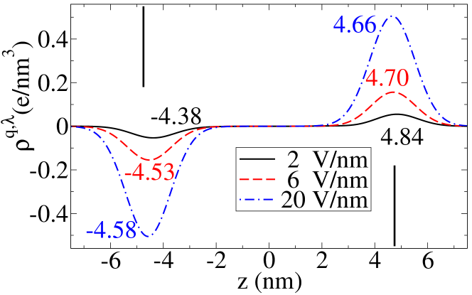
Figure 2: Smoothed charge densities $\rho^{q,\lambda}(z)$ of confined SPC/E water under the three acting electric fields of $2$ (solid line), $6$ (red dash line) and $20$ (blue dot dash line) volts/nm simulated previouslyHu (2014b). The $z$ positions of the peaks and troughs are indicated by the nearby numbers. The two straight lines refer to the walls at $z=\pm 4.75$. As a consequence of the very strong oscillations of the unsmoothed charge density under a weak electric field, one peak at $4.84\,{\rm nm}$ goes beyond the position of the wall. $\rho^{q,\lambda}(z)$ shifts in the $z$ direction with an almost constant distance ($\simeq 9.22$ nm) between the two branches. $\lambda=1.2\,{\rm nm}$ and similar observations are made for other values of $\lambda$. The walls are shifted outwards by $2.5\,{\rm nm}$ each for clarity.

The dielectric response of each material $\varepsilon_{j}$ corrected by the finite $L_{z}$ associated with the use of the e3dtf method follows

$$E^{\rm eff}_{j}+E_{p}(z_{j};[\rho^{q}_{j}])=E^{\rm eff}_{j}/\varepsilon_{j}\quad{\rm for}\quad j=1\,\,{\rm or}\,\,2,$$ (15)

which however is difficult to solve because $\rho^{q}_{j}(z)$ involved in Eqs. 3 and 13 oscillates strongly on the scale of intermolecular distances. In fact, both equations can be re-expressed exactly as functionals of an auxiliary smoothed charge density, $\rho^{q,\lambda}(z)$: $E_{c}([\rho^{q}])=E_{c}([\rho^{q,\lambda}])$ and $E_{p}(z_{b},[\rho^{q}])=E_{p}(z_{b},[\rho^{q,\lambda}])$, where $\rho^{q,\lambda}(z)$ may be defined by convoluting $\rho^{q}(z)$ with a normalized Gaussian function with width $\lambda$ that exceeds a typical intermolecular distance of subnanometer

$$\rho^{q,\lambda}(z)=\int dz^{\prime}\,\rho^{q}(z^{\prime})\frac{1}{\sqrt{\pi}\lambda}e^{-|z-z^{\prime}|^{2}/\lambda^{2}}.$$ (16)

Furthermore, when denoting the total surface charge density in the left side as $\sigma_{j}$, shown in Fig 1, and subsequently the surface charge dipole moment as $-\sigma_{j}D_{j}$, $E_{p}(z_{j};[\rho^{q}_{j}])=\sigma_{j}/\varepsilon_{0}$ and $E_{c}([\rho^{q}_{j}])=-\sigma_{j}D_{j}/(\varepsilon_{0}L_{z})$. Given that the length of the material $j$ in the $z$ direction is sufficiently large ($>\lambda$) that the two interfaces of the same material are well separated by the bulk, $D_{j}$ must stand for the distance between the two oppositely charged branches of any properly chosen $\rho^{q,\lambda}_{j}(z)$. At the limit of dilute ions for which the linearized Poisson-Boltzmann theory applies, the charge density is proportional to $e^{-k_{D}z}$ with $k_{D}$ the inverse Debye lengthHansen and McDonald (2013) and $D_{j}$ must be exactly independent of the acting electric field. As an example of concentrated charges in a dense fluid, $\rho^{q,\lambda}(z)$ of confined SPC/E waterHu (2014b) shown in Fig. 2 suggests that $D_{j}$ is still nearly a constant although the whole $\rho^{q,\lambda}(z)$ slips upon the change of the acting electric field. Any liquid-solid interface may arguably be characterized by a stationary distance resulting from a balance between competing van der Waals and Coulomb forces.

Given the algebraic expressions of $E_{p}(z_{j};[\rho^{q}_{j}])$ and $E_{c}([\rho^{q}_{j}])$, Eq. 15 turns into two coupled relations between the input parameters $E_{\rm app}$, $L_{z}$, $D_{0}$, and $\sigma_{0}$, and the unknown surface charge densities $\sigma_{1}$ and $\sigma_{2}$ for the given characteristics of $\varepsilon_{1}$, $\varepsilon_{2}$, $D_{1}$ and $D_{2}$. It is crucial that $D_{j}$ depends on neither $\sigma_{0}$ nor $E_{\rm app}$. Otherwise, Eq. 15 would not be analytically solvable. Such simplification reflects essentially that the oscillations of $\rho^{q}_{j}(z)$ on the small intermolecular length scale hardly influence the integrated properties on the much larger scale.

III Applications: charged polar and electrolytic interfaces

We now examine the validity of the corrected dielectric response described by Eq. 15 for three charged interfaces of polar and/or electrolytic systems. In the first example of confined SPC/E waterBerendsen et al. (1987) between the two planar wallsLee et al. (1984) investigated previously by usPan et al. (2017), $E_{\rm app}=2$ volts/nm, $\sigma_{0}=0$, $\varepsilon_{1}\simeq 78$ for SPC/E water under weak electric fieldsPan et al. (2017), and $\varepsilon_{2}=1$ for the vacuum. Therefore, Eq. 15 only involves the inbound correction and thus reduces to Eq.(83) in ref.Pan et al. (2017), which was derived alternatively by analyzing the difference between the e3dtf method and the Ewald2D method. However, the present derivation based on the SPMF constraint is more solid and generally applicable without addressing any specific treatment of electrostatics. It has been verified that the simulated $\rho^{q}_{1}(z)$ using e3dtf with four different setups of $L_{z}$ indeed responds to the corresponding effective acting electric field, $E_{c}[\rho^{q}_{1}]+E_{\rm app}$. Moreover, without knowing $\rho^{q}_{1}(z)$, the inbound correction relative to the applied electric field, $E_{c}([\rho^{q}_{1}])/E_{\rm app}$ is predicted to be

$$E_{c}([\rho^{q}_{1}])/E_{\rm app}=(1-1/\varepsilon_{1})/(L_{z}/D_{1}-1+1/\varepsilon_{1}),$$ (17)

which is formally identical to Eq.(89) of ref.Pan et al. (2017) except that it becomes meaningful to assign an accurate value for $D_{1}$ now. Indeed, Fig. 3 shows that this analytic relation agrees excellently with the simulation results when taking $D_{1}=4.22\,{\rm nm}$ rather than approximating $D_{1}\simeq 4\,{\rm nm}$ as in ref. Pan et al. (2017).

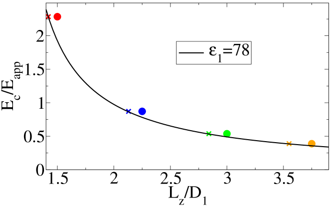
Figure 3: Relative corrections to the applied electric field, $E_{\rm c}/E_{\rm app}$ plotted as a function of $L_{z}/D_{1}$. The solid line corresponds to Eq. 17 with $\varepsilon_{1}=78$. Symbols indicate simulation results for $L_{z}=6$, $9$, $12$, and $15$ nm at $D_{1}=4.22\,{\rm nm}$ (crosses) or $D_{1}=4\,{\rm nm}$ (filled circles taken from Fig.8 of refPan et al. (2017)).

The importance of determining precisely the value of $D_{j}$ is further demonstrated by applications of Eq. 15 to two other examples of insulator/electrolyte interfaces. In the two EDL systems investigated previously by ZS, $\varepsilon_{1}=\infty$ for the electrolyte. Eliminating $\sigma_{2}$ from the coupled equations of corrected dielectric response yields analytically

$$(\sigma_{1}-\sigma_{0})(L_{z}-D_{1}-D_{2}+D_{2}/\varepsilon_{2})=\\ \varepsilon_{0}(-E_{\rm app}L_{z})-\sigma_{0}(D_{0}-D_{1}),$$ (18)

and $E_{2}^{\rm eff}=(\sigma_{0}-\sigma_{1})/\varepsilon_{0}$. For the vacuum insulator, $\varepsilon_{2}=1$ as in the previous example. The slope of the linear relation between the net EDL charge, $(\sigma_{1}-\sigma_{0})A$ and the applied voltage, $-E_{\rm app}L_{z}$ is predicted to be $A\varepsilon_{0}/(L_{z}-D_{1})$ with $D_{1}=3.724$ nm matching the unified $x$-intercept of $8.9$ volts found by ZSZhang and Sprik (2016). This linear relation is confirmed by the simulation results shown in Fig. 4(a) for three setups of $L_{z}$. Alternatively, ZS have introduced a Stern-type model to interpret successfully their findings for this vacuum insulator, which inspired us to develop the present mean-field approach to elucidate the underlying microscopic mechanism.

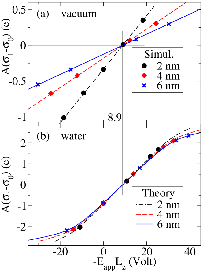
Figure 4: The net EDL charge as a function of the external voltage for the vacuum (a) and water (b) insulators. Simulation data are taken from Fig. 6 and Fig. 8 of ref Zhang and Sprik (2016) where $D_{0}=4.124\,{\rm nm}$, $L_{x}=L_{y}=1.275\,{\rm nm}$, $A\sigma_{0}=2{\rm e}$, and $L_{z}$ equals $D_{0}$ plus the thickness of the insulator slab: $2$ (circles), $4$ (diamonds), or $6$ (crosses) nm. Analytic results are given by Eq. 18 at $D_{0}-D_{1}=0.4\,{\rm nm}$ and $L_{z}-D_{0}-D_{2}=0.445\,{\rm nm}$ with a reasonable expression, Eq. 19 for the field-dependent $\varepsilon_{2}$notedielectric . The straight line indicates the invariant zero net charge point $(8.9{\rm V},0{\rm e})$ for any insulator.

Indeed, such an attempt leads to even more satisfactory analysis of e3dtf simulation for any material insulator with $\varepsilon_{2}=\varepsilon_{2}(E_{2}^{\rm eff})$ depending on the acting electric field $E_{2}^{\rm eff}$ in general. For the SPC/E water insulator, one may use the expression derived by Booth for the field-dependent relative permittivityBooth (1951); notedielectric

$$\varepsilon_{2}=n^{2}+\frac{7\rho_{b}(n^{2}+2)\mu}{3\varepsilon_{0}\sqrt{73}E_{\rm in}}L\left[\frac{\sqrt{73}\mu(n^{2}+2)E_{\rm in}}{6k_{b}T}\right],$$ (19)

where $E_{\rm in}=|E_{2}^{\rm eff}|/\varepsilon_{2}=|\sigma_{0}-\sigma_{1}|/(\varepsilon_{0}\varepsilon_{2})$ is the absolute value of the overall intrinsic electric field exerted on the bulk. $L(x)={\rm coth}(x)-1/x$ is the Langevin function. $\mu=0.04894{\rm e\cdot nm}$ and $\rho_{b}=33.46/{\rm nm}^{3}$ are the dipole moment and the number density at the temperature $T=298{\rm K}$ respectively. $k_{b}$ is the Boltzmann constant. The refractive index is adjusted slightly, $n=1.113$ such that the dielectric constant at a weak electric field $\simeq 78$. Because of the coupling between the electrolyte and the material insulator, Eqs. 18 and 19 suggest that the relation between the net EDL charge and the applied voltage is nonlinear and symmetric with respect to the point of the $x$-intercept, $(8.9{\rm V},0{\rm e})$, where the slope reaches the maximum, $A\varepsilon_{0}/(L_{z}-D_{1}-D_{2}+D_{2}/78)$ and then decreases monotonically down to that of the vacuum insulator, $A\varepsilon_{0}/(L_{z}-D_{1})$ as the absolute value of the net EDL charge increases. Fig. 4(b) shows that this nonlinear relation agrees surprisingly well with the simulation results for the three setups of $L_{z}$ given that $L_{z}-D_{0}-D_{2}=0.445\,{\rm nm}$ is a constant. More importantly, Eq. 18 predicts that the unified $x$-intercept representing the state of complete charge compensation, is invariant with respect to solvent permittivities, which is undoubtedly confirmed by Fig. 4 for the two examples of insulator/electrolyte interfaces.

IV Discussion: proper treatments for charged interfaces

The present extended system may correspond to a very thin material $1$ ($D_{0}\sim$ nm) confined between the two charged walls, both exposed to the same macroscopic material $2$ from the other sides. In the $x$ and $y$ directions where the charges are uniformly distributed, the usual PBCs are safely applied. This section discusses three boundary conditions: non-, full-, and semi-PBCs in the $z$ direction.

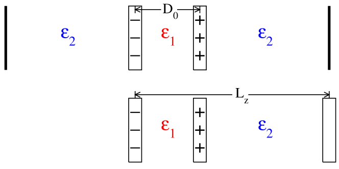
Figure 5: Setups of non-PBC (upper) and semi-PBC (lower) in the $z$-direction in contrast with the full-PBC in Fig. 1. Under the semi-PBC, the minimum image convention due to PBC is only imposed on short-ranged interactions; charges appear instead continuously with no images when evaluating $z_{ij}$ of each pair for the long-ranged electrostatic interaction.

A natural way to mimic the realistic system is the non-PBC setup in Fig. 5, under which two hard walls are introduced to turn the extended system into a much larger confined system. Accurate algorithms for electrostatics in slab geometry include the Ewald2D sum methodsParry (1975); Heyes et al. (1977); de Leeuw and Perram (1979); Pan and Hu (2014, 2015), the Ewald3D sum with the planar infinite boundary term methodsSmith (1981); Yeh and Berkowitz (1999); Hu (2014a); dos Santos et al. (2016); Yi et al. (2017a), and othersHautman and Klein (1992); Boda et al. (1998); Arnold and Holm (2002); Hu (2014b), which all satisfy exactly the SPMF condition in Eq. 4. Recent techniques developed for efficient simulations of bulk systemsWang et al. (2016); Vatamanu et al. (2018) can also be used for confined systems after adding an extra $z$-dependent term to make the algorithms match the SPMF condition as previously doneHu (2014b).

An advantage of using the full-PBC in Fig. 1 is to minimize the edge effect in a relatively smaller unit cell. The present mean-field theory immediately suggests that the e3dtf method still works for simulating desired responses of both materials when two auxiliary constant electric fields are applied on the materials to offset the unwanted components of $E_{1}^{\rm eff}$ and $E_{2}^{\rm eff}$ respectively. The auxiliary electric fields depend on the setup and the intrinsic properties of $\varepsilon_{1}$, $\varepsilon_{2}$, $D_{1}$ and $D_{2}$, which can all be predetermined from trial simulations, as evidenced by the perfect fittings in Figs 3 and 4.

Instead of applying statically predetermined auxiliary fields, it is convenient to offset the unwanted finite-size effect by adding instantaneously $-q_{i}q_{j}z_{ij}^{2}/(2\epsilon_{0}V)$, the negative of Eq. 6, to each pair of charges. This instantaneous correction is formally identical to the planar infinite boundary termSmith (1981); Hu (2014a) but should be interpreted in the setup of semi-PBC in Fig. 5, where $z_{ij}\in[-L_{z},L_{z}]$ rather than $z_{ij}^{\rm min}\in[-L_{z}/2,L_{z}/2]$ due to the PBC. Because $\nu^{\rm e3dtf}(z_{ij})=\nu^{\rm e3dtf}(z_{ij}^{\rm min})$ remains unchanged, the semi-PBC corresponds to applying PBC only for short-ranged interactions and therefore interprets appropriately the SPMF condition. Besides, it is more accurate in principle than the above full-PBC scheme because the involved SPMF approximation is always superior to its static limitHu (2014b); Yi et al. (2017b). The aforementioned other techniques for confined systems are applicable as well provided that $z_{ij}$ involved in the techniques is correctly evaluated under the same semi-PBC. To our knowledge, the semi-PBC scheme has not been implemented for any extended system before but has both advantages of using a smaller unit cell and carrying out no trial simulations.

V Conclusions and Outlook

We have demonstrated that the SPMF condition serves as a necessary constrain for any accurate handling of electrostatics in systems of charged interfaces. The mean-field equation accounting for the difference between the usual e3dtf method and the SPMF condition is useful for providing transparent analysis of the associated finite-size effect. Proper analysis of e3dtf simulations of any extended polar or charged system is expected to validate undoubtedly the analytic predictions from the mean-field equation. In addition, the mean-field theory suggests an efficient and accurate semi-PBC scheme that reconciles directly the simulated charge reorganization with the macroscopic dielectric response. We expect this approach to be of significant importance to the study of large interfaces of materials and biological membranes with their surface corrugations on a scale where the long-ranged electrostatics varies sufficiently slowly.

Although the present theory is based on classical point charge models, we are optimistic that the mean-field idea can be extended to both quantum mechanical calculationsCheng et al. (2014) and sophisticated models involving electric multipole potentialsLi et al. (2016). As such, we view the present work as a demonstration of the ability of the SPMF approach to treat accurately and to understand analytically electrostatics in various complex molecular interfaces.

VI Acknowledgement

This work was supported by the NSFC Grant (No.21522304) and the Program for JLU Science and Technology Innovative Research Team (JLUSTIRT).

References

- Yi et al. (2015) Shasha Yi, Cong Pan, and Zhonghan Hu, “Accurate treatments of electrostatics for computer simulations of biological systems: A brief survey of developments and existing problems,” Chin. Phys. B 24, 120201 (2015).
- Steinbach and Brooks (1994) Peter J. Steinbach and Bernard R. Brooks, “New spherical-cutoff methods for long-range forces in macromolecular simulation,” J. Comput. Chem. 15, 667–683 (1994).
- Feller et al. (1996) Scott E. Feller, Richard W. Pastor, Atipat Rojnuckarin, Stephen Bogusz, and Bernard R. Brooks, “Effect of electrostatic force truncation on interfacial and transport properties of water,” J. Phys. Chem. 100, 17011–17020 (1996).
- Yonetani (2005) Yoshiteru Yonetani, “A severe artifact in simulation of liquid water using a long cut-off length: Appearance of a strange layer structure,” Chem. Phys. Letters 406, 49 – 53 (2005).
- Ewald (1921) P. P. Ewald, “Evaluation of optical and electrostaic lattice potentials,” Annalen der Physik, Leipzig 369, 253–287 (1921).
- de Leeuw et al. (1980) S. W. de Leeuw, J. W. Perram, and E. R. Smith, “Simulation of electrostatic systems in periodic boundary conditions. i. lattice sums and dielectric constants,” Proc. R. Soc. London, Ser. A Math. Phys. Sci. 373, 27–56 (1980).
- Cisneros et al. (2014) G. Andres Cisneros, Mikko Karttunen, Pengyu Ren, and Celeste Sagui, “Classical electrostatics for biomolecular simulations,” Chemical Reviews 114, 779–814 (2014).
- Frenkel and Smit (2002) Daan Frenkel and Berend Smit, Understanding Molecular Simulation: From Algorithms to Applications, 2nd ed. (Academic Press, Inc., San Diego, 2002).
- Hu (2014a) Zhonghan Hu, “Infinite boundary terms of ewald sums and pairwise interactions for electrostatics in bulk and at interfaces,” J. Chem. Theory Comput. 10, 5254–5264 (2014a).
- Yi et al. (2017a) Shasha Yi, Cong Pan, and Zhonghan Hu, “Note: A pairwise form of the ewald sum for non-neutral systems,” J. Chem. Phys. 147, 126101 (2017a).
- (11) While the usual pairwise form (e.g. eq.(3) of ref.Yi et al. (2017a)) with a finite screening factor has to be used for an efficient computation, this concise and convenient expression Eq. 2 corresponding to yields inevitably rigorous results for operations of derivative and integration, as in later Eqs. 5 and 9.
- Pan et al. (2017) Cong Pan, Shasha Yi, and Zhonghan Hu, “The effect of electrostatic boundaries in molecular simulations: symmetry matters,” Phys. Chem. Chem. Phys. 19, 4861 (2017).
- Parry (1975) D.E. Parry, “The electrostatic potential in the surface region of an ionic crystal,” Surf. Sci. 49, 433 – 440 (1975).
- Heyes et al. (1977) D. M. Heyes, M. Barber, and J. H. R. Clarke, “Molecular dynamics computer simulation of surface properties of crystalline potassium chloride,” J. Chem. Soc., Faraday Trans. II: Mol. Chem. Phys. 73, 1485–1496 (1977).
- de Leeuw and Perram (1979) S. W. de Leeuw and J. W. Perram, “Electrostatic lattice sums for semi-infinite lattices,” Mol. Phys. 37, 1313–1322 (1979).
- Pan and Hu (2014) Cong Pan and Zhonghan Hu, “Rigorous error bounds for ewald summation of electrostatics at planar interfaces,” J. Chem. Theory Comput. 10, 534–542 (2014).
- Pan and Hu (2015) Cong Pan and Zhonghan Hu, “Optimized ewald sum for electrostatics in molecular self-assembly systems at interfaces,” Sci. China Chem. 58, 1044–1050 (2015).
- Smith (1981) E. R. Smith, “Electrostatic energy in ionic crystals,” Proc. R. Soc. London, Ser. A Math. Phys. Sci. 375, 475 (1981).
- Zhang and Sprik (2016) Chao Zhang and Michiel Sprik, “Finite field methods for the supercell modeling of charged insulator/electrolyte interfaces,” Phys. Rev. B 94, 245309 (2016).
- Stengel et al. (2009) Massimiliano Stengel, Nicola A. Spaldin, and David Vanderbilt, “Electric displacement as the fundamental variable in electronic-structure calculations,” Nat. Phys. 5, 304–308 (2009).
- Hu (2014b) Zhonghan Hu, “Symmetry-preserving mean field theory for electrostatics at interfaces,” Chem. Commun. 50, 14397–14400 (2014b).
- Yi et al. (2017b) Shasha Yi, Cong Pan, Liming Hu, and Zhonghan Hu, “On the connections and differences among three mean-field approximations: a stringent test,” Phys. Chem. Chem. Phys. 19, 18514–18518 (2017b).
- Weeks (2002) John D. Weeks, “Connecting local structure to interface formation: A molecular scale van der waals theory of nonuniform liquids,” Annu. Rev. Phys. Chem. 53, 533–562 (2002).
- Rodgers and Weeks (2008) Jocelyn M. Rodgers and John D. Weeks, “Interplay of local hydrogen-bonding and long-ranged dipolar forces in simulations of confined water,” Proc. Natl. Acad. Sci. USA 105, 19136–19141 (2008).
- Hu and Weeks (2010) Zhonghan Hu and John D. Weeks, “Efficient solutions of self-consistent mean field equations for dewetting and electrostatics in nonuniform liquids,” Phys. Rev. Lett. 105, 140602 (2010).
- Remsing et al. (2016) R. C. Remsing, S. Liu, and J. D. Weeks, “Long-ranged contributions to solvation free energies from theory and short-ranged models,” Proc. Natl. Acad. Sci. USA 117, 2819–2826 (2016).
- Hansen and McDonald (2013) J. P. Hansen and I. R. McDonald, Theory of simple liquids with applications to soft matter, 4th ed. (Academic Press, Inc., Amsterdam, 2013).
- Berendsen et al. (1987) H. J. C. Berendsen, J. R. Grigera, and T. P. Straatsma, “The missing term in effective pair potentials,” J. Phys. Chem. 91, 6269–6271 (1987).
- Lee et al. (1984) C. Y. Lee, J. Andrew McCammon, and P. J. Rossky, “The structure of liquid water at an extended hydrophobic surface,” J. Chem. Phys. 80, 4448–4455 (1984).
- (30) In the present case, is still quite large at the moderately strong acting electric fields. , thus contributes little to Eq. 18 such that becomes insensitive to a detailed expression of the field-dependent dielectric constant, like Eq. 19, which was derived originally for realistic water but employed here for a classic SPC/E model of water. It is otherwise necessary to use an accurate expression of for the modeled fluid when approaches under very strong acting electric fields.
- Booth (1951) F. Booth, “The dielectric constant of water and the saturation effect,” J. Chem. Phys. 19, 391–394 (1951).
- Yeh and Berkowitz (1999) In-Chul Yeh and Max L. Berkowitz, “Ewald summation for systems with slab geometry,” J. Chem. Phys. 111, 3155–3162 (1999).
- dos Santos et al. (2016) Alexandre P. dos Santos, Matheus Girotto, and Yan Levin, “Simulations of coulomb systems with slab geometry using an efficient 3d ewald summation method,” J. Chem. Phys. 144, 144103 (2016).
- Hautman and Klein (1992) J. Hautman and M.L. Klein, “An ewald summation method for planar surfaces and interfaces,” Mol. Phys. 75, 379–395 (1992).
- Boda et al. (1998) Dezs Boda, Kwong-Yu Chan, and Douglas Henderson, “Monte carlo simulation of an ion-dipole mixture as a model of an electrical double layer,” J. Chem. Phys. 109, 7362–7371 (1998).
- Arnold and Holm (2002) Axel Arnold and Christian Holm, “Mmm2d: A fast and accurate summation method for electrostatic interactions in 2d slab geometries,” Comput. Phys. Commun. 148, 327 – 348 (2002).
- Wang et al. (2016) Han Wang, Haruki Nakamura, and Ikuo Fukuda, “A critical appraisal of the zero-multipole method: Structural, thermodynamic, dielectric, and dynamical properties of a water system,” J. Chem. Phys. 144, 114503 (2016).
- Vatamanu et al. (2018) Jenel Vatamanu, Oleg Borodin, and Dmitry Bedrov, “Application of screening functions as cutoff-based alternatives to ewald summation in molecular dynamics simulations using polarizable force fields,” J. Chem. Theory Comput. 14, 768–783 (2018).
- Cheng et al. (2014) Jun Cheng, Xiandong Liu, John A. Kattirtzi, Joost VandeVondele, and Michiel Sprik, “Aligning electronic and protonic energy levels of proton-coupled electron transfer in water oxidation on aqueous tio2,” Angew. Chem. Int. Ed. 53, 12046–12050 (2014).
- Li et al. (2016) Guohui Li, Hujun Shen, Dinglin Zhang, Yan Li, and Honglei Wang, “Coarse-grained modeling of nucleic acids using anisotropic gay-berne and electric multipole potentials,” J. Chem. Theory Comput. 12, 676–693 (2016).