Rectification in Spin-Orbit Materials Using Low Energy Barrier Magnets

Abstract

The coupling of spin-orbit materials to high energy barrier ($\sim$40-60 $k_{B}T$) nano-magnets has attracted growing interest for exciting new physics and various spintronic applications. We predict that a coupling between the spin-momentum locking (SML) observed in spin-orbit materials and low-energy barrier magnets (LBM) should exhibit a unique multi-terminal rectification for arbitrarily small amplitude channel currents. The basic idea is to measure the charge current induced spin accumulation in the SML channel in the form of a magnetization dependent voltage using an LBM, either with an in-plane or perpendicular anisotropy (IMA or PMA). The LBM feels an instantaneous spin-orbit torque due to the accumulated spins in the channel which causes the average magnetization to follow the current, leading to the non-linear rectification. We discuss the frequency band of this multi-terminal rectification which can be understood in terms of the angular momentum conservation in the LBM. For a fixed spin-current from the SML channel, the frequency band is same for LBMs with IMA and PMA, as long as they have the same total magnetic moment in a given volume. The proposed all-metallic structure could find application as highly sensitive passive rf detectors and as energy harvesters from weak ambient sources where standard technologies may not operate.

I Introduction

The interplay between spin-orbit materials and nano-magnetism has attracted much attention for interesting phenomena e.g. spin-orbit torque switching Liu et al. (2012a, b), probing the spin-momentum locking Li et al. (2014); Hus et al. (2017); Liu et al. (2015); Dankert et al. (2015); Pham et al. (2016); Lee et al. (2018), spin amplification Habib et al. (2015), spin battery Tian et al. (2017), skyrmion dynamics Woo et al. (2017); Yu et al. (2016), among other examples. In this paper, we predict that the spin-momentum locking (SML) observed in spin-orbit materials when coupled to a nano-magnet with low-energy barrier, will rectify the channel current in the form of a voltage in a multi-terminal structure. We start our arguments with the spin-potentiometric measurements well-established in diverse classes of spin-orbit materials (see, for example, Li et al. (2014); Hus et al. (2017); Liu et al. (2015); Dankert et al. (2015); Pham et al. (2016); Lee et al. (2018)) where a high-energy-barrier stable ferromagnet (FM) is used to measure the charge current induced spin potential in the SML channel. We show that such spin-potential measurement on a metallic SML channel using a low-energy barrier magnet (LBM) will result in a rectified voltage, even for arbitrarily small channel current.

The discussions on the multi-terminal rectification is limited in the linear response regime of transport in the SML channel and the non-linearity occurs due to the spin-orbit torque (SOT) driven magnetization dynamics of the LBM. We further show that the multi-terminal rectification is limited by a characteristic frequency of the LBM that can be understood in terms of angular momentum conservation between the spins injected from spin-orbit materials and the spins absorbed by the LBM. We argue that, for a fixed spin-current from the SML channel, the characteristic frequency is the same for LBMs with in-plane and perpendicular magnetic anisotropies (IMA and PMA), as long as they have the same total magnetic moment in a given volume.

We analyze the rectification in the proposed all-metallic structure (see Fig. 1(a)) considering both IMA and PMA LBMs and provide simple models to understand the underlying mechanisms of (i) the spin-orbit torque (SOT) induced magnetization pinning and (ii) the frequency band of the rectification. We compare the simple models with detailed numerical simulations using an experimentally benchmarked multi-physics framework Camsari et al. (2015). The simulations are carried out using a transmission line model for the SML channel Sayed et al. (2018) and a stochastic Landau-Lifshitz-Gilbert (s-LLG) model for LBM Camsari et al. (2017), considering thermal noise within the magnet. We consider the spin-polarization axis to be in-plane of the SML channel and orthogonal to the current flow direction. Hence, in the present discussion, pinning for a IMA or a PMA magnet occurs along the easy-axis or hard-axis, respectively.

We argue that such wideband rectification in an all-metallic structure (Fig. 1(a)) could be used for ‘passive’ radio frequency (rf) detection. Recently, Magnetic Tunnel Junction (MTJ) diodes with stable magnet as free layer and under an external dc current bias have demonstrated orders of magnitude higher sensitivity compared to the state-of-the-art Schottky diodes Miwa et al. (2013); Fang et al. (2016); Zhang et al. (2018). However, the reported no-bias sensitivity is lower or comparable to that of semiconductor diodes. The low-barrier nature of the magnet in the proposed structure should exhibit no-bias sensitivity as high as those observed using state-of-the-art technologies under external biases Miwa et al. (2013); Fang et al. (2016); Zhang et al. (2018). Furthermore, we discuss the possibility to harvest energy from weak ambient sources where standard technologies may not operate.

The paper is organized as follows. In Section II, we establish the concept of the multi-terminal rectification in the SML channel using LBM, starting from the well-established spin-potentiometric measurements typically done with high-energy-barrier stable magnets. In Section III, we discuss the frequency bandwidth of the rectification and provide a simple model that applies to LBMs with both IMA and PMA. We argue using detailed simulaiton results that such bandwidth arises due to the principles of angular momentum conservation between the spins injected from the SML channel and the spins absorbed by the LBM. In Section IV, we discuss possible applications of the proposed all-metallic structure in ‘passive’ rf detection and energy harvesting. We argue that the no-bias sensitivity of the proposed rectifier can be as high as those observed in state-of-the-art technologies under external bias. Finally, in Section V, we end with a brief conclusion.

II Multi-Terminal Rectification

We start our arguments with the well-established spin-potentiometric measurements Li et al. (2014); Hus et al. (2017); Liu et al. (2015); Dankert et al. (2015); Pham et al. (2016); Lee et al. (2018) where the charge current induced spin potential in the SML channel is measured in the form of a magnetization dependent voltage using a stable ferromagnet (FM). The voltage at the FM with respect to a reference normal metal (NM) contact, placed at the same position along the current path as the FM (see Fig. 1(a)), is given by Hong et al. (2012); Sayed et al. (2017)

$${V_{34}\left(\vec{m}\right)}={\left(\hat{s}\cdot\vec{m}\right)}\,\dfrac{{\alpha\xi{p_{0}}{p_{f}}R_{B}}}{{2}}{I_{12}},$$ (1)

which shows opposite signs for the two magnetic states of the FM under a fixed channel current $I_{12}$ flowing along $\hat{n}$-direction (see Fig. 1(a)). Here $\hat{s}$ is the spin polarization axis in the SML channel defined by $\hat{y}\times\hat{n}$ with $\hat{y}$ being the out-of-plane direction Sayed et al. (2018), $\vec{m}$ is the magnetization vector, $p_{f}$ is the FM polarization, $0\leq\xi\leq 1$ is the current shunting factor Sayed et al. (2016) of the contact with 0 and 1 indicating very high and very low shunting respectively, $p_{0}$ is the degree of SML in the channel Sayed et al. (2018), $\alpha\approx 2/\pi$ is an angular averaging factor Sayed et al. (2018), and $R_{B}=(h/q^{2})(1/M_{t})$ is the ballistic resistance of the channel with total number of modes $M_{t}$ ($q:$ electron charge, $h:$ Planck’s constant).

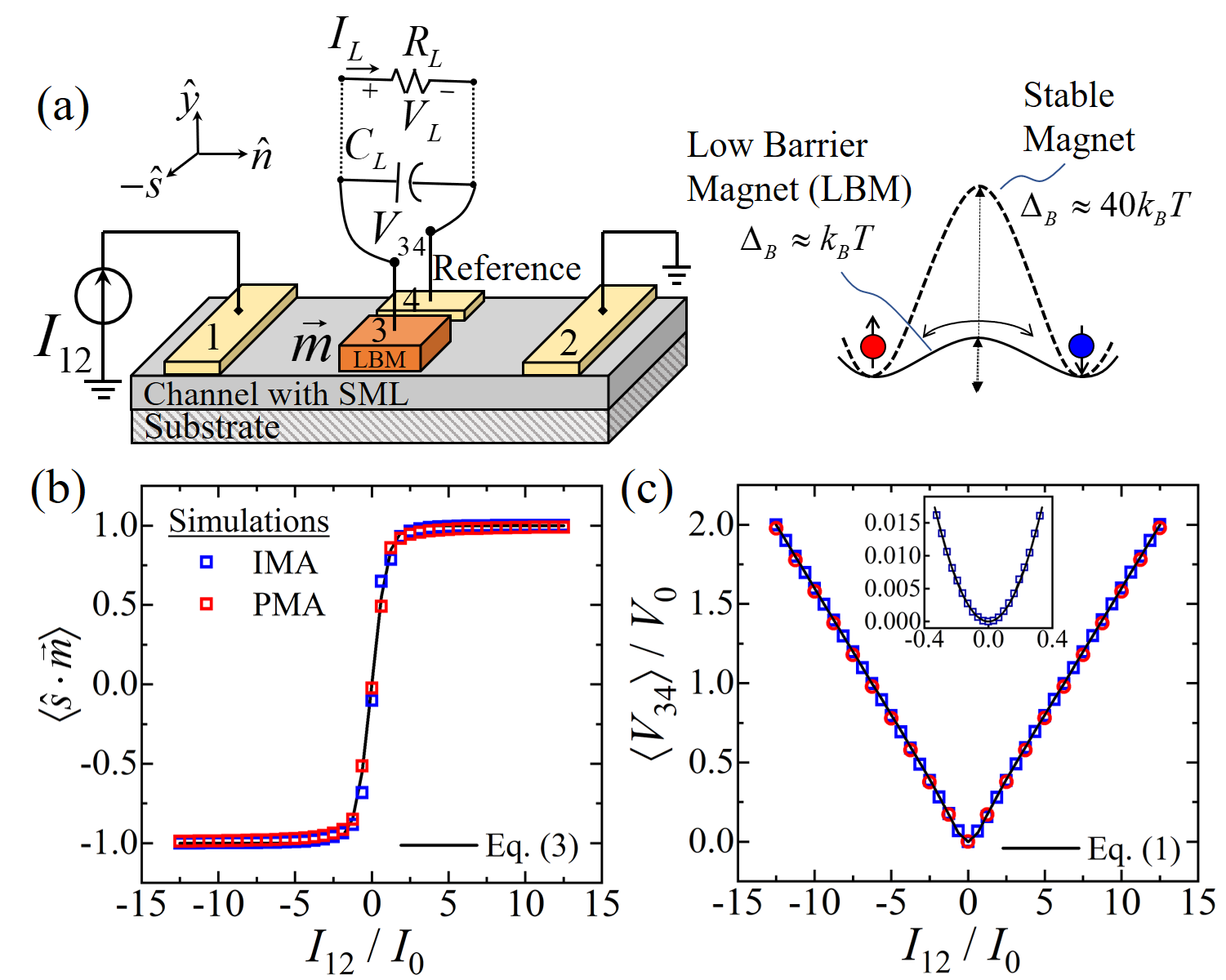
Figure 1: (a) Multi-terminal structure with a low barrier magnet (LBM) on top of a channel with spin-momentum locking (SML). LBM can be of in-plane and perpendicular anisotropies (IMA or PMA). (b) Average magnetization $\langle\hat{s}\cdot\vec{m}\rangle$ of the LBM. (c) Average voltage $\langle V_{34}\rangle$ between the LBM and a reference contact as a function of the input current $I_{12}$. Inset shows zoomed version of $\langle V_{34}\rangle$ for very small input current, which exhibits a parabolic nature. Simulations are compared with Eqs. (1) and (3). $I_{0}$ for IMA and PMA are 80 $\mu$A and 1.6 $\mu$A respectively. Here, $V_{0}=I_{0}R_{B}$.

Note that Eq. (1) is valid all the way from ballistic to diffusive regime of operation Hong et al. (2012); Sayed et al. (2018). We restrict our discussion to linear response where ${V_{34}\left(\vec{m}\right)}$ in Eq. (1) scales linearly with $I_{12}$ and satisfies the Onsager reciprocity relation Jacquod et al. (2012); Sayed et al. (2016)

$$R_{ij,kl}\left(\vec{m}\right)=R_{kl,ij}\left(-\vec{m}\right),$$

with $R_{ij,kl}=V_{kl}/I_{ij}$. The Onsager reciprocity does not require any specific relation between $R_{ij,kl}\left(\vec{m}\right)$ and $R_{ij,kl}\left(-\vec{m}\right)$ in linear response and the phenomenon described by Eq. (1) has been observed on diverse spin-orbit materials e.g. topological insulator (TI) Li et al. (2014); Hus et al. (2017); Liu et al. (2015); Dankert et al. (2015), Kondo insulators Kim et al. (2018), transition metals Pham et al. (2016), semimetals Li et al. (2018), and semiconductors Lee et al. (2018).

To measure Eq. (1) from a highly resistive SML channel (e.g. TI Li et al. (2014); Hus et al. (2017); Liu et al. (2015); Dankert et al. (2015), semiconductor Lee et al. (2018), etc.) using a metallic FM, usually a thin tunnel barrier is inserted at the interface. This tunnel barrier effectively enhances $V_{34}$ by improving $\xi$ Sayed et al. (2016), however, degrades the spin injection into the FM from the SML channel. It has been recently demonstrated Pham et al. (2016) that $V_{34}$ can be measured with metallic FM in direct contact with metallic SML channels (e.g. Pt, Ta, W, etc.), which indicates the possibility of spin-voltage reading (e.g. Pham et al. (2016)) and spin-orbit torque (SOT) writing (e.g. Liu et al. (2012a, b)) of the nano-magnet within same setup with different current magnitudes Sayed et al. (2017).

The energy barrier of a mono-domain magnet is given by $\Delta_{B}=\frac{1}{2}H_{k}M_{s}\Omega$ Sun (2000) where $H_{k}$ is the anisotropy field, $M_{s}$ is the saturation magnetization, and $\Omega$ is the FM volume. For a stable FM, $\Delta_{B}\approx 40\sim 60\;k_{B}T$ and exhibit very long retention time $\tau\propto\exp\left(\Delta_{B}/k_{B}T\right)$ of the magnetization state ($k_{B}:$ Boltzmann constant, $T:$ temperature). LBMs have very small $\tau$ and the $\hat{s}\cdot\vec{m}$ component becomes random within the range $\left\{+1,-1\right\}$ driven by the thermal noise. Experimentally, LBMs have been achieved by lowering the total moment ($M_{s}\Omega$) Vodenicarevic et al. (2017) or by lowering the anisotropy field ($H_{k}$) either by increasing the thickness of a PMA Debashis et al. (2018), or by making a circular IMA with no shape anisotropy Debashis et al. (2016).

At equilibrium ($I_{12}=0$), the time-averaged $\langle\hat{s}\cdot\vec{m}\rangle=0$ for an LBM. For $I_{12}\neq 0$, induced non-equilibrium spins in the channel apply SOT on the LBM and $\langle\hat{s}\cdot\vec{m}\rangle$ follows the accumulated spins, which can be calculated using

$$\langle\hat{s}\cdot\vec{m}\rangle=\dfrac{\displaystyle\int_{\phi=-\pi}^{\phi=\pi}\displaystyle\int_{\theta=0}^{\theta=\pi}\left(\hat{s}\cdot\vec{m}\right)\;\rho\;\sin\theta\;d\theta d\phi}{\displaystyle\int_{\phi=-\pi}^{\phi=\pi}\displaystyle\int_{\theta=0}^{\theta=\pi}\rho\;\sin\theta\;d\theta d\phi}.$$ (2)

where $\rho$ is the probability distribution function of the magnetization of the LBM under a particular $I_{12}$, which can be obtained from the Fokker-Planck equation Brown (1963); Butler et al. (2012). The dependence of $\langle\hat{s}\cdot\vec{m}\rangle$ on $I_{12}$ deduced from Eq. (2) for a particular LBM, can in-principle be any saturating odd-functions e.g. Langevin function for low-barrier PMA (see Appendix A).

We approximate $\langle\hat{s}\cdot\vec{m}\rangle$ in Eq. (2) with a $\tanh$ functional dependence on $I_{12}$, given by

$$\langle\hat{s}\cdot\vec{m}\rangle\approx\tanh\left(\dfrac{I_{12}}{I_{0}}\right),$$ (3)

which is in good agreement with the detailed numerical simulations for both IMA and PMA, as shown in Fig. 1(b). The simulations are carried out within a multi-physics framework Camsari et al. (2015) using our experimentally benchmarked transmission line model for SML Sayed et al. (2018) and stochastic Landau-Lifshitz-Gilbert (s-LLG) model for LBM Camsari et al. (2017) which considers thermal noise. The details of the simulation setup is discussed in Appendix B.

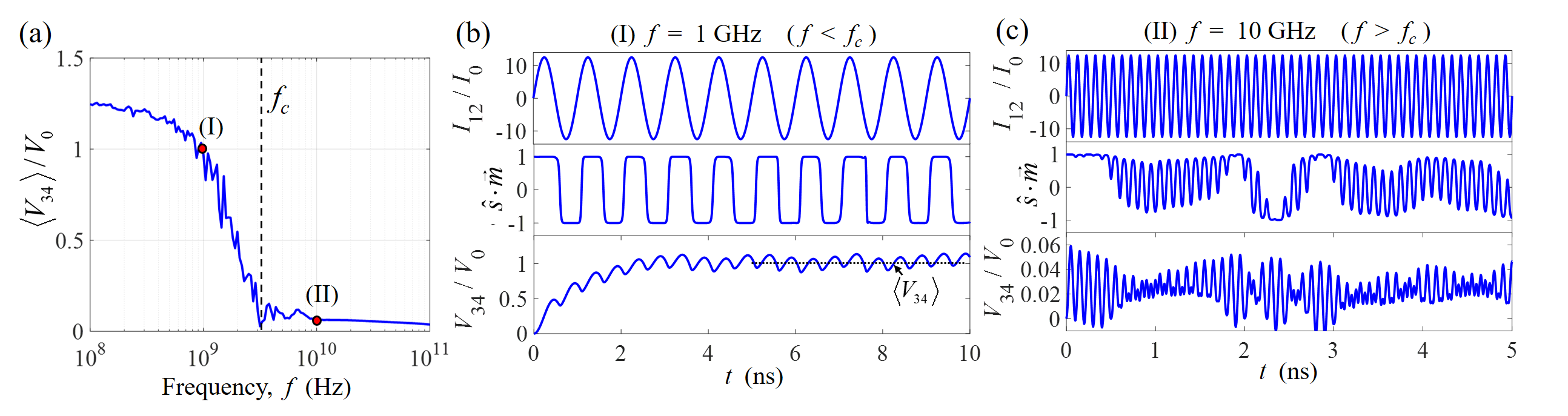
Figure 2: (a) Rectified voltage $\langle V_{34}\rangle$ as a function of the input ac frequency $f$, showing the frequency bandwidth $f_{c}$. We observe the time dynamics of the LBM under input current $I_{12}$ for (b) $f<f_{c}$, where $\hat{s}\cdot\vec{m}$ on average follows $I_{12}$ leading to rectification and (c) $f>f_{c}$, where $\hat{s}\cdot\vec{m}$ struggles to follow $I_{12}$ and yields no net rectification. Results apply to both IMA and PMA. Here, we consider 49 nm $\times$ 61 nm $\times$ 5 nm LBM with $M_{s}=900$ emu/cc. $i_{s0}=\beta i_{c0}=2$ mA.

Here, $I_{0}$ is a parameter that determines the SOT induced magnetization pinning of the LBM. $I_{0}$ depends on the temperature, geometry, and material parameters and much larger for an IMA as compared to a PMA due to the demagnetization field. $I_{12}$ along $\mp\hat{n}$-direction causes the magnetization pinning along $\pm\hat{s}$-direction. In the present discussion, easy axis for PMA is along $\hat{y}$-direction, hence, the pinning occurs along the hard axis. The easy axis of IMA, in principle, can be in any direction on the plane spanned by $\hat{n}$ and $\hat{s}$ and the magnetization pinning along $\hat{s}$-direction should be described by Eq. (3) with a modified $I_{0}$. However, we set the easy axis along $\pm\hat{s}$-direction in our IMA simulations for simplicity.

For a given structure, $I_{0}$ can be determined directly from experiments using a characteristic curve similar to that in Figs. 1(b) or (c). We provide a simple expression using Eq. (2) and considering easy-axis pinning of a PMA magnet (see Appendix A for the derivation), as given by

$${I_{0}}\approx\frac{{6q}}{\hbar}\frac{{{k_{B}}T{\alpha_{g}}}}{\beta},$$ (4)

where $\alpha_{g}$ is the Gilbert damping and $\beta$ is the charge to spin current conversion ratio. Eq. (4) is reasonably valid up to $\Delta_{B}\approx k_{B}T$ and provides the correct order of magnitude up to several $k_{B}T$ (see Appendix A for details). In this discussion, we consider very low energy barrier ($\leq 1k_{B}T$) nano-magnets that do not have bistable states. A higher barrier magnet that exhibits bistable states, in principle could exhibit effects like stochastic resonance Cheng et al. (2010), which is not the subject of the present discussion.

For $|I_{12}|\gg I_{0}$ in Eq. (3), we have $\tanh\left(I_{12}/I_{0}\right)\approx$ $+1$ or $-1$ when $I_{12}>0$ or $I_{12}<0$ respectively. Hence, $I_{12}\times\tanh\left(I_{12}/I_{0}\right)\approx|I_{12}|$. On the other hand, for $|I_{12}|\ll I_{0}$ in Eq. (3), we have $I_{12}\times\tanh\left(I_{12}/I_{0}\right)\approx I_{12}^{2}/I_{0}$. Thus, the time-average of the voltage in Eq. (1) is given by

$$\langle V_{34}\rangle=\begin{cases}\left(\dfrac{{\alpha\xi{p_{0}}{p_{f}}R_{B}}}{{2I_{0}}}\right)\,{I_{12}^{2}},&\text{for $|I_{12}|\ll I_{0}$}\\ \left(\dfrac{{\alpha\xi{p_{0}}{p_{f}}R_{B}}}{{2}}\right)\,{|I_{12}|}.&\text{for $|I_{12}|\gg I_{0}$}\end{cases}$$ (5)

Note that $\langle V_{34}\rangle$ represents the steady-state voltage of the capacitor $C_{L}$ placed between contacts 3 and 4. The relative position between contacts 3 and 4 along $\hat{s}$-direction do not affect Eq. (1), however, a shift in the $\hat{n}$-direction creates an offset due to Ohmic drop Sayed et al. (2017), that should cancel out over averaging in Eq. (5) when an ac $I_{12}$ is applied. For arbitrary $I_{12}$, $\langle V_{34}\rangle$ is always of the same sign leading to a multi-terminal rectification. This observation agrees well with simulation results for IMA and PMA, as shown in Fig. 1(c). For $|I_{12}|\ll I_{0}$, $\langle V_{34}\rangle$ exhibits a parabolic nature (see zoomed inset of Fig. 1(c)), as suggested by Eq. (5). All simulation results presented in this paper are normalized by $I_{0}$, $V_{0}=I_{0}R_{B}$, and $f_{0}=I_{0}/q$ for current, voltage, and frequency, respectively. In all simulations, $M_{t}=100$ which yields $R_{B}=259\Omega$.

III Frequency Bandwidth

The frequency bandwidth of the the multi-terminal rectification is limited by a characteristic frequency $f_{c}$ that is determined by the angular momentum conservation between the spins injected from the SML channel and the spins absorbed by the LBM. We plot the $\langle V_{34}\rangle$ as a function of the frequency $f$ of the ac $I_{12}=i_{c0}\,\sin\left(2\pi ft\right)$ (see Fig. 2(a)) while other parameters are kept constant in our simulations. Note that $\langle V_{34}\rangle$ is relatively constant in the low frequency region and degrades significantly for $f>f_{c}$. We have defined $f_{c}$ as the frequency where $\langle V_{34}\rangle$ degrades by an order of magnitude compared to the region where $\langle V_{34}\rangle$ vs. $f$ is relatively flat.

We observe the time-dynamics of $\hat{s}\cdot\vec{m}$ and $V_{34}$ for the two cases indicated with red-dots in Fig. 2(a): (I) $f<f_{c}$ and (II) $f>f_{c}$. For the first case, $I_{12}$ is slow enough that the injected spins from SML channel into the LBM satisfies the angular momentum conservation and $\hat{s}\cdot\vec{m}$ follows the $I_{12}$ at the same frequency, as shown in Fig. 2(b). This leads to a rectified voltage $V_{34}$ that charges up the capacitor $C_{L}$ to the steady-state value $\langle V_{34}\rangle$. The ripples observed in $V_{34}$ is similar to those in conventional rectifiers and gets attenuated for increased $C_{L}$. For the latter case, $\hat{s}\cdot\vec{m}$ struggles to follow $I_{12}$ (see Fig. 2(c)) since the spins injected from the SML channel to the LBM is fast enough that they do not satisfy the angular momentum conservation. $\hat{s}\cdot\vec{m}$ has no correlation with $I_{12}$, as a result, there is no rectification that charges up $C_{L}$ to a steady dc voltage.

We obtain an empirical expression for $f_{c}$ from the detailed s-LLG simulations using a broad range of parameter values, given by

$$2\pi{f_{c}}=\dfrac{i_{s0}}{{2q{N_{s}}}},$$ (6)

where the injected spin current amplitude $i_{s0}=\beta i_{c0}$, $N_{s}=M_{s}\Omega/\mu_{B}$ is the total number of spins in LBM and $\mu_{B}$ is the Bohr magneton. The functional dependence of $f_{c}$ on $i_{s0}$ and $N_{s}$ is very similar to the switching delay for stable magnets Behin-Aein et al. (2011) that also arises from the principles of angular momentum conservation. Note that Eq. (6) is valid for both IMA and PMA.

We show comparison between Eq. (6) and simulation results in Fig. 3. The simulation data points shown on Fig. 3 are extracted from a plot similar to Fig. 2(a). Eq. (6) shows good agreement with the simulation for LBMs having IMA with easy-axis pinning and PMA with hard-axis pinning (see Figs. 3(a)-(b)). Fig. 3(a) shows that $f_{c}$ scales linearly with $i_{s0}$. A similar scenario has been reported Locatelli et al. (2014) for a stochastic MTJ oscillator made with relatively lower-barrier free magnetic layer. According to Eq. (6) and detailed simulations, the conclusion that $f_{c}\propto i_{s0}$ seems valid even if $i_{s0}$ changes by orders of magnitude. Moreover, Fig. 3(b) shows that $f_{c}$ scales inversely proportional to the $N_{s}$ which depends only on $M_{s}\Omega$ of the magnet and independent of the magnetic anisotropy. Eq. (6) could be useful for recent interest on LBM based applications e.g. stochastic oscillators Locatelli et al. (2014), random number generators Parks et al. (2018); Vodenicarevic et al. (2017), probabilistic spin logic Camsari et al. (2017); Mizrahi et al. (2018), etc.

IV Applications: RF Detection and Energy Harvesting

The proposed all-metallic structure can find useful applications like rf detection and energy harvesting. In this section, we show that the low-barrier nature of the magnet can lead to very high rf detection sensitivity without any external bias, comparable to those observed in state-of-the-art technologies under an external bias. We provide a simple model for no-bias sensitivity which provides insight into the design of a high-sensitivity device. This could be of interest for rf detection from weak sources typically proposed to sense with quantum sensors (see, e.g., House et al. (2015); Gely et al. (2019)).We further argue that the proposed structure can extract useful energy from the ambient rf energy, especially from the weak sources where standard technologies may not operate.

It can be seen from Eq. (5) that $\langle V_{34}\rangle$ scales $\propto\sqrt{P_{in}}$ when $\max\left(I_{12}\right)\gg I_{0}$, where $P_{in}=\frac{1}{T}\int_{0}^{T}I_{12}^{2}\left(t\right)R_{12}\,dt$, $T=1/f$, and $R_{12}$ is the channel resistance. However, for $\max\left(I_{12}\right)\ll I_{0}$, $\langle V_{34}\rangle$ scales $\propto P_{in}$ with a constant slope given by

$$\dfrac{d\langle V_{34}\rangle}{dP_{in}}=\dfrac{{\alpha\xi{p_{0}}{p_{f}}}}{{2}}\dfrac{{R_{B}}}{{{I_{0}}{R_{12}}}}.$$ (7)

The derivation is given in Appendix C. The quantity in Eq. (7) is often considered as the sensitivity of rf detectors Miwa et al. (2013); Fang et al. (2016); Zhang et al. (2018). Recently, Magnetic Tunnel Junction (MTJ) diodes with stable magnet as free layer and under an external dc current bias have demonstrated orders of magnitude higher sensitivity compared to the state-of-the-art Schottky diodes Miwa et al. (2013); Fang et al. (2016); Zhang et al. (2018). However, the reported no-bias sensitivity is lower or comparable to that of semiconductor diodes. Eq. (7) indicates that the no-external-bias sensitivity can be very high within the all-metallic structure in Fig. 1(a) when designed to have very low $I_{0}$, enabling highly sensitive ‘passive’ rf detection. With $\alpha_{g}=0.01$ and $T=300$ K we have $I_{0}\approx 0.37\mu$A$/\beta$ from Eq. (4). For a Py LBM of dimension of 49 nm $\times$ 61 nm $\times$ 5 nm (see Ref. Debashis et al. (2018)) and 2 nm thick Pt channel, $\beta$ can be $\sim 2$ as estimated from the charge to spin conversion ratio reported in Ref. Liu et al. (2012b), yielding $I_{0}\approx 0.18$ $\mu$A. Note that $\beta$ can be much higher based on the geometry and the choice of the SML material.

For Bi₂Se₃ and Pt, we roughly estimate the sensitivity as 21,000 and 860 mV/mW respectively, assuming 2D SML channel of width $w=$ 210 nm and length $L=$ 500 nm. These estimations were done based on Eq. (7) using: (i) $R_{B}=$ 259 $\Omega$ (Bi₂Se₃) and 58 $\Omega$ (Pt), (ii) $R_{ch}\approx$ $6.5$ k$\Omega$ (Bi₂Se₃) and $\sim 3$ k$\Omega$ (Pt), (iii) $p_{0}\approx$ 0.6 (Bi₂Se₃) and 0.05 (Pt) (see Ref. Sayed et al. (2017)), and (iv) $p_{f}\approx 0.5$ Lee et al. (2018). We have assumed $\xi\approx 1$ and the quoted estimations will be lower for higher shunting. $R_{B}$ has been estimated using $M_{t}=k_{F}w/\pi$, where $k_{F}=1.5$ nm^-1 (Bi₂Se₃) and $6.7$ nm^-1 (Pt) Sayed et al. (2017). The channel resistance has been estimated using $R_{ch}=R_{B}(L+\lambda)/\lambda$ with mean free path $\lambda$ of 20 nm (Bi₂Se₃ Wang et al. (2016)) and 10 nm (Pt Fischer et al. (1980)), respectively. More detailed analysis and performance evaluation considering signal-to-noise ratio we leave for future work.

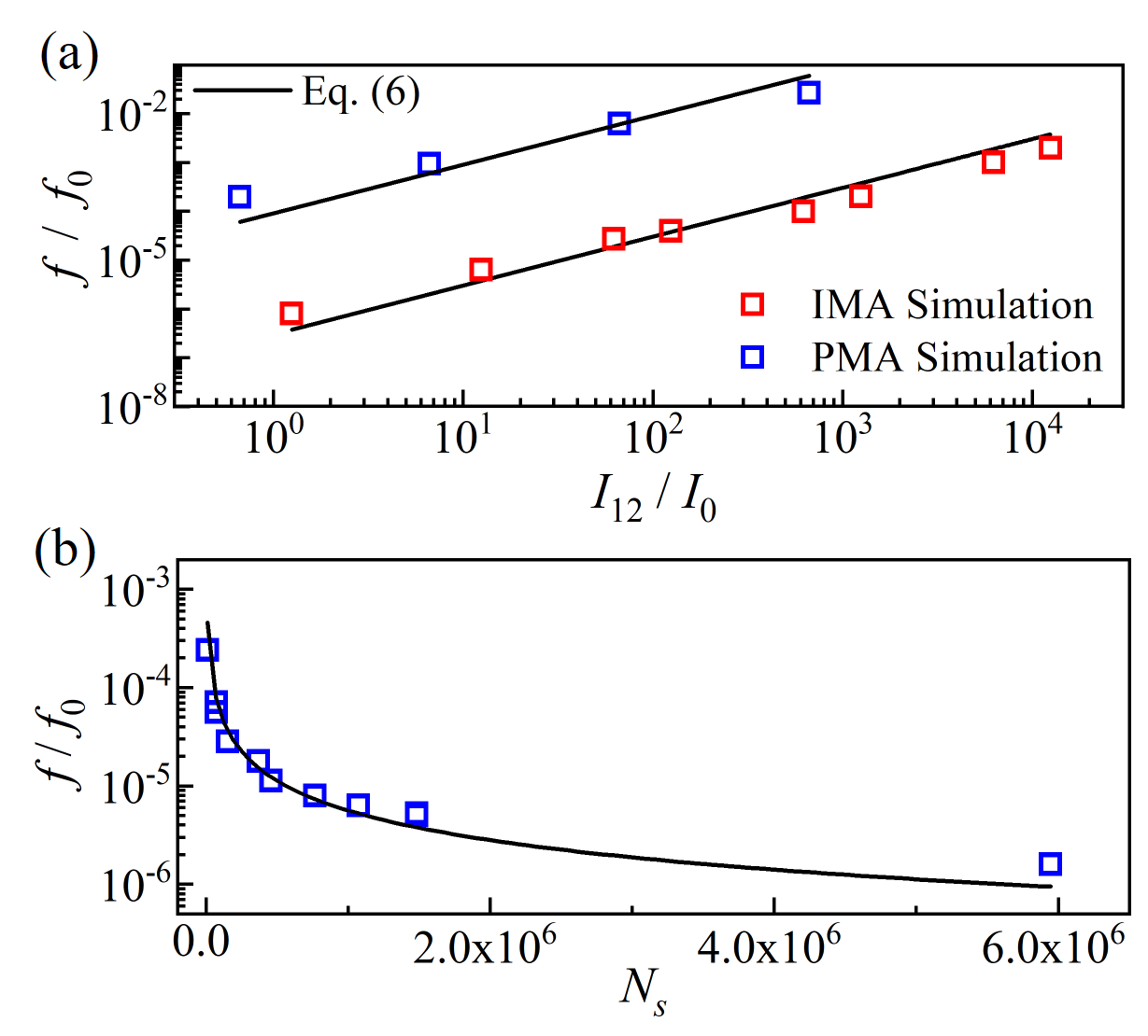
Figure 3: Characteristic frequency $f_{c}$ is (a) proportional to $i_{c0}$ ($N_{s}=$ $10^{4}$ and $10^{6}$ for PMA and IMA respectively) and (b) inversely proportional to $N_{s}$. Here, $f_{0}=I_{0}/q$.

With proper materials and geometry, it may be possible to extract usable energy from such rectification of rf signals, especially from weak ambient sources. The dc power $P_{L}=V_{L}I_{L}$ extracted by an arbitrary load $R_{L}$ is limited by the equivalent resistance $R_{34}$ between contacts 3 and 4. The maximum efficiency of such rf to dc power conversion occurs for $\max\left(I_{12}\right)\gg I_{0}$, given by

$$\eta_{\max}=\dfrac{P_{L,\max}}{P_{in}}=\left(\dfrac{{\alpha\xi{p_{0}}{p_{f}}}}{\sqrt{2}{\pi}}\right)^{2}\dfrac{R_{B}}{{R_{12}}}\dfrac{R_{B}}{{R_{34}}}.$$ (8)

The derivation is given in Appendix D. Note that the maximum efficiency is independent of $I_{0}$. Assuming $R_{eq}=10R_{B}$ for enhanced $\xi$, we estimate the maximum efficiency to be 0.001% for Bi₂Se₃ and 3$\times$10^-6% for Pt even with $P_{in}$ in the $\sim$pW range given $I_{0}\leq 0.18\mu$A. MTJ diodes recently demonstrated rf energy harvesting with similar efficiency Fang et al. (2019), however, the input power was in the $\mu$W range. Such MTJs should achieve reasonable efficiency at lower input power if the stable free layer is replaced with an LBM.

V Conclusion

In conclusion, we predict multi-terminal rectification in an all-metallic structure that comprises a spin-orbit material exhibiting spin-momentum locking (SML) and a low-energy barrier magnet (LBM) having either in-plane or perpendicular anisotropy (IMA or PMA). The discussion of such multi-terminal rectification was limited in the linear response regime of transport and the non-linearity occurs due to the spin-orbit torque driven magnetization dynamics of the LBM. We draw attention to a frequency band of the rectification which can be understood in terms of angular momentum conservation within the LBM. For a fixed spin-current from the SML channel, the frequency band is same for LBMs with IMA and PMA, as long as they have the same total magnetic moment for a given volume. We further discuss possible applications of the wideband rectification as highly sensitive passive rf detectors and as energy harvesters from ambient sources.

Appendix A Average Magnetization of Low-Barrier Magnets and Magnetization Pinning Current

This section discusses the pinning current of a LBM and derives Eqs. (3)-(4), starting from the steady-state solution of the Fokker-Planck Equation.

We start from the steady-state solution of probability distribution from Fokker-Planck Equation assuming a magnet with perpendicular magnetic anisotropy (PMA) (see Eq. (4.3) in Ref. Butler et al. (2012)), given by

$$\rho\left(m_{z}\right)=\dfrac{1}{{\rm Z}}\exp\left[-\dfrac{\Delta_{B}}{k_{B}T}\left(1-m_{z}^{2}+2\left(\dfrac{H_{ext}}{H_{k}}+\dfrac{i_{s}}{I_{s0}}\right)m_{z}\right)\right],$$ (9)

where $\rm Z$ is a normalizing factor, $m_{z}$ is the magnetization along easy-axis ($\hat{s}\cdot\vec{m}$ in the present discussion), $\Delta_{B}=H_{k}M_{s}\Omega/2$ is the energy barrier of a magnet with anisotropy field $H_{k}$, saturation magnetization $M_{s}$, and volume $\Omega$, $k_{B}$ is the Boltzmann constant, $T$ is the temperature, $H_{ext}$ is the external magnetic field along the easy-axis, $i_{s}$ is the $z$-polarized spin current injected into the magnet, and $I_{s0}$ is the critical spin current for magnetization switching Sun (2000); Sayed et al. (2017) for a magnet with PMA, given by

$$I_{s0}=\dfrac{4q}{\hbar}\Delta_{B}\alpha_{g},$$ (10)

where $\hbar=h/(2\pi)$ and $\alpha_{g}$ is the Gilbert damping constant.

We consider the case with no external field i.e. $H_{ext}=0$ which from Eqs. (9) and (10) gives

$$\rho\left(m_{z}\right)=\dfrac{1}{{\rm Z}}\exp\left(-\dfrac{\Delta_{B}}{k_{B}T}\left(1-m_{z}^{2}\right)-\left(\dfrac{i_{s}}{\dfrac{2q}{\hbar}k_{B}T\alpha_{g}}\right)m_{z}\right).$$ (11)

We consider very low energy barrier magnet i.e. $\frac{\Delta_{B}}{k_{B}T}\rightarrow 0$, which in Eq. (11) yields

$$\rho\left(m_{z}\right)=\dfrac{1}{{\rm Z}}\exp\left(-\dfrac{i_{s}}{\dfrac{2q}{\hbar}k_{B}T\alpha_{g}}m_{z}\right).$$ (12)

The steady-state average $\langle m_{z}\rangle$ is defined as (see Eq. (2))

$$\langle m_{z}\rangle=\dfrac{\int_{\phi=-\pi}^{\phi=\pi}\int_{\theta=0}^{\theta=\pi}m_{z}\;\rho(m_{z})\;\sin\theta\;d\theta d\phi}{\int_{\phi=-\pi}^{\phi=\pi}\int_{\theta=0}^{\theta=\pi}\rho(m_{z})\;\sin\theta\;d\theta d\phi},$$ (13)

with $\left(m_{z},m_{x},m_{y}\right)\equiv\left(\cos\theta,\sin\theta\cos\phi,\sin\theta\sin\phi\right)$. Combining Eq. (13) with Eq. (12) we get the long time averaged magnetization $\langle m_{z}\rangle$ for a very low barrier PMA without external magnetic field as

$$\langle m_{z}\rangle=\coth\left(\dfrac{i_{s}}{\dfrac{2q}{\hbar}k_{B}T\alpha_{g}}\right)-\dfrac{\dfrac{2q}{\hbar}k_{B}T\alpha_{g}}{i_{s}},$$ (14)

which is a Langevin function $L(x)$ of $x\equiv{i_{s}}/\left({\frac{2q}{\hbar}k_{B}T\alpha_{g}}\right)$.

Note that Eq. (14) was derived assuming $\frac{\Delta_{B}}{k_{B}T}\rightarrow 0$, however, the expression remains reasonably valid up to ${\Delta_{B}}\approx{k_{B}T}$. We have compared Eq. (14) with numerical calculations directly from Eqs. (11) and (13) for $\Delta_{B}=0.1k_{B}T$ (see Fig. 4(a)) and $k_{B}T$ (see Fig. 4(b)) respectively, which shows reasonably good agreement. For $\Delta_{B}>{k_{B}T}$, the simple expression in Eq. (14) deviates from Eqs. (11) and (13).

For an estimation of the pinning spin current we can approximate the Langevin function $L(x)\approx\tanh\dfrac{x}{3}$, hence

$$\langle m_{z}\rangle\approx\tanh\left(\dfrac{i_{s}}{\dfrac{6q}{\hbar}k_{B}T\alpha_{g}}\right).$$ (15)

Note that $i_{s}$ from SML materials are related to input charge current $i_{c}$ with a conversion factor $\beta$ given by

$$i_{s}=\beta i_{c}.$$ (16)

Combining Eq. (16) with Eq. (15) yields

$$\langle m_{z}\rangle\approx\tanh\left(\dfrac{i_{c}}{\dfrac{6qk_{B}T\alpha_{g}}{\hbar\beta}}\right).$$ (17)

Comparing Eq. (17) with Eq. (3) yields

$$I_{0}\approx\dfrac{6qk_{B}T\alpha_{g}}{\hbar\beta},$$

which gives the expression in Eq. (4).

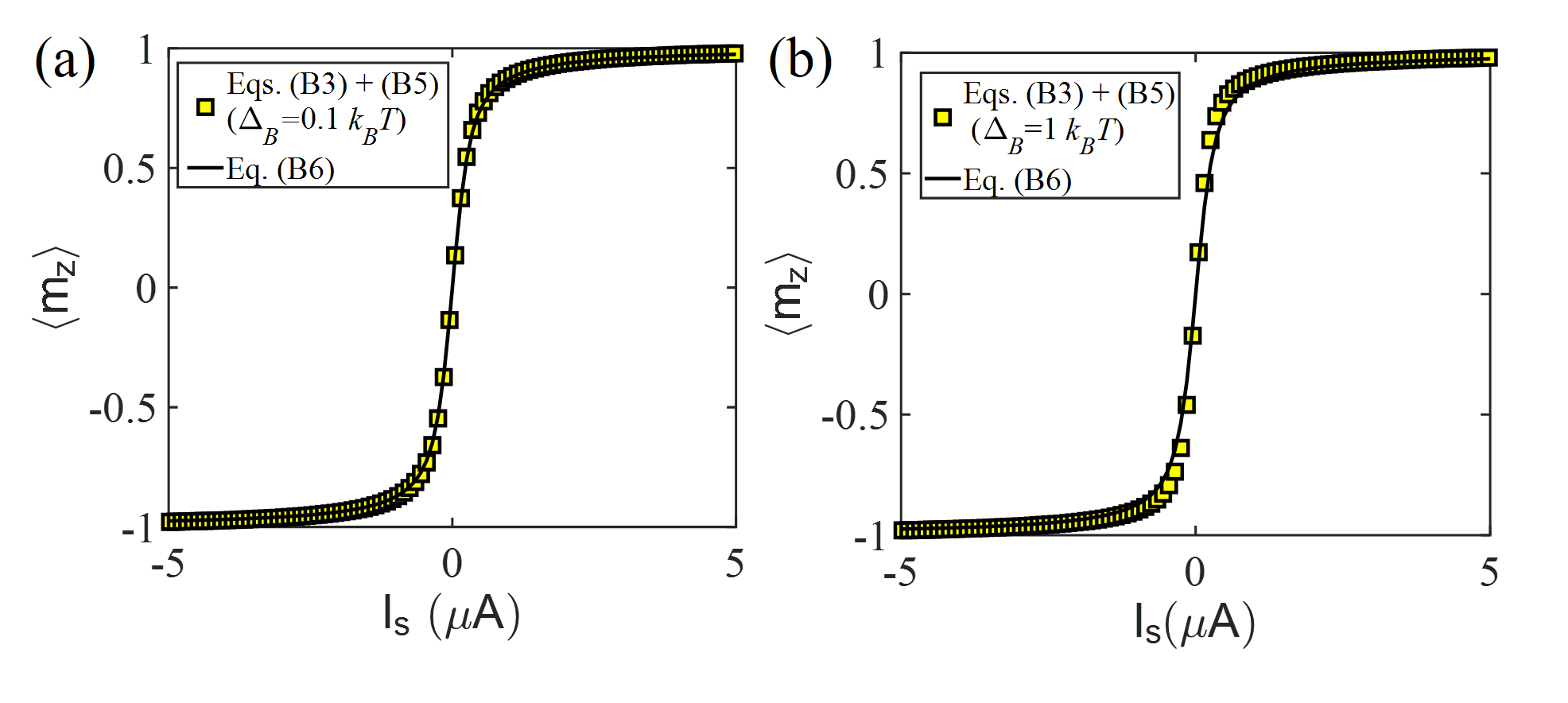
Figure 4: Comparison of simple expression in Eq. (14) which assumes $\Delta_{B}\rightarrow 0$ with the numerical calculation from Eqs. (11) and (13) for (a) $\Delta_{B}=0.1k_{B}T$ and (b) $\Delta_{B}=1k_{B}T$. This comparison indicates that Eq. (14) is reasonably valid for $0\leq\Delta_{B}\leq 1k_{B}T$.

Appendix B Simulation Setup

This section provides the details of the simulation setup in SPICE that was used to analyze the proposed rectifier.

We have discretized the structure in Fig. 1(a) into 100 small sections and represented each of the small sections with the corresponding circuit model. Note that each of the nodes in Fig. 5 are two component: charge ($c$) and $z$-component of spin ($s$). We have connected the charge and spin terminals of the models for all the small sections in a modular fashion using standard circuit rules as shown in Fig. 5. The models are connected in a series to reconstruct the structure along length direction. We have two of such parallel chains to take into account the structure along width direction and the two chains represent the area under the LBM and the reference NM respectively. The SML block with LBM is connected to a s-LLG block which takes the spin current from the SML block as input and self-consistently solves for $m_{z}$ and feeds back to the SML block.

The contacts (1, 2, 3, and 4) in this discussion are point contacts. The polarization of contacts 1, 2, and 4 are $p_{f}=0$ since they represent normal metals. Polarization of contact 3 is 0.8 which represents an LBM. We set the total number of modes $M+N$ in the channel to be 100. We have assumed that the reflection with spin-flip scattering mechanism is dominant in the channel i.e. $r_{s1,2}\gg r,t_{s}$. The scattering rate per unit mode was set to 0.04 per lattice point.

We apply the charge open and spin ground boundary condition at the two boundaries given by

$${\left\{{\begin{array}[]{*{20}{c}}{{i_{c}}}\\ {{v_{s}}}\end{array}}\right\}_{L}}=\left\{{\begin{array}[]{*{20}{c}}0\\ 0\end{array}}\right\},\,\,\,\,\text{and}\,\,{\left\{{\begin{array}[]{*{20}{c}}{{i_{c}}}\\ {{v_{s}}}\end{array}}\right\}_{R}}=\left\{{\begin{array}[]{*{20}{c}}0\\ 0\end{array}}\right\}.$$ (18)

Here, $i_{c}$ and $v_{s}$ indicates boundary charge current and boundary spin voltage. Indices $L$ and $R$ indicate left and right boundaries respectively.

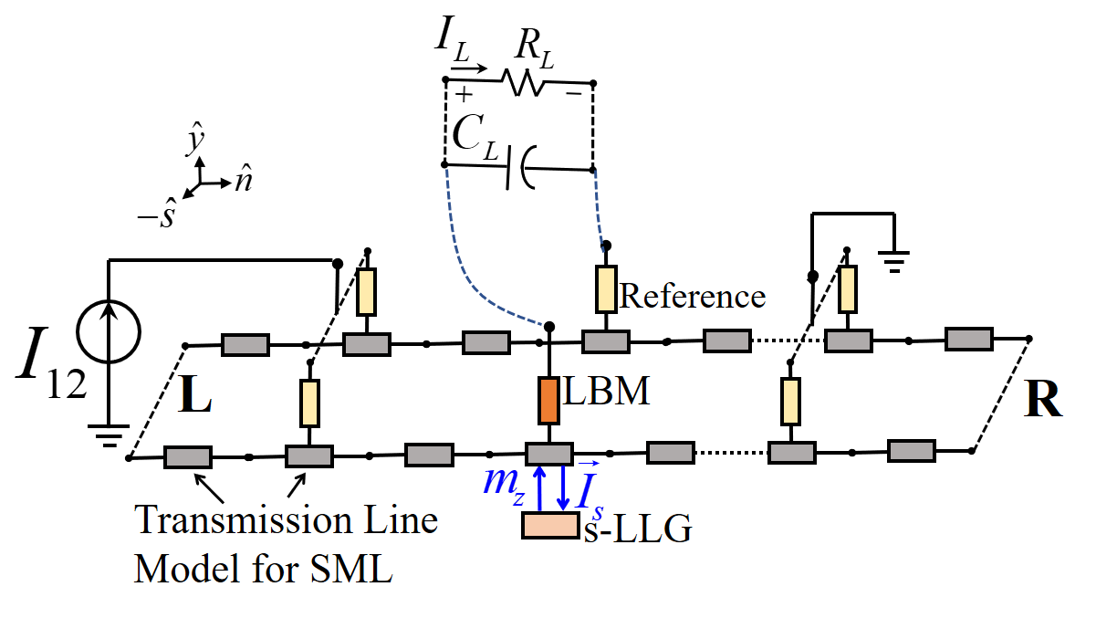
Figure 5: SPICE simulation setup for the structure shown in Fig. 1(a). SML channel is modeled by connecting SPICE compatible transmission line model Sayed et al. (2018) in a distributed manner. The LBM is modeled with stochastic Landau-Lifshitz-Gilbert (s-LLG) SPICE model Camsari et al. (2017).

Both charge and spin terminals of contact 1 and 2 and the two boundaries of the two parallel model chains are connected together. We apply a current $i_{c}$ at the charge terminal of contact 1 and make the spin terminal grounded to take into account the spin relaxation process in the contact. We ground both charge and spin terminals of contact 2. The boundary conditions of contacts 1 and 2 are given by

$${\left\{{\begin{array}[]{*{20}{c}}{{i_{c}}}\\ {{v_{s}}}\end{array}}\right\}_{1}}=\left\{{\begin{array}[]{*{20}{c}}i_{c}\\ 0\end{array}}\right\},\,\,\,\,\text{and}\,\,{\left\{{\begin{array}[]{*{20}{c}}{{v_{c}}}\\ {{v_{s}}}\end{array}}\right\}_{2}}=\left\{{\begin{array}[]{*{20}{c}}0\\ 0\end{array}}\right\}.$$ (19)

We place a capacitor $C_{L}$ and load $R_{L}$ across the charge terminals of contacts 3 and 4. The spin terminals of contacts 3 and 4 are grounded. The boundary conditions of the contacts 3 and 4 are given by

$${\left\{{\begin{array}[]{*{20}{c}}{{i_{c}}}\\ {{v_{s}}}\end{array}}\right\}_{3}}=\left\{{\begin{array}[]{*{20}{c}}0\\ 0\end{array}}\right\},\,\,\,\,\text{and}\,\,{\left\{{\begin{array}[]{*{20}{c}}{{i_{c}}}\\ {{v_{s}}}\end{array}}\right\}_{4}}=\left\{{\begin{array}[]{*{20}{c}}0\\ 0\end{array}}\right\}.$$ (20)

Appendix C Sensitivity

This section discusses the detailed derivation of the sensitivity model in Eq. (7).

We start from Eq. (1) with $\vec{m}(t)$ being the instantaneous magnetization of the LBM. and calculate the average as

$$\langle V_{34}\rangle =\dfrac{1}{T}\int_{0}^{T}V_{34}\,dt$$ (21)

$$=\dfrac{1}{T}\dfrac{{\alpha\xi{p_{0}}{p_{f}}}}{{2{G_{B}}}}\int_{0}^{T}\tanh\left(\dfrac{I_{12}(t)}{I_{0}}\right)I_{12}(t)\,dt.$$

Note that the timed average of the random fluctuation in LBM is zero. Here, $G_{B}=1/R_{B}$.

We apply an alternating current as input, given by

$$I_{12}(t)=i_{c0}\sin\left(\dfrac{2\pi t}{T}\right),$$ (22)

The average ac input power applied to the channel with resistance $R_{12}$ is given by

$$P_{in} =\frac{1}{T}\int_{0}^{T}I_{12}^{2}(t)R_{12}\,dt$$ (23)

$$=\frac{i_{c0}^{2}R_{12}}{T}\int_{0}^{T}\sin^{2}\left(\dfrac{2\pi t}{T}\right)\,dt$$

$$=\left(\frac{i_{c0}}{\sqrt{2}}\right)^{2}R_{12}.$$

C.1 Case I: $i_{c0}\gg I_{0}$

For $i_{c0}\gg I_{0}$, we get $\tanh\left(I_{12}(t)/I_{0}\right)\approx+1$ when $I_{12}(t)>0$ and $\tanh\left(I_{12}(t)/I_{0}\right)\approx-1$ when $I_{12}(t)<0$. Thus we have

$$\tanh\left(\dfrac{I_{12}(t)}{I_{0}}\right)\times I_{12}(t)\approx|I_{12}(t)|,$$

and from Eq. (21), we get

$$\langle V_{34}\rangle =\dfrac{1}{T}\dfrac{{\alpha\xi{p_{0}}{p_{f}}}}{{2{G_{B}}}}\int_{0}^{T}|I_{12}(t)|\,dt$$ (24)

$$=\dfrac{1}{T}\dfrac{{\alpha\xi{p_{0}}{p_{f}}}}{{2{G_{B}}}}{i}_{c0}\int_{0}^{T}\left|\sin\left(\dfrac{2\pi t}{T}\right)\right|\,dt$$

$$=\dfrac{1}{T}\dfrac{{\alpha\xi{p_{0}}{p_{f}}}}{{2{G_{B}}}}{i}_{c0}\int_{0}^{\frac{T}{2}}\sin\left(\dfrac{2\pi t}{T}\right)\,dt$$

$$+\dfrac{1}{T}\dfrac{{\alpha\xi{p_{0}}{p_{f}}}}{{2{G_{B}}}}{i}_{c0}\int_{\frac{T}{2}}^{T}-\sin\left(\dfrac{2\pi t}{T}\right)\,dt$$

$$=\dfrac{{\alpha\xi{p_{0}}{p_{f}}}}{{2{G_{B}}}}\times\dfrac{2}{\pi}{i}_{c0}.$$

We write Eq. (24) as

$$\langle V_{34}\rangle=\dfrac{{\alpha\xi{p_{0}}{p_{f}}}}{{\pi{G_{B}}}}\times\dfrac{\sqrt{2}}{\sqrt{R_{12}}}\times\sqrt{P_{in}},$$ (25)

and the sensitivity is given by

$$\dfrac{d\langle V_{34}\rangle}{dP_{in}}=\dfrac{{\alpha\xi{p_{0}}{p_{f}}}}{{\pi{G_{B}}}}\times\dfrac{1}{\sqrt{2R_{12}}}\times\dfrac{1}{\sqrt{P_{in}}}.$$ (26)

The sensitivity for $i_{c0}\gg I_{0}$ decreases inversely proportional to $\sqrt{P_{in}}$. Sensitivity increases for decreasing $P_{in}$ and eventually saturates to a maximum value for $i_{c0}\ll I_{0}$.

C.2 Case II: $i_{c0}\ll I_{0}$

For $i_{c0}\ll I_{0}$, we get $\tanh\left(I_{12}(t)/I_{0}\right)\approx I_{12}(t)/I_{0}$. Thus from Eq. (21), we get

$$\langle V_{34}\rangle =\dfrac{1}{T}\dfrac{{\alpha\xi{p_{0}}{p_{f}}}}{{2{G_{B}}I_{0}}}\int_{0}^{T}I_{12}^{2}(t)\,dt$$ (27)

$$=\dfrac{1}{T}\dfrac{{\alpha\xi{p_{0}}{p_{f}}}}{{2{G_{B}}}}\dfrac{{i}_{c0}^{2}}{I_{0}}\int_{0}^{T}\sin^{2}\left(\dfrac{2\pi t}{T}\right)\,dt$$

$$=\dfrac{{\alpha\xi{p_{0}}{p_{f}}}}{{2{G_{B}}}}\times\dfrac{\left(i_{c0}/\sqrt{2}\right)^{2}}{I_{0}}.$$

We write Eq. (27) as

$$\langle V_{34}\rangle=\dfrac{{\alpha\xi{p_{0}}{p_{f}}}}{{2{G_{B}}R_{12}I_{0}}}P_{in},$$ (28)

and the sensitivity is given as

$$\dfrac{d\langle V_{34}\rangle}{dP_{in}}=\dfrac{{\alpha\xi{p_{0}}{p_{f}}}}{{2{G_{B}}R_{12}I_{0}}},$$ (29)

which gives the maximum sensitivity in Eq. (7).

Appendix D Power Conversion Efficiency

This section discusses the ac to dc power conversion efficiency and provides the details of derivation of Eq. (8).

Under the no load condition ($R_{L}\rightarrow\infty$), we have the open circuit dc voltage from Eq. (28) for $i_{c0}\ll I_{0}$

$$\langle V_{34}\rangle=\dfrac{{\alpha\xi{p_{0}}{p_{f}}}}{{2{G_{B}}R_{12}I_{0}}}P_{in},$$

and from Eq. (25) we know that for $i_{c0}\gg I_{0}$

$$\langle V_{34}\rangle=\dfrac{{\alpha\xi{p_{0}}{p_{f}}}}{{\pi{G_{B}}}}\times\dfrac{\sqrt{2}}{\sqrt{R_{12}}}\times\sqrt{P_{in}}.$$

Under the short circuit condition ($R_{L}\rightarrow 0$), we have the short circuit dc current $I_{L}|_{R_{L}\rightarrow 0}=\langle V_{34}\rangle/R_{34}$, where $R_{34}$ is the equivalent resistance between the LBM and the reference NM.

The maximum power transferred to the load is given by

$$P_{L,\max}=\dfrac{1}{4}\times V_{L}|_{R_{L}\rightarrow\infty}\times I_{L}|_{R_{L}\rightarrow 0}=\dfrac{\langle V_{34}\rangle^{2}}{4R_{34}}.$$ (30)

which yields

$$P_{L,\max} =\left(\dfrac{{\alpha\xi{p_{0}}{p_{f}}}}{{2{G_{B}}R_{12}I_{0}}}\right)^{2}\dfrac{P_{in}^{2}}{4R_{34}}\;\;\;\text{for}\;\;i_{c0}\ll I_{0}$$ (31)

$$=\left(\dfrac{{\alpha\xi{p_{0}}{p_{f}}}}{{\pi{G_{B}}}}\right)^{2}\dfrac{P_{in}}{{2R_{12}R_{34}}}\;\;\;\text{for}\;\;i_{c0}\gg I_{0}.$$

The ac to dc power conversion efficiency is given by

$$\eta=\dfrac{dP_{L,\max}}{dP_{in}} =\left(\dfrac{{\alpha\xi{p_{0}}{p_{f}}}}{{2{G_{B}}R_{12}I_{0}}}\right)^{2}\dfrac{P_{in}}{2R_{34}}\;\;\;\text{for}\;\;i_{c0}\ll I_{0}$$ (32)

$$=\left(\dfrac{{\alpha\xi{p_{0}}{p_{f}}}}{{\pi{G_{B}}}}\right)^{2}\dfrac{1}{{2R_{12}R_{34}}}\;\;\;\text{for}\;\;i_{c0}\gg I_{0}.$$

Note that $\eta$ increases with input ac power $P_{in}$ and reaches a maximum when $i_{c0}\gg I_{0}$ given by

$$\eta_{\max}=\left(\dfrac{{\alpha\xi{p_{0}}{p_{f}}}}{{\pi{G_{B}}}}\right)^{2}\dfrac{1}{{2R_{12}R_{34}}}.$$

References

- Liu et al. (2012a) L. Liu, C.-F. Pai, Y. Li, H. W. Tseng, D. C. Ralph, and R. A. Buhrman, “Spin-torque switching with the giant spin hall effect of tantalum,” Science 336, 555–558 (2012a).
- Liu et al. (2012b) L. Liu, O. J. Lee, T. J. Gudmundsen, D. C. Ralph, and R. A. Buhrman, “Current-induced switching of perpendicularly magnetized magnetic layers using spin torque from the spin hall effect,” Phys. Rev. Lett. 109, 096602 (2012b).
- Li et al. (2014) C. H. Li, O. M. van ’t Erve, J. T. Robinson, Y. Liu, L. Li, and J. B. T., “Electrical detection of charge-current-induced spin polarization due to spin-momentum locking in bi2se3,” Nature Nanotechnol. 9, 20325 (2014).
- Hus et al. (2017) S. M. Hus, X.-G. Zhang, G. D. Nguyen, W. Ko, A. P. Baddorf, Y. P. Chen, and A.-P. Li, “Detection of the spin-chemical potential in topological insulators using spin-polarized four-probe stm,” Phys. Rev. Lett. 119, 137202 (2017).
- Liu et al. (2015) L. Liu, A. Richardella, I. Garate, Y. Zhu, N. Samarth, and C.-T. Chen, “Spin-polarized tunneling study of spin-momentum locking in topological insulators,” Phys. Rev. B 91, 235437 (2015).
- Dankert et al. (2015) A. Dankert, J. Geurs, M. V. Kamalakar, S. Charpentier, and S. P. Dash, “Room temperature electrical detection of spin polarized currents in topological insulators,” Nano Lett. 15, 7976–7981 (2015).
- Pham et al. (2016) V. T. Pham, L. Vila, G. Zahnd, A. Marty, W. Savero-Torres, M. Jamet, and J.-P. Attané, “Ferromagnetic/nonmagnetic nanostructures for the electrical measurement of the spin hall effect,” Nano Lett. 16, 6755–6760 (2016).
- Lee et al. (2018) J.-H. Lee, H.-J. Kim, J. Chang, S. H. Han, H.-C. Koo, S. Sayed, S. Hong, and S. Datta, “Multi-terminal spin valve in a strong rashba channel exhibiting three resistance states,” Scientific Reports 8, 3397 (2018).
- Habib et al. (2015) K. M. M. Habib, R. N. Sajjad, and A. W. Ghosh, “Chiral tunneling of topological states: Towards the efficient generation of spin current using spin-momentum locking,” Phys. Rev. Lett. 114, 176801 (2015).
- Tian et al. (2017) J. Tian, S. Hong, I. Miotkowski, S. Datta, and Y. P. Chen, “Observation of current-induced, long-lived persistent spin polarization in a topological insulator: A rechargeable spin battery,” Science Advances 3, e1602531 (2017).
- Woo et al. (2017) S. Woo, K. M. Song, H.-S. Han, M.-S. Jung, M.-Y. Im, K.-S. Lee, K. S. Song, P. Fischer, J.-I. Hong, J. W. Choi, B.-C. Min, H. C. Koo, and J. Chang, “Spin-orbit torque-driven skyrmion dynamics revealed by time-resolved x-ray microscopy,” Nature Commun. 8, 15573 (2017).
- Yu et al. (2016) G. Yu, P. Upadhyaya, X. Li, W. Li, S. K. Kim, Y. Fan, K. L. Wong, Y. Tserkovnyak, P. K. Amiri, and K. L. Wang, “Room-temperature creation and spin–orbit torque manipulation of skyrmions in thin films with engineered asymmetry,” Nano Letters 16, 1981–1988 (2016).
- Camsari et al. (2015) K. Y. Camsari, S. Ganguly, and S. Datta, “Modular approach to spintronics,” Sci. Rep. 5, 10571 (2015).
- Sayed et al. (2018) S. Sayed, S. Hong, and S. Datta, “Transmission-line model for materials with spin-momentum locking,” Phys. Rev. Applied 10, 054044 (2018).
- Camsari et al. (2017) K. Y. Camsari, R. Faria, B. M. Sutton, and S. Datta, “Stochastic -bits for invertible logic,” Phys. Rev. X 7, 031014 (2017).
- Miwa et al. (2013) S. Miwa, S. Ishibashi, H. Tomita, T. Nozaki, E. Tamura, K. Ando, N. Mizuochi, T. Saruya, H. Kubota, K. Yakushiji, T. Taniguchi, H. Imamura, A. Fukushima, S. Yuasa, and Y. Suzuki, “Highly sensitive nanoscale spin-torque diode,” Nature Materials 13, 50–56 (2013).
- Fang et al. (2016) B. Fang, M. Carpentieri, X. Hao, H. Jiang, J. A. Katine, I. N. Krivorotov, B. Ocker, J. Langer, K. L. Wang, B. Zhang, B. Azzerboni, P. K. Amiri, G. Finocchio, and Z. Zeng, “Giant spin-torque diode sensitivity in the absence of bias magnetic field,” Nature Communications 7, 11259 (2016).
- Zhang et al. (2018) L. Zhang, B. Fang, J. Cai, M. Carpentieri, V. Puliafito, F. Garescì, P. K. Amiri, G. Finocchio, and Z. Zeng, “Ultrahigh detection sensitivity exceeding 105 v/w in spin-torque diode,” Applied Physics Letters 113, 102401 (2018).
- Hong et al. (2012) S. Hong, V. Diep, S. Datta, and Y. P. Chen, “Modeling potentiometric measurements in topological insulators including parallel channels,” Phys. Rev. B 86, 085131 (2012).
- Sayed et al. (2017) S. Sayed, S. Hong, E. E. Marinero, and S. Datta, “Proposal of a single nano-magnet memory device,” IEEE Electron Device Letters 38, 1665–1668 (2017).
- Sayed et al. (2016) S. Sayed, S. Hong, and S. Datta, “Multi-terminal spin valve on channels with spin-momentum locking,” Sci. Rep. 6, 35658 (2016).
- Jacquod et al. (2012) P. Jacquod, R. S. Whitney, J. Meair, and M. Büttiker, “Onsager relations in coupled electric, thermoelectric, and spin transport: The tenfold way,” Phys. Rev. B 86, 155118 (2012).
- Kim et al. (2018) J. Kim, C. Jang, X. Wang, J. Paglione, S. Hong, and D. Kim, “Electrical detection of surface spin polarization of candidate topological kondo insulator smb6,” arXiv:1809.04977 [cond-mat.str-el] (2018).
- Li et al. (2018) P. Li, W. Wu, Y. Wen, C. Zhang, J. Zhang, S. Zhang, Z. Yu, S. A. Yang, A. Manchon, and X.-x. Zhang, “Spin-momentum locking and spin-orbit torques in magnetic nano-heterojunctions composed of weyl semimetal wte2,” Nature Communications 9, 3990 (2018).
- Sun (2000) J. Z. Sun, “Spin-current interaction with a monodomain magnetic body: A model study,” Phys. Rev. B 62, 570–578 (2000).
- Vodenicarevic et al. (2017) D. Vodenicarevic, N. Locatelli, A. Mizrahi, J. S. Friedman, A. F. Vincent, M. Romera, A. Fukushima, K. Yakushiji, H. Kubota, S. Yuasa, S. Tiwari, J. Grollier, and D. Querlioz, “Low-energy truly random number generation with superparamagnetic tunnel junctions for unconventional computing,” Phys. Rev. Applied 8, 054045 (2017).
- Debashis et al. (2018) P. Debashis, R. Faria, K. Y. Camsari, and Z. Chen, “Design of stochastic nanomagnets for probabilistic spin logic,” IEEE Magnetics Letters 9, 1–5 (2018).
- Debashis et al. (2016) P. Debashis, R. Faria, K. Y. Camsari, J. Appenzeller, S. Datta, and Z. Chen, “Experimental demonstration of nanomagnet networks as hardware for ising computing,” in 2016 IEEE International Electron Devices Meeting (IEDM) (2016) pp. 34.3.1–34.3.4.
- Brown (1963) W. F. Brown, “Thermal fluctuations of a single-domain particle,” Phys. Rev. 130, 1677–1686 (1963).
- Butler et al. (2012) W. H. Butler, T. Mewes, C. K. A. Mewes, P. B. Visscher, W. H. Rippard, S. E. Russek, and R. Heindl, “Switching distributions for perpendicular spin-torque devices within the macrospin approximation,” IEEE Transactions on Magnetics 48, 4684–4700 (2012).
- Cheng et al. (2010) X. Cheng, C. T. Boone, J. Zhu, and I. N. Krivorotov, “Nonadiabatic stochastic resonance of a nanomagnet excited by spin torque,” Phys. Rev. Lett. 105, 047202 (2010).
- Behin-Aein et al. (2011) B. Behin-Aein, A. Sarkar, S. Srinivasan, and S. Datta, “Switching energy-delay of all spin logic devices,” Appl. Phys. Lett. 98, 123510 (2011).
- Locatelli et al. (2014) N. Locatelli, A. Mizrahi, A. Accioly, R. Matsumoto, A. Fukushima, H. Kubota, S. Yuasa, V. Cros, L. G. Pereira, D. Querlioz, J.-V. Kim, and J. Grollier, “Noise-enhanced synchronization of stochastic magnetic oscillators,” Phys. Rev. Applied 2, 034009 (2014).
- Parks et al. (2018) B. Parks, M. Bapna, J. Igbokwe, H. Almasi, W. Wang, and S. A. Majetich, “Superparamagnetic perpendicular magnetic tunnel junctions for true random number generators,” AIP Advances 8, 055903 (2018).
- Mizrahi et al. (2018) A. Mizrahi, T. Hirtzlin, A. Fukushima, H. Kubota, S. Yuasa, J. Grollier, and D. Querlioz, “Neural-like computing with populations of superparamagnetic basis functions,” Nature Commun. 9, 1533 (2018).
- House et al. (2015) M. G. House, T. Kobayashi, B. Weber, S. J. Hile, T. F. Watson, J. van der Heijden, S. Rogge, and M. Y. Simmons, “Radio frequency measurements of tunnel couplings and singlet-triplet spin states in si:p quantum dots,” Nat. Commun. 6, 8848 (2015).
- Gely et al. (2019) M. F. Gely, M. Kounalakis, C. Dickel, J. Dalle, R. Vatré, B. Baker, M. D. Jenkins, and G. A. Steele, “Observation and stabilization of photonic fock states in a hot radio-frequency resonator,” Science 363, 1072–1075 (2019), https://science.sciencemag.org/content/363/6431/1072.full.pdf .
- Wang et al. (2016) W. J. Wang, K. H. Gao, and Z. Q. Li, “Thickness-dependent transport channels in topological insulator bi2se3 thin films grown by magnetron sputtering,” Scientific Reports 6, 25291 (2016).
- Fischer et al. (1980) G. Fischer, H. Hoffmann, and J. Vancea, “Mean free path and density of conductance electrons in platinum determined by the size effect in extremely thin films,” Phys. Rev. B 22, 6065–6073 (1980).
- Fang et al. (2019) B. Fang, M. Carpentieri, S. Louis, V. Tiberkevich, A. Slavin, I. N. Krivorotov, R. Tomasello, A. Giordano, H. Jiang, J. Cai, Y. Fan, Z. Zhang, B. Zhang, J. A. Katine, K. L. Wang, P. K. Amiri, G. Finocchio, and Z. Zeng, “Experimental demonstration of spintronic broadband microwave detectors and their capability for powering nanodevices,” Phys. Rev. Applied 11, 014022 (2019).