Numerical observation of a glassy phase in the three-dimensional Coulomb glass

Abstract

The existence of an equilibrium glassy phase for charges in a disordered potential with long-range electrostatic interactions has remained controversial for many years. Here we conduct an extensive numerical study of the disorder–temperature phase diagram of the three-dimensional Coulomb glass model using population annealing Monte Carlo to thermalize the system down to extremely low temperatures. Our results strongly suggest that, in addition to a charge order phase, a transition to a glassy phase can be observed, consistent with previous analytical and experimental studies.

I Introduction

The existence of disorder in strongly interacting electron systems—which can be realized by introducing random impurities within the material, e.g., a strongly doped semiconductor—plays a significant role in understanding transport phenomena in imperfect materials and bad metals, as well as in condensed matter in general. When the density of impurities is sufficiently large, electrons become localized via the Anderson localization mechanism Anderson (1958) and the long-range Coulomb interactions are no longer screened. This, in turn, leads to the depletion of the single-particle density of states (DOS) near the Fermi level, as first proposed by Pollak Pollak (1970) and Srinivasan Srinivasan (1971), thus forming a pseudogap. Later, Efros and Shklovskii Efros and Shklovskii (1975) (ES) solidified this observation by describing the mechanisms involved in the formation of this pseudogap. The ES theory explains how the hopping (DC conductivity) within a disordered insulating material is modified in the presence of a pseudogap, also referred to as the “Coulomb gap.” Numerous analytic studies have predicted, Grünewald et al. (1982); Pollak (1975); Vojta (1993); Pastor and Dobrosavljević (1999); Pastor et al. (2002); Dobrosavljević et al. (2003); Müller and Ioffe (2004); Pankov and Dobrosavljević (2005); Lebanon and Müller (2005); Amir et al. (2008), as well as experimental studies observed Monroe et al. (1987); Ben-Chorin et al. (1993); Massey and Lee (1995); Ovadyahu and Pollak (1997); Martinez-Arizala et al. (1998); Vaknin et al. (2000); Bogdanovich and Popovic (2002); Vaknin et al. (2002); Orlyanchik and Ovadyahu (2004); Romero and Drndic (2005); Jaroszyński and Popović (2006); Grenet et al. (2007); Ovadyahu (2007); Raičević et al. (2008, 2011), the emergence of glassy properties in such disordered insulators, leading to the so-called “Coulomb glass” (CG) phase. Experimentally, to date, none of the aforementioned studies have observed a true thermodynamic transition into a glass phase but rather have found evidence of nonequilibrium glassy dynamics, i.e., dynamic phenomena that are suggestive of a glass phase, such as slow relaxation, aging, memory effects, and alterations in the noise characteristics. Theoretically, more recent seminal mean-field studies by Pankov and Dobrosavljević Pankov and Dobrosavljević (2005), as well as Müller and Pankov Müller and Pankov (2007) have shown that there exists a marginally stable glass phase within the CG model whose transition temperature $T_{\rm c}$ decreases as $T_{\rm c}\sim W^{-1/2}$ for large enough disorder strength $W$, and is closely related to the formation of the Coulomb gap. Whether the results of the mean-field approach can be readily generalized to lower space dimensions is still uncertain. However, as we show in this work, the mean-field results of Ref. Pankov and Dobrosavljević (2005) quantitatively agree with our numerical simulations in the charge-ordered regime (see Fig. 1) with similar values for the critical disorder $W_{\rm c}$ where the charge-ordered phase is suppressed. The critical temperatures $T_{\rm c}$ for the glassy phase , on the other hand, are substantially smaller than in the mean-field predictions. This, in turn, suggests that the mean-field approach of Ref. Pankov and Dobrosavljević (2005) includes the fluctuations of the uniform charge order collective modes, but not of the glassy collective modes.

There have been multiple numerical studies that attempt to both understand the DOS, as well as the nature of the transitions of the CG model. In fact, there has even been some slight disagreement as to what the theoretical model to simulate should be with some arguing for lattice disorder to introduce randomness into the model Grannan and Yu (1993); Vojta and Schreiber (1994) and others suggesting that the disorder should be introduced via random biases. Numerically, a Coulomb gap in agreement with the ES theory has been observed in multiple studies. However, there is no consensus in the vast numerical work Baranovskii et al. (1979); Davies et al. (1982, 1984); Xue and Lee (1988); Möbius et al. (1992); Grannan and Yu (1993); Li and Phillips (1994); Sarvestani et al. (1995); Wappler et al. (1997); Diaz-Sanchez et al. (2000); Sandow et al. (2001); Grempel (2004); Overlin et al. (2004); Kolton et al. (2005); Glatz et al. (2007); Goethe and Palassini (2009); Surer et al. (2009); Möbius and Rössler (2009); Palassini and Goethe (2012); Rehn et al. (2016); Goethe and Palassini (2018) on the existence of a thermodynamic transition into a glassy phase. Nonequilibrium approaches suggest the existence of glassy behavior; however, thermodynamic simulations have failed to detect a clear transition.

In this paper we investigate the phase diagram of the CG model using Monte Carlo simulations in three spatial dimensions. For the finite-temperature simulations we make use of the population annealing Monte Carlo (PAMC) algorithm Hukushima and Iba (2003); Machta (2010); Wang et al. (2015); Amey and Machta (2018); Barzegar et al. (2018) which enables us to thermalize for a broad range of disorder values down to unprecedented low temperatures previously inaccessible. In addition, we argue that the detection of a glass phase requires a four-replica correlation length, as commonly used in spin-glass simulations in a field Young and Katzgraber (2004); Katzgraber and Young (2005). Our main result is shown in Fig. 1. Consistently with previous numerical and analytical studies Malik and Kumar (2007); Pankov and Dobrosavljević (2005); Goethe and Palassini (2009) we find a charge ordered (CO) phase for disorders lower than $W_{\rm c}=0.131(2)$ where electrons and holes form a checkerboard-like crystal. This is in close analogy with the classical Wigner crystal Wigner (1934) which happens at low electron densities where the potential energy dominates the kinetic energy resulting in an ordered arrangement of the charges. It should however be noted that at $W\!=\!0$ the lattice model, unlike in the continuum case, is not a standard Wigner crystal Pramudya et al. (2011) because the system exhibits a pseudogap in the excitation spectrum (unrelated to the Coulomb gap) prior to entering the charge-ordered phase. For disorders larger than $W_{\rm c}$ we find strong evidence of a thermodynamic glassy phase restricted to temperatures which are approximately one order of magnitude smaller compared to the CO temperature scales. This, in turn, suggests that, indeed, a thermodynamic glassy phase can exist in experimental systems where typically off-equilibrium measurements are performed. It also resolves the long-standing controversy where numerical simulations were unable to conclusively detect a thermodynamic glassy phase while mean-field theory predicted such a phase. We note that for the disorder strength values studied, we are unable to discern a monotonic decrease in the critical temperature, as suggested by mean-field theory.

The paper is structured as follows. In Sec. II we introduce the CG model, followed by the details of the simulation in Sec. III. Section IV is dedicated to the results of the study. Concluding remarks are presented in Sec. V.

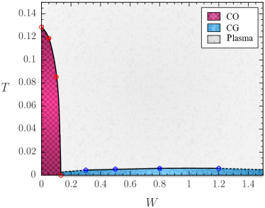
Figure 1: Phase diagram of the three-dimensional Coulomb glass model. There is a charge order (CO) phase for $W\lesssim 0.131$ where electrons and holes form a checkerboard-like crystal. For $W\gtrsim 0.131$ the system undergoes a glassy transition into the Coulomb glass (CG) phase, albeit at considerably lower temperatures than in the CO phase. The dashed lines indicate extrapolations where numerical simulations are not available.

II Model

The CG model in three spatial dimensions is described by the Hamiltonian

$$\mathcal{H}=\frac{e^{2}}{2\kappa}\sum_{i\neq j}(n_{i}-\nu)\frac{1}{|\mathbf{r}_{ij}|}(n_{j}-\nu)+\sum_{i}{n_{i}\phi_{i}},$$ (1)

where $\kappa=4\pi\epsilon_{0}$, $n_{i}\in\{0,1\}$, and $\nu$ is the filling factor. The disorder $\phi_{i}$ is an on-site Gaussian random potential, i.e., $\mathcal{P}(\phi_{i})=\left(2\pi W^{2}\right)^{-1/2}\exp\left(-{\phi_{i}^{2}}/{2W^{2}}\right)$. At half filling ($\nu=1/2$) the CG model can conveniently be mapped to a long-range spin model via $s_{i}=(2n_{i}-1)$. The Hamiltonian can be made dimensionless by choosing the units such that $e^{2}/\kappa=1$ and $a=1$ in which $a$ is the lattice spacing. We thus simulate

$$\mathcal{H}=\frac{1}{8}\sum_{i\neq j}\frac{s_{i}s_{j}}{|\mathbf{r}_{ij}|}+\frac{1}{2}\sum_{i}{s_{i}\phi_{i}},$$ (2)

where $s_{i}\in\{\pm 1\}$ represent Ising spins.

III Simulation details

In order to reduce the finite-size effects we use periodic boundary conditions. Special care has to be taken to deal with the long-range interactions. We make infinitely many periodic copies of each spin in all spatial directions, such that each spin interacts with all other spins infinitely many times. We use the Ewald summation technique Ewald (1921); de Leeuw et al. (1980), such that the double summation in Eq. (2) can be written in the following way

$$\frac{1}{2}\sum_{i=1}^{N}\sum_{j=1}^{N}s_{i}s_{j}\left[f^{(1)}_{ij}+f^{(2)}_{ij}+f^{(3)}_{ij}+f^{(4)}_{ij}\right],$$ (3)

where the terms $f_{ij}$ are defined as

$$f^{(1)}_{ij}=\frac{1}{4}\sideset{}{{}^{\prime}}{\sum}_{\mathbf{n}}\frac{\textrm{erfc}\left(\alpha|\mathbf{r}_{ij}+\mathbf{n}L|\right)}{|\mathbf{r}_{ij}+\mathbf{n}L|},$$ (4)

$$f^{(2)}_{ij}=\frac{\pi}{N}\sum_{\mathbf{k}\neq{0}}\frac{\mathrm{e}^{-\mathbf{k}^{2}/4\alpha^{2}}}{\mathbf{k}^{2}}\cos(\mathbf{k}\mathbf{r}_{ij}),$$ (5)

$$f^{(3)}_{ij}=\frac{\pi}{3N}\mathbf{r}_{i}.\mathbf{r}_{j},$$ (6)

$$f_{ij}^{(4)}=-\frac{\alpha}{2\sqrt{\pi}}\delta_{ij}.$$ (7)

Here, erfc is the complimentary error function Abramowitz and Stegun (1964), $\alpha$ is a regularization parameter, and $\mathbf{k}={2\pi\mathbf{n}}/{L}$ is the reciprocal lattice momentum. The vector index $\mathbf{n}$ in Eq. (4) runs over the lattice copies in all spatial directions and the prime indicates that $\mathbf{n}=0$ is not taken into account in the sum when $i=j$. For numerical purposes, the real and reciprocal space summations, i.e., Eqs. (4) and (5), respectively, are bounded by $|\mathbf{r}_{ij}+\mathbf{n}L|<r_{c}$ and $k<{2\pi n_{c}}/{L}$. The parameters $\alpha$, $r_{c}$, and $n_{c}$ are tuned to ensure a stable convergence of the sum. We find that $2<\alpha<4$, $n_{c}\gtrsim{4L}$, and $r_{c}=L/2$ are sufficient for the above purpose.

We use population annealing Monte Carlo (PAMC) Hukushima and Iba (2003); Machta (2010); Wang et al. (2015); Amey and Machta (2018); Barzegar et al. (2018) to thermalize the system down to extremely low temperatures. In PAMC, similarly to simulated annealing (SA) Kirkpatrick et al. (1983), the system is equilibrated towards a target temperature starting from a high temperature following an annealing schedule. PAMC, however, outperforms SA by introducing many replicas of the same system and thermalizing them in parallel. Each replica is subjected to a series of Monte Carlo moves and the entire pool of replicas is resampled according to an appropriate Boltzmann weight. This ensures that the system is equilibrated according to the Gibbs distribution at each temperature. For the simulations we use particle-conserving dynamics to ensure that the lattice half filling is kept constant, together with a hybrid temperature schedule linear in $\beta$ and linear in $T$ Barzegar et al. (2018). We use the family entropy of population annealing Wang et al. (2015) as an equilibration criterion. Hard samples are re-simulated with a larger population size and number of sweeps until the equilibration criterion is met. Note that we have independently examined the accuracy of the results, as well as the quality of thermalization for system sizes up to $L=8$ using parallel tempering Monte Carlo Hukushima and Nemoto (1996). Both data from PAMC and parallel tempering Monte Carlo agree within error bars. We investigate the phase diagram of the CG model using fixed values of the disorder width, i.e., vertical cuts on the $W$–$T$ plane. Further details of the simulation parameters can be found in Tables 1 and 2 for the CO and CG phases, respectively.

Table 1: PAMC simulation parameters used for the finite-temperature simulations in the CO phase ($W\leq 0.131$). $L$ is the linear system size, $R_{0}$ is the initial population size, $M$ is the number of Metropolis sweeps, $T_{0}$ is the lowest temperature simulated, $N_{T}$ is the number of temperatures and $N_{\rm sa}$ is the number of disorder realizations. Note that the the values in the table vary slightly for different values of the disorder $W$.

$L$	$R_{0}$	$M$	$T_{0}$	$N_{T}$	$N_{\rm sa}$
$4$	$2\times{10^{4}}$	$10$	$0.05$	$401$	$5000$
$6$	$5\times 10^{4}$	$10$	$0.05$	$601$	$5000$
$8$	$1\times{10^{5}}$	$20$	$0.05$	$801$	$2000$
$10$	$2\times{10^{5}}$	$20$	$0.05$	$1001$	$1000$
$12$	$5\times 10^{5}$	$30$	$0.05$	$1201$	$500$

Table 2: PAMC simulation parameters used for the finite-temperature simulations in the CG phase ($W>0.131$). For details see the caption of Table 1. Note that the the values in the table vary slightly for different values of the disorder $W$.

$L$	$R_{0}$	$M$	$T_{0}$	$N_{T}$	$N_{\rm sa}$
$4$	$2\times{10^{4}}$	$20$	$0.004$	$401$	$100000$
$6$	$5\times 10^{4}$	$30$	$0.004$	$601$	$50000$
$8$	$1\times{10^{5}}$	$40$	$0.004$	$801$	$30000$
$10$	$2\times{10^{5}}$	$60$	$0.004$	$1001$	$20000$

IV Results

IV.1 Charge-ordered phase

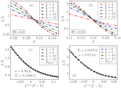
Figure 2: Finite-size correlation length per system size $\xi/L$ versus temperature $T$ for various disorder strengths. (a) No disorder, (b) small disorder ($W=0.05$). In both cases we observe a crossing of the data for different system sizes, suggesting a phase transition between a disordered electron plasma and a CO phase. (c), (d) Finite-size scaling analysis used to determine the best estimates for the critical temperature $T_{\rm c}$, as well as the critical exponent $\nu$ at the aforementioned disorder values. Note that the smallest system size is left out of the analysis for better accuracy. The transition temperature $T_{\rm c}$ of the CO phase decreases as the disorder grows.

To characterize the CO phase, we measure the specific heat capacity $c_{\rm v}=C_{\rm v}/N$ (only used to extract critical exponents, see Appendix B for details), staggered magnetization

$$m_{\rm s}=\frac{1}{N}\sum_{i=1}^{N}\sigma_{i},$$ (8)

where $\sigma_{i}=(-1)^{x_{i}+y_{i}+z_{i}}s_{i}$ and $N=L^{3}$ the number of spins, as well as the disconnected and connected susceptibility

$$\bar{\chi} =N[\langle m_{\rm s}^{2}\rangle],$$ (9)

$$\chi =N[\langle m_{\rm s}^{2}\rangle-\langle\left|m_{\rm s}\right|\rangle^{2}].$$ (10)

In addition, we measure the Binder ratio $g$ Binder (1981),

$$g=\frac{1}{2}\left(3-\frac{\left[\langle m_{\rm s}^{4}\rangle\right]}{\left[\langle m_{\rm s}^{2}\rangle\right]^{2}}\right),$$ (11)

and the finite-size correlation length $\xi/L$ Cooper et al. (1982); Palassini and Caracciolo (1999); Ballesteros et al. (2000), defined via

$$\xi=\frac{1}{2\sin\left(|\mathbf{k}_{\mathrm{min}}|/2\right)}\left(\frac{\chi(0)}{\chi(\mathbf{k}_{\mathrm{min}})}-1\right)^{1/2},$$ (12)

where $\mathbf{k}_{\mathrm{min}}=(2\pi/L,0,0)$ is the smallest nonzero wave vector and

$$\chi(\mathbf{k})=\frac{1}{N}\sum_{ij}[\langle\sigma_{i}\sigma_{j}\rangle]\exp(i\mathbf{k}.\mathbf{r}_{ij})$$ (13)

is the Fourier transform of the susceptibility. Furthermore, $\langle\cdots\rangle$ represents a thermal average and $[\cdots]$ is an average over disorder. According to the scaling ansatz, in the vicinity of a second-order phase transition temperature $T_{\rm c}$, any dimensionless thermodynamic quantity such as the Binder ratio and the finite-size correlation length divided by linear system size will be a universal function of $x=L^{1/\nu}(T-T_{\rm c})$, i.e., $g=\tilde{F}_{g}(x)$ and $\xi/L=\tilde{F}_{\xi}(x)$, where $\nu$ is a critical exponent. Therefore, an effective way of probing a phase transition is to search for a point where $g$ or $\xi/L$ data intersect. Given the universality of the scaling functions $\tilde{F}_{g}$ and $\tilde{F}_{\xi}$, if one plots $g$ or $\xi/L$ versus $x=L^{1/\nu}(T-T_{\rm c})$, the data for all system sizes must collapse onto a common curve. Because we are dealing with temperatures close to $T_{\rm c}$, we may approximate this universal curve by an appropriate mathematical function such as a third-order polynomial $f(x)=P_{3}(x)$ in the case of $\xi/L$ or a complimentary error function $f(x)=\frac{1}{2}{\rm erfc}(x)$ when studying the Binder cumulant. Hence, by fitting $f(x)$ to the data with $T_{\rm c}$ and $\nu$ as part of the fit parameters, we are able to determine their best estimates.

Table 3: Critical parameters of the plasma–CO phase transition at different disorder values. The exponents, except for $\nu$, change with disorder. Note that at $T=0$, the exponents $\alpha$ and $\gamma$ have been calculated in a different way (see text in Appendix B).

Model	$W$	$T_{\rm c}$	$\nu$	$\alpha/\nu$	$\beta/\nu$	$\bar{\gamma}/\nu$	$\gamma/\nu$
CG	$0.000$	$0.1284(1)$	$0.76(4)$	$0.550(2)$	$0.42(1)$	$2.41(1)$	$2.05(2)$
CG	$0.050$	$0.1187(3)$	$0.87(14)$	$0.418(25)$	$0.305(19)$	$2.67(2)$	$1.79(3)$
CG	$0.131(2)$	$0.000$	$0.71(5)$	$0.006(31)$	$0.154(5)$	$2.88(1)$	$1.55(4)$

The statistical error bars of the fit parameters are calculated by bootstrapping over the disorder realizations. In Fig. 2 we show the simulation data as well as the finite-size scaling (FSS) plots for $\xi/L$ at two different disorder values. Crossings can clearly be observed which signals a phase transition into the CO phase. Simulating multiple values of $W$, we observe a phase transition between a disordered electron plasma and a CO phase for $W<0.131(2)$, consistent with previous studies Malik and Kumar (2007); Pankov and Dobrosavljević (2005); Goethe and Palassini (2009). The CO phase is a checkerboard-like crystal Wigner (1934), where electrons and holes form a regular lattice as the potential energy dominates the kinetic energy at low temperatures.

We have also conducted zero-temperature simulations using simulated annealing to determine the zero-temperature critical disorder $W_{\rm c}$ that separates the CO from the CG phase. We average over $N_{\text{sa}}=2048$ different disorder realizations for disorders $W>0.10$ and $N_{\text{sa}}=512$ for $W\leq 0.10$. Each disorder realization is restarted at least at $20$ different initial random spin configurations and at each temperature step equilibrated $N_{\text{eq}}$ Monte Carlo steps. If at least $15\%$ of the runs reach the same minimal energy configuration, we assume that the chosen $N_{\text{eq}}$ was large enough and that the reached configuration is likely the ground state. If less than $15\%$ of the configurations reach the minimal state, we increase $N_{\text{eq}}$ and re-run the simulation until the $15\%$ threshold is achieved. For the largest simulated system size ($L=8$) and large disorders, typical equilibration times are $N_{\text{eq}}=2^{27}$ Monte Carlo sweeps.

To estimate $W_{\rm c}$, we use the Binder ratio defined in Eq. (11) which by definition quickly approaches $1$ when $T\rightarrow 0$ within the CO phase. Therefore, in order to retain a good resolution of a putative transition, we use an alternative quantity $\Gamma$ which is defined in the following way Möbius and Rössler (2009):

$$\Gamma=-\ln(1-g).$$ (14)

Close to $W_{\rm c}$, we may assume the following finite-size scaling behavior for $\Gamma$:

$$\Gamma=\tilde{F}_{\Gamma}\left[L^{1/\nu}(W-W_{\rm c})\right]$$ (15)

As $g$ is restricted to $0\leq g\leq 1$ with a step-function like shape, we may use a complimentary error function $\frac{1}{2}{\rm erfc}(\frac{x-\mu}{\sigma})$ to represent the universal scaling function $\tilde{F}_{\Gamma}$ in which $x=L^{1/\nu}(W-W_{\rm c})$ and $W_{\rm c}$, $\nu$, $\mu$, $\sigma$ are the fit parameters. The fit is shown in Fig. 3 where we obtain $W_{\rm c}=0.131\pm 0.002$ and $\nu=0.71\pm 0.05$. In Table 3 (Appendix B) we list the values of the critical exponents for the plasma–CO phase transition for various disorder values $W$ after a comprehensive FSS analysis of different observables. Note that we have used the methods developed in Ref. Hartmann and Young (2001) to compute the exponents $\alpha$ and $\gamma$ at $T\!=\!0$. An important observation one can promptly make is that the exponents—except for $\nu$ which is universal—vary with disorder. This can be attributed to the fact that the perturbations at large length scales are contested between random field fluctuations which have static nature and dynamic thermal fluctuations Grinstein (1976); Bray and Moore (1985); Fisher (1986). At $W\!=0$, the perturbations are purely thermal, while at $T\!=\!0$, the random field completely dominates. At such large length scales, the interactions within the charge ordered phase resemble the random-field Ising model (RFIM) Middleton and Fisher (2002); Fytas and Martin-Mayor (2013); Fytas et al. (2013); Ahrens et al. (2013) with short-range bonds, namely, screening takes place. This can be understood by remembering that the dynamics of the system is constrained by charge conservation. In the spin language, excitations are no longer spin flips but spin-pair flip-flops owing to the conservation of total magnetization. For instance, one can create a local excitation while preserving charge neutrality by moving a number of electrons out of a subdomain in the CO phase. The excess energy of such a domain scales like its surface, similarly to the short-range ferromagnetic Ising model. It is worth mentioning that the Imry-Ma Imry and Ma (1975) picture gives a lower critical dimension of $2$ for discrete spins with short-range interactions. Hence three-dimensional Ising spins, such as in the RFIM, are stable to small random fields as we also find here.

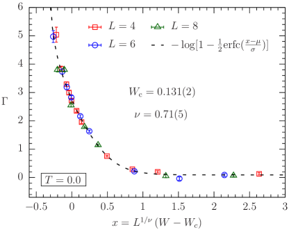
Figure 3: Zero-temperature simulation results for the plasma–CO phase transition. The quantity $\Gamma$ defined in Eq. (14) is used to perform a finite-size scaling analysis. We conclude that the CO phase terminates at $W_{c}=0.131(2)$. The statistical error bars are estimates by bootstrapping over disorder instances. ${\rm erfc}(x)$ is the complimentary error function which is used to fit the Binder ratio data (see text).

Returning to the discussion of the critical exponents, we note that scaling relations such as

$$\gamma=\beta(\delta-1)=(2-\eta)\nu,$$ (16)

as well as the modified hyperscaling relation

$$(d-\theta)\nu=2-\alpha=2\beta+\gamma$$ (17)

can be utilized to obtain estimates for the critical exponents $\eta$, $\theta$, and $\delta$. For instance, using the values in Table 3, we see that $\eta(W=0.0)=-0.05(2)$ and $\eta(W=0.05)=0.22(1)$. Near criticality, the correlation functions decay as a power of distance, i.e., $G(\mathbf{x})\sim 1/|\mathbf{x}|^{d-2+\eta}$. The fact that the exponent $\eta$ is slightly negative for $W=0.0$ shows that correlation between the spins remains in effect over a much longer distance in the absence of disorder. Physically this is plausible, as disorder tends to decorrelate the spins.

IV.2 Coulomb glass phase

To examine the existence of a glassy phase in the CG model, we measure the spin-glass correlation length defined in Eq. (12), however, for a spin-glass order parameter, namely

$$\xi_{\rm SG}=\frac{1}{2\sin\left(|\mathbf{k}_{\mathrm{min}}|/2\right)}\left(\frac{\chi_{\rm SG}(0)}{\chi_{\rm SG}(\mathbf{k}_{\mathrm{min}})}-1\right)^{1/2}.$$ (18)

Here, the spin-glass susceptibility $\chi_{\rm SG}$ has the following definition Ballesteros et al. (2000):

$$\chi_{\rm SG}(\mathbf{k})=\frac{1}{N}\sum_{i=1}^{N}\sum_{j=1}^{N}\left[\left(\langle s_{i}s_{j}\rangle\!-\!\langle s_{i}\rangle\langle s_{i}\rangle\right)^{2}\right]\!\mathrm{e}^{i\mathbf{k}.(\mathbf{r}_{i}-\mathbf{r}_{j})}.$$ (19)

It is important to note that $\langle s_{i}\rangle\neq 0$ because the Hamiltonian [Eq. (2)] is not symmetric under global spin flips. Therefore, at least four replicas are needed to compute the connected correlation function in Eq. (19). We start with the partition function of the system, using Eq. (2):

$$Z=\sum_{\{s_{i}\}}\exp\left[-\beta\left(\frac{1}{8}\sum_{i\neq j}\frac{s_{i}s_{j}}{|\mathbf{r}_{ij}|}+\frac{1}{2}\sum_{i}{s_{i}\phi_{i}}\right)\right].$$ (20)

We may now expresses any combination of the spin moments in terms of the replicated spin variables $s_{i}^{\alpha}$ in the following way

$$\langle s_{1_{1}}\ldots s_{1_{k_{1}}}\rangle^{l_{1}}\dots\langle s_{m_{1}}\ldots s_{m_{k_{m}}}\rangle^{l_{m}}$$

$$=\,\frac{1}{Z^{n}}\sum_{\{s_{i}^{\alpha}\}}\mathrm{e}^{-\beta\!\!\sum\limits_{\alpha=1}^{n}\!\!\mathcal{H}[\{s_{i}^{\alpha}\}]}s_{1_{1}}^{1}\ldots s_{1_{k_{1}}}^{1}\cdots\,s_{m_{1}}^{n}\ldots s_{m_{k_{m}}}^{n}$$

$$=\,\frac{1}{n!}\sum_{\alpha_{1}\ldots\alpha_{n}}^{n}\langle s_{1_{1}}^{\alpha_{1}}\ldots s_{1_{k_{1}}}^{\alpha_{1}}\cdots\,s_{m_{1}}^{\alpha_{n}}\ldots s_{m_{k_{m}}}^{\alpha_{n}}\rangle,$$ (21)

where $n=l_{1}+\cdots+l_{m}$ is the total number of replicas and replica indices $\alpha_{1}$, $\ldots$ $\alpha_{n}$ are all distinct. As a special case, one can show

$$\left(\langle s_{i}s_{j}\rangle-\langle s_{i}\rangle\langle s_{j}\rangle\right)^{2}= \,\frac{2}{4!}\sum_{\alpha,\beta}^{4}\langle s_{i}^{\alpha}s_{j}^{\alpha}s_{i}^{\beta}s_{j}^{\beta}\rangle$$

$$-\frac{2}{4!}\sum_{\alpha,\beta,\gamma}^{4}\langle s_{i}^{\alpha}s_{j}^{\alpha}s_{i}^{\beta}s_{j}^{\gamma}\rangle$$

$$+\frac{1}{4!}\sum_{\alpha,\beta,\gamma,\lambda}^{4}\langle s_{i}^{\alpha}s_{i}^{\beta}s_{j}^{\gamma}s_{j}^{\lambda}\rangle.$$ (22)

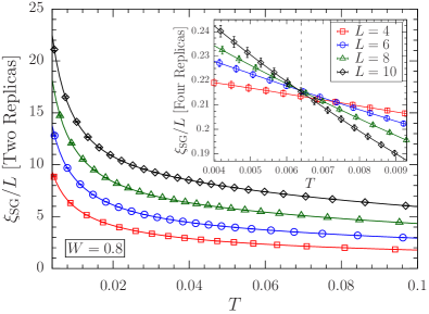
Figure 4: Spin-glass correlation length divided by system size $\xi_{\rm SG}/L$ calculated using two replicas at $W=0.8$ versus temperature $T$. No crossing is observed down to very low temperatures. The inset shows the same quantity using four replicas where a transition is clearly visible. Here, data points for different system sizes cross approximately at the temperature indicated by the dashed line. This suggests that in the presence of external fields four-replica quantities need to be used to characterize phase transitions in glassy systems.

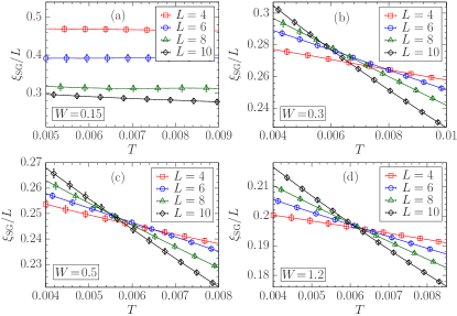
Figure 5: Spin-glass finite-size correlation length $\xi_{\rm SG}/L$ as a function of temperature $T$ at various disorder strengths $W$. (a) $W=0.15$, (b) $W=0.30$, (c) $W=0.50$, and (d) $W=1.20$. For $W\gtrsim 0.15$ the data for different system sizes cross, indicating a plasma–CG phase transition. Corrections to scaling must be considered to reliably estimate the value of the critical temperature $T_{\rm c}$ (see text for details).

Using the above expression, the spin-glass susceptibility [Eq. (19)] can be written in terms of the replica overlaps as follows:

$$\chi_{\rm SG}(\mathbf{k})= \,\frac{N}{6}\sum_{\alpha<\beta}^{4}\left[\langle q_{\alpha\beta}(\mathbf{k})q^{*}_{\alpha\beta}(\mathbf{k})\rangle\right]$$

$$-\frac{N}{6}\sum_{\alpha}^{4}\sum_{\beta<\gamma}^{4}\left[\langle q_{\alpha\beta}(\mathbf{k})q^{*}_{\alpha\gamma}(\mathbf{k})\rangle\right]$$

$$+\frac{N}{3}\sum_{\alpha<\beta}^{4}\sum_{\gamma<\lambda}^{4}\left[\langle q_{\alpha\beta}(\mathbf{k})q^{*}_{\gamma\lambda}(\mathbf{k})\rangle\right].$$ (23)

Once again, the indices $\alpha$, $\beta$, $\gamma$, and $\lambda$ must be distinct. Here, $q^{*}_{\alpha\beta}(\mathbf{k})$ represents the complex conjugate of $q_{\alpha\beta}(\mathbf{k})$, and $q_{\alpha\beta}(\mathbf{k})$ is the Fourier transformed spin overlap, i.e.,

$$q_{\alpha\beta}(\mathbf{k})=\frac{1}{N}\sum_{i=1}^{N}s_{i}^{\alpha}s_{i}^{\beta}\mathrm{e}^{i\mathbf{k}.\mathbf{r}_{i}}.$$ (24)

To underline the significance of this matter, we have shown in Fig. 4 the spin-glass correlation length calculated using two replicas, as has been done in some previous numerical studies of the CG Grannan and Yu (1993); Bhandari and Malik (2019). The inset shows the same quantity computed using four replicas. While the two-replica version of the finite-size correlation length shows no sign of a CG transition, the four-replica expression captures the existence of a phase transition into a glassy phase.

We have performed equilibrium simulations for $W\in\{0.15,0.30,0.50,0.80,1.2\}$. In Fig. 5 we plot the four-replica spin-glass correlation length as a function of temperature at selected disorder values. Our results strongly suggest that there is a transition to a glassy phase which persists for relatively large values of the disorder. This is significant in the sense that it confirms the phase transition via replica symmetry breaking as predicted by mean-field theory. The nontriviality of our findings can be better understood if one juxtaposes the CG case with that of finite-dimensional spin glasses lacking time reversal symmetry due to an arbitrarily small external field where the existence of de Almeida-Thouless de Almeida and Thouless (1978) transition, except for a few rare cases Baños et al. (2012); Baity-Jesi et al. (2014), has been ruled out by numerous studies Fisher and Huse (1987, 1988); Mattsson et al. (1995); Jönsson et al. (2005); Takayama and Hukushima (2004); Young and Katzgraber (2004). For the random-field Ising model the droplet picture of Fisher and Huse Fisher and Huse (1987, 1988) can be invoked to show the instability of the glass phase to infinitesimal random fields. Yet, the CG model is different in two significant ways: typical compact domains are not charge neutral, and therefore can not be flipped; and the long range of the interactions, while it does not affect the domain wall formation energy in the ordered phase, may be significant in the more complex domain formation of the glass phase. It is worth emphasizing here that proper equilibration is key in observing a glassy phase in the CG simulations. For instance, in Fig. 8 of Appendix A we show an example of a simulation where the crossing in the spin-glass correlation length is completely masked due to insufficient thermalization.

Some corrections to scaling must be considered in the analysis in order to estimate the position of the critical temperature and the values of the critical exponents. In the vicinity of the critical temperature $T_{\rm c}$ and to leading order in corrections to scaling, we may consider the following FSS expressions for the spin-glass susceptibility $\chi_{\rm SG}$ and the finite-size two-point correlation length divided by the linear size of the system, $\xi_{\rm SG}/L$:

$$\chi_{\rm SG}\sim C_{\chi}L^{2-\eta}\left[1+A_{\chi}L^{-\omega}+B_{\chi}L^{1/\nu}(T-T_{\rm c})\right],$$ (25)

$$\xi_{\rm SG}/L\sim C_{\xi}+A_{\xi}L^{-\omega}+B_{\xi}L^{1/\nu}(T-T_{\rm c}),$$ (26)

where $A_{\chi}$, $B_{\chi}$, $C_{\chi}$, $A_{\xi}$, $B_{\xi}$, and $C_{\xi}$ are constants. In order to find the critical temperature $T_{\rm c}$ as well as the critical exponents $\nu$, $\eta$, $\omega$, we perform the following procedure.

1. Estimation of $T_{\rm c}$: Given any pair of system sizes $(L_{1},L_{2})$ we have

   $$L_{1}=\bar{L}-\Delta L/2,\quad L_{2}=\bar{L}+\Delta L/2,$$ (27)

   in which $\Delta L=L_{2}-L_{1}$ and $\bar{L}=(L_{1}+L_{2})/2$. Using Eq. (26), to the leading order in $\Delta L/\bar{L}$ we find

   $$\frac{\xi_{\rm SG}(L_{i},T)}{L_{i}}\sim\frac{\xi_{\rm SG}(\bar{L},T)}{\bar{L}}-(-1)^{i}\frac{\Delta L}{2\bar{L}}\left[\omega A_{\xi}\bar{L}^{-\omega}\right.$$

   $$\left.-\frac{B_{\xi}}{\nu}\bar{L}^{1/\nu}(T-T_{\rm c})\right],$$ (28)

   where the index $i$ can take values $i=1,2$. One can now use Eq. (28) to determine the temperature $T^{*}(L_{1},L_{2})$ at which the curves of $\xi_{\rm SG}/L$ cross; in other words, $\xi_{\rm SG}(L_{1},T^{*})/L_{1}=\xi_{\rm SG}(L_{2},T^{*})/L_{2}$ and

   $$T^{*}(L_{1},L_{2})\sim T_{\rm c}+\Theta_{\xi}\bar{L}^{-\omega-1/\nu}=T_{\rm c}+\Theta_{\xi}\bar{L}^{-\phi}.$$ (29)

   Here $T_{\rm c}$ is the true critical temperature in the limit $L\rightarrow\infty$ and $\Theta_{\xi}$ is a constant. In Fig. 6(a), we show the $T_{\rm c}$ estimate for the case $W=0.50$. The best fit curve is obtained by minimizing the sum of the square of the residuals,

   $$\chi^{2}=\sum_{i=1}^{N}\left(T_{i}^{*}-T_{\rm c}-\Theta_{\xi}\bar{L}_{i}^{-\phi}\right)^{2},$$ (30)

   where $i$ runs over all pairs of linear system sizes. Now we vary $T_{\rm c}$, minimizing $\chi^{2}$ along the way with respect to the remaining parameters. Since $\Theta_{\xi}$ appears linearly in the model, it can be eliminated Lawton and Sylvestre (1971) to reduce the optimization task to one free parameter, i.e., $\phi$:

   $$\left(\frac{\partial\chi^{2}}{\partial\Theta_{\xi}}\right)_{T_{\rm c}}\!\!\!=0\,\,\Rightarrow\,\,\tilde{\Theta}_{\xi}(T_{\rm c},\phi)=\frac{\sum\limits_{i=1}^{N}(T^{*}_{i}-T_{\rm c})\bar{L}_{i}^{-\phi}}{\sum\limits_{i=1}^{N}\bar{L}_{i}^{-2\phi}}.$$ (31)

   Because there are five data points with three parameters in the original model, we have two degrees of freedom. Therefore, the probability density function (PDF) is proportional to $e^{-\chi^{2}/2}$.

   

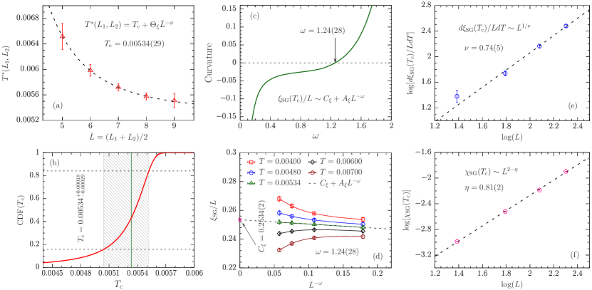
   Figure 6: Process of estimating the critical exponents, as well as the critical temperature $T_{\rm c}$ of the plasma–CG phase transition for $W=0.5$. Other values of $W$ are analyzed using the same procedure. (a) The temperatures where $\xi_{\rm SG}/L$ curves of different systems sizes cross are used to determine the critical temperature $T_{\rm c}$. The crossing temperatures decay toward the thermodynamic limit $T_{\rm c}$. (b) The cumulative distribution function (CDF) is constructed by minimizing $\chi^{2}$ with respect to $\Theta_{\xi}$ and $\phi$ while holding $T_{\rm c}$ constant. The shaded region shows the $68\%$ confidence interval and the green vertical line indicates the best estimate of $T_{\rm c}$. (c) The value of $T_{\rm c}$ obtained in the previous step is used to determine $\omega$. At $T=T_{\rm c}$ and optimal $\omega$, $\xi_{\rm SG}/L$ is linear as a functions of $L^{-\omega}$; i.e., it has zero curvature as demonstrated in panel (d). (e) The critical exponent $\nu$ is estimated using the derivative of $\xi_{\rm SG}/L$ with respect to temperature which scales as $L^{1/\nu}$ when evaluated at $T_{\rm c}$. Some deviations are evident for the smallest system size. (f) The spin-glass susceptibility $\chi_{\rm SG}$ at $T=T_{\rm c}$ which scales as $L^{2-\eta}$ is used to determine the best estimate of the exponent $\eta$.

   To determine the confidence intervals, we calculate the cumulative distribution function (CDF) Katzgraber and Young (2003):

   $$Q(T_{\rm c})=\int^{T_{\rm c}}e^{-\frac{1}{2}\chi^{2}(T^{\prime}_{\rm c})}dT^{\prime}_{\rm c}.$$ (32)

   As an example, in Fig. 6(b) we have shown the $68\%$ confidence interval as well as the best estimate for the critical temperature.

2. Estimation of $\omega$: From Eq. (26) we observe that

   $$\xi_{\rm SG}(T_{\rm c})/L\sim C_{\xi}+A_{\xi}L^{-\omega}.$$ (33)

   Table 4: Critical parameters of the plasma–CG phase transition for various values of the disorder $W$. The exponent $\nu$ and $\omega$ are independent of $W$ within error bars highlighting their universality whereas the exponent $\eta$ varies as the disorder strength increases.

   $W$	$T_{\rm c}$	$\nu$	$\omega$	$\eta$
   $0.300$	$0.00446(25)$	$0.62(5)$	$1.26(7)$	$0.56(1)$
   $0.500$	$0.00534(29)$	$0.74(5)$	$1.24(28)$	$0.82(5)$
   $0.800$	$0.00590(56)$	$0.64(2)$	$1.28(20)$	$0.97(5)$
   $1.200$	$0.00600(16)$	$0.65(3)$	$1.33(21)$	$1.09(1)$

   Thus, using the best estimate of $T_{\rm c}$ from the previous step, we expect the data points of $\xi_{\rm SG}(T_{\rm c})/L$ as a function of $L^{-\omega}$ to follow a straight line when $\omega$ is chosen correctly. We can therefore vary $\omega$ and measure the curvature until it vanishes at the optimal value. We have demonstrated this in Figs. 6(c) and 6(d). Note that the error bar for $\omega$ is calculated using the bootstrap method.

3. Estimation of $\nu$ and $\eta$: It is straightforward to show from Eqs. (25) and (26) that to the leading order in corrections,

   $$\chi_{\rm SG}(T_{\rm c})=C_{\chi}L^{2-\eta}(1+A_{\chi}L^{-\omega}),$$ (34)

   $$\frac{d}{dT}(\xi_{\rm SG}/L)(T_{\rm c})=B_{\xi}L^{1/\nu}(1+D_{\xi}L^{-\omega}),$$ (35)

   in which the best estimates obtained for $T_{\rm c}$ and $\omega$ are used. We see that the above quantities simply scale as $\chi_{\rm SG}(T_{\rm c})\sim L^{2-\eta}$ and $\frac{d}{dT}(\xi_{\rm SG}/L)(T_{\rm c})\sim L^{1/\nu}$ for large enough $L$. Therefore, a linear fit in logarithmic scale will yield the exponents $\nu$ and $\omega$. This is shown in Figs. 6(e) and 6(f), respectively.

   The above procedure has been repeated for all other values of the disorder $W$. The results are summarized in Table 4 of Appendix B. We observe that within the error bars, the critical exponents $\nu$ and $\omega$ are robust to disorder which underlines the universality of these exponents. Nevertheless, larger system sizes—currently not accessible via simulation—would be needed to conclusively determine the universality class of the model. The fact that we observe stronger corrections to scaling for smaller disorder shows that the energy landscape is rougher due to competing interactions where finite-size effects are accentuated. For larger values of $W$, on the other hand, the system becomes easier to thermalize as the disorder dominates the electrostatic interactions.

V Conclusion

We have shown that, using the four-replica expressions for the commonly-used observables, the CG model displays a transition into a glassy phase for the studied system sizes, provided that large enough disorder and sufficiently low temperatures are used in the simulations (see Fig. 1 for the complete phase diagram of the model). Previous numerical studies—including a work Surer et al. (2009) by a subset of us—have failed to observe the glassy phase. In this study, we are able to present strong numerical evidence for the validity of the mean-field results in three space dimensions, which predicts transition to a glassy phase at large disorder via replica symmetry breaking. Moreover, we corroborate the results of previous studies for the low-disorder regime where a CO phase, similar to the ferromagnetic phase in the RFIM, is observed. Interestingly, for large disorder values, the CG and the RFIM are different, as the RFIM does not exhibit a transition into a glassy phase (see, for example, Ref. Ahrens et al. (2013) and references therein). A possible reason is the combination of the constrained dynamics (magnetization-conserving dynamics) and the long-range Coulomb interactions not present in the RFIM. These two factors can increase frustration such that a glassy phase can emerge. Our findings open the possibility of describing electron glasses through an effective CG model both theoretically and numerically. Because most of the electron glass experiments are performed in two-dimensional materials, it would be desirable to investigate these results in two-dimensional models. Our preliminary results in two space dimensions show no sign of a glass phase.

Appendix A Equilibration

In this appendix, we outline the steps taken to guarantee thermalization. The data for this work are predominantly generated using population annealing Monte Carlo (PAMC). In order to ensure that the states sampled by a Monte Carlo simulation are in fact in thermodynamic equilibrium, i.e., weighted according to the Boltzmann distribution, one needs to strive against bias by controlling the systematic errors intrinsic to the algorithm due to the finite population size.

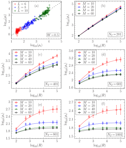
Figure 7: Equilibration of a PAMC simulation. (a) Equilibration population size $\rho_{\rm f}$ versus entropic family size $\rho_{\rm s}$ for a CG simulations at $W=0.5$. $100$ instances for each system size have been studied. Evidently, $\rho_{\rm s}$ is greatly correlated to $\rho_{\rm f}$ which controls the systematic errors in thermodynamic quantities. Because $\rho_{\rm f}$ is computationally expensive to measure, one may instead use $\rho_{\rm s}$ as the measure of thermalization. (b)–(f) $\rho_{\rm s}$ versus the population size $R$ for system size $L=8$ at various number of temperatures $N_{T}$ and Metropolis sweeps $M$. When $\rho_{\rm s}$ converges, the system is guaranteed to be in thermal equilibrium. As seen from the plots, convergence is achieved faster as the number of temperatures and sweeps is increased. However, for extremely large values of $N_{T}$ and $M$, marginal improvement in equilibration is gained at the cost of extended run time of the simulation.

Fortunately, PAMC offers a convenient way to study and tune the systematic errors to a desired accuracy. It can be shown Wang et al. (2015) that the systematic errors in a PAMC simulation are directly proportional to the equilibration population size $\rho_{\rm f}$ which has the following definition:

$$\rho_{\rm f}=\lim_{R\rightarrow\infty}\!R\,{\rm var}(\beta F).$$ (36)

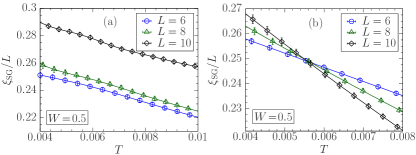
Figure 8: Importance of proper thermalization in observing a CG phase transition. Panel (a) shows a simulation where some instances have not reached thermal equilibrium whereas panel (b) illustrates the same simulation in which all of the instances have been thoroughly thermalized.

Here, $R$ is the population size and $F$ is the free energy. $\rho_{\rm f}$ is an extensive quantity defined at the thermodynamic limit although in reality it converges at a large but finite $R$. Because $\rho_{\rm f}$ is computationally expensive to measure as it requires multiple independent runs, one may alternatively study the entropic family size $\rho_{\rm s}$ defined as

$$\rho_{\rm s}=\lim_{R\rightarrow\infty}\!R\,e^{-S_{\rm f}},$$ (37)

where $S_{\rm f}$ is the family entropy of PAMC. As shown in of Fig. 7(a), $\rho_{\rm s}$ is well correlated with $\rho_{\rm f}$ which is why we can reliably use $\rho_{\rm s}$ as the measure of equilibration. $\rho_{\rm s}$ similarly to $\rho_{\rm f}$ converges at a finite $R$. The population size at which the convergence is achieved is a function of the number of temperatures $N_{T}$ as well as the number of Metropolis sweeps $M$. Optimization of PAMC is studied in great detail in the context of spin glasses Barzegar et al. (2018); Amey and Machta (2018) much of which can be carried over to the CG simulations. As an example we show in Figs. 7(b)–7(f) how we choose the optimal values of the PAMC parameters. We observe that the convergence of $\rho_{\rm s}$ is attained faster as the number of temperatures and sweeps is increased. However, beyond a certain point, any further increase solely prolongs the simulation time while contributing negligibly to lowering the convergent value of $\rho_{\rm s}$. A good rule of thumb for checking thermalization, as seen in Fig. 7, is that $\rho_{\rm s}$ and as a result $\rho_{\rm f}$ converges when $\rho_{\rm s}/R=\exp({-S_{\rm f}})<0.01$. We ensure that the above criterion is met for every instance that we have studied. This matter has been investigated thoroughly in Ref. Wang et al. (2015). It is worth mentioning here that proper equilibration is crucial in observing phase transitions, especially in subtle cases like the CG model. We have illustrated this matter in Fig. 8. Figure 8(a) shows a simulation where the system has been poorly thermalized in which $\rho_{\rm s}/R\sim 0.1$ on average across the studied instances. By contrast in Fig. 8(b) the same simulation is done with careful equilibration; that is to say, the criterion $\rho_{\rm s}/R<0.01$ is strictly enforced for every instance. It is clear that the observation of a crossing is contingent upon ensuring that every instance has reached thermal equilibrium. This, in turn, could explain why simulations using parallel tempering Monte Carlo, e.g., Ref. Goethe and Palassini (2009), see no sign of a transition.

Appendix B Finite-size scaling results

Figure 9: Finite-size scaling analysis for the plasma–CO phase transition at $W\!=\!0.05$. The peak values of the specific heat capacity $c_{\rm v}$, connected and disconnected susceptibilities $\chi$ and $\bar{\chi}$, as well as the inflection point value of the staggered magnetization are used to estimate the critical exponents $\alpha$, $\beta$, $\gamma$, and $\bar{\gamma}$, respectively. According to Eqs. (39) and (40), the above quantities scale as a power law in the linear system size $L$ as clearly seen from the figure.

In this appendix we list the estimates for the critical parameters of the plasma–CO, as well as the plasma–CG phase transitions. Because the CO phase is essentially an antiferromagnetic phase in the spin language, multiple critical exponents such as $\nu$, $\alpha$, $\beta$, and $\gamma$ can be measured numerically. We have estimated these quantities using FSS techniques, specifically by a FSS collapse of the data for different system sizes onto a low-order polynomial, as explained in the main text. To estimate the exponent $\nu$ we have used the finite-size correlation length per linear system size $\xi/L$ [Eq. (12)]. Because this is a dimensionless quantity, in the vicinity of the critical point it scales as

$$\xi/L ={F}_{\xi}\left[L^{1/\nu}(T-T_{\rm c})\right].$$ (38)

Other critical exponents such as $\alpha$, $\gamma$, and $\beta$ can be estimated by performing a FSS analysis using the peak values of the specific heat $c_{\rm v}=C_{\rm v}/N$, connected susceptibility $\chi$, and the disconnected susceptibility $\bar{\chi}$ as well as the inflection point value of the staggered magnetization $m_{\rm s}$ which scale as following:

$$c_{\rm v}^{\rm max}\sim L^{\alpha/\nu},\quad m_{\rm s}^{\rm inflect}\sim L^{-\beta/\nu}.$$ (39)

$$\chi^{\rm max}\sim L^{\gamma/\nu},\quad\bar{\chi}^{\rm max}\sim L^{\bar{\gamma}/\nu}.$$ (40)

As we can see in Fig. 9 the above scaling behaviors are very well satisfied. The best estimates of the critical parameters for various values of the disorder are listed in Table 3. Note that with the exception of the universal exponent $\nu$, other critical exponents vary with disorder which can be due to the trade-off between large-scale thermal and random-field fluctuations. Because at $T\!=\!0$ the system has settled in the ground state, one cannot use thermal sampling to measure the variance of energy and staggered magnetization which are proportional to the heat capacity and susceptibility, respectively. Instead, we have used the techniques developed by Hartmann and Young in Ref. Hartmann and Young (2001).

For the plasma–CG transition we have calculated the critical exponents $\nu$ and $\eta$, as well as the correction to scaling exponent $\omega$, using the procedure explained in Sec. IV.2. Table  4 lists the estimates of the critical parameters. Within the error bars, the exponents $\nu$ and $\omega$ are independent of disorder, whereas $\eta$ changes as the disorder strength increases.

References

- Anderson (1958) P. W. Anderson, Absence of Diffusion in Certain Random Lattices, Phys. Rev. 109, 1492 (1958).
- Pollak (1970) M. Pollak, Disc. Faraday Soc. 50, 13 (1970).
- Srinivasan (1971) G. Srinivasan, Statistical Mechanics of Charged Traps in an Amorphous Semiconductor, Phys. Rev. B 4, 2581 (1971).
- Efros and Shklovskii (1975) A. L. Efros and B. I. Shklovskii, Coulomb gap and low temperature conductivity of disordered systems , J. Phys. C 8, L49 (1975).
- Grünewald et al. (1982) M. Grünewald, B. Pohlmann, L. Schweitzer, and D. Würtz, Mean field approach to the electron glass, J. Phys. C 15, 1153 (1982).
- Pollak (1975) M. Pollak, The Coulomb gap: a Review and New Developments, Phil. Mag. B 65, 657 (1975).
- Vojta (1993) T. Vojta, Spherical random-field systems with long-range interactions: general results and application to the Coulomb glass, J. Phys. A 26, 2883 (1993).
- Pastor and Dobrosavljević (1999) A. A. Pastor and V. Dobrosavljević , Melting of the Electron Glass, Phys. Rev. Lett. 83, 4642 (1999).
- Pastor et al. (2002) A. A. Pastor, V. Dobrosavljević, and M. L. Horbach, Mean-field glassy phase of the random-field Ising model, Phys. Rev. B 66, 014413 (2002).
- Dobrosavljević et al. (2003) V. Dobrosavljević, D. Tanasković, and A. A. Pastor, Glassy Behavior of Electrons Near Metal-Insulator Transitions, Phys. Rev. Lett. 90, 016402 (2003).
- Müller and Ioffe (2004) M. Müller and L. B. Ioffe, Glass Transition and the Coulomb Gap in Electron Glasses, Phys. Rev. Lett. 93, 256403 (2004).
- Pankov and Dobrosavljević (2005) S. Pankov and V. Dobrosavljević, Nonlinear Screening Theory of the Coulomb Glass, Phys. Rev. Lett. 94, 046402 (2005).
- Lebanon and Müller (2005) E. Lebanon and M. Müller, Memory effect in electron glasses: Theoretical analysis via a percolation approach, Phys. Rev. B 72, 174202 (2005).
- Amir et al. (2008) A. Amir, Y. Oreg, and Y. Imry, Mean-field model for electron-glass dynamics, Phys. Rev. B 77, 165207 (2008).
- Monroe et al. (1987) D. Monroe, A. C. Gossard, G. B. English, J. H., W. H. Haemmerle, and M. Kastner, Long Lived Coulomb Gap in a Compensated Semiconductor - The Electron Glass, Phys. Rev. Lett. 59, 1148 (1987).
- Ben-Chorin et al. (1993) M. Ben-Chorin, Z. Ovadyahu, and M. Pollak, Nonequilibrium transport and slow relaxation in hopping conductivity, Phys. Rev. B 48, 15025 (1993).
- Massey and Lee (1995) J. G. Massey and M. Lee, Direct Observation of the Coulomb Correlation Gap in a Nonmetallic Semiconductor, Si:B, Phys. Rev. Lett. 75, 4266 (1995).
- Ovadyahu and Pollak (1997) Z. Ovadyahu and M. Pollak, Disorder and Magnetic Field Dependence of Slow Electronic Relaxation, Phys. Rev. Lett. 79, 459 (1997).
- Martinez-Arizala et al. (1998) G. Martinez-Arizala, C. Christiansen, D. E. Grupp, N. Markovic, A. M. Mack, and A. M. Goldman, Coulomb-glass-like behavior of ultrathin films of metals, Phys. Rev. B 57, R670 (1998).
- Vaknin et al. (2000) A. Vaknin, Z. Ovadyahu, and M. Pollak, Aging Effects in an Anderson Insulator, Phys. Rev. Lett. 84, 3402 (2000).
- Bogdanovich and Popovic (2002) S. Bogdanovich and D. Popovic, Onset of Glassy Dynamics in a Two-Dimensional Electron System in Silicon, Phys. Rev. Lett. 88, 236401 (2002).
- Vaknin et al. (2002) A. Vaknin, Z. Ovadyahu, and M. Pollak, Nonequilibrium field effect and memory in the electron glass, Phys. Rev. B 65, 134208 (2002).
- Orlyanchik and Ovadyahu (2004) V. Orlyanchik and Z. Ovadyahu, Stress Aging in the Electron Glass, Phys. Rev. Lett. 92, 066801 (2004).
- Romero and Drndic (2005) H. E. Romero and M. Drndic, Coulomb Blockade and Hopping Conduction in PbSe Quantum Dots, Phys. Rev. Lett. 95, 156801 (2005).
- Jaroszyński and Popović (2006) J. Jaroszyński and D. Popović, Nonexponential Relaxations in a Two-Dimensional Electron System in Silicon, Phys. Rev. Lett. 96, 037403 (2006).
- Grenet et al. (2007) T. Grenet, J. Delahaye, M. Sabra, and F. Gay, Anomalous electric-field effect and glassy behaviour in granular aluminium thin films: electron glass?, Euro. Phys. J. B 56, 183 (2007).
- Ovadyahu (2007) Z. Ovadyahu, Relaxation Dynamics in Quantum Electron Glasses, Phys. Rev. Lett. 99, 226603 (2007).
- Raičević et al. (2008) I. Raičević, J. Jaroszyński, D. Popović, C. Panagopoulos, and T. Sasagawa, Evidence for Charge Glasslike Behavior in Lightly Doped La2-xSrxCuO4 at Low Temperatures, Phys. Rev. Lett. 101, 177004 (2008).
- Raičević et al. (2011) I. Raičević, D. Popović, C. Panagopoulos, and T. Sasagawa, Non-Gaussian noise in the in-plane transport of lightly doped La2-xSrxCuO4: Evidence for a collective state of charge clusters, Phys. Rev. B 83, 195133 (2011).
- Müller and Pankov (2007) M. Müller and S. Pankov, Mean-field theory for the three-dimensional Coulomb glass, Phys. Rev. B 75, 144201 (2007).
- Grannan and Yu (1993) E. R. Grannan and C. C. Yu, Critical behavior of the Coulomb glass, Phys. Rev. Lett. 71, 3335 (1993).
- Vojta and Schreiber (1994) T. Vojta and M. Schreiber, Comment on “Critical behavior of the Coulomb glass”, Phys. Rev. Lett. 73, 2933 (1994).
- Baranovskii et al. (1979) S. D. Baranovskii, A. L. Efros, B. L. Gelmont, and B. I. Shklovskii, Coulomb gap in disordered systems: computer simulation , J. Phys. C 12, 1023 (1979).
- Davies et al. (1982) J. H. Davies, P. A. Lee, and T. M. Rice, Electron glass, Phys. Rev. Lett. 49, 758 (1982).
- Davies et al. (1984) J. H. Davies, P. A. Lee, and T. M. Rice, Properties of the electron glass, Phys. Rev. B 29, 4260 (1984).
- Xue and Lee (1988) W. Xue and P. A. Lee, Monte Carlo simulations of the electron glass, Phys. Rev. B 38, 9093 (1988).
- Möbius et al. (1992) A. Möbius, M. Richter, and B. Drittler, Coulomb gap in two- and three-dimensional systems: Simulation results for large samples, Phys. Rev. B 45, 11568 (1992).
- Li and Phillips (1994) Q. Li and P. Phillips, Unexpected activated temperature dependence of the conductance in the presence of a soft Coulomb gap in three dimensions, Phys. Rev. B 49, 10269 (1994).
- Sarvestani et al. (1995) M. Sarvestani, M. Schreiber, and T. Vojta, Coulomb Gap at Finite Temperatures, Phys. Rev. B 52, R3820 (1995).
- Wappler et al. (1997) T. Wappler, T. Vojta, and M. Schreiber, Monte Carlo Simulations of the Dynamical Behavior of the Coulomb Glass, Phys. Rev. B 55, 6272 (1997).
- Diaz-Sanchez et al. (2000) A. Diaz-Sanchez, A. Moebius, M. Ortuno, A. Neklioudov, and M. Schreiber, Non-ergodic effects in the Coulomb glass: Specific heat, Phys. Rev. B 62, 8030 (2000).
- Sandow et al. (2001) B. Sandow, K. Gloos, R. Rentzsch, A. N. Ionov, and W. Schirmacher, Electronic Correlation Effects and the Coulomb Gap at Finite Temperature, Phys. Rev. Lett. 86, 1845 (2001).
- Grempel (2004) D. Grempel, Off-equilibrium dynamics of the two-dimensional Coulomb Glass, Europhys. Lett. 66, 854 (2004).
- Overlin et al. (2004) M. H. Overlin, L. A. Wong, and C. C. Yu, Effect of increasing disorder on the critical behavior of a Coulomb system, Phys. Rev. B 70, 214203 (2004).
- Kolton et al. (2005) A. B. Kolton, D. R. Grempel, and D. Domínguez, Heterogeneous dynamics of the three-dimensional Coulomb glass out of equilibrium, Phys. Rev. B 71, 024206 (2005).
- Glatz et al. (2007) A. Glatz, V. M. Vinokur, and Y. M. Galperin, Statistics of Deep Energy States in Coulomb Glasses, Phys. Rev. Lett. 98, 196401 (2007).
- Goethe and Palassini (2009) M. Goethe and M. Palassini, Phase Diagram, Correlation Gap, and Critical Properties of the Coulomb Glass, Phys. Rev. Lett. 103, 045702 (2009).
- Surer et al. (2009) B. Surer, H. G. Katzgraber, G. T. Zimanyi, B. A. Allgood, and G. Blatter, Density of States and Critical Behavior of the Coulomb Glass, Phys. Rev. Lett. 102, 067205 (2009).
- Möbius and Rössler (2009) A. Möbius and U. K. Rössler, Critical behavior of the Coulomb-glass model in the zero-disorder limit: Ising universality in a system with long-range interactions, Phys. Rev. B 79, 174206 (2009).
- Palassini and Goethe (2012) M. Palassini and M. Goethe, Elementary excitations and avalanches in the Coulomb glass, J. Phys.: Conf. Ser. 376, 012009 (2012).
- Rehn et al. (2016) J. Rehn, R. Moessner, and A. P. Young, Spin glass behavior in a random Coulomb antiferromagnet, Phys. Rev. E 94, 032124 (2016).
- Goethe and Palassini (2018) M. Goethe and M. Palassini, Avalanches in the Relaxation Dynamics of Electron Glasses (2018), (arXiv:1808.01466).
- Hukushima and Iba (2003) K. Hukushima and Y. Iba, in The Monte Carlo method in the physical sciences: celebrating the 50th anniversary of the Metropolis algorithm, edited by J. E. Gubernatis (AIP, Los Alamos, New Mexico (USA), 2003), vol. 690, p. 200.
- Machta (2010) J. Machta, Population annealing with weighted averages: A Monte Carlo method for rough free-energy landscapes, Phys. Rev. E 82, 026704 (2010).
- Wang et al. (2015) W. Wang, J. Machta, and H. G. Katzgraber, Population annealing: Theory and application in spin glasses, Phys. Rev. E 92, 063307 (2015).
- Amey and Machta (2018) C. Amey and J. Machta, Analysis and optimization of population annealing, Phys. Rev. E 97, 033301 (2018).
- Barzegar et al. (2018) A. Barzegar, C. Pattison, W. Wang, and H. G. Katzgraber, Optimization of population annealing Monte Carlo for large-scale spin-glass simulations, Phys. Rev. E 98, 053308 (2018).
- Young and Katzgraber (2004) A. P. Young and H. G. Katzgraber, Absence of an Almeida-Thouless line in Three-Dimensional Spin Glasses, Phys. Rev. Lett. 93, 207203 (2004).
- Katzgraber and Young (2005) H. G. Katzgraber and A. P. Young, Probing the Almeida-Thouless line away from the mean-field model, Phys. Rev. B 72, 184416 (2005).
- Malik and Kumar (2007) V. Malik and D. Kumar, Thermodynamics and excitations of Coulomb glass, Phys. Rev. B 76, 125207 (2007).
- Wigner (1934) E. Wigner, On the Interaction of Electrons in Metals, Phys. Rev. 46, 1002 (1934).
- Pramudya et al. (2011) Y. Pramudya, H. Terletska, S. Pankov, E. Manousakis, and V. Dobrosavljevic, Nearly frozen coulomb liquids, Phys. Rev. B 84, 125120 (2011).
- Ewald (1921) P. P. Ewald, Die berechnung optischer und elektrostatischer gitterpotentiale, Annalen der Physik 369, 253 (1921).
- de Leeuw et al. (1980) S. W. de Leeuw, J. W. Perram, and E. R. Smith, Simulation of Electrostatic Systems in Periodic Boundary Conditions I. Lattice Sums and Dielectric Constants, Proc. R. Soc. A 373, 27 (1980).
- Abramowitz and Stegun (1964) M. Abramowitz and I. A. Stegun, Handbook of Mathematical Functions with Formulas, Graphs, and Mathematical Tables (Dover, New York, 1964).
- Kirkpatrick et al. (1983) S. Kirkpatrick, C. D. Gelatt, Jr., and M. P. Vecchi, Optimization by simulated annealing, Science 220, 671 (1983).
- Hukushima and Nemoto (1996) K. Hukushima and K. Nemoto, Exchange Monte Carlo method and application to spin glass simulations, J. Phys. Soc. Jpn. 65, 1604 (1996).
- Binder (1981) K. Binder, Critical properties from Monte Carlo coarse graining and renormalization, Phys. Rev. Lett. 47, 693 (1981).
- Cooper et al. (1982) F. Cooper, B. Freedman, and D. Preston, Solving theory with Monte Carlo, Nucl. Phys. B 210, 210 (1982).
- Palassini and Caracciolo (1999) M. Palassini and S. Caracciolo, Universal Finite-Size Scaling Functions in the 3D Ising Spin Glass, Phys. Rev. Lett. 82, 5128 (1999).
- Ballesteros et al. (2000) H. G. Ballesteros, A. Cruz, L. A. Fernandez, V. Martin-Mayor, J. Pech, J. J. Ruiz-Lorenzo, A. Tarancon, P. Tellez, C. L. Ullod, and C. Ungil, Critical behavior of the three-dimensional Ising spin glass, Phys. Rev. B 62, 14237 (2000).
- Hartmann and Young (2001) A. K. Hartmann and A. P. Young, Specific-Heat Exponent of Random-Field Systems via Ground-State Calculations, Phys. Rev. B 64, 214419 (2001).
- Grinstein (1976) G. Grinstein, Ferromagnetic Phase Transitions in Random Fields: The Breakdown of Scaling Laws, Phys. Rev. Lett. 37, 944 (1976).
- Bray and Moore (1985) A. J. Bray and M. A. Moore, Critical behavior of the three-dimensional Ising spin glass, Phys. Rev. B 31, 631 (1985).
- Fisher (1986) D. S. Fisher, Scaling and critical slowing down in random-field Ising systems, Phys. Rev. Lett. 56, 416 (1986).
- Middleton and Fisher (2002) A. A. Middleton and D. S. Fisher, Three-dimensional random-field Ising magnet: Interfaces, scaling, and the nature of states, Phys. Rev. B 65, 134411 (2002).
- Fytas and Martin-Mayor (2013) N. G. Fytas and V. Martin-Mayor, Universality in the Three-Dimensional Random-Field Ising Model, Phys. Rev. Lett. 110, 227201 (2013).
- Fytas et al. (2013) N. G. Fytas, P. E. Theodorakis, I. Georgiou, and I. Lelidis, Critical aspects of the random-field Ising model, Eur. Phys. J. B 86, 268 (2013).
- Ahrens et al. (2013) B. Ahrens, J. Xiao, A. K. Hartmann, and H. G. Katzgraber, Diluted antiferromagnets in a field seem to be in a different universality class than the random-field Ising model, Phys. Rev. B 88, 174408 (2013).
- Imry and Ma (1975) Y. Imry and S.-K. Ma, Random-Field Instability of the Ordered State of Continuous Symmetry, Phys. Rev. Lett. 35, 1399 (1975).
- Bhandari and Malik (2019) P. Bhandari and V. Malik, Finite temperature phase transition in the two-dimensional Coulomb glass at low disorders, Eur. Phys. J. B 92, 147 (2019).
- de Almeida and Thouless (1978) J. R. L. de Almeida and D. J. Thouless, Stability of the Sherrington-Kirkpatrick solution of a spin glass model, J. Phys. A 11, 983 (1978).
- Baños et al. (2012) R. A. Baños, A. Cruz, L. A. Fernandez, J. M. Gil-Narvion, A. Gordillo-Guerrero, M. Guidetti, D. Iñiguez, A. Maiorano, E. Marinari, V. Martin-Mayor, et al., Thermodynamic glass transition in a spin glass without time-reversal symmetry, Proc. Natl. Acad. Sci. U.S.A. 109, 6452 (2012).
- Baity-Jesi et al. (2014) M. Baity-Jesi, R. A. Baños, A. Cruz, L. A. Fernandez, J. M. Gil-Narvion, A. Gordillo-Guerrero, D. Iñiguez, A. Maiorano, F. Mantovani, E. Marinari, et al., The three-dimensional Ising spin glass in an external magnetic field: the role of the silent majority, J. Stat. Mech. P05014 (2014), (arXiv:cond-mat/1101.2646).
- Fisher and Huse (1987) D. S. Fisher and D. A. Huse, Absence of many states in realistic spin glasses, J. Phys. A 20, L1005 (1987).
- Fisher and Huse (1988) D. S. Fisher and D. A. Huse, Equilibrium behavior of the spin-glass ordered phase, Phys. Rev. B 38, 386 (1988).
- Mattsson et al. (1995) J. Mattsson, T. Jonsson, P. Nordblad, H. ArugaKatori, and A. Ito, No Phase Transition in a Magnetic Field in the Ising Spin Glass Fe0.5Mn0.5TiO3, Phys. Rev. Lett. 74, 4305 (1995).
- Jönsson et al. (2005) P. E. Jönsson, H. Takayama, H. Aruga Katori, and A. Ito, Dynamical breakdown of the Ising spin-glass order under a magnetic field, Phys. Rev. B 71, 180412(R) (2005).
- Takayama and Hukushima (2004) H. Takayama and K. Hukushima, Field-shift aging protocol on the 3D Ising spin-glass model: dynamical crossover between the spin-glass and paramagnetic states, J. Phys. Soc. Jpn. 73, 2077 (2004).
- Lawton and Sylvestre (1971) W. H. Lawton and E. A. Sylvestre, Elimination of Linear Parameters in Nonlinear Regression, Technometrics 13, 461 (1971).
- Katzgraber and Young (2003) H. G. Katzgraber and A. P. Young, Geometry of large-scale low-energy excitations in the one-dimensional Ising spin glass with power-law interactions, Phys. Rev. B 68, 224408 (2003).