A locally conservative and energy-stable finite element method

for the Navier–Stokes problem on time-dependent domains

Tamás L. Horváth and Sander Rhebergen

Abstract

We present a finite element method for the incompressible Navier–Stokes problem that is locally conservative, energy-stable and pressure-robust on time-dependent domains. To achieve this, the space–time formulation of the Navier–Stokes problem is considered. The space–time domain is partitioned into space–time slabs which in turn are partitioned into space–time simplices. A combined discontinuous Galerkin method across space–time slabs, and space–time hybridized discontinuous Galerkin method within a space–time slab, results in an approximate velocity field that is $H({\rm div})$-conforming and exactly divergence-free, even on time-dependent domains. Numerical examples demonstrate the convergence properties and performance of the method.

Keywords: Navier–Stokes, Space–Time, Hybridized, Discontinuous Galerkin, Time-Dependent Domains.

1 Introduction

Space–time discontinuous Galerkin (DG) finite element methods have proven to be excellent discretization methods for the solution of partial differential equations on time-dependent domains. For example, space–time DG methods have successfully been applied to the compressible Euler [37] and Navier–Stokes equations [13, 39], incompressible flows [36, 28, 31, 32], shallow water equations [1], nonlinear water waves [38] and two-phase flows [27, 30]. The success of space–time discontinuous Galerkin methods lie in that they automatically satisfy the geometric conservation law (uniform flow on a dynamic mesh remains uniform) [16], they can be made unconditionally stable, and are fully conservative and higher-order accurate in space and time. Space–time methods are furthermore well suited for $hp$-adaptivity in both space and time [37].

Space–time DG methods, however, are computationally expensive. A partial differential equation on a $d$-dimensional time-dependent domain is discretized by a space–time method in $d+1$ space–time, adding an extra dimension to the problem. This results in large systems of (non)linear algebraic equations that need to be solved. Although solvers exist for these systems of equations [20, 34, 35], the size of the problem remains an issue.

The hybridizable discontinuous Galerkin (HDG) finite element method was introduced in [10] to reduce the computational cost of DG methods. To achieve this, HDG methods are constructed such that the only globally coupled degrees-of-freedom lie on cell boundaries. This results in a significant reduction in the size of the problem compared to standard DG methods where the globally coupled degrees-of-freedom lie on cell interiors. It was for this reason that [22, 23] introduced space–time HDG methods as computationally cheaper alternatives to space–time DG methods.

The first space–time HDG method for the incompressible Navier–Stokes equations was introduced in [22]. Using space–time hexahedral cells, they were able to obtain optimal rates of convergence for the velocity, velocity gradient and pressure fields on time-dependent domains. A drawback of their method, as is common with many other discontinuous Galerkin methods for incompressible flows, is that their method cannot both be locally momentum conserving and energy-stable due to the discrete velocity field not being point-wise divergence-free and $H(\text{div})$-conforming [8]. The absence of a velocity field that is point-wise divergence-free and $H(\text{div})$-conforming also has other consequences, for example, the velocity error will depend on the pressure error scaled by the inverse of the viscosity [12]. This lack of ‘pressure-robustness’ may cause large errors in the velocity, especially for convection dominated flows.

Different techniques have been developed for incompressible flows to obtain DG methods on fixed domains that result in point-wise divergence-free and $H(\text{div})$-conforming velocity fields, such as post-processing [7] and the use of $H(\text{div})$-conforming finite elements [9, 15]. An alternative is the use of HDG methods. In a series of papers, Rhebergen and Wells introduced HDG finite element methods for incompressible flows on fixed domains resulting in discrete velocity fields that are point-wise divergence-free and $H(\text{div})$-conforming. In [24] they introduced and analyzed their HDG method for the Stokes problem proving optimal error estimates. In [26] optimal preconditioners were introduced for the fast solution of the resulting linear systems. Their HDG method was extended in [25] to the Navier–Stokes problem resulting in a scheme that is momentum conserving, energy stable and pressure-robust.

In this paper we present a space–time HDG method for the Navier–Stokes problem on time-dependent domains that results in point-wise divergence-free and $H(\text{div})$-conforming velocity fields. We will show that our scheme is momentum conserving, energy stable and pressure-robust. To the best of our knowledge, this is the first finite element method that achieves all these properties on time-dependent domains. To achieve this we divide the whole space–time domain into space–time slabs. Each space–time slab is then divided into space–time tetrahedra. This is different from many other space–time methods in which space–time slabs are typically divided into space–time prisms or hexahedra. Given the space–time tetrahedra, the HDG method of [26] can naturally be extended to a space–time formulation on time-dependent domains.

The rest of this paper is organized as follows. In section 2 we introduce the Navier–Stokes problem after which we introduce the space–time HDG method in section 3. We discuss properties of the space–time HDG method in section 4 and show numerical results in section 5. Conclusions are drawn in section 6.

2 The Navier–Stokes problem on time-dependent domains

Let $\Omega(t)\subset\mathbb{R}^{d}$ be a time-dependent polygonal ($d=2$) or polyhedral ($d=3$) domain and $I=(0,T)$ the time interval of interest. We consider the incompressible Navier–Stokes equations on the space–time domain $\mathcal{E}\mathrel{\mathop{\mathchar 58\relax}}=\mathinner{\left\{\boldsymbol{x}\in\Omega(t),\ t\in I\right\}}$:

$$\partial_{t}\boldsymbol{u}+\nabla\cdot\mathinner{\left(\boldsymbol{u}\otimes\boldsymbol{u}\right)}+\nabla p-\nu\nabla^{2}\boldsymbol{u} =\boldsymbol{f} \text{in}\ \mathcal{E},$$ (1a)

$$\nabla\cdot\boldsymbol{u} =0 \text{in}\ \mathcal{E},$$ (1b)

where $\boldsymbol{u}\mathrel{\mathop{\mathchar 58\relax}}\mathcal{E}\to\mathbb{R}^{d}$ is the velocity field, $p\mathrel{\mathop{\mathchar 58\relax}}\mathcal{E}\to\mathbb{R}$ is the kinematic pressure, $\boldsymbol{f}\mathrel{\mathop{\mathchar 58\relax}}\mathcal{E}\to\mathbb{R}^{d}$ a given forcing term and $\nu$ the constant kinematic viscosity.

The boundary of the space–time domain $\mathcal{E}$ is partitioned such that $\partial\mathcal{E}=\partial\mathcal{E}^{D}\cup\partial\mathcal{E}^{N}\cup\Omega(0)\cup\Omega(T)$, where there is no overlap between any two of the four sets. Here $\partial\mathcal{E}^{D}$ and $\partial\mathcal{E}^{N}$ denote, respectively, the part of the space–time boundary with Dirichlet and Neumann boundary conditions. The space–time outward unit normal vector to $\partial\mathcal{E}$ is denoted by $(n_{t},\boldsymbol{n})$, with $n_{t}\in\mathbb{R}$ the temporal and $\boldsymbol{n}\in\mathbb{R}^{d}$ the spatial component. We then impose the following initial and boundary conditions:

$$\boldsymbol{u} =\boldsymbol{0} \text{on}\ \partial\mathcal{E}^{D},$$ (2a)

$$\mathinner{\left[n_{t}+\boldsymbol{u}\cdot\boldsymbol{n}-\max\mathinner{\left(n_{t}+\boldsymbol{u}\cdot\boldsymbol{n},0\right)}\right]}\boldsymbol{u}+\mathinner{\left(p\mathbb{I}-\nu\nabla\boldsymbol{u}\right)}\cdot\boldsymbol{n} =\boldsymbol{g} \text{on}\ \partial\mathcal{E}^{N},$$ (2b)

$$\boldsymbol{u}(0,\boldsymbol{x}) =\boldsymbol{u}_{0}(\boldsymbol{x}) \text{in}\ \Omega(0),$$ (2c)

where $\boldsymbol{g}\mathrel{\mathop{\mathchar 58\relax}}\partial\mathcal{E}^{N}\to\mathbb{R}^{d}$ is given Neumann boundary data, $\boldsymbol{u}_{0}\mathrel{\mathop{\mathchar 58\relax}}\Omega(0)\to\mathbb{R}^{d}$ is a given divergence-free velocity field, and $\mathbb{I}$ is the $d\times d$ identity matrix.

3 The discrete Navier–Stokes problem

In this section we introduce the space–time hybridized discontinuous Galerkin method for the Navier–Stokes problem eq. 1 and eq. 2.

3.1 The space–time mesh and the finite element function spaces

To introduce the space–time mesh, we first partition the time interval $(0,T)$ using time levels $0=t^{0}<t^{1}<\cdots<t^{N}=T$. The $n$-th time interval is defined as $I^{n}=(t^{n},t^{n+1})$, which has length $\Delta t^{n}=t^{n+1}-t^{n}$. Space–time slabs are then defined as $\mathcal{E}^{n}\mathrel{\mathop{\mathchar 58\relax}}=\mathinner{\left\{(t,\boldsymbol{x})\in\mathcal{E}\mathrel{\mathop{\mathchar 58\relax}}t\in I^{n}\right\}}$, which has boundaries $\Omega^{n}\mathrel{\mathop{\mathchar 58\relax}}=\Omega(t^{n})$, $\Omega^{n+1}\mathrel{\mathop{\mathchar 58\relax}}=\Omega(t^{n+1})$ and $\partial\mathcal{E}^{n}\mathrel{\mathop{\mathchar 58\relax}}=\mathinner{\left\{(t,\boldsymbol{x})\in\partial\mathcal{E}\mathrel{\mathop{\mathchar 58\relax}}t\in I^{n}\right\}}$.

Let the evolution of the spatial domain during the time interval $I^{n}$ be represented by a sufficiently smooth and invertible mapping $\Phi^{n}\mathrel{\mathop{\mathchar 58\relax}}\Omega(t^{n})\to\Omega(t)\mathrel{\mathop{\mathchar 58\relax}}\boldsymbol{x}\mapsto\Phi^{n}(\boldsymbol{x})$. The standard approach [13, 17, 22, 37] to creating a space–time mesh in a space–time slab is to extrude the spatial mesh of $\Omega^{n}$ to the new time level $t=t^{n+1}$ according to the mapping $\Phi^{n}$. In the case of a spatial simplicial mesh, this approach results in a mesh of the space–time slab $\mathcal{E}^{n}$ consisting of space–time prisms. In this paper, however, we follow the approach of [18, 19, 39] and divide each space–time prism into three space–time tetrahedra, see fig. 1. The main advantage of using space–time tetrahedra in this paper is the simplicity of obtaining an approximate velocity field that is $H({\rm div})$-conforming and point-wise divergence-free on time-dependent domains. The triangulation of the space–time slab $\mathcal{E}^{n}$ consisting of non-overlapping tetrahedral space–time cells is denoted by $\mathcal{T}^{n}\mathrel{\mathop{\mathchar 58\relax}}=\mathinner{\left\{\mathcal{K}\right\}}$, see fig. 2. The triangulation of the space–time domain $\mathcal{E}$ is denoted by $\mathcal{T}\mathrel{\mathop{\mathchar 58\relax}}=\cup_{n}\mathcal{T}^{n}$.

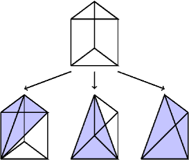
Figure 1: The splitting of a space–time prism into three tetrahedra.

Figure 2: A space–time tetrahedral mesh of a space–time slab $\mathcal{E}^{n}$.

Consider now a single space–time cell $\mathcal{K}_{j}\in\mathcal{T}^{n}$. The boundary of this space–time cell is denoted by $\partial\mathcal{K}_{j}$. The outward unit space–time normal vector on $\partial\mathcal{K}_{j}$ is given by $(n_{t}^{\mathcal{K}_{j}},\boldsymbol{n}^{\mathcal{K}_{j}})$. The boundary $\partial\mathcal{K}_{j}$ may consist of a facet on which $|n_{t}^{\mathcal{K}_{j}}|=1$ (which we denote by $K^{n}_{j}$ if $n_{t}^{\mathcal{K}_{j}}=-1$ or $K^{n+1}_{j}$ if $n_{t}^{\mathcal{K}_{j}}=1$) and $\mathcal{Q}_{\mathcal{K}_{j}}=\partial\mathcal{K}_{j}\backslash(K_{j}^{n}\cup K_{j}^{n+1})$. In the remainder of this paper, we will drop the sub- and superscript notatation when referring to the space–time normal vector and the space–time cell wherever no confusion will occur.

In a space–time slab $\mathcal{E}^{n}$, the set of all facets for which $\mathinner{\!\left\lvert n_{t}\right\rvert}\neq 1$ is denoted by $\mathcal{F}^{n}$ while the union of these facets is denoted by $\Gamma^{n}$. The set $\mathcal{F}^{n}$ is partitioned into a set of interior facets $\mathcal{F}_{I}^{n}$ and a set of facets that lie on the boundary of $\mathcal{E}^{n}$, $\mathcal{F}_{B}^{n}$, so that $\mathcal{F}^{n}=\mathcal{F}_{I}^{n}\cup\mathcal{F}_{B}^{n}$. We furthermore denote the set of facets that lie on the Neumann boundary, $\partial\mathcal{E}^{N}\cap\partial\mathcal{E}^{n}$, by $\mathcal{F}^{n}_{N}$.

We consider the following finite-dimensional function spaces on the space–time slab $\mathcal{E}^{n}$:

$$\boldsymbol{V}_{h}^{n} \mathrel{\mathop{\mathchar 58\relax}}=\mathinner{\left\{\boldsymbol{v}_{h}\in\mathinner{\left[L^{2}(\mathcal{T}^{n})\right]}^{d},\ \boldsymbol{v}_{h}\in\mathinner{\left[P_{k}(\mathcal{K})\right]}^{d}\ \forall\mathcal{K}\in\mathcal{T}^{n}\right\}},$$ (3a)

$$Q_{h}^{n} \mathrel{\mathop{\mathchar 58\relax}}=\mathinner{\left\{q_{h}\in L^{2}(\mathcal{T}^{n}),\ q_{h}\in P_{k-1}(\mathcal{K})\ \forall\mathcal{K}\in\mathcal{T}^{n}\right\}},$$ (3b)

where $P_{l}(D)$ denotes the space of polynomials of degree $l>0$ on a domain $D$. The left and right traces of a function $q_{h}\in Q_{h}^{n}$ at an interior facet $\mathcal{S}\in\mathcal{F}_{I}^{n}$ are denoted by $q_{h}^{l}$ and $q_{h}^{r}$. In general $q_{h}^{l}\neq q_{h}^{r}$ so that it will be useful to introduce the jump operator $[\![q_{h}\boldsymbol{n}]\!]=q_{h}^{l}\boldsymbol{n}^{l}+q_{h}^{r}\boldsymbol{n}^{r}$. On a boundary facet $\mathcal{S}\in\mathcal{F}_{B}^{n}$ the jump operator is defined as $[\![q_{h}\boldsymbol{n}]\!]=q_{h}\boldsymbol{n}$. Similar expressions hold for $\boldsymbol{v}_{h}\in\boldsymbol{V}_{h}^{n}$.

For the hybridized discontinuous Galerkin method, we require also finite dimensional function spaces on $\Gamma^{n}$:

$$\bar{\boldsymbol{V}}_{h}^{n} \mathrel{\mathop{\mathchar 58\relax}}=\mathinner{\left\{\bar{\boldsymbol{v}}_{h}\in\mathinner{\left[L^{2}(\mathcal{F}^{n})\right]}^{d},\ \bar{\boldsymbol{v}}_{h}\in\mathinner{\left[P_{k}(\mathcal{S})\right]}^{d}\ \forall\mathcal{S}\in\mathcal{F}^{n},\ \bar{\boldsymbol{v}}_{h}=0\ \text{on}\ \partial\mathcal{E}^{D}\cap\partial\mathcal{E}^{n}\right\}},$$ (4a)

$$\bar{Q}_{h}^{n} \mathrel{\mathop{\mathchar 58\relax}}=\mathinner{\left\{\bar{q}_{h}\in L^{2}(\mathcal{F}^{n}),\ \bar{q}_{h}\in P_{k}(\mathcal{S})\ \forall\mathcal{S}\in\mathcal{F}^{n}\right\}}.$$ (4b)

For notational purposes, we introduce the spaces $\boldsymbol{V}_{h}^{n,\star}=\boldsymbol{V}_{h}^{n}\times\bar{\boldsymbol{V}}_{h}^{n}$ and $Q_{h}^{n,\star}=Q_{h}^{n}\times\bar{Q}_{h}^{n}$. Functions pairs in $\boldsymbol{V}_{h}^{n,\star}$ and $Q_{h}^{n,\star}$ will be denoted by $\boldsymbol{v}_{h}^{\star}=(\boldsymbol{v}_{h},\bar{\boldsymbol{v}}_{h})\in\boldsymbol{V}_{h}^{n,\star}$ and $q_{h}^{\star}=(q_{h},\bar{q}_{h})\in Q_{h}^{n,\star}$.

3.2 The finite element variational formulation

We present now the finite element variational formulation of the Navier–Stokes problem on time-dependent domains. For this, consider first the steady Stokes problem on a time-dependent domain:

$$-\nu\nabla^{2}\boldsymbol{u}+\nabla p =\boldsymbol{f} \text{in}\ \mathcal{E},$$ (5a)

$$\nabla\cdot\boldsymbol{u} =0 \text{in}\ \mathcal{E},$$ (5b)

with boundary conditions

$$\boldsymbol{u} =\boldsymbol{0} \text{on}\ \partial\mathcal{E}^{D},$$ (6a)

$$\mathinner{\left(p\mathbb{I}-\nu\nabla\boldsymbol{u}\right)}\cdot\boldsymbol{n} =\boldsymbol{h} \text{on}\ \partial\mathcal{E}^{N},$$ (6b)

with $\boldsymbol{h}\mathrel{\mathop{\mathchar 58\relax}}\partial\mathcal{E}^{N}\to\mathbb{R}^{d}$ given Neumann boundary data. A straightforward extension of the hybridized discontinuous Galerkin method of [24] to the Stokes problem on time-dependent domains is given by: In each space–time slab $\mathcal{E}^{n}$, $n=0,1,\cdots,N-1$, we seek $(\boldsymbol{u}_{h}^{\star},p_{h}^{\star})\in\boldsymbol{V}_{h}^{n,\star}\times Q_{h}^{n,\star}$ such that

$$a_{h}^{n}(\boldsymbol{u}_{h}^{\star},\boldsymbol{v}_{h}^{\star})+b_{h}^{n}(p_{h}^{\star},\boldsymbol{v}_{h}^{\star})-b_{h}^{n}(q_{h}^{\star},\boldsymbol{u}_{h}^{\star})=\sum_{\mathcal{K}\in\mathcal{T}^{n}}\int_{\mathcal{K}}\boldsymbol{f}\cdot\boldsymbol{v}_{h}\operatorname{d\!}\boldsymbol{x}\operatorname{d\!}t-\sum_{\mathcal{S}\in\mathcal{F}^{n}_{N}}\int_{\mathcal{S}}\boldsymbol{h}\cdot\bar{\boldsymbol{v}}_{h}\operatorname{d\!}s,$$ (7)

for all $(\boldsymbol{v}_{h}^{\star},q_{h}^{\star})\in\boldsymbol{V}_{h}^{n,\star}\times Q_{h}^{n,\star}$, where

$$a_{h}^{n}(\boldsymbol{u}^{\star},\boldsymbol{v}^{\star})\mathrel{\mathop{\mathchar 58\relax}}= \sum_{\mathcal{K}\in\mathcal{T}^{n}}\int_{\mathcal{K}}\nu\nabla\boldsymbol{u}\mathrel{\mathop{\mathchar 58\relax}}\nabla\boldsymbol{v}\operatorname{d\!}\boldsymbol{x}\operatorname{d\!}t+\sum_{K\in\mathcal{T}^{n}}\int_{\mathcal{Q}_{\mathcal{K}}}\frac{\nu\alpha}{h_{\mathcal{K}}}(\boldsymbol{u}-\bar{\boldsymbol{u}})\cdot(\boldsymbol{v}-\bar{\boldsymbol{v}})\operatorname{d\!}s$$ (8a)

$$-\sum_{\mathcal{K}\in\mathcal{T}^{n}}\int_{\mathcal{Q}_{\mathcal{K}}}\nu\mathinner{\left[(\boldsymbol{u}-\bar{\boldsymbol{u}})\cdot\dfrac{\partial{}\boldsymbol{v}}{\partial{\boldsymbol{n}}}+\dfrac{\partial{}\boldsymbol{u}}{\partial{\boldsymbol{n}}}\cdot(\boldsymbol{v}-\bar{\boldsymbol{v}})\right]}\operatorname{d\!}s,$$

$$b_{h}^{n}(p^{\star},\boldsymbol{v}^{\star})\mathrel{\mathop{\mathchar 58\relax}}= -\sum_{\mathcal{K}\in\mathcal{T}^{n}}\int_{\mathcal{K}}p\nabla\cdot\boldsymbol{v}\operatorname{d\!}\boldsymbol{x}\operatorname{d\!}t+\sum_{\mathcal{K}\in\mathcal{T}^{n}}\int_{\mathcal{Q}_{\mathcal{K}}}(\boldsymbol{v}-\bar{\boldsymbol{v}})\cdot\boldsymbol{n}\bar{p}\operatorname{d\!}s.$$ (8b)

Here $\alpha>0$ is a penalty parameter that needs to be sufficiently large to ensure stability. These bi-linear forms are similar to those of [24, 14, 25] with the difference being that integration is over $d+1$-dimensional space–time cells $\mathcal{K}$, as opposed to $d$-dimensional spatial cells. Note furthermore that space–time slabs are completely independent of each other due to the Stokes equations eq. 5 not being time-dependent.

We will now discuss in more detail the variational formulation for the convective parts of the linearized Navier–Stokes equations. In particular, let $\boldsymbol{w}\mathrel{\mathop{\mathchar 58\relax}}\mathcal{E}\to\mathbb{R}^{d}$ be a given divergence-free and $H(\text{div})$-conforming velocity field. We will derive the discrete space–time variational formulation for

$$\partial_{t}\boldsymbol{u}+\nabla\cdot\mathinner{\left(\boldsymbol{u}\otimes\boldsymbol{w}\right)}=\boldsymbol{0}\qquad\text{in}\ \mathcal{E},$$ (9)

with boundary condition

$$(n_{t}+\boldsymbol{w}\cdot\boldsymbol{n})\boldsymbol{u}=\boldsymbol{r}\quad\text{on}\ \partial\mathcal{E}^{-},$$ (10)

where $\partial\mathcal{E}^{-}$ is the part of $\partial\mathcal{E}^{N}$ where $n_{t}+\boldsymbol{w}\cdot\boldsymbol{n}<0$, and where $\boldsymbol{r}\mathrel{\mathop{\mathchar 58\relax}}\partial\mathcal{E}^{-}\to\mathbb{R}^{d}$ is given boundary data. In each space–time slab $\mathcal{E}^{n}$, we multiply eq. 9 by a test function $\boldsymbol{v}_{h}\in\boldsymbol{V}_{h}^{n}$, integrate over a cell $\mathcal{K}\in\mathcal{T}^{n}$, approximate $\boldsymbol{w}$ by a divergence-free $\boldsymbol{w}_{h}\in\boldsymbol{V}_{h}^{n}\cap H({\rm div})$, apply Green’s identity in space–time and sum over all cells of the triangulation and over all space–time slabs,

$$\sum_{n=0}^{N-1}\bigg{(}-\sum_{\mathcal{K}\in\mathcal{T}^{n}}\int_{\mathcal{K}}\mathinner{\left(\boldsymbol{u}_{h}\cdot\partial_{t}\boldsymbol{v}_{h}+\boldsymbol{u}_{h}\otimes\boldsymbol{w}_{h}\mathrel{\mathop{\mathchar 58\relax}}\nabla\boldsymbol{v}_{h}\right)}\operatorname{d\!}\boldsymbol{x}\operatorname{d\!}t+\sum_{\mathcal{K}\in\mathcal{T}^{n}}\int_{\partial\mathcal{K}}H_{\mathcal{K}}^{n}(\boldsymbol{u}_{h}^{\star},\boldsymbol{w}_{h};n_{t},\boldsymbol{n})\cdot\boldsymbol{v}_{h}\operatorname{d\!}s\bigg{)}=0.$$ (11)

For stability purposes, the convective flux on the cell boundary $\partial\mathcal{K}$ in the space–time normal direction, $\mathinner{\left(n_{t}+\boldsymbol{w}_{h}\cdot\boldsymbol{n}\right)}\boldsymbol{u}_{h}$, was replaced by the space–time upwind flux

$$H_{\mathcal{K}}^{n}(\boldsymbol{u}_{h}^{\star},\boldsymbol{w}_{h};n_{t},\boldsymbol{n})=\begin{cases}\mathinner{\left(n_{t}+\boldsymbol{w}_{h}\cdot\boldsymbol{n}\right)}\mathinner{\left(\boldsymbol{u}_{h}+\lambda(\bar{\boldsymbol{u}}_{h}-\boldsymbol{u}_{h})\right)}&\text{on}\ \mathcal{Q}_{\mathcal{K}},\\ \boldsymbol{u}_{h}n_{t}&\text{on}\ K^{n+1},\\ \boldsymbol{u}_{h}^{-}n_{t}&\text{on}\ K^{n},\end{cases}$$ (12)

where, on $K^{n}$, $\boldsymbol{u}_{h}^{-}=\lim_{\varepsilon\to 0}\boldsymbol{u}_{h}(t_{n}-\varepsilon)$, and where $\lambda=1$ if $n_{t}+\boldsymbol{w}_{h}\cdot\boldsymbol{n}<0$ and $\lambda=0$ otherwise. Substituting this expression into eq. 11,

$$\sum_{n=0}^{N-1}\bigg{(}-\sum_{\mathcal{K}\in\mathcal{T}^{n}}\int_{\mathcal{K}}\mathinner{\left(\boldsymbol{u}_{h}\cdot\partial_{t}\boldsymbol{v}_{h}+\boldsymbol{u}_{h}\otimes\boldsymbol{w}_{h}\mathrel{\mathop{\mathchar 58\relax}}\nabla\boldsymbol{v}_{h}\right)}\operatorname{d\!}\boldsymbol{x}\operatorname{d\!}t+\sum_{\mathcal{K}\in\mathcal{T}^{n}}\int_{K^{n+1}}\boldsymbol{u}_{h}\cdot\boldsymbol{v}_{h}\operatorname{d\!}\boldsymbol{x}-\sum_{\mathcal{K}\in\mathcal{T}^{n}}\int_{K^{n}}\boldsymbol{u}_{h}^{-}\cdot\boldsymbol{v}_{h}\operatorname{d\!}\boldsymbol{x}\\ +\sum_{\mathcal{K}\in\mathcal{T}^{n}}\int_{\mathcal{Q}_{\mathcal{K}}}H_{\mathcal{K}}^{n}(\boldsymbol{u}_{h}^{\star},\boldsymbol{w}_{h};n_{t},\boldsymbol{n})\cdot\boldsymbol{v}_{h}\operatorname{d\!}s\bigg{)}=0,$$ (13)

where we used that $n_{t}=1$ on $K^{n+1}$ and $n_{t}=-1$ on $K^{n}$. Note that the numerical flux on the boundary of cell $\mathcal{K}$ depends only on the local cell unknown $\boldsymbol{u}_{h}$ and the facet unknown $\bar{\boldsymbol{u}}_{h}$. As such, the numerical flux on an interior facet $\mathcal{S}\in\mathcal{F}$, shared by two adjacent cells $\mathcal{K}^{+}$ and $\mathcal{K}^{-}$, need not be equal, i.e., $H_{\mathcal{K}^{+}}^{n}((\boldsymbol{u}_{h}^{+},\bar{\boldsymbol{u}}_{h}),\boldsymbol{w}_{h}^{+};n_{t}^{+},\boldsymbol{n}^{+})\neq H_{\mathcal{K}^{-}}^{n}((\boldsymbol{u}_{h}^{-},\bar{\boldsymbol{u}}_{h}),\boldsymbol{w}_{h}^{-};n_{t}^{-},\boldsymbol{n}^{-})$. In order to guarantee local conservation, we follow [21] and impose that the $L^{2}$-projection of the space–time normal component of the numerical flux into $\bar{\boldsymbol{V}}_{h}^{n}$ is single-valued:

$$\sum_{n=0}^{N-1}\mathinner{\left(\int_{\mathcal{K}\in\mathcal{T}^{n}}H_{\mathcal{K}}^{n}(\boldsymbol{u}_{h}^{\star},\boldsymbol{w}_{h};n_{t},\boldsymbol{n})\cdot\bar{\boldsymbol{v}}_{h}\operatorname{d\!}s-\int_{\partial\mathcal{E}^{+}}(n_{t}+\bar{\boldsymbol{w}}_{h}\cdot\boldsymbol{n})\bar{\boldsymbol{u}}_{h}\cdot\bar{\boldsymbol{v}}_{h}\operatorname{d\!}s\right)}=\sum_{n=0}^{N-1}\int_{\partial\mathcal{E}^{-}}\boldsymbol{r}\cdot\bar{\boldsymbol{v}}_{h}\operatorname{d\!}s,$$ (14)

where $\partial\mathcal{E}^{+}$ is the part of $\partial\mathcal{E}^{N}$ where $n_{t}+\boldsymbol{w}\cdot\boldsymbol{n}\geq 0$ and where we used the inflow boundary condition eq. 10. Subtracting eq. 14 from eq. 13, and noting that each space–time slab depends only on the previous space–time slab, so that we may drop the summation over space–time slabs, we find the following finite element variational formulation for eq. 9 and eq. 10: In each space–time slab $\mathcal{E}^{n}$, $n=0,\cdots,N-1$, we seek $\boldsymbol{u}_{h}^{\star}\in\boldsymbol{V}_{h}^{n,\star}$ such that

$$t_{h}^{n}(\boldsymbol{u}_{h}^{\star},\boldsymbol{w}_{h}^{\star},\boldsymbol{v}_{h}^{\star})=\sum_{\mathcal{K}\in\mathcal{T}^{n}}\int_{K^{n}}\boldsymbol{u}_{h}^{-}\cdot\boldsymbol{v}_{h}\operatorname{d\!}\boldsymbol{x}-\int_{\partial\mathcal{E}^{-}}\boldsymbol{r}\cdot\bar{\boldsymbol{v}}_{h}\operatorname{d\!}s,$$ (15)

where the tri-linear form for the convective term is defined as:

$$t_{h}^{n}(\boldsymbol{u}^{\star},\boldsymbol{w}^{\star},\boldsymbol{v}^{\star})=-\sum_{\mathcal{K}\in\mathcal{T}^{n}}\int_{\mathcal{K}}\mathinner{\left(\boldsymbol{u}\cdot\partial_{t}\boldsymbol{v}+\boldsymbol{u}\otimes\boldsymbol{w}\mathrel{\mathop{\mathchar 58\relax}}\nabla\boldsymbol{v}\right)}\operatorname{d\!}\boldsymbol{x}\operatorname{d\!}t+\sum_{\mathcal{K}\in\mathcal{T}^{n}}\int_{K^{n+1}}\boldsymbol{u}\cdot\boldsymbol{v}\operatorname{d\!}\boldsymbol{x}\\ +\sum_{\mathcal{K}\in\mathcal{T}^{n}}\int_{\mathcal{Q}_{\mathcal{K}}}H_{\mathcal{K}}^{n}(\boldsymbol{u}^{\star},\boldsymbol{w};n_{t},\boldsymbol{n})\cdot\mathinner{\left(\boldsymbol{v}-\bar{\boldsymbol{v}}\right)}\operatorname{d\!}s+\int_{\partial\mathcal{E}^{+}}(n_{t}+\bar{\boldsymbol{w}}\cdot\boldsymbol{n})\bar{\boldsymbol{u}}\cdot\bar{\boldsymbol{v}}\operatorname{d\!}s.$$ (16)

We remark that for $n=0$, $\boldsymbol{u}_{h}^{-}$ is the projection of the initial condition eq. 2c into $\boldsymbol{V}_{h}^{0}\cap H(\text{div})$ such that $\boldsymbol{u}_{h}^{-}$ is point-wise divergence free.

Combining eq. 7 and eq. 15, we conclude this section by stating the discontinuous Galerkin in time and space–time hybridized discontinuous Galerkin variational formulation for the incompressible Navier–Stokes problem eq. 1–eq. 2: In each space–time slab $\mathcal{E}^{n}$, $n=0,\cdots,N-1$, we seek $(\boldsymbol{u}_{h}^{\star},p_{h}^{\star})\in\boldsymbol{V}_{h}^{n,\star}\times Q_{h}^{n,\star}$ such that

$$t_{h}^{n}(\boldsymbol{u}_{h}^{\star},\boldsymbol{u}_{h}^{\star},\boldsymbol{v}_{h}^{\star})+a_{h}^{n}(\boldsymbol{u}_{h}^{\star},\boldsymbol{v}_{h}^{\star})+b_{h}^{n}(p_{h}^{\star},\boldsymbol{v}_{h}^{\star})-b_{h}^{n}(q_{h}^{\star},\boldsymbol{u}_{h}^{\star})=\sum_{\mathcal{K}\in\mathcal{T}^{n}}\int_{\mathcal{K}}\boldsymbol{f}\cdot\boldsymbol{v}_{h}\operatorname{d\!}\boldsymbol{x}\operatorname{d\!}t-\sum_{\mathcal{S}\in\mathcal{F}^{n}_{N}}\int_{\mathcal{S}}\boldsymbol{g}\cdot\bar{\boldsymbol{v}}_{h}\operatorname{d\!}s+\int_{\Omega_{n}}\boldsymbol{u}_{h}^{-}\cdot\boldsymbol{v}_{h}\operatorname{d\!}s,$$ (17)

for all $(\boldsymbol{v}_{h}^{\star},q_{h}^{\star})\in\boldsymbol{V}_{h}^{n,\star}\times Q_{h}^{n,\star}$.

Arbitrary Lagrangian Eulerian formulation

For practical implementations it may be preferable to consider the space–time hybridized discontinuous Galerkin variational formulation eq. 17 in arbitrary Lagrangian Eulerian (ALE) formulation. The ALE formulation is obtained by noting that the space–time normal on space–time cell boundaries $\mathcal{Q}_{\mathcal{K}}$ may be written as $(n_{t},\boldsymbol{n})=(-\boldsymbol{v}_{g}\cdot\boldsymbol{n},\boldsymbol{n})$, where $\boldsymbol{v}_{g}$ is the grid velocity [37]. Only the tri-linear form, $t_{h}^{n}(\boldsymbol{u}^{\star},\boldsymbol{w}^{\star},\boldsymbol{v}^{\star})$, needs to be rewritten in ALE formulation, since the other terms in the variational formulation do not depend on $n_{t}$. The ALE formulation of $t_{h}^{n}(\boldsymbol{u}^{\star},\boldsymbol{w}^{\star},\boldsymbol{v}^{\star})$ is given by

$$t_{h}^{n}(\boldsymbol{u}^{\star},\boldsymbol{w}^{\star},\boldsymbol{v}^{\star})=-\sum_{\mathcal{K}\in\mathcal{T}^{n}}\int_{\mathcal{K}}\mathinner{\left(\boldsymbol{u}\cdot\partial_{t}\boldsymbol{v}+\boldsymbol{u}\otimes\boldsymbol{w}\mathrel{\mathop{\mathchar 58\relax}}\nabla\boldsymbol{v}\right)}\operatorname{d\!}\boldsymbol{x}\operatorname{d\!}t+\sum_{\mathcal{K}\in\mathcal{T}^{n}}\int_{K^{n+1}}\boldsymbol{u}\cdot\boldsymbol{v}\operatorname{d\!}\boldsymbol{x}\\ +\sum_{\mathcal{K}\in\mathcal{T}^{n}}\int_{\mathcal{Q}_{\mathcal{K}}}G_{\mathcal{K}}^{n}(\boldsymbol{u}^{\star},\boldsymbol{w};\boldsymbol{v}_{g},\boldsymbol{n})\cdot\mathinner{\left(\boldsymbol{v}-\bar{\boldsymbol{v}}\right)}\operatorname{d\!}s+\int_{\partial\mathcal{E}^{+}}\mathinner{\left((\bar{\boldsymbol{w}}-\boldsymbol{v}_{g})\cdot\boldsymbol{n}\right)}\bar{\boldsymbol{u}}\cdot\bar{\boldsymbol{v}}\operatorname{d\!}s,$$ (18)

with numerical flux

$$G_{\mathcal{K}}^{n}(\boldsymbol{u}^{\star},\boldsymbol{w};\boldsymbol{v}_{g},\boldsymbol{n})=\mathinner{\left(\boldsymbol{u}_{h}+\lambda(\bar{\boldsymbol{u}}_{h}-\boldsymbol{u}_{h})\right)}(\boldsymbol{w}_{h}-\boldsymbol{v}_{g})\cdot\boldsymbol{n}.$$ (19)

4 Properties of the discrete variational formulation

To find the solution $(\boldsymbol{u}_{h}^{\star},p_{h}^{\star})\in\boldsymbol{V}_{h}^{n,\star}\times Q_{h}^{n,\star}$ to the non-linear variational formulation eq. 17, we use a Picard iteration scheme: in every space–time slab, given a solution $(\boldsymbol{u}_{h}^{\star,k},p_{h}^{\star,k})$ we seek a solution $(\boldsymbol{u}_{h}^{\star,k+1},p_{h}^{\star,k+1})$ in iteration $k+1$ that solves the linear variational formulation

$$t_{h}^{n}(\boldsymbol{u}_{h}^{\star,k+1},\boldsymbol{u}_{h}^{\star,k},\boldsymbol{v}_{h}^{\star})+a_{h}^{n}(\boldsymbol{u}_{h}^{\star,k+1},\boldsymbol{v}_{h}^{\star})+b_{h}^{n}(p_{h}^{\star,k+1},\boldsymbol{v}_{h}^{\star})-b_{h}^{n}(q_{h}^{\star},\boldsymbol{u}_{h}^{\star,k+1})=\\ \sum_{\mathcal{K}\in\mathcal{T}^{n}}\int_{\mathcal{K}}\boldsymbol{f}\cdot\boldsymbol{v}_{h}\operatorname{d\!}\boldsymbol{x}\operatorname{d\!}t-\sum_{\mathcal{S}\in\mathcal{F}^{n}_{N}}\int_{\mathcal{S}}\boldsymbol{g}\cdot\bar{\boldsymbol{v}}_{h}\operatorname{d\!}s+\int_{\Omega_{n}}\boldsymbol{u}_{h}^{-}\cdot\boldsymbol{v}_{h}\operatorname{d\!}s,$$ (20)

for all $(\boldsymbol{v}_{h}^{\star},q_{h}^{\star})\in\boldsymbol{V}_{h}^{n,\star}\times Q_{h}^{n,\star}$. The iterations are stopped when a certain convergence criterium has been met, at which point we set $(\boldsymbol{u}_{h}^{\star},p_{h}^{\star})=(\boldsymbol{u}_{h}^{\star,k+1},p_{h}^{\star,k+1})$.

The approximate velocity field $\boldsymbol{u}_{h}^{k}$ that is obtained at each Picard iteration $k$ is $H({\rm div})$-conforming and point-wise divergence-free in each space–time cell $\mathcal{K}\in\mathcal{T}^{n}$. To see this, we note that by taking $(\boldsymbol{v}_{h},\bar{\boldsymbol{v}}_{h},\bar{q}_{h})=(\boldsymbol{0},\boldsymbol{0},0)$ and $q_{h}=\nabla\cdot\boldsymbol{u}_{h}^{k}\in Q_{h}^{n}$ in eq. 17 results in

$$\int_{\mathcal{K}}(\nabla\cdot\boldsymbol{u}_{h}^{k})^{2}\operatorname{d\!}\boldsymbol{x}\operatorname{d\!}t=0\qquad\forall\mathcal{K}\in\mathcal{T}^{n},$$ (21)

from which it follows that $\nabla\cdot\boldsymbol{u}_{h}^{k}=0$ for $(\boldsymbol{x},t)\in\mathcal{K}$ and for each $\mathcal{K}\in\mathcal{T}^{n}$. Furthermore, taking $(\boldsymbol{v}_{h},\bar{\boldsymbol{v}}_{h},q_{h})=(\boldsymbol{0},\boldsymbol{0},0)$ and $\bar{q}_{h}=[\![(\boldsymbol{u}_{h}^{k}-\bar{\boldsymbol{u}}_{h}^{k})\cdot\boldsymbol{n}]\!]\in\bar{Q}_{h}^{n}$ in eq. 17 results in

$$\sum_{\mathcal{S}\in\mathcal{F}_{I}^{n}}\int_{\mathcal{S}}[\![\boldsymbol{u}_{h}^{k}\cdot\boldsymbol{n}]\!]^{2}\operatorname{d\!}\boldsymbol{x}\operatorname{d\!}t+\sum_{\mathcal{S}\in\mathcal{F}_{B}^{n}}\int_{\mathcal{S}}\mathinner{\left((\boldsymbol{u}_{h}^{k}-\bar{\boldsymbol{u}}_{h}^{k})\cdot\boldsymbol{n}\right)}^{2}\operatorname{d\!}\boldsymbol{x}\operatorname{d\!}t=0,$$ (22)

where we used that $\bar{\boldsymbol{u}}_{h}^{k}$ is single-valued on interior facets. It follows that $\boldsymbol{u}_{h}^{k}\cdot\boldsymbol{n}$ is single-valued on interior facets and $\boldsymbol{u}_{h}^{k}\cdot\boldsymbol{n}=\bar{\boldsymbol{u}}_{h}^{k}\cdot\boldsymbol{n}$ on boundary facets, i.e., $\boldsymbol{u}_{h}^{k}$ is $H({\rm div})$-conforming.

Many finite element methods result in discretizations of the Navier–Stokes equations that are either energy stable or locally conservative. The space–time HDG method eq. 17, however, is both simultaneously, even on time-dependent domains. To see this, note that by eq. 14 the $L^{2}$-projection of the space–time normal component of the numerical flux into $\bar{\boldsymbol{V}}_{h}^{n}$ is single-valued guaranteeing that the variational formulation eq. 17 is locally conservative. We next show that the space–time variational formulation eq. 17 is also energy stable.

Consider eq. 20 in the first space–time slab $\mathcal{E}_{n}$, $n=0$. Assume we are given a solution $(\boldsymbol{u}_{h}^{k},\bar{\boldsymbol{u}}_{h}^{k},p_{h}^{k},\bar{p}_{h}^{k})$ from Picard iteration $k$. For notational reasons, set $\boldsymbol{u}_{h}^{\star}=\boldsymbol{u}_{h}^{\star,k+1}$, $\boldsymbol{w}_{h}^{\star}=\boldsymbol{u}_{h}^{\star,k}$ and $p_{h}^{\star}=p_{h}^{\star,k+1}$. For homogeneous boundary conditions, $f=0$, and taking $(\boldsymbol{v}_{h}^{\star},q_{h}^{\star})=(\boldsymbol{u}_{h}^{\star},p_{h}^{\star})$ in eq. 20,

$$t_{h}^{0}(\boldsymbol{u}_{h}^{\star},\boldsymbol{w}_{h}^{\star},\boldsymbol{u}_{h}^{\star})+a_{h}^{0}(\boldsymbol{u}_{h}^{\star},\boldsymbol{u}_{h}^{\star})=\int_{\Omega_{0}}\boldsymbol{u}_{h}^{-}\cdot\boldsymbol{u}_{h}\operatorname{d\!}s,$$ (23)

with the projection of the initial condition eq. 2c into $\boldsymbol{V}_{h}^{0}\cap H(\text{div})$ is such that $\boldsymbol{u}_{h}^{-}$ is point-wise divergence-free. Consider first the tri-linear form, $t_{h}^{0}(\boldsymbol{u}_{h}^{\star},\boldsymbol{w}_{h}^{\star},\boldsymbol{u}_{h}^{\star})$, and note that

$$t_{h}^{0}(\boldsymbol{u}_{h}^{\star},\boldsymbol{w}_{h}^{\star},\boldsymbol{u}_{h}^{\star})\mathrel{\mathop{\mathchar 58\relax}}=\sum_{\mathcal{K}\in\mathcal{T}^{0}}\int_{K^{1}}\mathinner{\!\left\lvert\boldsymbol{u}_{h}\right\rvert}^{2}\operatorname{d\!}\boldsymbol{x}-\sum_{\mathcal{K}\in\mathcal{T}^{0}}\int_{\mathcal{K}}\tfrac{1}{2}\mathinner{\left(\partial_{t}\mathinner{\!\left\lvert\boldsymbol{u}_{h}\right\rvert}^{2}+\nabla\cdot\mathinner{\left((\boldsymbol{u}_{h}\otimes\boldsymbol{w}_{h})\cdot\boldsymbol{u}_{h}\right)}\right)}\operatorname{d\!}\boldsymbol{x}\operatorname{d\!}t\\ +\sum_{\mathcal{K}\in\mathcal{T}^{0}}\int_{\mathcal{Q}^{0}_{\mathcal{K}}}\tfrac{1}{2}(n_{t}+\boldsymbol{w}_{h}\cdot\boldsymbol{n})\mathinner{\!\left\lvert\boldsymbol{u}_{h}\right\rvert}^{2}\operatorname{d\!}s-\sum_{\mathcal{K}\in\mathcal{T}^{0}}\int_{\mathcal{Q}^{0}_{\mathcal{K}}}\tfrac{1}{2}(n_{t}+\boldsymbol{w}_{h}\cdot\boldsymbol{n})\mathinner{\!\left\lvert\bar{\boldsymbol{u}}_{h}\right\rvert}^{2}\operatorname{d\!}s\\ +\int_{\partial\mathcal{E}^{N}\cap I_{0}}\max(n_{t}+\bar{\boldsymbol{w}}_{h}\cdot\boldsymbol{n},0)\mathinner{\!\left\lvert\bar{\boldsymbol{u}}_{h}\right\rvert}^{2}\operatorname{d\!}s+\sum_{\mathcal{K}\in\mathcal{T}^{0}}\int_{\mathcal{Q}^{0}_{\mathcal{K}}}\tfrac{1}{2}\mathinner{\!\left\lvert n_{t}+\boldsymbol{w}_{h}\cdot\boldsymbol{n}\right\rvert}\mathinner{\!\left\lvert\boldsymbol{u}_{h}-\bar{\boldsymbol{u}}_{h}\right\rvert}^{2}\operatorname{d\!}s.$$ (24)

Using that

$$\sum_{\mathcal{K}\in\mathcal{T}^{0}}\int_{\mathcal{K}}\partial_{t}\mathinner{\!\left\lvert\boldsymbol{u}_{h}\right\rvert}^{2}\operatorname{d\!}\boldsymbol{x}\operatorname{d\!}t=\sum_{\mathcal{K}\in\mathcal{T}^{0}}\int_{K^{1}}\mathinner{\!\left\lvert\boldsymbol{u}_{h}\right\rvert}^{2}\operatorname{d\!}\boldsymbol{x}-\sum_{\mathcal{K}\in\mathcal{T}^{0}}\int_{K^{0}}\mathinner{\!\left\lvert\boldsymbol{u}_{h}\right\rvert}^{2}\operatorname{d\!}\boldsymbol{x}+\sum_{\mathcal{K}\in\mathcal{T}^{0}}\int_{\mathcal{Q}^{0}_{\mathcal{K}}}\mathinner{\!\left\lvert\boldsymbol{u}_{h}\right\rvert}^{2}n_{t}\operatorname{d\!}s,$$ (25)

and

$$\sum_{\mathcal{K}\in\mathcal{T}^{0}}\int_{\mathcal{K}}\nabla\cdot\mathinner{\left((\boldsymbol{u}_{h}\otimes\boldsymbol{w}_{h})\cdot\boldsymbol{u}_{h}\right)}\operatorname{d\!}x =\sum_{\mathcal{K}\in\mathcal{T}^{0}}\int_{\mathcal{Q}^{0}_{\mathcal{K}}}\boldsymbol{w}_{h}\cdot\boldsymbol{n}\mathinner{\!\left\lvert\boldsymbol{u}_{h}\right\rvert}^{2}\operatorname{d\!}s,$$ (26)

$$\sum_{\mathcal{K}\in\mathcal{T}^{0}}\int_{\mathcal{Q}^{0}_{\mathcal{K}}}(n_{t}+\boldsymbol{w}_{h}\cdot\boldsymbol{n})\mathinner{\!\left\lvert\bar{\boldsymbol{u}}_{h}\right\rvert}^{2}\operatorname{d\!}s =\int_{\partial\mathcal{E}^{N}\cap I_{0}}(n_{t}+\bar{\boldsymbol{w}}_{h}\cdot\boldsymbol{n})\mathinner{\!\left\lvert\bar{\boldsymbol{u}}_{h}\right\rvert}^{2}\operatorname{d\!}s,$$ (27)

where the second equality is by single-valuedness of $\bar{\boldsymbol{u}}_{h}$ on facets and since $\boldsymbol{w}_{h}$ is $H({\rm div})$-conforming. Combining eq. 24–eq. 27, and simplifying terms,

$$t_{h}^{0}(\boldsymbol{u}_{h}^{\star},\boldsymbol{w}_{h}^{\star},\boldsymbol{u}_{h}^{\star})=\sum_{\mathcal{K}\in\mathcal{T}^{0}}\int_{K^{1}}\tfrac{1}{2}\mathinner{\!\left\lvert\boldsymbol{u}_{h}\right\rvert}^{2}\operatorname{d\!}\boldsymbol{x}+\sum_{\mathcal{K}\in\mathcal{T}^{0}}\int_{K^{0}}\tfrac{1}{2}\mathinner{\!\left\lvert\boldsymbol{u}_{h}\right\rvert}^{2}\operatorname{d\!}\boldsymbol{x}\\ +\sum_{\mathcal{K}\in\mathcal{T}^{0}}\int_{\mathcal{Q}^{0}_{\mathcal{K}}}\tfrac{1}{2}\mathinner{\!\left\lvert n_{t}+\boldsymbol{w}_{h}\cdot\boldsymbol{n}\right\rvert}\mathinner{\!\left\lvert\boldsymbol{u}_{h}-\bar{\boldsymbol{u}}_{h}\right\rvert}^{2}\operatorname{d\!}s+\int_{\partial\mathcal{E}^{N}\cap I_{0}}\frac{1}{2}\mathinner{\!\left\lvert n_{t}+\bar{\boldsymbol{w}}_{h}\cdot\boldsymbol{n}\right\rvert}\mathinner{\!\left\lvert\bar{\boldsymbol{u}}_{h}\right\rvert}^{2}\operatorname{d\!}s.$$ (28)

Combining eq. 28 with eq. 23, and using that $a_{h}^{0}(\boldsymbol{u}_{h}^{\star},\boldsymbol{u}_{h}^{\star})\geq 0$ for $\alpha$ large enough (see [14, 25, 24]), we obtain

$$\int_{\Omega_{1}}\tfrac{1}{2}\mathinner{\!\left\lvert\boldsymbol{u}_{h}\right\rvert}^{2}\operatorname{d\!}\boldsymbol{x}+\int_{\Omega_{0}}\tfrac{1}{2}\mathinner{\!\left\lvert\boldsymbol{u}_{h}\right\rvert}^{2}\operatorname{d\!}\boldsymbol{x}-\int_{\Omega_{0}}\boldsymbol{u}_{h}^{-}\cdot\boldsymbol{u}_{h}\operatorname{d\!}\boldsymbol{x}\leq 0.$$ (29)

Using that $2\boldsymbol{u}_{h}^{-}\cdot\boldsymbol{u}_{h}=|\boldsymbol{u}_{h}|^{2}+|\boldsymbol{u}_{h}^{-}|^{2}-|\boldsymbol{u}_{h}-\boldsymbol{u}_{h}^{-}|^{2}$, energy stability follows for each Picard iteration:

$$\int_{\Omega_{1}}\mathinner{\!\left\lvert\boldsymbol{u}_{h}\right\rvert}^{2}\operatorname{d\!}\boldsymbol{x}\leq\int_{\Omega_{0}}\mathinner{\!\left\lvert\boldsymbol{u}_{h}^{-}\right\rvert}^{2}\operatorname{d\!}\boldsymbol{x}.$$ (30)

Energy stability is now proven by induction for all $n>0$ by using $\boldsymbol{u}_{h}$ from space–time slab $\mathcal{E}_{n-1}$ as initial condition for the variational formulation eq. 20 in space–time slab $\mathcal{E}_{n}$. We have therefore shown that our space–time variational formulation is both energy stable and locally conservative, even on dynamic meshes.

5 Numerical examples

All simulations were implemented using the Modular Finite Element Method (MFEM) library [11]. Furthermore, for all simulations we use the penalty parameter $\alpha=6k^{2}$.

In each space–time slab $\mathcal{E}^{n}$ ($n=0,\cdots,N-1$) we solve the Navier–Stokes equations by Picard iteration eq. 20 with stopping criterion

$$\max\left\{\frac{\|\boldsymbol{u}^{k}_{h}-\boldsymbol{u}^{k-1}_{h}\|_{\infty}}{\|\boldsymbol{u}^{k}_{h}-\boldsymbol{u}^{0}_{h}\|_{\infty}},\frac{\|p^{k}_{h}-p^{k-1}_{h}\|_{\infty}}{\|p^{k}_{h}-p^{0}_{h}\|_{\infty}}\right\}<\text{TOL},$$ (31)

where $\|\cdot\|_{\infty}$ is the discrete $l^{\infty}$-norm and TOL is a user given parameter.

Let $U\in\mathbb{R}^{\dim\boldsymbol{V}^{n}_{h}},P\in\mathbb{R}^{\dim Q^{n}_{h}},\bar{U}\in\mathbb{R}^{\dim\bar{\boldsymbol{V}}^{n}_{h}},\bar{P}\in\mathbb{R}^{\dim\bar{Q}^{n}_{h}}$ be the vectors of coefficients of ${\boldsymbol{u}}_{h},p_{h},\bar{\boldsymbol{u}}_{h},\bar{p}_{h}$ with respect to the basis of the corresponding vector spaces. Then $W^{T}=[U^{T}\ P^{T}]$ is the vector of all element degrees-of-freedom and $\bar{W}^{T}=[\bar{U}^{T}\ \bar{P}^{T}]$ is the vector of all facet degrees-of-freedom. At each Picard iteration eq. 20 a linear system of the following block-matrix structure needs to be solved:

$$\begin{bmatrix}A&B\\ C&D\end{bmatrix}\begin{bmatrix}W\\ \bar{W}\end{bmatrix}=\begin{bmatrix}F\\ \bar{F}\end{bmatrix}.$$ (32)

As with all other hybridizable discontinuous Galerkin methods, $A$ has a block-diagonal structure. It is therefore cheap to eliminate $W$ from eq. 32 to obtain the reduced linear system $(-CA^{-1}B+D)\bar{W}=\bar{F}-CA^{-1}F$. We use the direct solver of MUMPS [2, 3] through PETSc [6, 5, 4] to solve this system of linear equations. Given $\bar{W}$ we can then compute $W$ cell-wise according to $W=A^{-1}(F-B\bar{W})$.

5.1 Convergence rates and pressure-robustness

In this first test case we compute the rates of convergence of the space–time HDG method applied to the Navier–Stokes equations on a time-dependent domain. Introducing first a uniform triangular mesh for the unit square, the mesh vertices $(x_{1},x_{2})$ for the deforming domain $\Omega(t)$ are obtained at any time $t\in[0,1]$ by the following relation

$$x_{i}=x_{i}^{0}+0.05(1-x_{i}^{0})\sin(2\pi(\tfrac{1}{2}-x_{i}^{*}+t))\qquad i=1,2,$$

where $(x_{1}^{0},x_{2}^{0})\in[0,1]^{2}$ are the vertices of the uniform mesh and $(x_{1}^{*},x_{2}^{*})=(x_{2}^{0},x_{1}^{0})$. The mesh at three different points in time is shown in fig. 3.

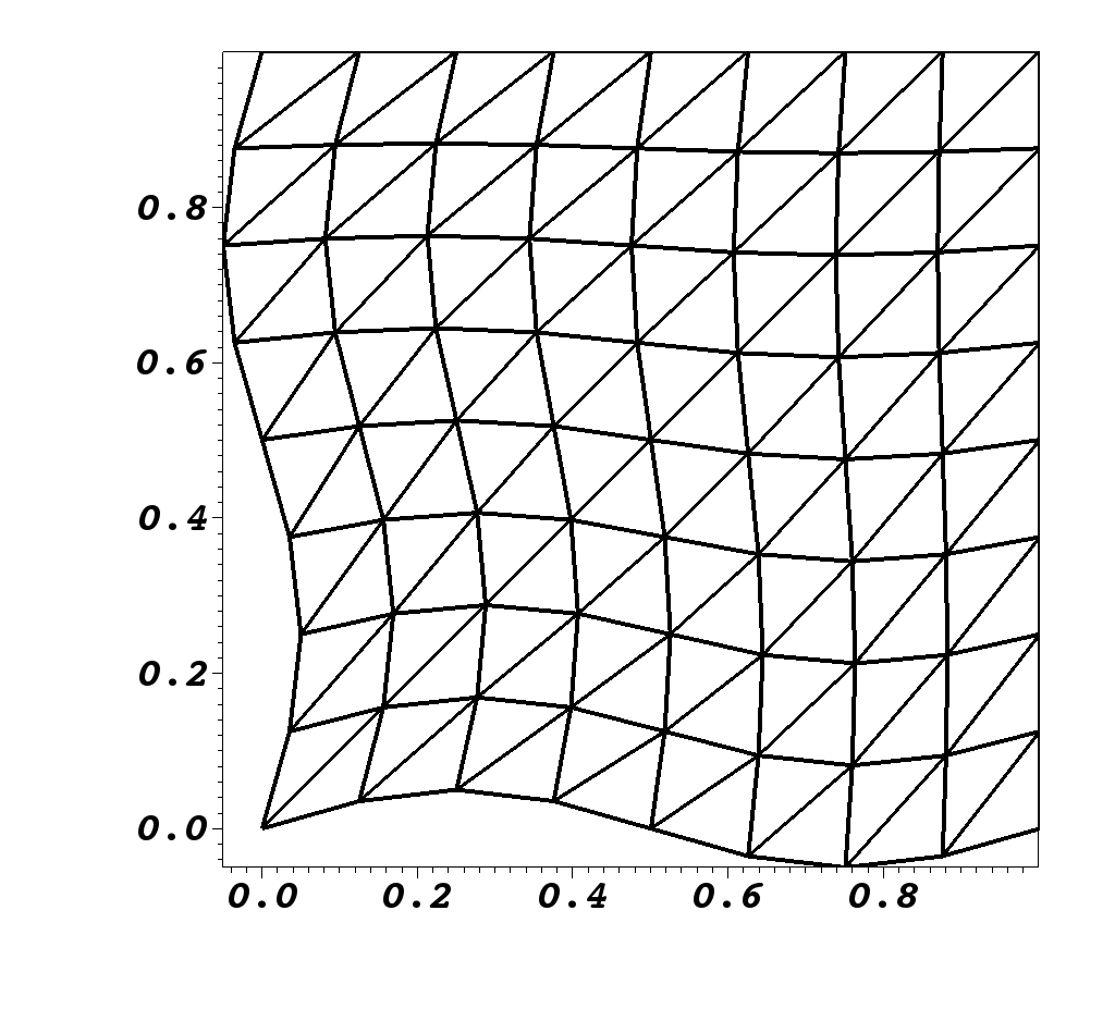
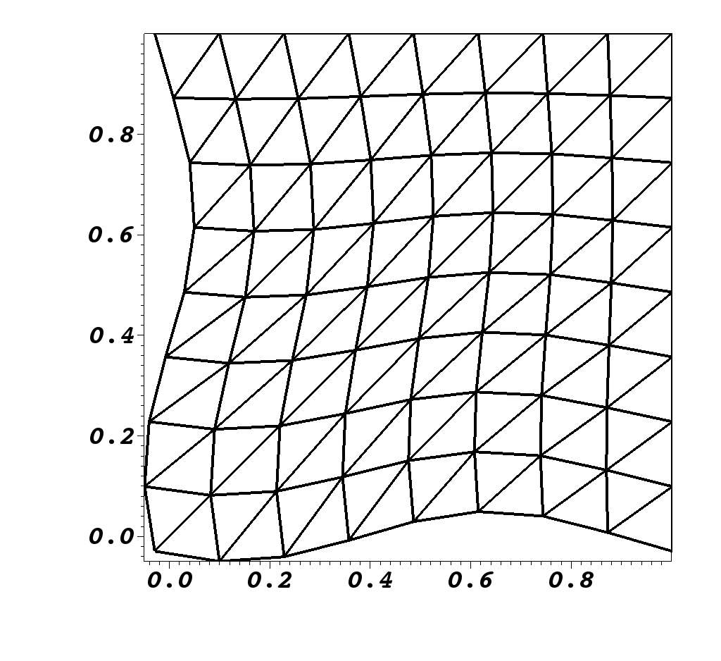
Figure 3: The mesh at different points in time for the test case of section 5.1. From left to right the mesh at $t=0,0.4,0.8$.

Let $\partial\mathcal{E}^{N}\mathrel{\mathop{\mathchar 58\relax}}=\mathinner{\left\{(t,x_{1},x_{2})\in\partial\mathcal{E}\mathrel{\mathop{\mathchar 58\relax}}x_{1}=1\right\}}$ and $\partial\mathcal{E}^{D}=\partial\mathcal{E}\setminus(\partial\mathcal{E}^{N}\cup\Omega(0)\cup(\Omega(1))$. The boundary conditions and source term $\boldsymbol{f}$ in eq. 1 are chosen such that the exact solution is given by

$$\boldsymbol{u}=\begin{bmatrix}(e^{t}-1)\sin(\pi x_{1})\sin(\pi x_{2})\\ (e^{t}-1)\cos(\pi x_{1})\cos(\pi x_{2})\end{bmatrix},\qquad p=(2+\cos(t))\sin(\pi x_{1})\cos(\pi x_{2}).$$

We consider the rates of convergence for polynomial degrees $k=2$ and $k=3$ and on a succession of refined space–time meshes. The coarsest space–time mesh consists of $6\cdot 8^{2}$ tetrahedra per space–time slab with $\Delta t=0.05$ and refinement happens in both space and time. For the Picard iteration eq. 31 we set $\text{TOL}=10^{-12}$.

Tables 1 and 2 show the rates of convergence for the velocity and pressure computed on the spatial domain at final time $T=1$ for $\nu=10^{-4}$ and $\nu=10^{-7}$, respectively. The rates of convergence over the entire space–time domain $\mathcal{E}$ are shown in tables 3 and 4 again for both $\nu=10^{-4}$ and $\nu=10^{-7}$. We observe from these tables, that for $k=2$ and for $k=3$, the method is optimal, i.e., the velocity error is of order $\mathcal{O}(h^{k+1})$ and the pressure error is of order $\mathcal{O}(h^{k})$. The tables also show that the error in the divergence of the approximate velocity is of machine precision even on deforming domains, as expected from section 4.

Finally, we observe that the velocity error is independent of the viscosity, i.e., the space–time hybridizable discontinuous Galerkin method eq. 17 is pressure-robust, even on time-dependent domains.

Cells per slab	Nr. of slabs	$\mathinner{\!\left\lVert\boldsymbol{u}-\boldsymbol{u}_{h}\right\rVert}$	rates	$\mathinner{\!\left\lVert p-p_{h}\right\rVert}$	rates	$\mathinner{\!\left\lVert\nabla\cdot\boldsymbol{u}_{h}\right\rVert}$
$\nu=10^{-4}$
$384$	$20$	1.5e-3	-	1.8e-2	-	6.0e-14
$1536$	$40$	2.0e-4	2.9	4.5e-3	2.0	1.1e-13
$6144$	$80$	2.6e-5	2.9	1.1e-3	2.0	2.4e-13
$24576$	$160$	3.3e-6	3.0	2.9e-4	1.9	4.7e-13
$\nu=10^{-7}$
$384$	$20$	1.5e-3	-	1.8e-2	-	6.0e-14
$1536$	$40$	2.0e-4	2.9	4.5e-3	2.0	1.2e-13
$6144$	$80$	2.5e-5	3.0	1.2e-3	1.9	2.5e-13
$24576$	$160$	3.3e-6	2.9	2.9e-4	2.0	5.0e-13

Table 1: The rates of convergence for the test case of section 5.1 with $k=2$ computed in the $L^{2}$-norm on $\Omega(T)$, the spatial domain at final time $T=1$.

Cells per slab	Nr. of slabs	$\mathinner{\!\left\lVert\boldsymbol{u}-\boldsymbol{u}_{h}\right\rVert}$	rates	$\mathinner{\!\left\lVert p-p_{h}\right\rVert}$	rates	$\mathinner{\!\left\lVert\nabla\cdot\boldsymbol{u}_{h}\right\rVert}$
$\nu=10^{-4}$
$384$	$20$	8.5e-5	-	1.3e-3	-	8.9e-13
$1536$	$40$	5.2e-6	4.0	1.6e-4	3.0	1.8e-12
$6144$	$80$	3.2e-7	4.0	2.0e-5	3.0	3.7e-12
$24576$	$160$	2.0e-8	4.0	2.5e-6	3.0	7.6e-12
$\nu=10^{-7}$
$384$	$20$	8.8e-5	-	1.3e-3	-	8.9e-13
$1536$	$40$	5.6e-6	4.0	1.6e-4	3.0	1.9e-12
$6144$	$80$	3.8e-7	3.9	2.0e-5	3.0	3.8e-12
$24576$	$160$	2.8e-8	3.8	2.5e-6	3.0	7.6e-12

Table 2: The rates of convergence for the test case of section 5.1 with $k=3$ computed in the $L^{2}$-norm on $\Omega(T)$, the spatial domain at final time $T=1$.

Cells per slab	Nr. of slabs	$\mathinner{\!\left\lVert\boldsymbol{u}-\boldsymbol{u}_{h}\right\rVert}$	rates	$\mathinner{\!\left\lVert p-p_{h}\right\rVert}$	rates	$\mathinner{\!\left\lVert\nabla\cdot\boldsymbol{u}_{h}\right\rVert}$
$\nu=10^{-4}$
$384$	$20$	6.9e-4	-	6.8e-3	-	4.2e-14
$1536$	$40$	8.8e-5	3.0	1.7e-3	2.0	8.3e-14
$6144$	$80$	1.2e-5	2.9	4.3e-4	2.0	1.6e-13
$24576$	$160$	1.5e-6	3.0	1.1e-4	2.0	3.0e-13
$\nu=10^{-7}$
$384$	$20$	6.9e-4	-	6.8e-3	-	4.3e-14
$1536$	$40$	8.6e-5	2.9	1.7e-3	2.0	8.9e-14
$6144$	$80$	1.1e-5	2.9	4.3e-4	2.0	1.8e-13
$24576$	$160$	1.4e-6	2.9	1.1e-4	2.0	3.5e-13

Table 3: The rates of convergence for the test case of section 5.1 with $k=2$ computed in the $L^{2}$-norm on $\mathcal{E}$, the whole space–time domain.

Cells per slab	Nr. of slabs	$\mathinner{\!\left\lVert\boldsymbol{u}-\boldsymbol{u}_{h}\right\rVert}$	rates	$\mathinner{\!\left\lVert p-p_{h}\right\rVert}$	rates	$\mathinner{\!\left\lVert\nabla\cdot\boldsymbol{u}_{h}\right\rVert}$
$\nu=10^{-4}$
$384$	$20$	3.4e-5	-	3.4e-4	-	6.8e-13
$1536$	$40$	2.1e-6	4.0	4.3e-5	3.0	1.4e-12
$6144$	$80$	1.2e-7	4.1	5.4e-6	3.0	2.7e-12
$24576$	$160$	7.5e-9	4.0	6.8e-7	3.0	5.5e-12
$\nu=10^{-7}$
$384$	$20$	3.5e-5	-	3.4e-4	-	6.8e-13
$1536$	$40$	2.3e-6	3.9	4.3e-5	3.0	1.4e-12
$6144$	$80$	1.5e-7	3.9	5.4e-6	3.0	2.8e-12
$24576$	$160$	1.1e-8	3.8	6.8e-7	3.0	5.6e-12

Table 4: The rates of convergence for the test case of section 5.1 with $k=3$ computed in the $L^{2}$-norm on $\mathcal{E}$, the whole space–time domain.

5.2 Flow around a cylinder

Next we consider flow around a cylinder. The setup of this test case is taken from [29, 15] in which we consider a fixed spatial domain $[0;2.2]\times[0;0.41]$ with a cylindrical obstacle with radius $r=0.05$ centred at $(x_{1},x_{2})=(0.2,0.2)$.

A homogeneous Neumann boundary condition is applied on the outflow boundary at $x_{1}=2.2$. On the inflow boundary at $x_{1}=0$ we impose $\boldsymbol{u}=[6x_{2}(0.41-x_{2})/0.41^{2},0]^{T}$, while $\boldsymbol{u}=\boldsymbol{0}$ is imposed on the cylinder and on the walls $x_{2}=0$ and $x_{2}=0.41$. The kinematic viscosity is set to be $\nu=10^{-3}$ and the initial condition is obtained by solving the steady–state Stokes problem, as done also in [25]. For the stopping criterion of the Picard iteration we used $\text{TOL}=10^{-9}$. The velocity magnitude at final time $t=5$ is shown in fig. 4.

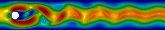
Figure 4: The velocity magnitude of flow around a cylinder, as described in section 5.2, at $t=5$ using $3222$ triangles and $k=3$.

To validate the dicretization we compute the lift and drag coefficients. These are defined as

$$C_{L}=\frac{1}{r\Delta t}\int_{\Gamma_{c}}(\sigma_{d}\cdot\boldsymbol{n})\cdot\boldsymbol{e}_{1},\qquad C_{D}=\frac{1}{r\Delta t}\int_{\Gamma_{c}}(\sigma_{d}\cdot\boldsymbol{n})\cdot\boldsymbol{e}_{2},$$

where $\boldsymbol{e}_{1}$ and $\boldsymbol{e}_{2}$ are the unit vectors in the $x_{1}$ and $x_{2}$ directions, respectively, and $\Gamma_{c}$ denotes the space–time boundary of the cylinder.

We compute the lift and drag coefficients on a space–time mesh consisting of $9666$ tetrahedra per slab. We consider a time step of $\Delta t=5\cdot 10^{-3}$. Over the time interval $t\in[0,5]$ we found that $C_{L}\in[-1.014,0.98]$ and $C_{D}\in[3.153,3.219]$, which compare well to the results found in literature [29, 15].

5.3 Flow around an oscillating airfoil

In this final test case we consider the simulation of flow around an oscillating NACA0012 airfoil on the domain $[-5,10]\times[-5,5]$ with trailing edge at the origin. The computational domain consists of 17088 tetrahedra per space–time slab and as polynomial approximation we use $k=2$. We set the kinematic viscosity to be $\nu=10^{-3}$. As stopping criterion in the Picard iteration we use $\text{TOL}=10^{-6}$.

To obtain the initial condition we first solve the steady Stokes problem around the airfoil at an angle of attack of $20^{\circ}$. We then solve the Navier–Stokes problem around the fixed airfoil from $t=0$ to $t=1$ using a time step of $\Delta t=0.01$. Given this ‘initial condition’ we then prescribe an oscillatory movement of the airfoil for $t>1$. Keeping the trailing edge fixed at $(x_{1},x_{2})=(0,0)$, the angle of attack changes according to

$$\text{angle of attack}=20+10\sin(\pi(t-1)).$$

For $t>1$ we use $\Delta t=2\cdot 10^{-3}$. To account for the time dependent angle of attack, the mesh is updated at each time step as follows. Nodes within a radius of $1.5$ from the trailing edge move with the airfoil, nodes outside a radius of $2$ from the trailing edge remain fixed, while the movement of the remaining nodes decrease linearly with distance, see fig. 5.

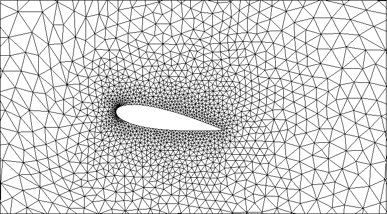
(a) Mesh at $10^{\circ}$ angle of attack.

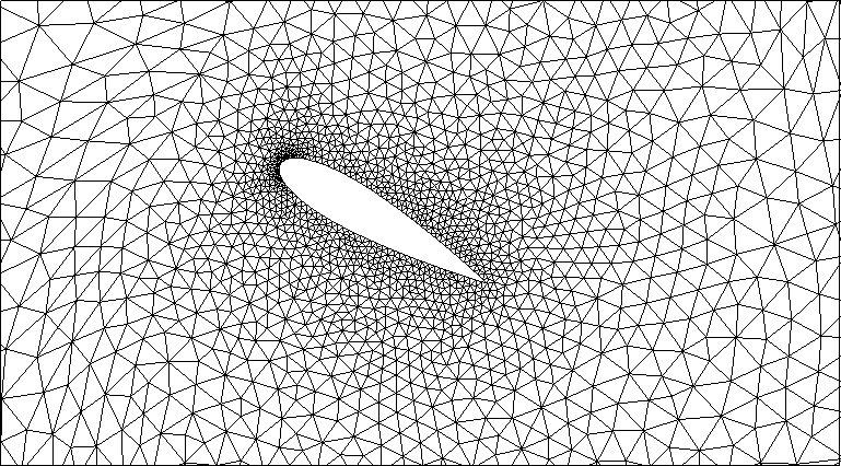
(b) Mesh at $30^{\circ}$ angle of attack.

Figure 5: Mesh at different angles of attack for the test case described in section 5.3.

In fig. 6 we plot the computed pressure and velocity vector fields. We observe vortex shedding at the trailing edge and detachment of vortices over the top of the airfoil while new vortices form at the tip of the airfoil. These phenomena agree with those observed in literature, for example [33].

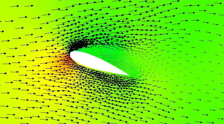
(a) Airfoil at $20^{\circ}$ angle of attack at $t=1$.

(b) Airfoil at $30^{\circ}$ angle of attack at $t=1.5$.

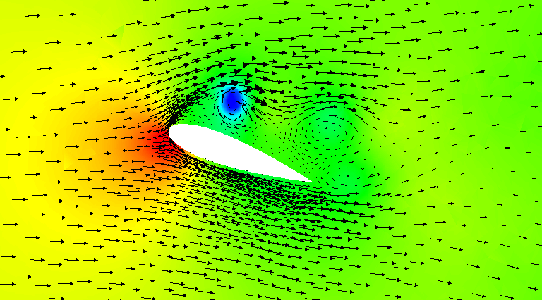
(c) Airfoil at $20^{\circ}$ angle of attack at $t=2$.

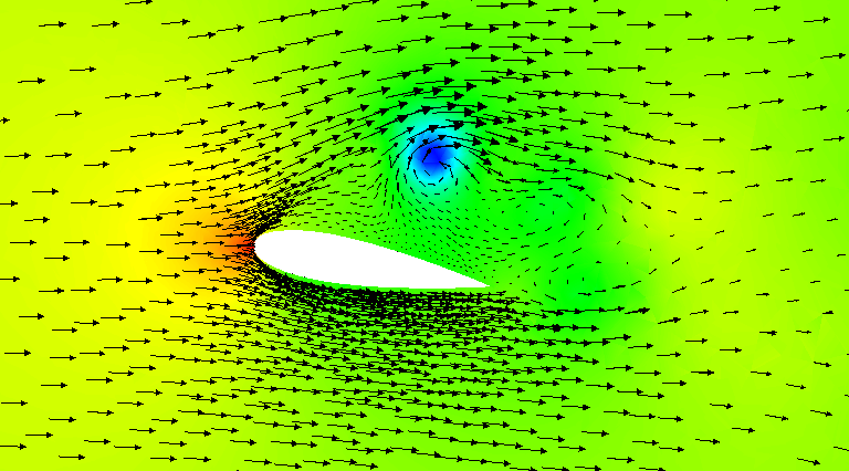
(d) Airfoil at $10^{\circ}$ angle of attack at $t=2.5$.

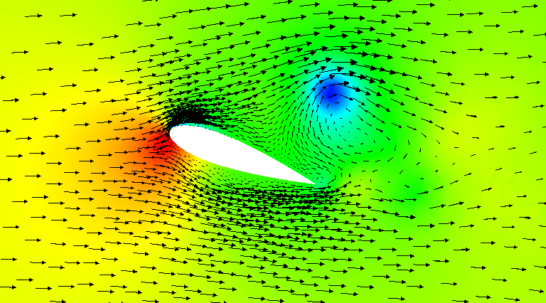
(e) Airfoil at $20^{\circ}$ angle of attack at $t=3$.

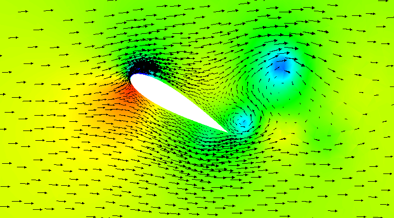
(f) Airfoil at $30^{\circ}$ angle of attack at $t=3.5$.

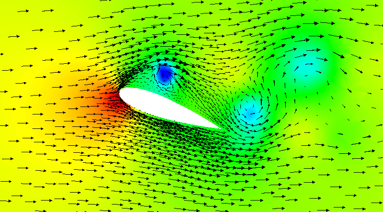
(g) Airfoil at $20^{\circ}$ angle of attack at $t=4$.

Figure 6: Velocity vector plot and pressure field around an oscillating NACA0012 airfoil as described in section 5.3.

6 Conclusions

We presented a space–time hybridizable discontinuous Galerkin finite element method for the Navier–Stokes equations on time-dependent domains. This scheme guarantees a point-wise divergence-free and $H({\rm div})$-conforming velocity field, it is locally momentum conserving and energy stable, even on dynamic meshes. We have shown the performance of the method in terms of rates of convergence, pressure-robustness, and flow simulations around a cylinder and an oscillating airfoil.

References

- Ambati and Bokhove [2007] V. Ambati and O. Bokhove. Space–time discontinuous Galerkin discretization of rotating shallow water equations. J. Comput. Phys., 225(2):1233–1261, 2007. doi: 10.1016/j.jcp.2007.01.036.
- Amestoy et al. [2001] P. Amestoy, I. Duff, J.-Y. L’Excellent, and J. Koster. A fully asynchronous multifrontal solver using distributed dynamic scheduling. SIAM J. Matrix Anal. & Appl., 23(1):15–41, 2001. doi: 10.1137/S0895479899358194.
- Amestoy et al. [2006] P. R. Amestoy, A. Guermouche, J.-Y. L’Excellent, and S. Pralet. Hybrid scheduling for the parallel solution of linear systems. Parallel Comput., 32(2):136–156, 2006. doi: 10.1016/j.parco.2005.07.004.
- Balay et al. [1997] S. Balay, W. D. Gropp, L. C. McInnes, and B. F. Smith. Efficient management of parallelism in object oriented numerical software libraries. In E. Arge, A. M. Bruaset, and H. P. Langtangen, editors, Modern Software Tools in Scientific Computing, pages 163–202. , Birkhäuser Press, 1997.
- Balay et al. [2016b] S. Balay, S. Abhyankar, M. F. Adams, J. Brown, P. Brune, K. Buschelman, L. Dalcin, V. Eijkhout, W. D. Gropp, D. Kaushik, M. G. Knepley, L. C. McInnes, K. Rupp, B. F. Smith, S. Zampini, H. Zhang, and H. Zhang. PETSc users manual. Technical Report ANL-95/11 - Revision 3.7, Argonne National Laboratory, 2016b. URL http://www.mcs.anl.gov/petsc.
- Balay et al. [2016a] S. Balay, S. Abhyankar, M. F. Adams, J. Brown, P. Brune, K. Buschelman, L. Dalcin, V. Eijkhout, W. D. Gropp, D. Kaushik, M. G. Knepley, L. C. McInnes, K. Rupp, B. F. Smith, S. Zampini, H. Zhang, and H. Zhang. PETSc Web page. http://www.mcs.anl.gov/petsc, 2016a.
- Cesmelioglu et al. [2016] A. Cesmelioglu, B. Cockburn, and W. Qiu. Analysis of a hybridizable discontinuous Galerkin method for the steady-state incompressible Navier–Stokes equations. Math. Comp., 2016. doi: 10.1090/mcom/3195.
- Cockburn et al. [2004] B. Cockburn, G. Kanschat, and D. Schötzau. A locally conservative LDG method for the incompressible Navier–Stokes equations. Math. Comp., 74(251):1067–1095, 2004. doi: 10.1090/S0025-5718-04-01718-1.
- Cockburn et al. [2007] B. Cockburn, G. Kanschat, and D. Schötzau. A note on discontinuous Galerkin divergence-free solutions of the Navier–Stokes equations. J. Sci. Comput., 31(1–2):61–73, 2007. doi: 10.1007/s10915-006-9107-7.
- Cockburn et al. [2009] B. Cockburn, J. Gopalakrishnan, and R. Lazarov. Unified hybridization of discontinuous Galerkin, mixed, and continuous Galerkin methods for second order elliptic problems. SIAM J. Numer. Anal., 47(2):1319–1365, 2009. doi: 10.1137/070706616.
- Dobrev et al. [2018] V. A. Dobrev, T. V. Kolev, et al. MFEM: Modular finite element methods. http://mfem.org, 2018.
- John et al. [2017] V. John, A. Linke, C. Merdon, M. Neilan, and L. G. Rebholz. On the divergence constraint in mixed finite element methods for incompressible flows. SIAM Review, 59(3), 2017. doi: 10.1137/15M1047696.
- Klaij et al. [2006] C. Klaij, J. van der Vegt, and H. van der Ven. Space–time discontinuous Galerkin method for the compressible Navier–Stokes equations. J. Comput. Phys., 217:589–611, 2006. doi: 10.1016/j.jcp.2006.01.018.
- Labeur and Wells [2012] R. J. Labeur and G. N. Wells. Energy stable and momentum conserving hybrid finite element method for the incompressible Navier–Stokes equations. SIAM J. Sci. Comput., 34(2):A889–A913, 2012. doi: 10.1137/100818583.
- Lehrenfeld and Schöberl [2016] C. Lehrenfeld and J. Schöberl. High order exactly divergence-free hybrid discontinuous Galerkin methods for unsteady incompressible flows. Comput. Methods Appl. Mech. Engrg., 307:339–361, 2016. doi: 10.1016/j.cma.2016.04.025.
- Lesoinne and Farhat [1996] M. Lesoinne and C. Farhat. Geometric conservation laws for flow problems with moving boundaries and deformable meshes, and their impact on aeroelastic computations. Comput. Methods. Appl. Mech. Engrg., 134(1–2):71–90, 1996. doi: 10.1016/0045-7825(96)01028-6.
- Masud and Hughes [1997] A. Masud and T. Hughes. A space–time Galerkin/least-squares finite element formulation of the Navier–Stokes equations for moving domain problems. Comput. Methods Appl. Mech. Engrg., 146:91–126, 1997. doi: 10.1016/S0045-7825(96)01222-4.
- N’dri et al. [2001] D. N’dri, A. Garon, and A. Fortin. A new stable space–time formulation for two-dimensional and three-dimensional incompressible viscous flow. Int. J. Numer. Meth. Fluids, 37:865–884, 2001. doi: 10.1002/fld.174.
- N’dri et al. [2002] D. N’dri, A. Garon, and A. Fortin. Incompressible Navier–Stokes computations with stable and stabilized space–time formulations: a comparative study. Commun. Numer. Meth. Engng., 18:495–512, 2002. doi: 10.1002/cnm.507.
- Neumüller [2013] M. Neumüller. Space–time methods: fast solvers and applications. Dissertation, Graz University of Technology, 2013.
- Nguyen et al. [2011] N. Nguyen, J. Peraire, and B. Cockburn. An implicit high-order hybridizable discontinuous Galerkin method for the incompressible Navier–Stokes equations. J. Comput. Phys., 230(4):1147–1170, 2011. doi: 10.1016/j.jcp.2010.10.032.
- Rhebergen and Cockburn [2012] S. Rhebergen and B. Cockburn. A space–time hybridizable discontinuous Galerkin method for incompressible flows on deforming domains. J. Comput. Phys., 231(11):4185–4204, 2012. doi: 10.1016/j.jcp.2012.02.011.
- Rhebergen and Cockburn [2013] S. Rhebergen and B. Cockburn. Space–time hybridizable discontinuous Galerkin method for the advection–diffusion equation on moving and deforming meshes. In C. de Moura and C. Kubrusly, editors, The Courant–Friedrichs–Lewy (CFL) condition, 80 years after its discovery, pages 45–63. , Birkhäuser Science, 2013. doi: 10.1007/978-0-8176-8394-8˙4.
- Rhebergen and Wells [2017] S. Rhebergen and G. N. Wells. Analysis of a hybridized/interface stabilized finite element method for the Stokes equations. SIAM J. Numer. Anal., 55(4):1982–2003, 2017. doi: 10.1137/16M1083839.
- Rhebergen and Wells [2018a] S. Rhebergen and G. N. Wells. A hybridizable discontinuous Galerkin method for the Navier–Stokes equations with pointwise divergence-free velocity field. J. Sci. Comput., 76(3):1484–1501, 2018a. doi: 10.1007/s10915-018-0671-4.
- Rhebergen and Wells [2018b] S. Rhebergen and G. N. Wells. Preconditioning of a hybridized discontinuous galerkin finite element method for the stokes equations. J. Sci. Comput., 77(3):1936–1952, 2018b. doi: 10.1007/s10915-018-0760-4.
- Rhebergen et al. [2009] S. Rhebergen, O. Bokhove, and J. van der Vegt. Discontinuous galerkin finite element method for shallow two-phase flows. Comput. Methods Appl. Mech. Engrg., 198(5–8):819–830, 2009. doi: 10.1016/j.cma.2008.10.019.
- Rhebergen et al. [2013] S. Rhebergen, B. Cockburn, and J. van der Vegt. A space–time discontinuous Galerkin method for the incompressible Navier–Stokes equations. J. Comput. Phys., 233(15):339–358, 2013. doi: 10.1016/j.jcp.2012.08.052.
- Schäfer et al. [1996] M. Schäfer, S. Turek, F. Durst, E. Krause, and R. Rannacher. Benchmark computations of laminar flow around a cylinder. In E. H. Hirschel, editor, Flow Simulation with High-Performance Computers II, pages 547–566, 1996.
- Sollie et al. [2011] W. Sollie, O. Bokhove, and J. van der Vegt. Space–time discontinuous Galerkin finite element method for two-fluid flows. J. Comput. Phys., 230:789–817, 2011. doi: 10.1016/j.jcp.2010.10.019.
- Tavelli and Dumbser [2015] M. Tavelli and M. Dumbser. A staggered space–time discontinuous Galerkin method for the incompressible Navier–Stokes equations on two-dimensional triangular meshes. Comput. Fluids, 119:235–249, 2015. doi: 10.1016/j.compfluid.2015.07.003.
- Tavelli and Dumbser [2016] M. Tavelli and M. Dumbser. A staggered space–time discontinuous Galerkin method for the three-dimensional incompressible Navier–Stokes equations on unstructured tetrahedral meshes. J. Comput. Phys., 319:294–323, 2016. doi: 10.1016/j.jcp.2016.05.009.
- Tezduyar et al. [1992] T. Tezduyar, M. Behr, S. Mittal, and A. Johnson. Computation of unsteady incompressible flows with the stabilized finite element methods: space–time formulations, iterative strategies and massively parallel implementations. In P. Smolinski, W. K. Liu, G. Hulbert, and K. Tamma, editors, New methods in transient analysis, volume 143, pages 7–24, New York, 1992. ASME.
- van der Vegt and Rhebergen [2012a] J. van der Vegt and S. Rhebergen. HP-Multigrid as smoother algorithm for higher order discontinuous Galerkin discretizations of advection dominated flows. Part I: Multilevel analysis. J. Comput. Phys., 231(22):7537–7563, 2012a. doi: 10.1016/j.jcp.2012.05.038.
- van der Vegt and Rhebergen [2012b] J. van der Vegt and S. Rhebergen. HP-Multigrid as smoother algorithm for higher order discontinuous Galerkin discretizations of advection dominated flows. Part II: Optimization of the Runge-Kutta smoother. J. Comput. Phys., 231(22):7564–7583, 2012b. doi: 10.1016/j.jcp.2012.05.037.
- van der Vegt and Sudirham [2008] J. van der Vegt and J. Sudirham. A space–time discontinuous Galerkin method for the time-dependent Oseen equations. Appl. Numer. Math, 58(12):1892–1917, 2008. doi: 10.1016/j.apnum.2007.11.010.
- van der Vegt and van der Ven [2002] J. van der Vegt and H. van der Ven. Space–time discontinuous Galerkin finite element method with dynamic grid motion for inviscid compressible flow. J. Comput. Phys., 182:546–585, 2002. doi: 10.1006/jcph.2002.7185.
- van der Vegt and Xu [2007] J. van der Vegt and Y. Xu. Space–time discontinuous Galerkin method for nonlinear water waves. J. Comput. Phys., 224(1):17–39, 2007. doi: 10.1016/j.jcp.2006.11.031.
- Wang and Persson [2015] L. Wang and P.-O. Persson. A high-order discontinuous Galerkin method with unstructured space–time meshes for two-dimensional compressible flows on domains with large deformations. Comput. Fluids, 118:53–68, 2015. doi: 10.1016/j.compfluid.2015.05.026.