Analysis of a space–time hybridizable discontinuous Galerkin method for the advection–diffusion problem on time-dependent domains

Abstract

This paper presents the first analysis of a space–time hybridizable discontinuous Galerkin method for the advection–diffusion problem on time-dependent domains. The analysis is based on non-standard local trace and inverse inequalities that are anisotropic in the spatial and time steps. We prove well-posedness of the discrete problem and provide a priori error estimates in a mesh-dependent norm. Convergence theory is validated by a numerical example solving the advection–diffusion problem on a time-dependent domain for approximations of various polynomial degree.

65N12, 65M15, 65N30, 35R37, 35Q35

1 Introduction

Many important physical processes are governed by the solution of time-dependent partial differential equations on moving and deforming domains. Of particular importance are advection dominated transport problems, with applications ranging from multi-phase flows separated by evolving interfaces to incompressible flow problems arising from fluid-structure interaction. The presence of dynamic meshes introduces additional challenges in the design of numerical methods. Most notable of these challenges is the Geometric Conservation Law (GCL) [10], which requires that uniform flow solutions remain uniform under grid motion. Satisfaction of the GCL is not trivial, as observed for the popular Arbitrary Lagrangian-Eulerian (ALE) class of methods in which the time-varying domain is mapped to a fixed reference domain. By performing all computations on the reference domain, the ALE method allows the use of explicit or multi-step time-stepping schemes. However, additional constraints must be placed on the algorithm to satisfy the GCL that often are not met in practice for arbitrary mesh movements, see e.g., [14].

In contrast, the space–time discontinuous Galerkin (DG) method inherently satisfies the GCL, as shown in [10]. Rather than mapping to a fixed reference domain, the problem is recast into a space–time domain in which spatial and temporal variables are not distinguished. This space–time domain is then partitioned into slabs and each slab is discretized using discontinuous basis functions in both space and time. The result is a fully conservative scheme that automatically accounts for grid movement and can be made arbitrarily higher-order accurate in space and time. The space–time DG method is suitable for both hyperbolic and parabolic problems, and has been successfully applied to diffusion and advection–diffusion problems [3, 6, 7, 19], as well as compressible and incompressible flow problems [17, 20, 21].

We pause to mention two possible solution procedures for space–time methods. The first, which we do not pursue in this article, constructs a single global system for the solution in the whole space–time domain [13]. The advantage of solving the PDE in the space–time domain all-at-once is the applicability of parallel-in-time methods [12]. The second, outlined in [9, 11, 21], instead computes the solution slab-by-slab. We apply this second approach.

In the space–time DG method, a time-dependent $d$-dimensional partial differential equation is discretized by DG in $d+1$ dimensions resulting in substantially more degrees-of-freedom in each element compared to traditional time-stepping approaches. To alleviate the computational burden of the space–time DG method, Rhebergen and Cockburn [15, 16] introduced the space–time Hybridizable DG (HDG) method, extending the HDG method of [4] to space–time.

The HDG method reduces the number of globally coupled degrees-of-freedom by first introducing approximate traces of the solution on element facets. Enforcement of continuity of the normal component of the numerical flux across element facets allows for the unique determination of these approximate traces. The resulting linear system may then be reduced through static condensation to a global system of algebraic equations for only these approximate traces. In essence, the dimension of the problem is reduced by one, since the number of globally coupled degrees of freedom is of order $\mathcal{O}(p^{d})$ instead of $\mathcal{O}(p^{d+1})$, where $p$ denotes the polynomial order and $d$ is the spatial dimension of the problem under consideration.

The first space–time HDG methods for partial differential equations on time-dependent domains were introduced in [15, 16], however, to the authors’ knowledge, these methods have not been analyzed. The analysis on fixed domains of the space–time DG method, however, has been considered for both linear and nonlinear advection–diffusion problems in [6, 7], and for the space–time HDG method in [13]. Recently, for a time-dependent diffusion equation, [3] analyzed the heat equation on prismatic space–time elements.

The consideration of moving domains significantly alters the analysis of the method compared to fixed domains. In particular, moving meshes lack the tensor product structure necessary to use the space–time projection introduced in [6, 7], or the inverse and trace inequalities derived in [3] without modification. The first error analysis of a space–time DG method on moving and deforming domains for the linear advection–diffusion equation was performed in [18], and for the Oseen equations in [20], laying the groundwork for the error estimates in Section 5.

In this paper, we analyze a space–time HDG method for the advection–diffusion equation on a time-dependent domain. In Section 2 we discuss the scalar advection–diffusion problem in a space–time setting. Next, in Section 3, we discuss the finite element spaces necessary to obtain the weak formulation of the advection–diffusion problem, which we subsequently introduce. Section 4 deals with the consistency and stability of the space–time HDG method. Theoretical rates of convergence of the space–time HDG formulation in a mesh-dependent norm on moving grids are derived in Section 5. Finally, Section 6 presents the results of a numerical example to support the theoretical analysis, and a concluding discussion is given in Section 7.

2 The advection–diffusion problem

Let $\Omega(t)\subset\mathbb{R}^{d}$ be a time-dependent polygonal ($d=2$) or polyhedral ($d=3$) domain whose evolution depends continuously on time $t\in[t_{0},t_{N}]$. Let $x=\mathinner{\left(x_{1},\cdots,x_{d}\right)}$ be the spatial variables and denote the spatial gradient operator by $\overline{\nabla}=\mathinner{\left(\partial_{x_{1}},\cdots,\partial_{x_{d}}\right)}$. We consider the time-dependent advection–diffusion problem

(1) $$\partial_{t}u+\overline{\nabla}\cdot(\bar{\beta}u)-\nu\overline{\nabla}^{2}u=f\qquad\mbox{in}\ \Omega(t),\ t_{0}<t\leq t_{N},$$

with given advective velocity $\bar{\beta}$, forcing term $f$ and constant and positive diffusion coefficient $\nu$.

Before introducing the space–time HDG method in Section 3, we first present the space–time formulation of the advection–diffusion problem Eq. 1. Let $\mathcal{E}\mathrel{\mathop{\mathchar 58\relax}}=\{(t,x)\mathrel{\mathop{\mathchar 58\relax}}x\in\Omega(t),\;t_{0}<t<t_{N}\}\subset\mathbb{R}^{d+1}$ be a $(d+1)$-dimensional polyhedral space–time domain. We denote the boundary of $\mathcal{E}$ by $\partial\mathcal{E}$, and note that it is comprised of the hyper-surfaces $\Omega(t_{0})\mathrel{\mathop{\mathchar 58\relax}}=\{(t,x)\in\partial\mathcal{E}\mathrel{\mathop{\mathchar 58\relax}}\;t=t_{0}\}$, $\Omega(t_{N})\mathrel{\mathop{\mathchar 58\relax}}=\{(t,x)\in\partial\mathcal{E}\mathrel{\mathop{\mathchar 58\relax}}\;t=t_{N}\}$, and $\mathcal{Q}_{\mathcal{E}}\mathrel{\mathop{\mathchar 58\relax}}=\{(t,x)\in\partial\mathcal{E}\mathrel{\mathop{\mathchar 58\relax}}\;t_{0}<t<t_{N}\}$. The outward space–time normal vector to $\partial\mathcal{E}$ is denoted by $n\mathrel{\mathop{\mathchar 58\relax}}=(n_{t},\bar{n})$, where $n_{t}$ and $\bar{n}$ are the temporal and spatial parts of the space–time normal vector, respectively.

To recast the advection–diffusion problem in the space–time setting we introduce the space–time velocity field $\beta\mathrel{\mathop{\mathchar 58\relax}}=(1,\bar{\beta})$ and the operator $\nabla\mathrel{\mathop{\mathchar 58\relax}}=(\partial_{t},\overline{\nabla})$. The space–time formulation of Eq. 1 is then given by

(2) $$\nabla\cdot(\beta u)-\nu\overline{\nabla}^{2}u=f\quad\mbox{in}\ \mathcal{E},$$

where $f\in L^{2}(\mathcal{E})$ and where $\beta,\nabla\cdot\beta\in L^{\infty}(\mathcal{E})$.

We partition the boundary of $\Omega(t)$ such that $\partial\Omega(t)=\Gamma_{D}(t)\cup\Gamma_{N}(t)$ and $\Gamma_{D}(t)\cap\Gamma_{N}(t)=\emptyset$ and we partition the space–time boundary into $\partial\mathcal{E}=\partial\mathcal{E}_{D}\cup\partial\mathcal{E}_{N}$, where $\partial\mathcal{E}_{D}\mathrel{\mathop{\mathchar 58\relax}}=\mathinner{\left\{(t,x)\mathrel{\mathop{\mathchar 58\relax}}x\in\Gamma_{D}(t),t_{0}<t\leq t_{N}\right\}}$ and $\partial\mathcal{E}_{N}\mathrel{\mathop{\mathchar 58\relax}}=\mathinner{\left\{(t,x)\mathrel{\mathop{\mathchar 58\relax}}x\in\Gamma_{N}(t)\cup\Omega(t_{0}),t_{0}<t\leq t_{N}\right\}}$. Given a suitably smooth function $g\mathrel{\mathop{\mathchar 58\relax}}\partial\mathcal{E}_{N}\to\mathbb{R}$, we prescribe the initial and boundary conditions

(3a) $$-\zeta u\beta\cdot n+\nu\overline{\nabla}u\cdot\bar{n} =g\quad\mbox{on }\partial\mathcal{E}_{N},$$

(3b) $$u =0\quad\mbox{on}\ \partial\mathcal{E}_{D},$$

where $\zeta$ is an indicator function for the inflow boundary of $\mathcal{E}$, i.e., the portions of the boundary where $\beta\cdot n<0$. Note that Eq. 3a imposes the initial condition $u(x,0)=g(x)$ on $\Omega(t_{0})$.

3 The space–time hybridizable discontinuous Galerkin method

In this section we introduce the space–time mesh, the space–time approximation spaces and the space–time HDG formulation for the advection–diffusion problem Eq. 2–Eq. 3.

3.1 Description of space–time slabs, faces and elements

We begin this section with a description of the discretization of the space–time domain. First, the time interval $[t_{0},t_{N}]$ is partitioned into the time levels $t_{0}<t_{1}<\dots<t_{N}$, where the $n$-th time interval is defined as $I_{n}=\mathinner{\left(t_{n},t_{n+1}\right)}$ with length $\Delta t_{n}=t_{n+1}-t_{n}$. For simplicity we will assume a fixed time interval length, i.e., $\Delta t_{n}=\Delta t$ for $n=0,1,\cdots,N-1$. For ease of notation, we will denote $\Omega(t_{n})=\Omega_{n}$ in the sequel. The space–time domain is then divided into space–time slabs $\mathcal{E}^{n}=\mathcal{E}\cap\mathinner{\left(I_{n}\times\mathbb{R}^{d}\right)}$. Each space–time slab $\mathcal{E}^{n}$ is bounded by $\Omega_{n}$, $\Omega_{n+1}$, and $\mathcal{Q}^{n}_{\mathcal{E}}=\partial\mathcal{E}^{n}\setminus\mathinner{\left(\Omega_{n}\cup\Omega_{n+1}\right)}$.

We further divide each space–time slab into space–time elements, $\mathcal{E}^{n}=\bigcup_{j}\mathcal{K}_{j}^{n}$. To construct the space–time element $\mathcal{K}_{j}^{n}$, we divide the domain $\Omega_{n}$ into non-overlapping spatial elements $K_{j}^{n}$, so that $\Omega_{n}=\bigcup_{j}K_{j}^{n}$. Then, at $t_{n+1}$ the spatial elements $K_{j}^{n+1}$ are obtained by mapping the nodes of the elements $K_{j}^{n}$ into their new position via the transformation describing the deformation of the domain. Each space–time element $\mathcal{K}_{j}^{n}$ is obtained by connecting the elements $K_{j}^{n}$ and $K_{j}^{n+1}$ via linear interpolation in time.

The boundary of the space–time element $\mathcal{K}_{j}^{n}$ consists of $K_{j}^{n}$, $K_{j}^{n+1}$, and $\mathcal{Q}_{j}^{n}=\partial\mathcal{K}_{j}^{n}\setminus(K_{j}^{n}\cup K_{j}^{n+1})$. On $\partial\mathcal{K}_{j}^{n}$, the outward unit space–time normal vector is denoted by $n^{\mathcal{K}_{j}^{n}}=(n_{t}^{\mathcal{K}_{j}^{n}},\bar{n}^{\mathcal{K}_{j}^{n}})$, where $n_{t}^{\mathcal{K}_{j}^{n}}$ and $\bar{n}^{\mathcal{K}_{j}^{n}}$ are, respectively, the temporal and spatial parts of the space–time normal vector. On $K^{n}_{j}$, $n^{\mathcal{K}_{j}^{n}}=(-1,0)$, while on $K^{n+1}_{j}$, $n^{\mathcal{K}_{j}^{n}}=(1,0)$. In the remainder of the article, we will drop the subscripts and superscripts when referring to space–time elements, their boundaries and outward normal vectors wherever no confusion will occur.

We complete the description of the space–time domain with the tessellation $\mathcal{T}_{h}^{n}$ consisting of all space–time elements in $\mathcal{E}^{n}$, and $\mathcal{T}_{h}=\bigcup_{n}\mathcal{T}_{h}^{n}$ consisting of all space–time elements in $\mathcal{E}$. An illustration of a space–time domain is shown in the case of one spatial dimension in Fig. 1.

Figure 1: An example of a space–time slab in a polyhedral $(1+1)$-dimensional space–time domain.

Finally, an interior space–time facet $\mathcal{S}$ is shared by two adjacent elements $\mathcal{K}^{L}$ and $\mathcal{K}^{R}$, $\mathcal{S}=\partial\mathcal{K}^{L}\cap\partial\mathcal{K}^{R}$, while a boundary facet is a face of $\partial\mathcal{K}$ that lies on $\partial\mathcal{E}$. The set of all facets will be denoted by $\mathcal{F}$, and the union of all facets by $\Gamma$.

3.2 Approximation spaces

We define the Sobolev space $H^{s}(\Omega)=\{v\in L^{2}(\Omega)\mathrel{\mathop{\mathchar 58\relax}}D^{\alpha}v\in L^{2}(\Omega)\text{ for }|\alpha|\leq s\}$, where $D^{\alpha}v$ denotes the weak derivative of $v$, $\alpha$ is the multi-index symbol, $s$ a non-negative integer, and $\Omega\subset\mathbb{R}^{n}$ is an open domain with $n=d$ or $n=d+1$ (see e.g. [2]). The space $H^{s}(\Omega)$ is equipped with the following norm and semi-norm:

(4) $$\mathinner{\!\left\lVert v\right\rVert}_{H^{s}(\Omega)}^{2}=\sum_{|\alpha|\leq s}\mathinner{\!\left\lVert D^{\alpha}v\right\rVert}_{L^{2}(\Omega)}^{2}\quad\text{and}\quad|v|_{H^{s}(\Omega)}^{2}=\sum_{|\alpha|=s}\mathinner{\!\left\lVert D^{\alpha}v\right\rVert}_{L^{2}(\Omega)}^{2},$$

where $\mathinner{\!\left\lVert\cdot\right\rVert}_{L^{2}(\Omega)}$ is the standard $L^{2}$-norm on $\Omega$. In the sequel, we will simply write $\mathinner{\!\left\lVert v\right\rVert}_{\Omega}=\mathinner{\!\left\lVert v\right\rVert}_{L^{2}(\Omega)}$.

Next, we introduce anisotropic Sobolev spaces on an open domain $\Omega\subset\mathbb{R}^{d+1}$ [8]. For simplicity, we follow [19, 20] by restricting the anisotropy to the case where the Sobolev index can differ only between spatial and temporal variables. All spatial variables will have the same index. Let $(s_{t},s_{s})$ be a pair of non-negative integers, with $s_{t}$, $s_{s}$ corresponding to the spatial and temporal Sobolev indices. For $\alpha_{t},\alpha_{s_{i}}\geq 0$, $i=1,\dots,d$, we define the anisotropic Sobolev space of order $(s_{t},s_{s})$ on $\Omega\subset\mathbb{R}^{d+1}$ by

(5) $$H^{(s_{t},s_{s})}(\Omega)=\{v\in L^{2}(\Omega)\mathrel{\mathop{\mathchar 58\relax}}D^{\alpha_{t}}D^{\alpha_{s}}v\in L^{2}(\Omega)\text{ for }\alpha_{t}\leq s_{t},|\alpha_{s}|\leq s_{s}\},$$

where $\alpha_{s}=\mathinner{\left(\alpha_{s_{1}},\cdots,\alpha_{s_{d}}\right)}$. The anisotropic Sobolev norm and semi-norm are given by, respectively,

$$\mathinner{\!\left\lVert v\right\rVert}_{H^{(s_{t},s_{s})}(\Omega)}^{2}=\sum_{\begin{subarray}{c}\alpha_{t}\leq s_{t}\\ |\alpha_{s}|\leq s_{s}\end{subarray}}\mathinner{\!\left\lVert D^{\alpha_{t}}D^{\alpha_{s}}v\right\rVert}_{\Omega}^{2}\quad\text{and}\quad|v|_{H^{(s_{t},s_{s})}(\Omega)}^{2}=\sum_{\begin{subarray}{c}\alpha_{t}=s_{t}\\ |\alpha_{s}|=s_{s}\end{subarray}}\mathinner{\!\left\lVert D^{\alpha_{t}}D^{\alpha_{s}}v\right\rVert}_{\Omega}^{2}.$$

We assume that each space–time element $\mathcal{K}$ is the image of a fixed master element $\widehat{\mathcal{K}}=\mathinner{\left(-1,1\right)}^{d+1}$ under two mappings. First, we construct an intermediate tensor-product element $\widetilde{\mathcal{K}}$ from an affine mapping $F_{\mathcal{K}}\mathrel{\mathop{\mathchar 58\relax}}\widehat{\mathcal{K}}\rightarrow\widetilde{\mathcal{K}}$ of the form $F_{\mathcal{K}}(\hat{x})=A_{\mathcal{K}}\hat{x}+b$, where $A_{\mathcal{K}}=\text{diag}\mathinner{\left(\frac{\Delta t}{2},\frac{h_{1}}{2},\dots,\frac{h_{d}}{2}\right)}$. Here $h_{i}$ is the edge length in the $i$-th coordinate direction, $\Delta t$ the time-step, and $b\in\mathbb{R}^{d+1}$ is a constant vector.

Next, the space–time element $\mathcal{K}$ is obtained from $\widetilde{\mathcal{K}}$ via the suitably regular diffeomorphism $\phi_{\mathcal{K}}\mathrel{\mathop{\mathchar 58\relax}}\widetilde{\mathcal{K}}\to\mathcal{K}$. The mapping $\phi_{\mathcal{K}}$ determines the shape of the space–time element after the size of the element has been specified by $F_{\mathcal{K}}$. Following [8], we will assume that the Jacobian of the diffeomorphism $\phi_{\mathcal{K}}$ satisfies:

$$C_{1}^{-1}\leq|\det J_{\phi_{\mathcal{K}}}|\leq C_{1},\qquad\mathinner{\!\left\lVert\det J_{\phi_{\mathcal{K}}\setminus mn}\right\rVert}_{L^{\infty}(\widetilde{\mathcal{K}})}\leq C_{2},\quad m,n=0,\dots,d,\quad\forall\mathcal{K}\in\mathcal{T}_{h},$$

where $C_{1}$ and $C_{2}$ are constants independent of the edge lengths $h_{i}$ and the time-step $\Delta t$, and where $\det J_{\phi_{\mathcal{K}}\setminus mn}$ denotes the $(m,n)$ minor of $J_{\phi_{\mathcal{K}}}$.

Figure 2: Construction of the space–time element $\mathcal{K}$ through an affine mapping $F_{\mathcal{K}}\mathrel{\mathop{\mathchar 58\relax}}\widehat{\mathcal{K}}\to\widetilde{\mathcal{K}}$ and a diffeomorphism $\phi_{\mathcal{K}}\mathrel{\mathop{\mathchar 58\relax}}\widetilde{\mathcal{K}}\to\mathcal{K}$ [19].

Following [19], we define the Sobolev space $H^{(s_{t},s_{s})}(\widetilde{\mathcal{K}})$ as

(6) $$H^{(s_{t},s_{s})}(\widetilde{\mathcal{K}})=\{v\in L^{2}(\widetilde{K})\mathrel{\mathop{\mathchar 58\relax}}D^{\alpha_{t}}D^{\alpha_{s}}v\in L^{2}(\widetilde{K})\text{ for }\alpha_{t}\leq s_{t},|\alpha_{s}|\leq s_{s}\}.$$

Furthermore, the Sobolev space $H^{(s_{t},s_{s})}(\mathcal{K})$ is defined as

(7) $$H^{(s_{t},s_{s})}(\mathcal{K})=\{v\in L^{2}(\mathcal{K})\mathrel{\mathop{\mathchar 58\relax}}v\circ\phi_{\mathcal{K}}\in H^{(s_{t},s_{s})}(\widetilde{\mathcal{K}})\},$$

see [8, Definition 2.9].

For the analysis in Section 4 we require the concept of a broken anisotropic Sobolev space. We assign to $\mathcal{T}_{h}$ the broken Sobolev space

(8) $$H^{(s_{t},s_{s})}(\mathcal{T}_{h})=\{v\in L^{2}(\mathcal{E})\mathrel{\mathop{\mathchar 58\relax}}v|_{\mathcal{K}}\in H^{(s_{s},s_{t})}(\mathcal{K}),\forall\mathcal{K}\in\mathcal{T}_{h}\},$$

which we equip with the broken anisotropic Sobolev norm and semi-norm, respectively,

(9) $$\mathinner{\!\left\lVert v\right\rVert}_{H^{(s_{t},s_{s})}(\mathcal{T}_{h})}^{2}=\sum_{\mathcal{K}\in\mathcal{T}_{h}}\mathinner{\!\left\lVert v\right\rVert}_{H^{(s_{t},s_{s})}(\mathcal{K})}^{2}\quad\text{and}\quad|v|_{H^{(s_{t},s_{s})}(\mathcal{T}_{h})}^{2}=\sum_{\mathcal{K}\in\mathcal{T}_{h}}|v|_{H^{(s_{t},s_{s})}(\mathcal{K})}^{2}.$$

For $v\in H^{(1,1)}(\mathcal{T}_{h})$, we define the broken (space–time) gradient $\nabla_{h}v$ by $(\nabla_{h}v)|_{\mathcal{K}}=\nabla(v|_{\mathcal{K}})$, $\forall\mathcal{K}\in\mathcal{T}_{h}$.

Additionally, we will make use of the following (spatial) shape regularity assumption. Suppose $\mathcal{K}\in\mathcal{T}_{h}$ is constructed from the fixed reference element $\widehat{\mathcal{K}}$ via the mappings $F_{\mathcal{K}}\mathrel{\mathop{\mathchar 58\relax}}\widehat{K}\to\widetilde{\mathcal{K}}$ and $\phi_{\mathcal{K}}\mathrel{\mathop{\mathchar 58\relax}}\widetilde{\mathcal{K}}\to\mathcal{K}$. Let $h_{K}$ and $\rho_{K}$ denote the radii of the $d$-dimensional circumsphere and inscribed sphere of the brick $h_{1}\times\cdots\times h_{d}$, respectively. We assume the existence of a constant $c_{r}>0$ such that

(10) $$\frac{h_{K}}{\rho_{K}}\leq c_{r},\quad\forall\mathcal{K}\in\mathcal{T}_{h}.$$

For the HDG method, we require the finite element spaces

(11) $$V_{h}^{(p_{t},p_{s})} =\mathinner{\left\{v_{h}\in L^{2}\mathinner{\left(\mathcal{E}\right)}\mathrel{\mathop{\mathchar 58\relax}}v_{h}|_{\mathcal{K}}\circ\phi_{\mathcal{K}}\circ F_{\mathcal{K}}\in Q_{(p_{t},p_{s})}(\widehat{\mathcal{K}}),\forall\mathcal{K}\in\mathcal{T}_{h}\right\}},$$

(12) $$M_{h}^{(p_{t},p_{s})} =\{\mu_{h}\in L^{2}\mathinner{\left(\Gamma\right)}\mathrel{\mathop{\mathchar 58\relax}}\mu_{h}|_{\mathcal{S}}\circ\phi_{\mathcal{K}}\circ F_{\mathcal{K}}\in Q_{(p_{t},p_{s})}(\widehat{\mathcal{S}}),\forall\mathcal{S}\in\mathcal{F},$$

$$\hskip 200.0003pt\mu_{h}=0\text{ on }\partial\mathcal{E}_{D}\},$$

where $Q_{(p_{t},p_{s})}(D)$ denotes the set of all tensor-product polynomials of degree $p_{t}$ in the temporal direction and $p_{s}$ in each spatial direction on a domain $D$. Furthermore, we define $V_{h}^{\star}=V_{h}^{(p_{t},p_{s})}\times M_{h}^{(p_{t},p_{s})}$.

3.3 Weak formulation

It will be convenient to introduce the bilinear forms

(13a) $$a_{h}^{a}\mathinner{\left((u,\lambda),(v,\mu)\right)} =-\sum_{\mathcal{K}\in\mathcal{T}_{h}}\int_{\mathcal{K}}\beta u\cdot\nabla_{h}v\operatorname{d\!}x+\int_{\partial\mathcal{E}_{N}}\frac{1}{2}\mathinner{\left(\beta\cdot n+|\beta\cdot n|\right)}\lambda\mu\operatorname{d\!}s$$

$$+\sum_{\mathcal{K}\in\mathcal{T}_{h}}\int_{\partial\mathcal{K}}\frac{1}{2}\mathinner{\left(\beta\cdot n(u+\lambda)+|\beta\cdot n|(u-\lambda)\right)}\mathinner{\left(v-\mu\right)}\operatorname{d\!}s,$$

(13b) $$a_{h}^{d}\mathinner{\left((u,\lambda),(v,\mu)\right)} =\sum_{\mathcal{K}\in\mathcal{T}_{h}}\int_{\mathcal{K}}\nu\overline{\nabla}_{h}u\cdot\overline{\nabla}_{h}v\operatorname{d\!}x+\sum_{\mathcal{K}\in\mathcal{T}_{h}}\int_{\mathcal{Q}}\frac{\nu\alpha}{h_{K}}(u-\lambda)\mathinner{\left(v-\mu\right)}\operatorname{d\!}s$$

$$-\sum_{\mathcal{K}\in\mathcal{T}_{h}}\int_{\mathcal{Q}}\mathinner{\left[\nu(u-\lambda)\overline{\nabla}_{h}v\cdot\bar{n}+\nu\overline{\nabla}_{h}u\cdot\bar{n}\mathinner{\left(v-\mu\right)}\right]}\operatorname{d\!}s,$$

where $\alpha>0$ is a penalty parameter. The space–time HDG method for Eq. 2–Eq. 3 is then given by: find $(u_{h},\lambda_{h})\in V_{h}^{\star}$ such that

(14) $$a_{h}\mathinner{\left((u_{h},\lambda_{h}),(v_{h},\mu_{h})\right)}=\sum_{\mathcal{K}\in\mathcal{T}_{h}}\int_{\mathcal{K}}fv_{h}\operatorname{d\!}x+\int_{\partial\mathcal{E}_{N}}g\mu_{h}\operatorname{d\!}s\qquad\forall(v_{h},\mu_{h})\in V_{h}^{\star},$$

where $a_{h}\mathinner{\left((u,\lambda),(v,\mu)\right)}=a_{h}^{a}\mathinner{\left((u,\lambda),(v,\mu)\right)}+a_{h}^{d}\mathinner{\left((u,\lambda),(v,\mu)\right)}$.

4 Stability and boundedness

In this section we prove stability and boundedness of the space–time HDG method Eq. 14. Our analysis will make repeated use of local trace and inverse inequalities valid on the finite element space $V_{h}^{(p_{t},p_{s})}$. Using ideas from [8], the dependence on the spatial mesh size $h_{K}$ and time-step $\Delta t$ is made explicit in these inequalities. Motivated by the fact that these two parameters differ in general, this will allow us to derive error bounds in Section 5 that are anisotropic in $h_{K}$ and $\Delta t$ as in [19, 20]. The local trace and inverse inequalities are summarized in the following lemma.

Lemma 4.1.

Assume that $\mathcal{K}$ is a space–time element in $\mathbb{R}^{d+1}$ constructed via the mappings $\phi_{\mathcal{K}}\mathrel{\mathop{\mathchar 58\relax}}\widetilde{\mathcal{K}}\to\mathcal{K}$ and $F_{\mathcal{K}}\mathrel{\mathop{\mathchar 58\relax}}\widehat{K}\to\widetilde{\mathcal{K}}$ as defined in Section 3.2. Assume further that the spatial shape regularity condition Eq. 10 holds. Then, for all $v_{h}\in V_{h}^{(p_{t},p_{s})}$, the following local inverse and trace inequalities hold:

(15a) $$\mathinner{\!\left\lVert\partial_{t}v_{h}\right\rVert}_{\mathcal{K}} \leq c_{I,t}\mathinner{\left(\Delta t^{-1}+h_{K}^{-1}\right)}\mathinner{\!\left\lVert v_{h}\right\rVert}_{\mathcal{K}},$$

(15b) $$\mathinner{\!\left\lVert\overline{\nabla}_{h}v_{h}\right\rVert}_{\mathcal{K}} \leq c_{I,s}h_{K}^{-1}\mathinner{\!\left\lVert v_{h}\right\rVert}_{\mathcal{K}},$$

(15c) $$\mathinner{\!\left\lVert v_{h}\right\rVert}_{\mathcal{Q}} \leq c_{T,\mathcal{Q}}h_{K}^{-\frac{1}{2}}\mathinner{\!\left\lVert v_{h}\right\rVert}_{\mathcal{K}},$$

(15d) $$\mathinner{\!\left\lVert v_{h}\right\rVert}_{\mathcal{\partial\mathcal{K}}} \leq c_{T,\partial\mathcal{K}}\mathinner{\left(\Delta t^{-\frac{1}{2}}+h_{K}^{-\frac{1}{2}}\right)}\mathinner{\!\left\lVert v_{h}\right\rVert}_{\mathcal{K}},$$

where $c_{I,s}$, $c_{I,t}$, $c_{T,\mathcal{Q}}$, and $c_{T,\partial{\mathcal{K}}}$ are constants depending on the polynomial degrees $p_{t}$ and $p_{s}$, the spatial shape-regularity constant $c_{r}$, and the Jacobian of the mapping $\phi_{\mathcal{K}}$, but independent of the spatial mesh size $h_{K}$ and the time step $\Delta t$.

Proof 4.2.

Inequalities Eq. 15a–Eq. 15d are space–time variants of those found in [8, Corollary 3.54, Corollary 3.59].

Additionally, we will require the following discrete Poincaré inequality valid for $(v_{h},\mu_{h})\in V_{h}^{\star}$ [19],

(16) $$\mathinner{\!\left\lVert v_{h}\right\rVert}^{2}_{\mathcal{E}}\leq c_{p}^{2}\mathinner{\left(\sum_{\mathcal{K}\in\mathcal{T}_{h}}\mathinner{\!\left\lVert\overline{\nabla}_{h}v_{h}\right\rVert}_{\mathcal{K}}^{2}+\sum_{\mathcal{K}\in\mathcal{T}_{h}}\frac{1}{h_{K}}\mathinner{\!\left\lVert v_{h}-\mu_{h}\right\rVert}^{2}_{\mathcal{Q}}\right)},$$

where $c_{p}>0$ is a constant independent of the spatial mesh size $h_{K}$ and time-step $\Delta t$.

Consider the following extended function spaces on $\mathcal{E}$ and $\Gamma$:

(17) $$V(h)=V^{(p_{t},p_{s})}_{h}+H^{2}(\mathcal{E}),\qquad M(h)=M^{(p_{t},p_{s})}_{h}+H^{3/2}(\Gamma),$$

where $H^{3/2}(\Gamma)$ is the trace space of $H^{2}(\mathcal{E})$. For notational purposes we also introduce $V^{\star}(h)=V(h)\times M(h)$. We define three norms on $V^{\star}(h)$. First, the “stability” norm is defined as

(18) $$\mathopen{|\mkern-1.5mu|\mkern-1.5mu|}(v,\mu)\mathclose{|\mkern-1.5mu|\mkern-1.5mu|}_{v}^{2}=\mathinner{\!\left\lVert v\right\rVert}_{\mathcal{E}}^{2}+\mathinner{\!\left\lVert\beta_{n}^{1/2}\mu\right\rVert}^{2}_{\partial\mathcal{E}_{N}}+\sum_{\mathcal{K}\in\mathcal{T}_{h}}\mathinner{\!\left\lVert\beta_{n}^{1/2}(v-\mu)\right\rVert}^{2}_{\partial\mathcal{K}}\\ +\sum_{\mathcal{K}\in\mathcal{T}_{h}}\nu\mathinner{\!\left\lVert\overline{\nabla}_{h}v\right\rVert}^{2}_{\mathcal{K}}+\sum_{\mathcal{K}\in\mathcal{T}_{h}}\frac{\nu}{h_{K}}\mathinner{\!\left\lVert v-\mu\right\rVert}^{2}_{\mathcal{Q}},$$

where for ease of notation we have defined $\beta_{n}=|\beta\cdot n|$. Additionally, we introduce a stronger norm obtained by endowing the “stability” norm with an additional term controlling the $L^{2}$-norm of time derivatives:

(19) $$\mathopen{|\mkern-1.5mu|\mkern-1.5mu|}(v,\mu)\mathclose{|\mkern-1.5mu|\mkern-1.5mu|}_{s}^{2}=\mathopen{|\mkern-1.5mu|\mkern-1.5mu|}(v,\mu)\mathclose{|\mkern-1.5mu|\mkern-1.5mu|}_{v}^{2}+\sum_{\mathcal{K}\in\mathcal{T}_{h}}\frac{\Delta th_{K}^{2}}{\Delta t+h_{K}}\mathinner{\!\left\lVert\partial_{t}v\right\rVert}^{2}_{\mathcal{K}}.$$

To prove boundedness of the bilinear form in Section 4.1 we introduce the following norm:

(20) $$\mathopen{|\mkern-1.5mu|\mkern-1.5mu|}(v,\mu)\mathclose{|\mkern-1.5mu|\mkern-1.5mu|}_{s,\star}^{2}= \mathopen{|\mkern-1.5mu|\mkern-1.5mu|}(v,\mu)\mathclose{|\mkern-1.5mu|\mkern-1.5mu|}_{s}^{2}+\sum_{\mathcal{K}\in\mathcal{T}_{h}}\mathinner{\!\left\lVert\beta_{n}^{1/2}v\right\rVert}_{\partial\mathcal{K}^{+}}^{2}+\sum_{\mathcal{K}\in\mathcal{T}_{h}}\mathinner{\!\left\lVert\beta_{n}^{1/2}\mu\right\rVert}_{\partial\mathcal{K}^{-}}^{2}$$

$$+\sum_{\mathcal{K}\in\mathcal{T}_{h}}h_{K}\nu\mathinner{\!\left\lVert\overline{\nabla}_{h}v\cdot\bar{n}\right\rVert}_{\mathcal{Q}}^{2}+\sum_{\mathcal{K}\in\mathcal{T}_{h}}\frac{\Delta t+h_{K}}{\Delta th_{K}^{2}}\mathinner{\!\left\lVert v\right\rVert}_{\mathcal{K}}^{2},$$

where $\partial\mathcal{K}^{+}$ denotes the outflow part of the boundary (where $\beta\cdot n>0$) and where $\partial\mathcal{K}^{-}$ denotes the inflow part of the boundary (where $\beta\cdot n\leq 0$). The additional terms are required since the inequalities in Lemma 4.1 are valid only on the discrete space $V_{h}^{(p_{t},p_{s})}$.

Let $u\in H^{2}(\mathcal{E})$ solve the advection–diffusion problem Eq. 2. Defining the trace operator $\gamma\mathrel{\mathop{\mathchar 58\relax}}H^{2}(\mathcal{E})\to H^{3/2}(\Gamma)$, restricting functions in $H^{2}(\mathcal{E})$ to $\Gamma$, and letting $\boldsymbol{u}=(u,\gamma(u))$, we have

(21) $$a_{h}(\boldsymbol{u},(v_{h},\mu_{h}))=\sum_{\mathcal{K}\in\mathcal{T}_{h}}\int_{\mathcal{K}}fv_{h}\operatorname{d\!}x+\int_{\partial\mathcal{E}_{N}}g\mu_{h}\operatorname{d\!}s\qquad\forall(v_{h},\mu_{h})\in V_{h}^{\star}.$$

This consistency result follows by noting that $u=\gamma(u)$ on element boundaries, integration by parts in space–time, single-valuedness of $\beta\cdot n$, $\overline{\nabla}_{h}u\cdot\bar{n}$, $u$ and $\mu_{h}$ on element boundaries, the fact that $\mu_{h}=0$ on $\partial\mathcal{E}_{D}$, and that $u$ solves Eq. 2–Eq. 3. An immediate consequence of consistency is Galerkin orthogonality: Let $(u_{h},\lambda_{h})\in V_{h}^{\star}$ solve Eq. 14, then

(22) $$a_{h}\mathinner{\left((u,\gamma(u))-(u_{h},\lambda_{h}),(v_{h},\mu_{h})\right)}=0,\quad\forall(v_{h},\mu_{h})\in V^{\star}_{h}.$$

4.1 Boundedness

We now turn to the boundedness of the bilinear form.

Lemma 4.3 (Boundedness).

There exists a $c_{B}>0$, independent of $h_{K}$ and $\Delta t$, such that for all $\boldsymbol{u}=(u,\gamma(u))\in V^{\star}(h)$ and all $(v_{h},\mu_{h})\in V_{h}^{\star}$,

(23) $$\left|a_{h}(\boldsymbol{u},(v_{h},\mu_{h}))\right|\leq c_{B}\mathopen{|\mkern-1.5mu|\mkern-1.5mu|}\boldsymbol{u}\mathclose{|\mkern-1.5mu|\mkern-1.5mu|}_{s,\star}\mathopen{|\mkern-1.5mu|\mkern-1.5mu|}(v_{h},\mu_{h})\mathclose{|\mkern-1.5mu|\mkern-1.5mu|}_{s}.$$

Proof 4.4.

We will begin by bounding each term of the advective part of the bilinear form, $a_{h}^{a}(\boldsymbol{u},\boldsymbol{v}_{h})$. We note that

(24) $$\begin{split}|a_{h}^{a}(\boldsymbol{u},(v_{h},\mu_{h}))|\leq&\bigg{|}\sum_{\mathcal{K}\in\mathcal{T}_{h}}\int_{\mathcal{K}}\beta u\cdot\nabla_{h}v_{h}\operatorname{d\!}x\bigg{|}+\bigg{|}\int_{\partial\mathcal{E}_{N}}\tfrac{1}{2}\mathinner{\left(\beta\cdot n+|\beta\cdot n|\right)}\gamma(u)\mu_{h}\operatorname{d\!}s\bigg{|}\\ &+\bigg{|}\sum_{\mathcal{K}\in\mathcal{T}_{h}}\int_{\partial\mathcal{K}}\tfrac{1}{2}\mathinner{\left(\beta\cdot n(u+\gamma(u))+|\beta\cdot n|(u-\gamma(u))\right)}\mathinner{\left(v_{h}-\mu_{h}\right)}\operatorname{d\!}s\bigg{|}.\end{split}$$

To obtain a bound for the first term on the right hand side of Eq. 24, we first recall $\beta\cdot\nabla_{h}v_{h}=\partial_{t}v_{h}+\bar{\beta}\cdot\overline{\nabla}_{h}v_{h}$, so that

(25) $$\left|\sum_{\mathcal{K}\in\mathcal{T}_{h}}\int_{\mathcal{K}}\beta u\cdot\nabla_{h}v_{h}\operatorname{d\!}x\right|\leq\sum_{\mathcal{K}\in\mathcal{T}_{h}}\int_{\mathcal{K}}\left|u\partial_{t}v_{h}\right|\operatorname{d\!}x+\sum_{\mathcal{K}\in\mathcal{T}_{h}}\int_{\mathcal{K}}\left|\bar{\beta}u\cdot\overline{\nabla}_{h}v_{h}\right|\operatorname{d\!}x.$$

Both terms on the right hand side may be bounded using the Cauchy–Schwarz inequality:

(26) $$\sum_{\mathcal{K}\in\mathcal{T}_{h}}\int_{\mathcal{K}}\left|u\partial_{t}v_{h}\right|\operatorname{d\!}x \leq\sum_{\mathcal{K}\in\mathcal{T}_{h}}\mathinner{\left(\frac{\Delta t+h_{K}}{\Delta th_{K}^{2}}\right)}^{\frac{1}{2}}\mathinner{\!\left\lVert u\right\rVert}_{\mathcal{K}}\mathinner{\left(\frac{\Delta th_{K}^{2}}{\Delta t+h_{K}}\right)}^{\frac{1}{2}}\mathinner{\!\left\lVert\partial_{t}v_{h}\right\rVert}_{\mathcal{K}}$$

$$\leq\mathopen{|\mkern-1.5mu|\mkern-1.5mu|}\boldsymbol{u}\mathclose{|\mkern-1.5mu|\mkern-1.5mu|}_{s,\star}\mathopen{|\mkern-1.5mu|\mkern-1.5mu|}(v_{h},\mu_{h})\mathclose{|\mkern-1.5mu|\mkern-1.5mu|}_{s},$$

(27) $$\sum_{\mathcal{K}\in\mathcal{T}_{h}}\int_{\mathcal{K}}\left|\bar{\beta}u\cdot\overline{\nabla}_{h}v_{h}\right|\operatorname{d\!}x \leq\mathinner{\!\left\lVert\bar{\beta}\right\rVert}_{L^{\infty}(\mathcal{E})}\sum_{\mathcal{K}\in\mathcal{T}_{h}}\nu^{-1/2}\mathinner{\!\left\lVert u\right\rVert}_{\mathcal{K}}\nu^{1/2}\mathinner{\!\left\lVert\overline{\nabla}_{h}v_{h}\right\rVert}_{\mathcal{K}}$$

$$\leq\mathinner{\!\left\lVert\bar{\beta}\right\rVert}_{L^{\infty}(\mathcal{E})}\nu^{-1/2}\mathopen{|\mkern-1.5mu|\mkern-1.5mu|}\boldsymbol{u}\mathclose{|\mkern-1.5mu|\mkern-1.5mu|}_{s,\star}\mathopen{|\mkern-1.5mu|\mkern-1.5mu|}(v_{h},\mu_{h})\mathclose{|\mkern-1.5mu|\mkern-1.5mu|}_{s}.$$

The integral over the mixed boundary $\partial\mathcal{E}_{N}$ in Eq. 24 may also be bounded via the Cauchy–Schwarz inequality:

$$\left|\int_{\partial\mathcal{E}_{N}}\tfrac{1}{2}\mathinner{\left(\beta\cdot n+|\beta\cdot n|\right)}\gamma(u)\mu_{h}\operatorname{d\!}s\right| \leq\mathinner{\!\left\lVert\beta_{n}^{1/2}\gamma(u)\right\rVert}_{\partial\mathcal{E}_{N}}\mathinner{\!\left\lVert\beta_{n}^{1/2}\mu_{h}\right\rVert}_{\partial\mathcal{E}_{N}}$$

$$\leq\mathopen{|\mkern-1.5mu|\mkern-1.5mu|}\boldsymbol{u}\mathclose{|\mkern-1.5mu|\mkern-1.5mu|}_{s,\star}\mathopen{|\mkern-1.5mu|\mkern-1.5mu|}(v_{h},\mu_{h})\mathclose{|\mkern-1.5mu|\mkern-1.5mu|}_{s}.$$

For the final term appearing on the right hand side of Eq. 24, we have the bound

(28) $$\bigg{|}\sum_{\mathcal{K}\in\mathcal{T}_{h}} \int_{\partial\mathcal{K}}\tfrac{1}{2}\mathinner{\left(\beta\cdot n(u+\gamma(u))+|\beta\cdot n|(u-\gamma(u))\right)}\mathinner{\left(v_{h}-\mu_{h}\right)}\operatorname{d\!}s\bigg{|}$$

$$\leq\sum_{\mathcal{K}\in\mathcal{T}_{h}}\int_{\partial\mathcal{K}^{+}}\left|\beta\cdot n\mathinner{\left(v_{h}-\mu_{h}\right)}u\right|\operatorname{d\!}s+\sum_{\mathcal{K}\in\mathcal{T}_{h}}\int_{\partial\mathcal{K}^{-}}\left|\beta\cdot n\mathinner{\left(v_{h}-\mu_{h}\right)}\gamma(u)\right|\operatorname{d\!}s$$

$$\leq\sum_{\mathcal{K}\in\mathcal{T}_{h}}\mathinner{\left(\mathinner{\!\left\lVert\beta_{n}^{1/2}u\right\rVert}_{\partial\mathcal{K}^{+}}+\mathinner{\!\left\lVert\beta_{n}^{1/2}\gamma(u)\right\rVert}_{\partial\mathcal{K}^{-}}\right)}\mathinner{\!\left\lVert\beta_{n}^{1/2}(v_{h}-\mu_{h})\right\rVert}_{\partial\mathcal{K}}$$

$$\leq\sqrt{2}\mathopen{|\mkern-1.5mu|\mkern-1.5mu|}\boldsymbol{u}\mathclose{|\mkern-1.5mu|\mkern-1.5mu|}_{s,\star}\mathopen{|\mkern-1.5mu|\mkern-1.5mu|}(v_{h},\mu_{h})\mathclose{|\mkern-1.5mu|\mkern-1.5mu|}_{s},$$

where we used the triangle inequality for the first inequality, the Cauchy–Schwarz inequality for the second inequality, and finally combined the discrete Cauchy–Schwarz inequality with the fact that $(a+b)^{2}\leq 2(a^{2}+b^{2})$. Collecting the above bounds we obtain, for all $\boldsymbol{u}\in V^{\star}(h)$ and $(v_{h},\mu_{h})\in V_{h}^{\star}$,

(29) $$\left|a^{a}_{h}(\boldsymbol{u},(v_{h},\mu_{h}))\right|\leq c_{B,a}\mathopen{|\mkern-1.5mu|\mkern-1.5mu|}\boldsymbol{u}\mathclose{|\mkern-1.5mu|\mkern-1.5mu|}_{s,\star}\mathopen{|\mkern-1.5mu|\mkern-1.5mu|}(v_{h},\mu_{h})\mathclose{|\mkern-1.5mu|\mkern-1.5mu|}_{s},$$

where $c_{B,a}=2+\sqrt{2}+\mathinner{\!\left\lVert\bar{\beta}\right\rVert}_{L^{\infty}(\mathcal{E})}\nu^{-1/2}$.

We now shift our focus to the diffusive part of the bilinear form, $a_{h}^{d}(\boldsymbol{u},(v_{h},\mu_{h}))$. We note that

(30) $$|a_{h}^{d}(\boldsymbol{u},(v_{h},\mu_{h}))|\leq\bigg{|}\sum_{\mathcal{K}\in\mathcal{T}_{h}}\int_{\mathcal{K}}\nu\overline{\nabla}_{h}u\cdot\overline{\nabla}_{h}v_{h}\operatorname{d\!}x\bigg{|}+\bigg{|}\sum_{\mathcal{K}\in\mathcal{T}_{h}}\int_{\mathcal{Q}}\frac{\nu\alpha}{h_{K}}(u-\gamma(u))\mathinner{\left(v_{h}-\mu_{h}\right)}\operatorname{d\!}s\bigg{|}\\ +\bigg{|}\sum_{\mathcal{K}\in\mathcal{T}_{h}}\int_{\mathcal{Q}}\mathinner{\left[\nu(u-\gamma(u))\overline{\nabla}_{h}v_{h}\cdot\bar{n}+\nu\overline{\nabla}_{h}u\cdot\bar{n}\mathinner{\left(v_{h}-\mu_{h}\right)}\right]}\operatorname{d\!}s\bigg{|}.$$

By the Cauchy–Schwarz inequality, the first two terms on the right hand side of Eq. 30 can be bounded by $(1+\alpha)\mathopen{|\mkern-1.5mu|\mkern-1.5mu|}\boldsymbol{u}\mathclose{|\mkern-1.5mu|\mkern-1.5mu|}_{s,\star}\mathopen{|\mkern-1.5mu|\mkern-1.5mu|}(v_{h},\mu_{h})\mathclose{|\mkern-1.5mu|\mkern-1.5mu|}_{s}$. To bound the remaining term of $a_{h}^{d}(\boldsymbol{u},(v_{h},\mu_{h}))$, we note that

(31) $$\bigg{|}\sum_{\mathcal{K}\in\mathcal{T}_{h}}\int_{\mathcal{Q}} \mathinner{\left[\nu(u-\gamma(u))\overline{\nabla}_{h}v_{h}\cdot\bar{n}+\nu\overline{\nabla}_{h}u\cdot\bar{n}\mathinner{\left(v_{h}-\mu_{h}\right)}\right]}\operatorname{d\!}s\bigg{|}$$

$$\leq\sum_{\mathcal{K}\in\mathcal{T}_{h}}\int_{\mathcal{Q}}\left|\nu(u-\gamma(u))\overline{\nabla}_{h}v_{h}\cdot\bar{n}\right|\operatorname{d\!}s+\sum_{\mathcal{K}\in\mathcal{T}_{h}}\int_{\mathcal{Q}}\left|\nu\overline{\nabla}_{h}u\cdot\bar{n}\mathinner{\left(v_{h}-\mu_{h}\right)}\right|\operatorname{d\!}s.$$

Application of the Cauchy–Schwarz inequality to the first term on the right hand side of Eq. 31, followed by the trace inequality Eq. 15c, yields

(32) $$\sum_{\mathcal{K}\in\mathcal{T}_{h}}\int_{\mathcal{Q}} \left|\nu(u-\gamma(u))\overline{\nabla}_{h}v_{h}\cdot\bar{n}\right|\operatorname{d\!}s$$

$$\leq c_{T,\mathcal{Q}}\mathinner{\left(\sum_{\mathcal{K}\in\mathcal{T}_{h}}\frac{\nu}{h_{K}}\mathinner{\!\left\lVert u-\gamma(u)\right\rVert}_{\mathcal{Q}}^{2}\right)}^{\frac{1}{2}}\mathinner{\left(\sum_{\mathcal{K}\in\mathcal{T}_{h}}\nu\mathinner{\!\left\lVert\overline{\nabla}_{h}v_{h}\right\rVert}_{\mathcal{K}}^{2}\right)}^{\frac{1}{2}}$$

$$\leq c_{T,\mathcal{Q}}\mathopen{|\mkern-1.5mu|\mkern-1.5mu|}\boldsymbol{u}\mathclose{|\mkern-1.5mu|\mkern-1.5mu|}_{s,\star}\mathopen{|\mkern-1.5mu|\mkern-1.5mu|}(v_{h},\mu_{h})\mathclose{|\mkern-1.5mu|\mkern-1.5mu|}_{s}.$$

Finally, to bound the second term on the right hand side of Eq. 31, we apply the Cauchy–Schwarz inequality:

(33) $$\sum_{\mathcal{K}\in\mathcal{T}_{h}}\int_{\mathcal{Q}}\left|\nu\overline{\nabla}_{h}u\cdot\bar{n}\mathinner{\left(v_{h}-\mu_{h}\right)}\right|\operatorname{d\!}s\leq\mathopen{|\mkern-1.5mu|\mkern-1.5mu|}\boldsymbol{u}\mathclose{|\mkern-1.5mu|\mkern-1.5mu|}_{s,\star}\mathopen{|\mkern-1.5mu|\mkern-1.5mu|}(v_{h},\mu_{h})\mathclose{|\mkern-1.5mu|\mkern-1.5mu|}_{s}.$$

Therefore, for all $\boldsymbol{u}\in V^{\star}(h)$ and $(v_{h},\mu_{h})\in V_{h}^{\star}$,

(34) $$\left|a^{d}_{h}(\boldsymbol{u},(v_{h},\mu_{h}))\right|\leq c_{B,d}\mathopen{|\mkern-1.5mu|\mkern-1.5mu|}\boldsymbol{u}\mathclose{|\mkern-1.5mu|\mkern-1.5mu|}_{s,\star}\mathopen{|\mkern-1.5mu|\mkern-1.5mu|}(v_{h},\mu_{h})\mathclose{|\mkern-1.5mu|\mkern-1.5mu|}_{s},$$

where $c_{B,d}=2+\alpha+c_{T,\mathcal{Q}}$. Combining Eq. 29 with Eq. 34 yields the assertion with $c_{B}=c_{B,a}+c_{B,d}$.

In the sequel, we will also make use of the following bound valid for all $(u_{h},\lambda_{h}),(v_{h},\mu_{h})\in V^{\star}_{h}$:

(35) $$|a_{h}^{d}((u_{h},\lambda_{h}),(v_{h},\mu_{h}))|\leq c_{d}\mathopen{|\mkern-1.5mu|\mkern-1.5mu|}(u_{h},\lambda_{h})\mathclose{|\mkern-1.5mu|\mkern-1.5mu|}_{v}\mathopen{|\mkern-1.5mu|\mkern-1.5mu|}(v_{h},\mu_{h})\mathclose{|\mkern-1.5mu|\mkern-1.5mu|}_{v},$$

which follows immediately from Eq. 34 using the equivalence of norms on finite dimensional spaces. However, to quantify the constant $c_{d}$ to ensure its independence of $h_{K}$ and $\Delta t$, we may simply repeat the proof of the bound on Eq. 30, instead applying the trace inequality Eq. 15c to the term in Eq. 33 to obtain $c_{d}=1+\alpha+2c_{T,\mathcal{Q}}$.

4.2 Stability

Next we demonstrate that the method is stable in the norm Eq. 18 over the space $V_{h}^{\star}$:

Lemma 4.5 (Stability).

Let $\alpha$ be the penalty parameter appearing in Eq. 13b which is such that $\alpha>c_{T,\mathcal{Q}}^{2}$ where $c_{T,\mathcal{Q}}$ is the constant from the local trace inequality Eq. 15c. Further, let $c_{\alpha}=(\alpha-c_{T,\mathcal{Q}}^{2})/(1+\alpha)$ and suppose there exists a constant $\beta_{0}>0$ such that

(36) $$\frac{c_{\alpha}\nu}{c_{p}^{2}}+\inf_{x\in\mathcal{E}}\overline{\nabla}_{h}\cdot\bar{\beta}\geq\beta_{0}>0,$$

where $c_{p}$ is the constant from the discrete Poincaré inequality Eq. 16. Then there exists a constant $c_{c}$, independent of $h_{K}$ and $\Delta t$, such that

(37) $$a_{h}((v_{h},\mu_{h}),(v_{h},\mu_{h}))\geq c_{c}\mathopen{|\mkern-1.5mu|\mkern-1.5mu|}(v_{h},\mu_{h})\mathclose{|\mkern-1.5mu|\mkern-1.5mu|}_{v}^{2},\qquad\forall(v_{h},\mu_{h})\in V_{h}^{\star}.$$

Proof 4.6.

By definition of the bilinear form $a_{h}^{a}(\cdot,\cdot)$ in Eq. 13a,

(38) $$a_{h}^{a}((v_{h},\mu_{h}),(v_{h},\mu_{h}))=\frac{1}{2}\sum_{\mathcal{K}\in\mathcal{T}_{h}}\int_{\mathcal{K}}v_{h}^{2}\nabla_{h}\cdot\beta\operatorname{d\!}x-\sum_{\mathcal{K}\in\mathcal{T}_{h}}\int_{\partial\mathcal{K}}\frac{1}{2}\beta\cdot nv_{h}^{2}\operatorname{d\!}s\\ +\int_{\partial\mathcal{E}_{N}}\frac{1}{2}\mathinner{\left(\beta\cdot n+|\beta\cdot n|\right)}\mu_{h}^{2}\operatorname{d\!}s+\sum_{\mathcal{K}\in\mathcal{T}_{h}}\int_{\partial\mathcal{K}}\frac{1}{2}\beta\cdot n(v_{h}+\mu_{h})(v_{h}-\mu_{h})\operatorname{d\!}s\\ +\sum_{\mathcal{K}\in\mathcal{T}_{h}}\int_{\partial\mathcal{K}}\frac{1}{2}|\beta\cdot n|(v_{h}-\mu_{h})^{2}\operatorname{d\!}s,$$

where we used that $-2v_{h}\beta\cdot\nabla_{h}v_{h}=-\nabla_{h}\cdot(\beta v_{h}^{2})+v_{h}^{2}\nabla_{h}\cdot\beta$ and applied Gauss’ Theorem. Expanding the fourth integral on the right hand side and using the fact that $\beta\cdot n$ and $\mu_{h}$ are single-valued on element boundaries, and that $\mu_{h}=0$ on $\partial\mathcal{E}_{D}$, Eq. 38 reduces to

(39) $$a_{h}^{a}((v_{h},\mu_{h}),(v_{h},\mu_{h}))=\frac{1}{2}\sum_{\mathcal{K}\in\mathcal{T}_{h}}\int_{\mathcal{K}}v_{h}^{2}\nabla_{h}\cdot\beta\operatorname{d\!}x+\int_{\partial\mathcal{E}_{N}}\frac{1}{2}|\beta\cdot n|\mu_{h}^{2}\operatorname{d\!}s\\ +\sum_{\mathcal{K}\in\mathcal{T}_{h}}\int_{\partial\mathcal{K}}\frac{1}{2}|\beta\cdot n|(v_{h}-\mu_{h})^{2}\operatorname{d\!}s.$$

Next, by definition of the bilinear form $a_{h}^{d}(\cdot,\cdot)$ in Eq. 13b,

(40) $$a_{h}^{d}((v_{h},\mu_{h}),(v_{h},\mu_{h}))=\sum_{\mathcal{K}\in\mathcal{T}_{h}}\int_{\mathcal{K}}\nu\mathinner{\!\left\lvert\overline{\nabla}_{h}v_{h}\right\rvert}^{2}\operatorname{d\!}x+\sum_{\mathcal{K}\in\mathcal{T}_{h}}\int_{\mathcal{Q}}\frac{\nu\alpha}{h_{K}}\mathinner{\left(v_{h}-\mu_{h}\right)}^{2}\operatorname{d\!}s\\ -\sum_{\mathcal{K}\in\mathcal{T}_{h}}\int_{\mathcal{Q}}2\nu\overline{\nabla}_{h}v_{h}\cdot\bar{n}\mathinner{\left(v_{h}-\mu_{h}\right)}\operatorname{d\!}s.$$

Applying the Cauchy–Schwarz inequality and the trace inequality Eq. 15c to the third term on the right-hand side of Eq. 40,

(41) $$\mathinner{\!\left\lvert 2\sum_{\mathcal{K}\in\mathcal{T}_{h}}\int_{\mathcal{Q}}\nu\overline{\nabla}_{h}v_{h}\cdot\bar{n}(v_{h}-\mu_{h})\operatorname{d\!}s\right\rvert}\leq 2\nu^{1/2}c_{T,\mathcal{Q}}\mathinner{\!\left\lVert\overline{\nabla}_{h}v_{h}\right\rVert}_{\mathcal{K}}\nu^{1/2}h_{K}^{-1/2}\mathinner{\!\left\lVert v_{h}-\mu_{h}\right\rVert}_{\mathcal{Q}}.$$

Combining Eq. 40 and Eq. 41, and choosing $\alpha>c_{T,\mathcal{Q}}^{2}$,

(42) $$\begin{split}a_{h}^{d}(&(v_{h},\mu_{h}),(v_{h},\mu_{h}))\\ \geq&\sum_{\mathcal{K}\in\mathcal{T}_{h}}\mathinner{\left(\nu\mathinner{\!\left\lVert\overline{\nabla}_{h}v_{h}\right\rVert}^{2}_{\mathcal{K}}-2c_{T,\mathcal{Q}}\nu\mathinner{\!\left\lVert\overline{\nabla}_{h}v_{h}\right\rVert}_{\mathcal{K}}h_{K}^{-1/2}\mathinner{\!\left\lVert v_{h}-\mu_{h}\right\rVert}_{\mathcal{Q}}+\frac{\nu\alpha}{h_{K}}\mathinner{\!\left\lVert v_{h}-\mu_{h}\right\rVert}^{2}_{\mathcal{Q}}\right)}\\ \geq&\sum_{\mathcal{K}\in\mathcal{T}_{h}}\frac{\alpha-c_{T,\mathcal{Q}}^{2}}{1+\alpha}\mathinner{\left(\nu\mathinner{\!\left\lVert\overline{\nabla}_{h}v_{h}\right\rVert}^{2}_{\mathcal{K}}+\frac{\nu}{h_{K}}\mathinner{\!\left\lVert v_{h}-\mu_{h}\right\rVert}^{2}_{\mathcal{Q}}\right)}.\end{split}$$

The second inequality follows from noting that for $\alpha>\psi^{2}$, with $\psi$ a positive real number, it holds that $x^{2}-2\psi xy+\alpha y^{2}\geq(\alpha-\psi^{2})(x^{2}+y^{2})/(1+\alpha)$, for $x,y\in\mathbb{R}$ [5], and taking $x=\nu^{1/2}\mathinner{\!\left\lVert\overline{\nabla}_{h}v_{h}\right\rVert}_{\mathcal{K}}$, $y=\nu^{1/2}h_{K}^{-1/2}\mathinner{\!\left\lVert v_{h}-\mu_{h}\right\rVert}_{\mathcal{Q}}$ and $\psi=c_{T,\mathcal{Q}}$. Combining Eq. 39 and Eq. 42, and using that $\nabla_{h}\cdot\beta=\overline{\nabla}_{h}\cdot\bar{\beta}$,

(43) $$a_{h}((v_{h},\mu_{h}),(v_{h},\mu_{h}))\geq\sum_{\mathcal{K}\in\mathcal{T}_{h}}\frac{1}{2}\int_{\mathcal{K}}v_{h}^{2}\overline{\nabla}_{h}\cdot\bar{\beta}\operatorname{d\!}x+\frac{1}{2}\mathinner{\!\left\lVert\beta_{n}^{1/2}\mu_{h}\right\rVert}^{2}_{\partial\mathcal{E}_{N}}\\ +\frac{1}{2}\sum_{\mathcal{K}\in\mathcal{T}_{h}}\mathinner{\!\left\lVert\beta_{n}^{1/2}(v_{h}-\mu_{h})\right\rVert}^{2}_{\partial\mathcal{K}}+\sum_{\mathcal{K}\in\mathcal{T}_{h}}c_{\alpha}\nu\mathinner{\!\left\lVert\overline{\nabla}_{h}v_{h}\right\rVert}^{2}_{\mathcal{K}}+\sum_{\mathcal{K}\in\mathcal{T}_{h}}c_{\alpha}\frac{\nu}{h_{K}}\mathinner{\!\left\lVert v_{h}-\mu_{h}\right\rVert}^{2}_{\mathcal{Q}}.$$

Using the discrete Poincaré inequality Eq. 16 and Eq. 36, we obtain from Eq. 43:

(44) $$a_{h}((v_{h},\mu_{h}),(v_{h},\mu_{h}))\geq\frac{1}{2}\beta_{0}\mathinner{\!\left\lVert v_{h}\right\rVert}_{\mathcal{E}}^{2}+\frac{1}{2}\mathinner{\!\left\lVert\beta_{n}^{1/2}\mu_{h}\right\rVert}^{2}_{\partial\mathcal{E}_{N}}\\ +\frac{1}{2}\sum_{\mathcal{K}\in\mathcal{T}_{h}}\mathinner{\!\left\lVert\beta_{n}^{1/2}(v_{h}-\mu_{h})\right\rVert}^{2}_{\partial\mathcal{K}}+\frac{1}{2}c_{\alpha}\sum_{\mathcal{K}\in\mathcal{T}_{h}}\nu\mathinner{\!\left\lVert\overline{\nabla}_{h}v_{h}\right\rVert}^{2}_{\mathcal{K}}+\frac{1}{2}c_{\alpha}\sum_{\mathcal{K}\in\mathcal{T}_{h}}\frac{\nu}{h_{K}}\mathinner{\!\left\lVert v_{h}-\mu_{h}\right\rVert}^{2}_{\mathcal{Q}}.$$

The result follows with $c_{c}=\min(\beta_{0},c_{\alpha})/2$.

4.3 The inf-sup condition

Stability was proven in Section 4.2 with respect to the norm $\mathopen{|\mkern-1.5mu|\mkern-1.5mu|}(\cdot,\cdot)\mathclose{|\mkern-1.5mu|\mkern-1.5mu|}_{v}$. To obtain the error estimates in Section 5, we instead consider a norm with additional control over the time derivatives of the solution. For this we prove an inf-sup condition with respect to the stronger norm Eq. 19 following ideas in [3, 5, 22]. We first state the inf-sup condition.

Theorem 4.7 (The inf-sup condition).

There exists $c_{i}>0$, independent of $h_{K}$ and $\Delta t$, such that for all $(w_{h},\lambda_{h})\in V_{h}^{\star}$

(45) $$c_{i}\mathopen{|\mkern-1.5mu|\mkern-1.5mu|}(w_{h},\lambda_{h})\mathclose{|\mkern-1.5mu|\mkern-1.5mu|}_{s}\leq\sup_{(v_{h},\mu_{h})\in V_{h}^{\star}}\frac{a_{h}((w_{h},\lambda_{h}),(v_{h},\mu_{h}))}{\mathopen{|\mkern-1.5mu|\mkern-1.5mu|}(v_{h},\mu_{h})\mathclose{|\mkern-1.5mu|\mkern-1.5mu|}_{s}}\,.$$

The proof of the inf-sup condition follows after the following two intermediate results.

Lemma 4.8.

Let $(w_{h},\lambda_{h})\in V_{h}^{\star}$ and let $z_{h}=\frac{\Delta th_{K}^{2}}{\Delta t+h_{K}}\partial_{t}w_{h}$. There exists a $c_{1}>0$, independent of $h_{K}$ and $\Delta t$, such that

$$\mathopen{|\mkern-1.5mu|\mkern-1.5mu|}(z_{h},0)\mathclose{|\mkern-1.5mu|\mkern-1.5mu|}_{s}\leq c_{1}\mathopen{|\mkern-1.5mu|\mkern-1.5mu|}(w_{h},\lambda_{h})\mathclose{|\mkern-1.5mu|\mkern-1.5mu|}_{s}\,.$$

Proof 4.9.

We bound each component of $\mathopen{|\mkern-1.5mu|\mkern-1.5mu|}(z_{h},0)\mathclose{|\mkern-1.5mu|\mkern-1.5mu|}_{s}$ term-by-term. Using the inverse inequality Eq. 15a and that $h_{K}<1$, we have

$$\mathinner{\!\left\lVert z_{h}\right\rVert}_{\mathcal{E}}^{2}=\sum_{\mathcal{K}\in\mathcal{T}_{h}}\mathinner{\left(\frac{\Delta th_{K}^{2}}{\Delta t+h_{K}}\right)}^{2}\mathinner{\!\left\lVert\partial_{t}w_{h}\right\rVert}_{\mathcal{K}}^{2}\leq c_{I,t}^{2}\mathinner{\!\left\lVert w_{h}\right\rVert}_{\mathcal{E}}^{2}.$$

Similarly, the inverse inequality Eq. 15a and $h_{K}<1$ yields

$$\sum_{\mathcal{K}\in\mathcal{T}_{h}}\nu\mathinner{\!\left\lVert\overline{\nabla}_{h}z_{h}\right\rVert}^{2}_{\mathcal{K}}=\sum_{\mathcal{K}\in\mathcal{T}_{h}}\nu\mathinner{\left(\frac{\Delta th_{K}^{2}}{\Delta t+h_{K}}\right)}^{2}\mathinner{\!\left\lVert\partial_{t}(\overline{\nabla}_{h}w_{h})\right\rVert}^{2}_{\mathcal{K}}\leq c_{I,t}^{2}\sum_{\mathcal{K}\in\mathcal{T}_{h}}\nu\mathinner{\!\left\lVert\overline{\nabla}_{h}w_{h}\right\rVert}^{2}_{\mathcal{K}}.$$

Next, the facet term arising from the advective portion of the norm may be bounded using the trace inequality Eq. 15d:

$$\sum_{\mathcal{K}\in\mathcal{T}_{h}}\mathinner{\!\left\lVert\beta_{n}^{1/2}z_{h}\right\rVert}^{2}_{\partial\mathcal{K}} \leq\mathinner{\!\left\lVert\beta\right\rVert}_{L^{\infty}(\mathcal{E})}\sum_{\mathcal{K}\in\mathcal{T}_{h}}\mathinner{\!\left\lVert z_{h}\right\rVert}^{2}_{\partial\mathcal{K}}$$

$$\leq c_{T,\partial\mathcal{K}}^{2}\mathinner{\!\left\lVert\beta\right\rVert}_{L^{\infty}(\mathcal{E})}\sum_{\mathcal{K}\in\mathcal{T}_{h}}\mathinner{\left(\frac{\Delta th_{K}^{2}}{\Delta t+h_{K}}\right)}\mathinner{\!\left\lVert\partial_{t}w_{h}\right\rVert}^{2}_{\mathcal{K}}.$$

The facet term diffusive portion of the norm may be bounded with an application of Eq. 15c and Eq. 15a:

$$\sum_{\mathcal{K}\in\mathcal{T}_{h}}\frac{\nu}{h_{K}}\mathinner{\!\left\lVert z_{h}\right\rVert}^{2}_{\mathcal{Q}}=\sum_{\mathcal{K}\in\mathcal{T}_{h}}\frac{\nu}{h_{K}}\mathinner{\left(\frac{\Delta th_{K}^{2}}{\Delta t+h_{K}}\right)}^{2}\mathinner{\!\left\lVert\partial_{t}w_{h}\right\rVert}^{2}_{\mathcal{Q}}\leq c_{T,\mathcal{Q}}^{2}c_{I,t}^{2}\sum_{\mathcal{K}\in\mathcal{T}_{h}}\nu\mathinner{\!\left\lVert w_{h}\right\rVert}^{2}_{\mathcal{K}}.$$

For the remaining term, Eq. 15a yields

$$\sum_{\mathcal{K}\in\mathcal{T}_{h}}\frac{\Delta th_{K}^{2}}{\Delta t+h_{K}}\mathinner{\!\left\lVert\partial_{t}z_{h}\right\rVert}^{2}_{\mathcal{K}}\leq c_{I,t}^{2}\sum_{\mathcal{K}\in\mathcal{T}_{h}}\mathinner{\left(\frac{\Delta th_{K}^{2}}{\Delta t+h_{K}}\mathinner{\!\left\lVert\partial_{t}w_{h}\right\rVert}^{2}_{\mathcal{K}}\right)}.$$

Collecting the above bounds, we obtain Lemma 4.8, with $c_{1}=3c_{I,t}^{2}+c_{T,\partial\mathcal{K}}^{2}\mathinner{\!\left\lVert\beta\right\rVert}_{L^{\infty}(\mathcal{E})}+c_{T,\mathcal{Q}}^{2}c_{I,t}^{2}$.

Lemma 4.10.

Let $(w_{h},\lambda_{h})\in V_{h}^{\star}$ and let $z_{h}=\frac{\Delta th_{K}^{2}}{\Delta t+h_{K}}\partial_{t}w_{h}$. There exists a $c_{2}>0$, independent of $h_{K}$ and $\Delta t$, such that if $(v_{h},\mu_{h})=c_{2}(w_{h},\lambda_{h})+(z_{h},0)\in V_{h}^{\star}$, then

(46) $$\frac{1}{2}\mathopen{|\mkern-1.5mu|\mkern-1.5mu|}(w_{h},\lambda_{h})\mathclose{|\mkern-1.5mu|\mkern-1.5mu|}_{s}^{2}\leq a_{h}((w_{h},\lambda_{h}),(v_{h},\mu_{h})).$$

Proof 4.11.

Note that $a_{h}((w_{h},\lambda_{h}),(z_{h},0))=a_{h}^{a}((w_{h},\lambda_{h}),(z_{h},0))+a_{h}^{d}((w_{h},\lambda_{h}),(z_{h},0))$. Integrating by parts the volume integral of $a_{h}^{a}(\cdot,\cdot)$ we have the following decomposition:

(47) $$\sum_{\mathcal{K}\in\mathcal{T}_{h}}\frac{\Delta th_{K}^{2}}{\Delta t+h_{K}}\mathinner{\!\left\lVert\partial_{t}w_{h}\right\rVert}^{2}_{\mathcal{K}}=a_{h}((w_{h},\lambda_{h}),(z_{h},0))-a_{h}^{d}((w_{h},\lambda_{h}),(z_{h},0))\\ -\sum_{\mathcal{K}\in\mathcal{T}_{h}}\frac{\Delta th_{K}^{2}}{\Delta t+h_{K}}\int_{\mathcal{K}}w_{h}\overline{\nabla}_{h}\cdot\bar{\beta}\partial_{t}w_{h}\operatorname{d\!}x-\sum_{\mathcal{K}\in\mathcal{T}_{h}}\frac{\Delta th_{K}^{2}}{\Delta t+h_{K}}\int_{\mathcal{K}}\bar{\beta}\cdot\overline{\nabla}_{h}w_{h}\partial_{t}w_{h}\operatorname{d\!}x\\ +\frac{1}{2}\sum_{\mathcal{K}\in\mathcal{T}_{h}}\frac{\Delta th_{K}^{2}}{\Delta t+h_{K}}\int_{\partial\mathcal{K}}\mathinner{\left(\beta\cdot n-|\beta\cdot n|\right)}\mathinner{\left(w_{h}-\lambda_{h}\right)}\partial_{t}w_{h}\operatorname{d\!}s.$$

From the boundedness of the diffusive part of the bilinear form Eq. 35, and application of Young’s inequality, with $\epsilon_{1}>0$, we obtain the following bound for the second term on the right hand side of Eq. 47:

$$|a_{h}^{d}((w_{h},\lambda_{h}),(z_{h},0))| \leq\frac{c_{d}}{2\epsilon_{1}}\mathopen{|\mkern-1.5mu|\mkern-1.5mu|}(z_{h},0)\mathclose{|\mkern-1.5mu|\mkern-1.5mu|}_{v}^{2}+\frac{c_{d}\epsilon_{1}}{2}\mathopen{|\mkern-1.5mu|\mkern-1.5mu|}(w_{h},\lambda_{h})\mathclose{|\mkern-1.5mu|\mkern-1.5mu|}_{v}^{2}$$

$$\leq\frac{c_{d}c_{1}^{2}}{2\epsilon_{1}}\mathopen{|\mkern-1.5mu|\mkern-1.5mu|}(w_{h},\lambda_{h})\mathclose{|\mkern-1.5mu|\mkern-1.5mu|}_{s}^{2}+\frac{c_{d}\epsilon_{1}}{2}\mathopen{|\mkern-1.5mu|\mkern-1.5mu|}(w_{h},\lambda_{h})\mathclose{|\mkern-1.5mu|\mkern-1.5mu|}_{v}^{2}$$

$$\leq\frac{c_{d}c_{1}^{2}}{2\epsilon_{1}}\sum_{\mathcal{K}\in\mathcal{T}_{h}}\frac{\Delta th_{K}^{2}}{\Delta t+h_{K}}\mathinner{\!\left\lVert\partial_{t}w_{h}\right\rVert}^{2}_{\mathcal{K}}+\mathinner{\left(\frac{c_{d}c_{1}^{2}}{2\epsilon_{1}}+\frac{c_{d}\epsilon_{1}}{2}\right)}\mathopen{|\mkern-1.5mu|\mkern-1.5mu|}(w_{h},\lambda_{h})\mathclose{|\mkern-1.5mu|\mkern-1.5mu|}_{v}^{2},$$

where we have used the fact that $\mathopen{|\mkern-1.5mu|\mkern-1.5mu|}\cdot\mathclose{|\mkern-1.5mu|\mkern-1.5mu|}_{v}\leq\mathopen{|\mkern-1.5mu|\mkern-1.5mu|}\cdot\mathclose{|\mkern-1.5mu|\mkern-1.5mu|}_{s}$ and applied Lemma 4.8 in the second inequality, and the definition of $\mathopen{|\mkern-1.5mu|\mkern-1.5mu|}\cdot\mathclose{|\mkern-1.5mu|\mkern-1.5mu|}_{s}$ in the third inequality. Next, to bound the third term on the right hand side of Eq. 47 we apply the Cauchy–Schwarz inequality and Eq. 15a to obtain

$$\bigg{|}\sum_{\mathcal{K}\in\mathcal{T}_{h}}\frac{\Delta th_{K}^{2}}{\Delta t+h_{K}}\int_{\mathcal{K}}w_{h}\overline{\nabla}_{h}\cdot\bar{\beta}\partial_{t}w_{h}\operatorname{d\!}x\bigg{|}\leq c_{I,t}\mathinner{\!\left\lVert\overline{\nabla}_{h}\cdot\bar{\beta}\right\rVert}_{L^{\infty}(\mathcal{E})}\sum_{\mathcal{K}\in\mathcal{T}_{h}}h_{K}\mathinner{\!\left\lVert w_{h}\right\rVert}^{2}_{\mathcal{K}}.$$

As for the fourth term on the right hand side of Eq. 47, we first apply the Cauchy–Schwarz inequality, Young’s inequality with some $\epsilon_{2}>0$ and Eq. 15b,

$$\bigg{|}\sum_{\mathcal{K}\in\mathcal{T}_{h}}\frac{\Delta th_{K}^{2}}{\Delta t+h_{K}}\int_{\mathcal{K}}\bar{\beta}\cdot\overline{\nabla}_{h}w_{h}\partial_{t}w_{h}\operatorname{d\!}x\bigg{|}\leq\sum_{\mathcal{K}\in\mathcal{T}_{h}}\frac{\Delta th_{K}^{2}}{\Delta t+h_{K}}\mathinner{\!\left\lVert\bar{\beta}\right\rVert}_{L^{\infty}(\mathcal{K})}\mathinner{\!\left\lVert\partial_{t}w_{h}\right\rVert}_{\mathcal{K}}\mathinner{\!\left\lVert\overline{\nabla}_{h}w_{h}\right\rVert}_{\mathcal{K}}\\ \leq\mathinner{\!\left\lVert\bar{\beta}\right\rVert}_{L^{\infty}(\mathcal{E})}\mathinner{\left[\sum_{\mathcal{K}\in\mathcal{T}_{h}}\frac{c_{I,s}^{2}}{2\epsilon_{2}}\mathinner{\!\left\lVert w_{h}\right\rVert}_{\mathcal{K}}^{2}+\sum_{\mathcal{K}\in\mathcal{T}_{h}}\frac{\epsilon_{2}}{2}\mathinner{\left(\frac{\Delta th_{K}^{2}}{\Delta t+h_{K}}\right)}\mathinner{\!\left\lVert\partial_{t}w_{h}\right\rVert}^{2}_{\mathcal{K}}\right]}.$$

For the remaining term on the right hand side of Eq. 47, we use the Cauchy–Schwarz inequality, Young’s inequality with some $\epsilon_{3}>0$, and apply the trace inequality Eq. 15d to find:

(48) $$\bigg{|}\sum_{\mathcal{K}\in\mathcal{T}_{h}}\frac{\Delta th_{K}^{2}}{\Delta t+h_{K}}\int_{\partial\mathcal{K}}\frac{1}{2}\mathinner{\left(\beta\cdot n-|\beta\cdot n|\right)}\partial_{t}w_{h}\mathinner{\left(w_{h}-\lambda_{h}\right)}\operatorname{d\!}s\bigg{|}\\ \leq\frac{c_{T,\partial\mathcal{K}}^{2}}{2\epsilon_{3}}\sum_{\mathcal{K}\in\mathcal{T}_{h}}h_{K}\frac{\Delta th_{K}^{2}}{\Delta t+h_{K}}\mathinner{\!\left\lVert\partial_{t}w_{h}\right\rVert}_{\mathcal{K}}^{2}+\frac{\epsilon_{3}}{2}\mathinner{\!\left\lVert\beta\right\rVert}_{L^{\infty}(\mathcal{E})}\sum_{\mathcal{K}\in\mathcal{T}_{h}}\mathinner{\!\left\lVert\beta_{n}^{1/2}(w_{h}-\lambda_{h})\right\rVert}_{\partial\mathcal{K}}^{2}.$$

Combining all of the above estimates,

(49) $$\sum_{\mathcal{K}\in\mathcal{T}_{h}}\frac{\Delta th_{K}^{2}}{\Delta t+h_{K}}\mathinner{\!\left\lVert\partial_{t}w_{h}\right\rVert}^{2}_{\mathcal{K}}\leq a_{h}((w_{h},\lambda_{h}),(z_{h},0))\\ +\mathinner{\left(\frac{c_{d}c_{1}^{2}}{2\epsilon_{1}}+\frac{\epsilon_{2}}{2}\mathinner{\!\left\lVert\bar{\beta}\right\rVert}_{L^{\infty}(\mathcal{E})}+\frac{c_{T,\partial\mathcal{K}}^{2}}{2\epsilon_{3}}\right)}\sum_{\mathcal{K}\in\mathcal{T}_{h}}\frac{\Delta th_{K}^{2}}{\Delta t+h_{K}}\mathinner{\!\left\lVert\partial_{t}w_{h}\right\rVert}^{2}_{\mathcal{K}}\\ +\bigg{(}\frac{c_{d}c_{1}^{2}}{2\epsilon_{1}}+\frac{c_{d}\epsilon_{1}}{2}+c_{I,t}\mathinner{\!\left\lVert\overline{\nabla}_{h}\cdot\bar{\beta}\right\rVert}_{L^{\infty}(\mathcal{E})}+\frac{c_{I,s}^{2}}{2\epsilon_{2}}\mathinner{\!\left\lVert\bar{\beta}\right\rVert}_{L^{\infty}(\mathcal{E})}\\ +\frac{\epsilon_{3}}{2}\mathinner{\!\left\lVert\beta\right\rVert}_{L^{\infty}(\mathcal{E})}\bigg{)}\mathopen{|\mkern-1.5mu|\mkern-1.5mu|}(w_{h},\lambda_{h})\mathclose{|\mkern-1.5mu|\mkern-1.5mu|}_{v}^{2}.$$

Choosing $\epsilon_{1}=2c_{d}c_{1}^{2}$, $\epsilon_{2}=1/(4\mathinner{\!\left\lVert\bar{\beta}\right\rVert}_{L^{\infty}(\mathcal{E})})$, and $\epsilon_{3}=4c_{T,\partial\mathcal{K}}^{2}$, adding $\frac{1}{2}\mathopen{|\mkern-1.5mu|\mkern-1.5mu|}(w_{h},\lambda_{h})\mathclose{|\mkern-1.5mu|\mkern-1.5mu|}_{v}^{2}$ to both sides, and rearranging yields

(50) $$\tfrac{1}{2}\mathopen{|\mkern-1.5mu|\mkern-1.5mu|}(w_{h},\lambda_{h})\mathclose{|\mkern-1.5mu|\mkern-1.5mu|}_{s}^{2}\leq a_{h}((w_{h},\lambda_{h}),(z_{h},0))\\ +\bigg{(}\tfrac{3}{4}+c_{d}^{2}c_{1}^{2}+c_{I,t}\mathinner{\!\left\lVert\overline{\nabla}_{h}\cdot\bar{\beta}\right\rVert}_{L^{\infty}(\mathcal{E})}+2c_{I,s}^{2}\mathinner{\!\left\lVert\bar{\beta}\right\rVert}_{L^{\infty}(\mathcal{E})}^{2}+2c_{T,\partial\mathcal{K}}^{2}\mathinner{\!\left\lVert\beta\right\rVert}_{L^{\infty}(\mathcal{E})}\bigg{)}\mathopen{|\mkern-1.5mu|\mkern-1.5mu|}(w_{h},\lambda_{h})\mathclose{|\mkern-1.5mu|\mkern-1.5mu|}_{v}^{2}.$$

From the stability of $a_{h}(\cdot,\cdot)$, Lemma 4.5, we have the bound

(51) $$\tfrac{1}{2}\mathopen{|\mkern-1.5mu|\mkern-1.5mu|}(w_{h},\lambda_{h})\mathclose{|\mkern-1.5mu|\mkern-1.5mu|}_{s}^{2}\leq a_{h}((w_{h},\lambda_{h}),(z_{h},0))+c_{2}a_{h}((w_{h},\lambda_{h}),(w_{h},\lambda_{h}))$$

where $c_{2}=c_{c}^{-1}(\tfrac{3}{4}+c_{d}^{2}c_{1}^{2}+c_{I,t}\mathinner{\!\left\lVert\overline{\nabla}_{h}\cdot\bar{\beta}\right\rVert}_{L^{\infty}(\mathcal{E})}+2c_{I,s}^{2}\mathinner{\!\left\lVert\bar{\beta}\right\rVert}_{L^{\infty}(\mathcal{E})}^{2}+2c_{T,\partial\mathcal{K}}^{2}\mathinner{\!\left\lVert\beta\right\rVert}_{L^{\infty}(\mathcal{E})})$. The result follows.

Combining Lemma 4.8 and Lemma 4.10 now yields the proof for the inf-sup condition stated in Theorem 4.7.

Proof 4.12 (Proof of Theorem 4.7).

Given any $(w_{h},\lambda_{h})\in V_{h}^{\star}$, consider the linear combination $(v_{h},\mu_{h})=c_{2}(w_{h},\lambda_{h})+(z_{h},0)$, with $z_{h}=\frac{\Delta th_{K}^{2}}{\Delta t+h_{K}}\partial_{t}w_{h}$ and $c_{2}$ the constant from Lemma 4.10. An application of the triangle inequality and the combination of Lemma 4.8 and Lemma 4.10 yields

$$\mathopen{|\mkern-1.5mu|\mkern-1.5mu|}(v_{h},\mu_{h})\mathclose{|\mkern-1.5mu|\mkern-1.5mu|}_{s}\mathopen{|\mkern-1.5mu|\mkern-1.5mu|}(w_{h},\lambda_{h})\mathclose{|\mkern-1.5mu|\mkern-1.5mu|}_{s} \leq\mathopen{|\mkern-1.5mu|\mkern-1.5mu|}(z_{h},0)\mathclose{|\mkern-1.5mu|\mkern-1.5mu|}_{s}\mathopen{|\mkern-1.5mu|\mkern-1.5mu|}(w_{h},\lambda_{h})\mathclose{|\mkern-1.5mu|\mkern-1.5mu|}_{s}+c_{2}\mathopen{|\mkern-1.5mu|\mkern-1.5mu|}(w_{h},\lambda_{h})\mathclose{|\mkern-1.5mu|\mkern-1.5mu|}_{s}^{2}$$

$$\leq(c_{1}+c_{2})\mathopen{|\mkern-1.5mu|\mkern-1.5mu|}(w_{h},\lambda_{h})\mathclose{|\mkern-1.5mu|\mkern-1.5mu|}_{s}^{2}$$

$$\leq 2(c_{1}+c_{2})a_{h}((w_{h},\lambda_{h}),(v_{h},\mu_{h})),$$

which implies the inf-sup condition with $c_{i}=\frac{1}{2}(c_{1}+c_{2})^{-1}$.

5 Error analysis

We now turn to the error analysis of the space–time HDG method. The following Céa-like lemma will prove useful in obtaining the global error estimate in Lemma 5.5.

Lemma 5.1 (Convergence).

If $\boldsymbol{u}=(u,\gamma(u))\in H^{2}(\mathcal{E})\times H^{3/2}(\Gamma)$, where $u$ solves Eq. 1, and $(u_{h},\lambda_{h})\in V_{h}^{\star}$ is the solution to the discrete problem Eq. 14, then

(52) $$\mathopen{|\mkern-1.5mu|\mkern-1.5mu|}\boldsymbol{u}-(u_{h},\lambda_{h})\mathclose{|\mkern-1.5mu|\mkern-1.5mu|}_{s}\leq\mathinner{\left(1+\frac{c_{B}}{c_{i}}\right)}\inf_{(v_{h},\mu_{h})\in V^{\star}_{h}}\mathopen{|\mkern-1.5mu|\mkern-1.5mu|}\boldsymbol{u}-(v_{h},\mu_{h})\mathclose{|\mkern-1.5mu|\mkern-1.5mu|}_{s,\star}\,.$$

Proof 5.2.

From inf-sup stability (Theorem 4.7), Galerkin orthogonality Eq. 22, and boundedness (Lemma 4.3), we have for any $(w_{h},\omega_{h})\in V_{h}^{\star}$

$$c_{i}\mathopen{|\mkern-1.5mu|\mkern-1.5mu|}(u_{h},\lambda_{h})-(w_{h},\omega_{h})\mathclose{|\mkern-1.5mu|\mkern-1.5mu|}_{s} \leq\sup_{(v_{h},\mu_{h})\in V^{\star}_{h}}\frac{a_{h}((u_{h},\lambda_{h})-(w_{h},\omega_{h}),(v_{h},\mu_{h}))}{\mathopen{|\mkern-1.5mu|\mkern-1.5mu|}(v_{h},\mu_{h})\mathclose{|\mkern-1.5mu|\mkern-1.5mu|}_{s}}$$

$$=\sup_{(v_{h},\mu_{h})\in V^{\star}_{h}}\frac{a_{h}(\boldsymbol{u}-(w_{h},\omega_{h}),(v_{h},\mu_{h}))}{\mathopen{|\mkern-1.5mu|\mkern-1.5mu|}(v_{h},\mu_{h})\mathclose{|\mkern-1.5mu|\mkern-1.5mu|}_{s}}$$

$$\leq c_{B}\sup_{(v_{h},\mu_{h})\in V^{\star}_{h}}\frac{\mathopen{|\mkern-1.5mu|\mkern-1.5mu|}\boldsymbol{u}-(w_{h},\omega_{h})\mathclose{|\mkern-1.5mu|\mkern-1.5mu|}_{s,\star}\mathopen{|\mkern-1.5mu|\mkern-1.5mu|}(v_{h},\mu_{h})\mathclose{|\mkern-1.5mu|\mkern-1.5mu|}_{s}}{\mathopen{|\mkern-1.5mu|\mkern-1.5mu|}(v_{h},\mu_{h})\mathclose{|\mkern-1.5mu|\mkern-1.5mu|}_{s}}$$

$$=c_{B}\mathopen{|\mkern-1.5mu|\mkern-1.5mu|}\boldsymbol{u}-(w_{h},\omega_{h})\mathclose{|\mkern-1.5mu|\mkern-1.5mu|}_{s,\star}.$$

The result follows after application of the triangle inequality to $\mathopen{|\mkern-1.5mu|\mkern-1.5mu|}\boldsymbol{u}-(u_{h},\lambda_{h})\mathclose{|\mkern-1.5mu|\mkern-1.5mu|}_{s}$.

We next define the projections $\mathcal{P}\mathrel{\mathop{\mathchar 58\relax}}L^{2}(\mathcal{E})\to V^{(p_{t},p_{s})}_{h}$ and $\mathcal{P}^{\partial}\mathrel{\mathop{\mathchar 58\relax}}L^{2}(\Gamma)\to M^{(p_{t},p_{s})}_{h}$ which satisfy

(53) $$\sum_{\mathcal{K}\in\mathcal{T}_{h}}\int_{\mathcal{K}}\mathinner{\left(w-\mathcal{P}w\right)}v_{h}\operatorname{d\!}x=0,\qquad\forall\;v_{h}\in V^{(p_{t},p_{s})}_{h},$$

(54) $$\sum_{\mathcal{S}\in\mathcal{F}}\int_{\mathcal{S}}\mathinner{\left(\lambda-\mathcal{P}^{\partial}\lambda\right)}\mu_{h}\operatorname{d\!}s=0,\qquad\forall\;\mu_{h}\in M^{(p_{t},p_{s})}_{h}.$$

These projections will be used to obtain interpolation estimates.

Lemma 5.3 (Interpolation estimates).

Assume that $\mathcal{K}$ is a space–time element in $\mathbb{R}^{d+1}$ constructed via two mappings $\phi_{\mathcal{K}}$ and $F_{\mathcal{K}}$, with $F_{\mathcal{K}}\mathrel{\mathop{\mathchar 58\relax}}\widehat{\mathcal{K}}\to\widetilde{\mathcal{K}}$ and $\phi_{\mathcal{K}}\mathrel{\mathop{\mathchar 58\relax}}\widetilde{\mathcal{K}}\to\mathcal{K}$. Assume that the spatial shape-regularity condition Eq. 10 holds. Suppose $u|_{\mathcal{K}}\in H^{(p_{t}+1,p_{s}+1)}(\mathcal{K})$ solves Eq. 2–Eq. 3. Then, the error $u-\mathcal{P}u$, its trace at the boundary $\partial\mathcal{K}$, and the error $u-\mathcal{P}^{\partial}u$ on $\partial\mathcal{K}$ satisfy the following error bounds:

(55) $$\mathinner{\!\left\lVert u-\mathcal{P}u\right\rVert}_{\mathcal{K}}^{2}\leq c\mathinner{\left(h_{K}^{2p_{s}+2}+\Delta t^{2p_{t}+2}\right)}\mathinner{\!\left\lVert u\right\rVert}^{2}_{H^{(p_{t}+1,p_{s}+1)}(\mathcal{K})},$$

(56) $$\mathinner{\!\left\lVert\overline{\nabla}_{h}(u-\mathcal{P}u)\right\rVert}_{\mathcal{K}}^{2}\leq c\mathinner{\left(h_{K}^{2p_{s}}+\Delta t^{2p_{t}+2}\right)}\mathinner{\!\left\lVert u\right\rVert}^{2}_{H^{(p_{t}+1,p_{s}+1)}(\mathcal{K})},$$

(57) $$\mathinner{\!\left\lVert\partial_{t}(u-\mathcal{P}u)\right\rVert}_{\mathcal{K}}^{2}\leq c\mathinner{\left(h_{K}^{2p_{s}}+\Delta t^{2p_{t}}\right)}\mathinner{\!\left\lVert u\right\rVert}^{2}_{H^{(p_{t}+1,p_{s}+1)}(\mathcal{K})},$$

(58) $$\mathinner{\!\left\lVert\overline{\nabla}_{h}(u-\mathcal{P}u)\cdot\bar{n}\right\rVert}_{\mathcal{Q}}^{2}\leq c\mathinner{\left(h_{K}^{2p_{s}-1}+h_{K}^{-1}\Delta t^{2p_{t}+2}\right)}\mathinner{\!\left\lVert u\right\rVert}^{2}_{H^{(p_{t}+1,p_{s}+1)}(\mathcal{K})},$$

(59) $$\mathinner{\!\left\lVert u-\mathcal{P}u\right\rVert}_{\partial\mathcal{K}}^{2}\leq c\mathinner{\left(h_{K}^{2p_{s}+1}+\Delta t^{2p_{t}+1}\right)}\mathinner{\!\left\lVert u\right\rVert}^{2}_{H^{(p_{t}+1,p_{s}+1)}(\mathcal{K})},$$

(60) $$\mathinner{\!\left\lVert u-\mathcal{P}^{\partial}\gamma(u)\right\rVert}_{\partial\mathcal{K}}\leq c\mathinner{\left(h_{K}^{2p_{s}+1}+\Delta t^{2p_{t}+1}\right)}\mathinner{\!\left\lVert u\right\rVert}^{2}_{H^{(p_{t}+1,p_{s}+1)}(\mathcal{K})},$$

where $c$ depends only on the spatial dimension $d$, the polynomial degrees $p_{t}$ and $p_{s}$, the spatial shape-regularity constant $c_{r}$, and the Jacobian of the mapping $\phi_{\mathcal{K}}$.

Proof 5.4.

The bounds Eq. 55, Eq. 56 and Eq. 59 have been obtained previously in [19, Lemma 6.1 and Remark 6.2] by generalizing [8, Lemmas 3.13 and 3.17] to higher dimensions. We relax the assumption in [19, Remark 6.2] that all spatial edge lengths are equal through the spatial shape-regularity assumption Eq. 10. In doing so, the bound Eq. 57 may be obtained in an identical fashion to Eq. 56. The bound Eq. 58 is obtained as follows: we derive a bound for the spatial derivative of the interpolation error over each face $\partial\mathcal{K}_{i}$, where $i=1,\dots,d$, generalizing [8, Lemma 3.20] to the space–time setting. Then, summing over the faces $i=1,\dots,d$ we obtain a bound of the spatial derivatives of the interpolation error over $\mathcal{Q}=\partial\mathcal{K}\backslash(K^{n}\cup K^{n+1})$, and sum over all of the spatial derivatives to obtain the result. Lastly, the bound Eq. 60 may be inferred from the bound Eq. 59 by the optimality of the $L^{2}$-projection $\mathcal{P}^{\partial}$ on facets.

With the interpolation estimates in place, we can now derive an error bound in the $\mathopen{|\mkern-1.5mu|\mkern-1.5mu|}\cdot\mathclose{|\mkern-1.5mu|\mkern-1.5mu|}_{s}$ norm:

Lemma 5.5 (Global error estimate).

Suppose that $\mathcal{K}$ is a space–time element in $\mathbb{R}^{d+1}$ constructed via two mappings $\phi_{\mathcal{K}}$ and $F_{\mathcal{K}}$, with $F_{\mathcal{K}}\mathrel{\mathop{\mathchar 58\relax}}\widehat{\mathcal{K}}\to\widetilde{\mathcal{K}}$ and $\phi_{\mathcal{K}}\mathrel{\mathop{\mathchar 58\relax}}\widetilde{\mathcal{K}}\to\mathcal{K}$, and that the spatial shape-regularity condition Eq. 10 holds. Let $\boldsymbol{u}=(u,\gamma(u))$, where $u|_{\mathcal{K}}\in H^{(p_{t}+1,p_{s}+1)}(\mathcal{K})$ solves the advection–diffusion problem Eq. 2, and where $\gamma(u)$ denotes the trace of $u$ on $\partial\mathcal{K}$. Furthermore, let $(u_{h},\lambda_{h})\in V^{\star}_{h}$ be the solution to the discrete problem Eq. 14. Then, the following error bound holds:

(61) $$\mathopen{|\mkern-1.5mu|\mkern-1.5mu|}\boldsymbol{u}-(u_{h},\lambda_{h})\mathclose{|\mkern-1.5mu|\mkern-1.5mu|}_{s}^{2}\leq\\ C\mathinner{\left(h^{2p_{s}}+\Delta t^{2p_{t}+1}+\nu\mathinner{\left(h^{2p_{s}}+h^{-1}\Delta t^{2p_{t}+1}\right)}\right)}\mathinner{\!\left\lVert u\right\rVert}^{2}_{H^{(p_{t}+1,p_{s}+1)}(\mathcal{E})},$$

where $h=max_{\mathcal{K}\in\mathcal{T}_{h}}h_{K}$ is the spatial mesh size $\Delta t$ is the time-step and $C>0$ a constant.

Proof 5.6.

By Lemma 5.1, we may bound the discretization error $\boldsymbol{u}-(u_{h},\lambda_{h})$ in the $\mathopen{|\mkern-1.5mu|\mkern-1.5mu|}\cdot\mathclose{|\mkern-1.5mu|\mkern-1.5mu|}_{s}$ norm by the interpolation error $\boldsymbol{u}-(\mathcal{P}u,\mathcal{P}^{\partial}\gamma(u))$ in the $\mathopen{|\mkern-1.5mu|\mkern-1.5mu|}\cdot\mathclose{|\mkern-1.5mu|\mkern-1.5mu|}_{s,\star}$ norm:

(62) $$\mathopen{|\mkern-1.5mu|\mkern-1.5mu|}\boldsymbol{u}-(u_{h},\lambda_{h})\mathclose{|\mkern-1.5mu|\mkern-1.5mu|}_{s}\leq\mathinner{\left(1+\frac{c_{B}}{c_{i}}\right)}\mathopen{|\mkern-1.5mu|\mkern-1.5mu|}\boldsymbol{u}-(\mathcal{P}u,\mathcal{P}^{\partial}\gamma(u))\mathclose{|\mkern-1.5mu|\mkern-1.5mu|}_{s,\star}.$$

Thus, it suffices to bound each term of $\mathopen{|\mkern-1.5mu|\mkern-1.5mu|}\boldsymbol{u}-(\mathcal{P}u,\mathcal{P}^{\partial}\gamma(u))\mathclose{|\mkern-1.5mu|\mkern-1.5mu|}_{s,\star}$ using the interpolation estimates in Lemma 5.3.

First, combining the terms involving $\mathinner{\!\left\lVert u-\mathcal{P}u\right\rVert}_{\mathcal{K}}$, applying Eq. 55, and collecting the leading order terms,

(63) $$\mathinner{\left(1+\frac{\Delta t+h_{K}}{\Delta th_{K}^{2}}\right)}\mathinner{\!\left\lVert u-\mathcal{P}u\right\rVert}_{\mathcal{K}}^{2}\leq c\mathinner{\left(h_{K}^{2p_{s}}+\Delta t^{2p_{t}+2}h_{K}^{-2}\right)}\mathinner{\!\left\lVert u\right\rVert}^{2}_{H^{(p_{t}+1,p_{s}+1)}(\mathcal{K})}.$$

Using the fact that $\tfrac{\Delta th_{K}^{2}}{\Delta t+h_{K}}\leq\Delta th_{K}$ and applying the estimate Eq. 57, we have

(64) $$\frac{\Delta th_{K}^{2}}{\Delta t+h_{K}}\mathinner{\!\left\lVert\partial_{t}(u-\mathcal{P}u)\right\rVert}^{2}_{\mathcal{K}}\leq c\mathinner{\left(h_{K}^{2p_{s}+1}\Delta t+h_{K}\Delta t^{2p_{t}+1}\right)}\mathinner{\!\left\lVert u\right\rVert}^{2}_{H^{(p_{t}+1,p_{s}+1)}(\mathcal{K})}.$$

Next, an application of Eq. 56 yields

(65) $$\nu\mathinner{\!\left\lVert\overline{\nabla}_{h}(u-\mathcal{P}u)\right\rVert}^{2}_{\mathcal{K}}\leq c\nu\mathinner{\left(h_{K}^{2p_{s}}+\Delta t^{2p_{t}+2}\right)}\mathinner{\!\left\lVert u\right\rVert}^{2}_{H^{(p_{t}+1,p_{s}+1)}(\mathcal{K})}.$$

Using the triangle inequality, Eq. 59, and Eq. 60, all of the advective facet terms may be bounded as follows:

(66) $$\sum_{\mathcal{K}\in\mathcal{T}_{h}}\mathinner{\left(\mathinner{\!\left\lVert\beta_{n}^{1/2}(u-\mathcal{P}u)\right\rVert}_{\partial\mathcal{K}}^{2}+\;\mathinner{\!\left\lVert\beta_{n}^{1/2}(u-\mathcal{P}^{\partial}u)\right\rVert}_{\partial\mathcal{K}}^{2}\right)}\leq\\ c\mathinner{\!\left\lVert\beta\right\rVert}_{L^{\infty}(\mathcal{E})}\sum_{\mathcal{K}\in\mathcal{T}_{h}}\mathinner{\left(h_{K}^{2p_{s}+1}+\Delta t^{2p_{t}+1}\right)}\mathinner{\!\left\lVert u\right\rVert}^{2}_{H^{(p_{t}+1,p_{s}+1)}(\mathcal{K})}.$$

For the diffusive facet term, we again apply the triangle inequality, Eq. 59, and Eq. 60 to obtain

(67) $$\frac{\nu}{h_{K}}\mathinner{\!\left\lVert u-\mathcal{P}u\right\rVert}^{2}_{\partial\mathcal{K}}+\frac{\nu}{h_{K}}\mathinner{\!\left\lVert u-\mathcal{P}^{\partial}u\right\rVert}^{2}_{\partial\mathcal{K}}\leq c\nu\mathinner{\left(h_{K}^{2p_{s}}+h_{K}^{-1}\Delta t^{2p_{t}+1}\right)}\mathinner{\!\left\lVert u\right\rVert}^{2}_{H^{(p_{t}+1,p_{s}+1)}(\mathcal{K})}.$$

Lastly, applying Eq. 58,

(68) $$h_{K}\nu\mathinner{\!\left\lVert\overline{\nabla}_{h}(u-\mathcal{P}u)\cdot\bar{n}\right\rVert}_{\mathcal{Q}}^{2}\leq c\nu\mathinner{\left(h_{K}^{2p_{s}}+\Delta t^{2p_{t}+2}\right)}\mathinner{\!\left\lVert u\right\rVert}^{2}_{H^{(p_{t}+1,p_{s}+1)}(\mathcal{K})}.$$

Summing over all $\mathcal{K}\in\mathcal{T}_{h}$, collecting all of the above estimates, and returning to Eq. 62 yields the assertion.

6 Numerical example

In this section we validate the results of the previous sections. For this we consider the rotating Gaussian pulse test case on a time-dependent domain as introduced in [16, Section 4.3]. We solve Eq. 2–Eq. 3 with $\bar{\beta}=(-4x_{2},4x_{1})^{T}$ and $f=0$. The boundary and initial conditions are set such that the exact solution is given by

(69) $$u(t,x_{1},x_{2})=\frac{\sigma^{2}}{\sigma^{2}+2\nu t}\exp\left(-\frac{(\tilde{x}_{1}-x_{1c})^{2}+(\tilde{x}_{2}-x_{2c})^{2}}{2\sigma^{2}+4\nu t}\right),$$

where $\tilde{x}_{1}=x_{1}\cos(4t)+x_{2}\sin(4t)$, $\tilde{x}_{2}=-x_{1}\sin(4t)+x_{2}\cos(4t)$, $(x_{1c},x_{2c})=(-0.2,0.1)$. Furthermore, we set $\sigma=0.1$.

The advection–diffusion problem is solved on a time-dependent domain. The deformation is based on a transformation of a uniform space–time mesh $(t,x_{1}^{0},x_{2}^{0})\in[0,t_{N}]\times[-0.5,0.5]^{2}$ given by

(70) $$x_{i}=x_{i}^{0}+A\left(\tfrac{1}{2}-x_{i}^{0}\right)\sin\left(2\pi\left(\tfrac{1}{2}-x_{i}^{*}+t\right)\right)\qquad i=1,2,$$

where and $(x_{1}^{*},x_{2}^{*})=(x_{2},x_{1})$ and $A=0.1$. We take $t_{N}=1$.

This example was implemented using the Modular Finite Element Methods (MFEM) library [1] on unstructured hexahedral space–time meshes. The solution on the time-dependent domain is shown at different points in time in Fig. 3.

In Table 1 we compute the rates of convergence in the $\mathopen{|\mkern-1.5mu|\mkern-1.5mu|}(\cdot,\cdot)\mathclose{|\mkern-1.5mu|\mkern-1.5mu|}_{s}$ norm using polynomial degree $p=p_{t}=p_{s}=1,2,3$. We consider both $\nu=10^{-2}$ and $\nu=10^{-6}$. Mesh refinement is done simultaneously in space and time. For the case that $\nu=10^{-2}$ we obtain rates of convergence of approximately $p$, as expected from Lemma 5.5, while for $\nu=10^{-6}$ we obtain slightly better rates of convergence, namely $p+1/2$.

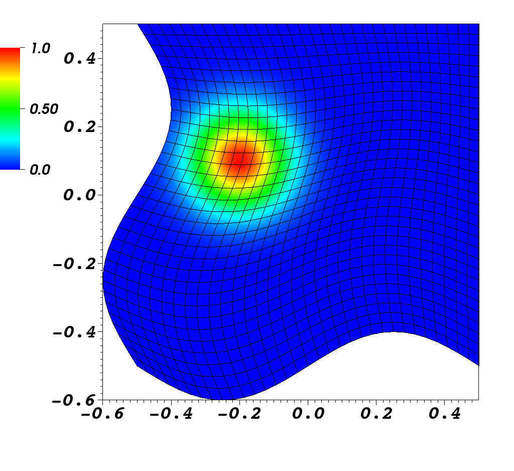
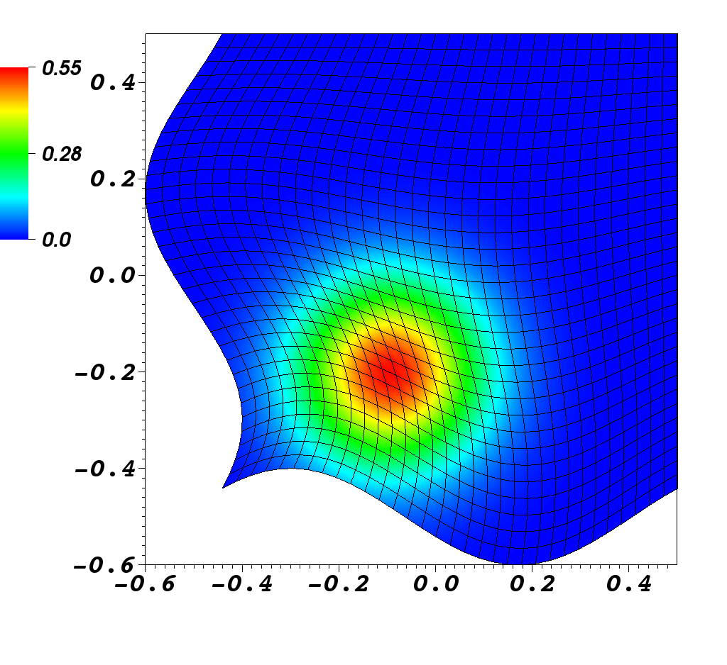
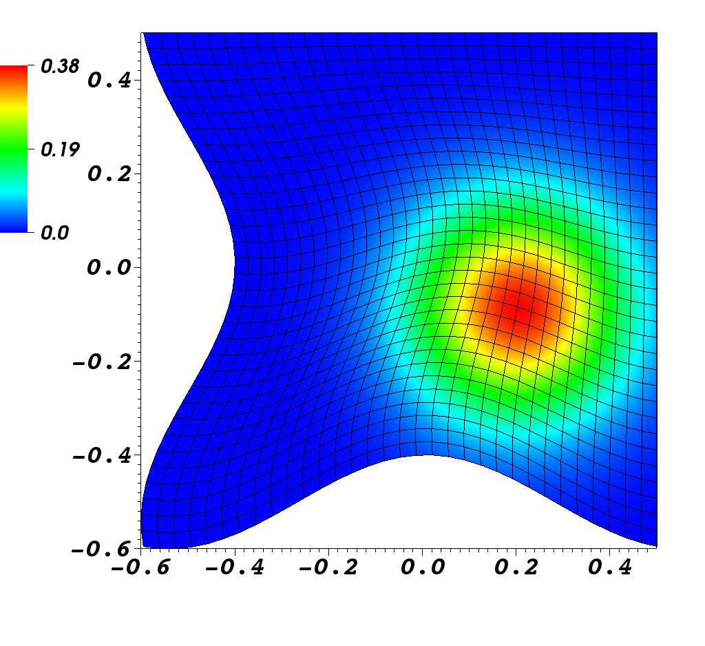
Figure 3: The mesh and solution for $\nu=10^{-2}$ at time levels $t=0,0.4,0.8$ (left to right).

Cells per slab	Nr. of slabs	$p=1$	rates	$p=2$	rates	$p=3$	rates
$64$	$8$	8.00e-2	-	1.52e-2	-	2.87e-3	-
$256$	$16$	3.15e-2	1.3	3.24e-3	2.2	2.92e-4	3.3
$1024$	$32$	1.30e-2	1.3	7.03e-4	2.2	3.21e-5	3.2
$4096$	$64$	5.95e-3	1.1	1.64e-4	2.1	3.80e-6	3.1
$64$	$8$	1.75e-1	-	3.71e-2	-	6.67e-3	-
$256$	$16$	7.78e-2	1.2	6.23e-3	2.6	5.60e-4	3.6
$1024$	$32$	2.51e-2	1.6	1.03e-3	2.6	4.64e-5	3.6
$4096$	$64$	7.60e-3	1.7	1.76e-4	2.5	3.88e-6	3.6

Table 1: Rates of convergence when solving the advection–diffusion problem Eq. 2– Eq. 3 on a time-dependent domain with mesh deformation satisfying Eq. 70 with $\nu=10^{-2}$ (top) and $\nu=10^{-6}$ (bottom).

7 Conclusions

In this paper, we presented and analyzed a space–time hybridizable discontinuous Galerkin method for the advection–diffusion equation on moving domains. We have shown the consistency, boundedness, and stability of the bilinear form, and the well-posedness of the method via an inf-sup condition. Further, we demonstrated the convergence of the method and derived error estimates in a mesh dependent norm. Theory was validated by a numerical example.

References

• [1] MFEM: Modular finite element methods. mfem.org.
• [2] S. C. Brenner and L. R. Scott, The Mathematical Theory of Finite Element Methods, vol. 15 of Texts in Applied Mathematics, Springer, 2008.
• [3] A. Cangiani, Z. Dong, and E. Georgoulis, $hp$-Version space–time discontinuous Galerkin methods for parabolic problems on prismatic meshes, SIAM J. Sci. Comput., 39 (2017), pp. A1251–A1279, http://dx.doi.org/10.1137/16M1073285.
• [4] B. Cockburn, J. Gopalakrishnan, and R. Lazarov, Unified hybridization of discontinuous Galerkin, mixed, and continuous Galerkin methods for second order elliptic problems, SIAM J. Numer. Anal., 47 (2009), pp. 1319–1365, http://dx.doi.org/10.1137/070706616.
• [5] D. A. Di Pietro and A. Ern, Mathematical Aspects of Discontinuous Galerkin Methods, vol. 69 of Mathématiques et Applications, Springer–Verlag Berlin Heidelberg, 2012.
• [6] M. Feistauer, J. Hájek, and K. Švadlenka, Space-time discontinuos Galerkin method for solving nonstationary convection-diffusion-reaction problems, Appl. Math., 52 (2007), pp. 197–233, https://doi.org/10.1007/s10492-007-0011-8.
• [7] M. Feistauer, V. Kučera, K. Najzar, and J. Prokopová, Analysis of space–time discontinuous Galerkin method for nonlinear convection–diffusion problems, Numer. Math., 117 (2011), pp. 251–288, https://doi.org/10.1007/s00211-010-0348-x.
• [8] E. Georgoulis, Discontinuous Galerkin methods on shape-regular and anisotropic meshes, D.Phil. Thesis, University of Oxford, 2003.
• [9] P. Jamet, Galerkin–type approximations which are discontinuous in time for parabolic equations in a variable domain, SIAM J. Numer. Anal., 15 (1978), pp. 912–928, https://doi.org/10.1137/0715059.
• [10] M. Lesoinne and C. Farhat, Geometric conservation laws for flow problems with moving boundaries and deformable meshes, and their impact on aeroelastic computations, Comput. Methods. Appl. Mech. Engrg., 134 (1996), pp. 71–90, http://dx.doi.org/10.1016/0045-7825(96)01028-6.
• [11] A. Masud and T. Hughes, A space-time Galerkin/least–squares finite element formulation of the Navier–Stokes equations for moving domain problems, Comput. Methods Appl. Mech. Engrg., 146 (1997), pp. 91–126, https://doi.org/10.1016/S0045-7825(96)01222-4.
• [12] E. McDonald, J. Pestana, and A. Wathen, Preconditioning and iterative solution of all-at-once systems for evolutionary partial differential equations, SIAM J. Sci. Comput., 40 (2018), pp. A1012–A1033, https://doi.org/10.1137/16M1062016.
• [13] M. Neumüller, Space–time methods: fast solvers and applications, Dissertation, Graz University of Technology, 2013.
• [14] P.-O. Persson, J. Bonet, and J. Peraire, Discontinuous Galerkin solution of the Navier–Stokes equations on deformable domains, Comput. Methods. Appl. Mech. Engrg., 198 (2009), pp. 1585–1595, https://doi.org/10.1016/j.cma.2009.01.012.
• [15] S. Rhebergen and B. Cockburn, A space–time hybridizable discontinuous Galerkin method for incompressible flows on deforming domains, J. Comput. Phys., 231 (2012), pp. 4185–4204, http://dx.doi.org/10.1016/j.jcp.2012.02.011.
• [16] S. Rhebergen and B. Cockburn, Space–time hybridizable discontinuous Galerkin method for the advection–diffusion equation on moving and deforming meshes, in The Courant–Friedrichs–Lewy (CFL) condition, 80 years after its discovery, C. de Moura and C. Kubrusly, eds., Birkhäuser Science, 2013, pp. 45–63, http://dx.doi.org/10.1007/978-0-8176-8394-8_4.
• [17] S. Rhebergen, B. Cockburn, and J. van der Vegt, A space–time discontinuous Galerkin method for the incompressible Navier–Stokes equations, J. Comput. Phys., 233 (2013), pp. 339–358, https://doi.org/10.1016/j.jcp.2012.08.052.
• [18] J. Sudirham, Space–time discontinuous Galerkin methods for convection-diffusion problems, PhD thesis, University of Twente, 2005.
• [19] J. Sudirham, J. van der Vegt, and R. van Damme, Space–time discontinuous Galerkin method for advection–diffusion problems on time-dependent domains, Appl. Numer. Math, 56 (2006), pp. 1491–1518, http://dx.doi.org/10.1016/j.apnum.2005.11.003.
• [20] J. van der Vegt and J. Sudirham, A space–time discontinuous Galerkin method for the time-dependent Oseen equations, Appl. Numer. Math, 58 (2008), pp. 1892–1917, http://dx.doi.org/10.1016/j.apnum.2007.11.010.
• [21] J. van der Vegt and H. van der Ven, Space–time discontinuous Galerkin finite element method with dynamic grid motion for inviscid compressible flows: I. General formulation, J. Comput. Phys., 182 (2002), pp. 546–585, http://doi.org/10.1006/jcph.2002.7185.
• [22] G. N. Wells, Analysis of an interface stabilized finite element method: the advection-diffusion-reaction equation, SIAM J. Numer. Anal., 49 (2011), pp. 87–109, http://doi.org/10.1137/090775464.