NLO Effects in EFT Fits to $W^{+}W^{-}$ Production at the LHC

Abstract

We study the impact of anomalous gauge boson and fermion couplings on the production of $W^{+}W^{-}$ pairs at potential future LHC upgrades and estimate the sensitivity at $\sqrt{S}=14$ TeV with $3~{}ab^{-1}$ and $\sqrt{S}=27$ TeV with $15~{}ab^{-1}$. A general technique for including NLO QCD effects in effective field theory (EFT) fits to kinematic distributions is presented, and numerical results are given for $\sqrt{S}=13$ TeV $W^{+}W^{-}$ production. Our method allows fits to anomalous couplings at NLO accuracy in any EFT basis and has been implemented in a publicly available version of the POWHEG-BOX. Analytic expressions for the $K$-factors relevant for $13$ TeV total cross sections are given for the HISZ and Warsaw EFT bases and differential $K$-factors can be obtained using the supplemental material. Our study demonstrates the necessity of including anomalous $Z$- fermion couplings in the extraction of limits on anomalous 3-gauge-boson couplings.

I Introduction

With the discovery of the Higgs boson, and subsequent measurements of its properties at the LHC, the general features of the Standard Model (SM) electroweak theory have been confirmed experimentally Dawson:2018dcd . Measurements of the Higgs couplings and production rates agree with SM predictions at the $10-20\%$ level Khachatryan:2016vau ; Butter:2016cvz ; Aaboud:2017vzb ; Aaboud:2018xdt ; Sirunyan:2018koj and there is no indication of the existence of any new particle at the TeV scale. Going forward, the task is to make comparisons between theory and data at the few percent level. This requires not only high-luminosity LHC running, but also improved theoretical calculations. Furthermore, Higgs physics cannot be studied in isolation, but must be examined in the context of the entire set of SM interactions.

$W^{+}W^{-}$ pair production is an example of a process whose properties are highly restricted by LEP measurements Schael:2013ita , yet still provides relevant information about the Higgs sector from LHC data. The production of $W^{+}W^{-}$ pairs provides a sensitive test of the electroweak gauge structure, since in the SM there are delicate cancellations between contributions from $s-$channel $\gamma$ and $Z$ exchange and $t-$ channel fermion exchange that maintain perturbative unitarity. Deviations from the form of the $\gamma W^{+}W^{-}$ and $ZW^{+}W^{-}$ vertices predicted by the SM spoil the cancellations between contributions that enforce unitarity. These deviations have been studied for decades Duncan:1985vj ; Hagiwara:1986vm , while the importance of non-SM fermion-$Z$ interactions in ensuring unitarity in $W^{+}W^{-}$ pair production has only recently been realized Zhang:2016zsp ; Baglio:2017bfe ; Alves:2018nof ; Grojean:2018dqj .

Beyond the Standard Model (BSM) physics effects in $W^{+}W^{-}$ production can be studied using effective Lagrangian techniques where the new physics is parameterized as an operator expansion in inverse powers of a high scale, $\Lambda$,

$$L_{\rm SMEFT}=L_{\rm SM}+\sum_{i,n}{C_{i}^{(n)}\over\Lambda^{n-4}}O_{i}^{(n)}+\ldots\,$$ (1)

where $O_{i}^{(n)}$ has mass dimension-$n$ and $L_{\rm SM}$ contains the complete SM Lagrangian. The subscript SMEFT denotes the SM Effective Field Theory where the Higgs is assumed to be part of an $SU(2)$ doublet. This approach further assumes that there are no new light degrees of freedom. Neglecting flavor, there are 59 possible operators at dimension-6 Buchmuller:1985jz ; Grzadkowski:2010es , but only a small subset of these contribute to $W^{+}W^{-}$ production. At high energies, the longitudinally polarized contributions to $W^{+}W^{-}$ grow with energy faster than the SM contributions in the presence of BSM physics. This implies that the LHC can put strong constraints on the coefficients of the dimension-$6$ SMEFT operators.

We consistently work with a dimension-$6$ Lagrangian. At dimension-$8$, there are many other possible operators, not only modifying the triple-gauge boson interactions but also new $4-$point $ggW^{+}W^{-}$ interactions Bellm:2016cks . These operators contribute at tree level at order ${\cal O}(1/\Lambda^{4})$ in the EFT and must be included in a study of the dimension-$8$ Lagrangian. However, the study of dimension-$8$ operators is beyond the scope of this work, so that we do not consider operators modifying the partonic cross section $gg\to W^{+}W^{-}$.

The effects of new physics contributions to $W^{+}W^{-}$ gauge boson pair production can be expected to be of the same order of magnitude as QCD corrections, and so these contributions must be included when extracting limits on new physics. QCD effects in the effective field theory can also change the dependence of the experimental kinematic distributions on the coefficients of Eq. (1). The SM QCD corrections to $W^{+}W^{-}$ pair production are known up to NNLO Gehrmann:2014fva ; Grazzini:2016ctr , including the effects of a jet veto Dawson:2016ysj ; Hamilton:2016bfu , and the electroweak corrections exist at NLO Bierweiler:2013dja ; Baglio:2013toa ; Biedermann:2016guo . The SM and dimension-6 $gg$ initial state contributions are formally NNLO and are not included, although at $14$ TeV they increase the cross section by roughly $10\%$ (see e.g. refs. Campbell:2011bn ; Chiesa:2018lcs ). We perform an analysis including QCD corrections Dixon:1998py ; Dixon:1999di at NLO in the SMEFT, along with modifications of both the 3-gauge-boson and fermion couplings, extending our previous study Baglio:2017bfe by including the leptonic decays of the $W$’s. The effects of anomalous 3-gauge boson couplings exist in the POWHEG-BOX framework Melia:2011tj ; Nason:2013ydw , and we add the additional contributions from anomalous fermion couplings. This public tool can be found at http://powhegbox.mib.infn.it and can be used to perform fits to anomalous couplings including NLO QCD and showering effects.

In Section II, we review the basics of the effective field theory framework for $W$ pair production and discuss the effects of NLO QCD in the SMEFT. The determination of NLO QCD effects in a theory with anomalous couplings has typically been done on a case by case basis, or alternatively by allowing one SMEFT coupling at a time to vary. In Section II.2, we present a general method for deriving NLO expressions for the total cross section and for distributions in an SMEFT in terms of a fixed number of sub-amplitudes, which we term ”primitive cross sections”. These results can be used to obtain either total or differential $K$-factors in any SMEFT basis. In Section III, we compare projections for the measurements of anomalous 3-gauge-boson couplings at the high-luminosity LHC with those of a future $27$ TeV collider and demonstrate the critical importance of including anomalous fermion couplings in the fits (see also ref. Biekotter:2018jzu for SMEFT projections in a global fit at a 27 TeV hadron collider). We provide numerical results in Section IV for $K$-factors for the leading lepton $p_{T}$ ($p_{T}^{\ell,lead}$) and $m_{ll}$ distributions for $W^{+}W^{-}\rightarrow e^{\pm}\mu^{\mp}\nu{\overline{\nu}}$ at $13$ TeV as an illustration of our technique, along with analytic results for the total cross section, as functions of arbitrary EFT coefficients.

II Basics

II.1 Effective Gauge and Fermion Interactions

Assuming CP conservation, the most general Lorentz invariant $3-$gauge boson couplings are Gaemers:1978hg ; Hagiwara:1986vm ,

$$\mathcal{L}_{V}=-ig_{WWV}\biggl{[}g_{1}^{V}\left(W^{+}_{\mu\nu}W^{-\mu}V^{\nu}-W_{\mu\nu}^{-}W^{+\mu}V^{\nu}\right)+\kappa^{V}W^{+}_{\mu}W^{-}_{\nu}V^{\mu\nu}+\frac{\lambda^{V}}{M^{2}_{W}}W^{+}_{\rho\mu}{W^{-\mu}}_{\nu}V^{\nu\rho}\biggr{]},$$ (2)

where $V=\gamma,Z$, $g_{WW\gamma}=e$ and $g_{WWZ}=g\cos\theta_{W}$, with $\theta_{W}$ being the weak mixing angle, ($s_{W}\equiv\sin\theta_{W}$, $c_{W}\equiv\cos\theta_{W}$). The fields in Eq.(2) are the canonically normalized mass eigenstate fields. We define $g_{1}^{V}=1+\delta g_{1}^{V}$, $\kappa^{V}=1+\delta\kappa^{V}$ and in the SM $\delta g_{1}^{V}=\delta\kappa^{V}=\lambda^{V}=0$. Gauge invariance requires $\delta g_{1}^{\gamma}=0$.

The effective couplings of quarks to gauge fields can be written as, (assuming no new tensor structures),

$$\mathcal{L} \equiv g_{Z}Z_{\mu}\biggl{[}g_{L}^{Zq}+\delta g_{L}^{Zq}\biggr{]}{\overline{q}}_{L}\gamma_{\mu}q_{L}\ +g_{Z}Z_{\mu}\biggl{[}g_{R}^{Zq}+\delta g_{R}^{Zq}\biggr{]}{\overline{q}}_{R}\gamma_{\mu}q_{R}$$ (3)

$$+{g\over\sqrt{2}}\biggl{\{}W_{\mu}\biggl{[}(1+\delta g_{L}^{W}){\overline{u}}_{L}\gamma_{\mu}d_{L}+\delta g_{R}^{W}{\overline{u}}_{R}\gamma_{\mu}d_{R}\biggr{]}+h.c.\biggr{\}}\,.$$

$g_{Z}=e/(c_{W}s_{W})=g/c_{W}$, $Q_{q}$ is the electric charge of the quarks, and $q$ denotes up-type or down-type quarks. We assume the anomalous fermion couplings, $\delta g_{L,R}^{Zq}$, along with the anomalous $W$ -fermion couplings are flavor independent. We also neglect CKM mixing. The SM quark couplings are:

$$g_{R}^{Zq} = -s_{W}^{2}Q_{q}\quad{\rm and}\quad g_{L}^{Zq}=T_{3}^{q}-s_{W}^{2}Q_{q},$$ (4)

with $T_{3}^{q}=\pm\displaystyle\frac{1}{2}$. $SU(2)$ invariance implies,

$$\delta g_{L}^{W} = \delta g_{L}^{Zu}-\delta g_{L}^{Zd},$$

$$\delta g_{1}^{Z} = \delta\kappa^{Z}+{s_{W}^{2}\over c_{W}^{2}}\delta\kappa^{\gamma},$$

$$\lambda^{\gamma} = \lambda^{Z}\,.$$ (5)

This framework leads to $7$ unknown parameters: $\delta g_{1}^{Z},~{}\delta\kappa_{Z},~{}\lambda_{Z},~{}\delta g_{L}^{Zu},~{}\delta g_{L}^{Zd},~{}\delta g_{R}^{Zu}$ and $~{}\delta g_{R}^{Zd}$.

At high energy scales the dominant contributions to $W^{+}W^{-}$ come from longitudinally polarized $W^{\prime}s$. Keeping only the terms linear in the anomalous couplings, the amplitudes ${{\cal A}}_{rr^{\prime}\lambda\lambda^{\prime}}$ for ${\overline{q}}_{r}q_{r^{\prime}}\rightarrow W^{+}_{\lambda}W^{-}_{\lambda^{\prime}}$, where $r,r^{\prime},\lambda,\lambda^{\prime}$ label the respective particle helicities, have the high energy limits Gaemers:1978hg ; Hagiwara:1986vm ; Azatov:2016sqh ; Falkowski:2016cxu ; Baglio:2017bfe ; Alves:2018nof ; Grojean:2018dqj ,

$${{\cal A}}_{+-00} \rightarrow {g^{2}s\over 2M_{W}^{2}}\sin\theta\biggl{\{}\delta\kappa^{Z}\biggl{(}s_{W}^{2}Q_{q}-T_{3}^{q}\biggr{)}-s_{W}^{2}Q_{q}\delta\kappa^{\gamma}-\delta g_{L}^{Zq}+2T_{3}^{q}\delta g_{L}^{W}\biggr{\}},$$

$${{\cal A}}_{-+00} \rightarrow {g^{2}s\over 2M_{W}^{2}}\sin\theta\biggl{\{}s_{W}^{2}Q_{q}\biggl{(}\delta\kappa^{\gamma}-\delta\kappa^{Z}\biggr{)}+\delta g_{R}^{Zq}\biggr{\}}\,,$$ (6)

where $\sqrt{s}$ is the partonic sub-energy. From Eq.(6), it is clear that the longitudinal polarizations do not depend on the full range of $7$ anomalous couplings, but on 4 linear combinations when $u$ and $d$ contributions are included. Note that the dependence on $\lambda_{Z}$ is subleading in $s$. The transverse polarizations have a weaker dependence on the energy scale and different dependences on the anomalous couplings.

The Lagrangians of Eqs.(2) and (3) can be mapped onto the effective Lagrangian of Eq.(1). For future convenience, we consider the mapping to the Warsaw basis Grzadkowski:2010es ; Dedes:2017zog and the HISZ basis Hagiwara:1986vm . In the Warsaw basis Grzadkowski:2010es , the dimension-$6$ operators relevant for our analysis are,

$$L_{WARSAW} = {C_{3W}\over\Lambda^{2}}\epsilon^{abc}W_{\mu}^{a\nu}W_{\nu}^{b\rho}W_{\rho}^{c\mu}+{C_{HD}\over\Lambda^{2}}\mid\Phi^{\dagger}(D_{\mu}\Phi)\mid^{2}+{C_{HWB}\over\Lambda^{2}}\Phi^{\dagger}\sigma^{a}\Phi W^{a}_{\mu\nu}B^{\mu\nu}$$ (7)

$$+{C_{Hf}^{(3)}\over\Lambda^{2}}i\biggl{(}\Phi^{\dagger}\overleftrightarrow{D}_{\mu}^{a}\Phi\biggr{)}{\overline{f}}_{L}\gamma^{\mu}\sigma^{a}f_{L}+{C_{Hf}^{(1)}\over\Lambda^{2}}i\biggl{(}\Phi^{\dagger}\overleftrightarrow{D}_{\mu}\Phi\biggr{)}{\overline{f}}_{L}\gamma^{\mu}f_{L}$$

$$+{C_{Hf}\over\Lambda^{2}}i\biggl{(}\Phi^{\dagger}\overleftrightarrow{D}_{\mu}\Phi\biggr{)}{\overline{q}}_{R}\gamma^{\mu}q_{R}+{C_{Hud}\over\Lambda^{2}}i\biggl{(}\widetilde{\Phi}^{\dagger}D_{\mu}\Phi\biggr{)}\overline{u}_{R}\gamma^{\mu}d_{R}$$

$$+{C_{ll}\over\Lambda^{2}}({\overline{l}}_{L}\gamma^{\mu}l_{L})({\overline{l}}_{L}\gamma_{\mu}l_{L})\,,$$

where $f$ can be either a quark or a lepton, $D_{\mu}\Phi=(\partial_{\mu}-i\,\frac{g}{2}\sigma^{a}W^{a}_{\mu}-i\frac{g^{\prime}}{2}B_{\mu})\Phi$, $W^{a}_{\mu\nu}=\partial_{\mu}W^{a}_{\nu}-\partial_{\nu}W^{a}_{\mu}+g\varepsilon^{abc}W^{b}_{\mu}W^{c}_{\nu}$, $\Phi^{\dagger}\overleftrightarrow{D}_{\mu}\Phi=\Phi^{\dagger}D_{\mu}\Phi-(D_{\mu}\Phi^{\dagger})\Phi$, and $\Phi^{\dagger}\overleftrightarrow{D}^{a}_{\mu}\Phi=\Phi^{\dagger}D_{\mu}\sigma^{a}\Phi-(D_{\mu}\Phi^{\dagger})\sigma^{a}\Phi$. $\Phi$ stands for the Higgs doublet field with a vacuum expectation value $\langle\Phi\rangle=(0,v/\sqrt{2})^{\rm T}$.

In the HISZ basis, the fermion couplings are unchanged, while the 3-gauge-boson couplings are,

$$L_{HISZ} = {f_{W}\over\Lambda^{2}}(D_{\mu}\Phi)^{\dagger}{\hat{W}}^{\mu\nu}D_{\nu}\Phi+{f_{B}\over\Lambda^{2}}(D_{\mu}\Phi)^{\dagger}{\hat{B}}^{\mu\nu}D_{\nu}\Phi+{f_{WWW}\over\Lambda^{2}}Tr\biggl{(}{\hat{W}}_{\mu\nu}{\hat{W}}^{\nu\rho}{\hat{W}}_{\rho}^{\mu}\biggr{)}\,,$$ (8)

where ${\hat{W}}^{\mu\nu}=i{g\over 2}\sigma^{a}W^{a,\mu\nu}$ and ${\hat{B}}^{\mu\nu}=i{g^{\prime}\over 2}B^{\mu\nu}$. Expressions for the anomalous 3-gauge-boson couplings are given in Table 1 and for the anomalous fermion couplings in Table  2.

	Warsaw Basis	HISZ
$\delta g_{1}^{Z}$	$\frac{v^{2}}{\Lambda^{2}}\frac{1}{c_{W}^{2}-s_{W}^{2}}\left(\frac{s_{W}}{c_{W}}C_{HWB}+\frac{1}{4}C_{HD}+\delta v\right)$	${M_{Z}^{2}\over 2\Lambda^{2}}f_{W}$
$\delta\kappa^{Z}$	$\frac{v^{2}}{\Lambda^{2}}\frac{1}{c_{W}^{2}-s_{W}^{2}}\left(2s_{W}c_{W}C_{HWB}+\frac{1}{4}C_{HD}+\delta v\right)$	${M_{Z}^{2}\over 2\Lambda^{2}}(c_{W}^{2}f_{W}-s_{W}^{2}f_{B})$
$\delta\kappa^{\gamma}$	$-\frac{v^{2}}{\Lambda^{2}}\frac{c_{W}}{s_{W}}C_{HWB}$	${M_{W}^{2}\over 2\Lambda^{2}}(f_{W}+f_{B})$
$\lambda^{\gamma}$	$\frac{v}{\Lambda^{2}}3M_{W}C_{3W}$	${3g^{2}M_{W}^{2}\over 4\Lambda^{2}}f_{WWW}$
$\lambda^{Z}$	$\frac{v}{\Lambda^{2}}3M_{W}C_{3W}$	${3g^{2}M_{W}^{2}\over 4\Lambda^{2}}f_{WWW}$

Table 1: Anomalous 3-gauge-boson couplings in the Warsaw Grzadkowski:2010es and HISZ Hagiwara:1986vm . $\delta v$ is given in Table 2.

	Warsaw Basis
$\delta g_{L}^{Zu}$	$-\frac{v^{2}}{2\Lambda^{2}}\left(C_{Hq}^{(1)}-C_{Hq}^{(3)}\right)+\frac{1}{2}\delta g_{Z}+\frac{2}{3}\left(\delta s_{W}^{2}-s_{W}^{2}\delta g_{Z}\right)$
$\delta g_{L}^{Zd}$	$-\frac{v^{2}}{2\Lambda^{2}}\left(C_{Hq}^{(1)}+C_{Hq}^{(3)}\right)-\frac{1}{2}\delta g_{Z}-\frac{1}{3}\left(\delta s_{W}^{2}-s_{W}^{2}\delta g_{Z}\right)$
$\delta g_{R}^{Zu}$	$-\frac{v^{2}}{2\Lambda^{2}}C_{Hu}+\frac{2}{3}\left(\delta s_{W}^{2}-s_{W}^{2}\delta g_{Z}\right)$
$\delta g_{R}^{Zd}$	$-\frac{v^{2}}{2\Lambda^{2}}C_{Hd}-\frac{1}{3}\left(\delta s_{W}^{2}-s_{W}^{2}\delta g_{Z}\right)$
$\delta g_{L}^{W}$	$\frac{v^{2}}{\Lambda^{2}}C_{Hq}^{(3)}+c_{W}^{2}\delta g_{Z}+\delta s_{W}^{2}$
$\delta g_{Z}$	$-\frac{v^{2}}{\Lambda^{2}}\left(\delta v+\frac{1}{4}C_{HD}\right)$
$\delta v$	$C_{Hl}^{(3)}-\frac{1}{2}C_{ll}$
$\delta s_{W}^{2}$	$-\frac{v^{2}}{\Lambda^{2}}\frac{s_{W}c_{W}}{c_{W}^{2}-s_{W}^{2}}\left[2s_{W}c_{W}\left(\delta v+\frac{1}{4}C_{HD}\right)+C_{HWB}\right]$

Table 2: Anomalous fermion couplings in the Warsaw Grzadkowski:2010es basis.

II.2 Primitive Cross Sections

We want to compute differential and total cross sections for a hadronic scattering process at NLO QCD for arbitrary anomalous couplings. Since these calculations can be numerically intensive, it is desirable not to have to repeat the calculation over and over again for different values of the anomalous couplings. Here we discuss a technique for generating results in terms of a set of primitive cross sections which need to be calculated only once for a given process and set of cuts. The primitive cross sections can be reweighted to allow for rapid scans over the anomalous couplings at NLO order.

Consider an arbitrary differential cross section $d\sigma^{n}({\vec{C}})$ that is calculated to ${\cal O}({\Lambda^{-2n}})$. It depends on $m$ EFT coefficients $\vec{C}=(C_{1},C_{2},\ldots,C_{m})$ and the relevant momenta, ${\vec{p}}$. We assume $C_{i}\sim{\cal{O}}({\Lambda^{-2}})$. It is important to note that in general $d\sigma^{4}$ is the cross section to order $\mathcal{O}({\Lambda^{-4}})$, but is not the amplitude-squared. When both $Z-$ fermion and three gauge boson (3GB) couplings are non-zero, the amplitude-squared contains terms up to ${\cal{O}}({\Lambda^{-8}})$.

Calculating the cross section to ${\cal O}({\Lambda^{-2}})$,

$$d\sigma^{1}({\vec{C}})\equiv d\sigma_{SM}(1-\Sigma_{i=1}^{m}C_{i})+\Sigma_{i=1}^{m}C_{i}\,d\sigma(1;{\vec{R}}_{i})\,,$$ (9)

where $\vec{R}_{i}$ are $m$- dimensional vectors with $\vec{R}_{1}=(1,0,0.....0)$, $\vec{R}_{2}=(0,1,0....)$, $\vec{R}_{m}=(0,0....1)$, etc. The primitive cross section $d\sigma(n;\vec{R}_{i})$ is the cross section obtained to arbitrary order ${\cal{O}}({\Lambda^{-2n}})$ when $C_{i}=1$ and all other $C_{j}=0$, $j\neq i$:

$$d\sigma(n;\vec{R}_{i})\equiv d\sigma^{n}(\vec{C}=\vec{R}_{i}).$$ (10)

The SM cross section with $\vec{C}=0$ is $d\sigma_{SM}$. For the process $pp\rightarrow W^{+}W^{-}$ under consideration here, there are 7 primitive cross sections, $d\sigma(1;\vec{R}_{i})$, when considering both anomalous 3GB couplings and anomalous $Z-$fermion couplings, while there are only 3 when the fermion couplings take their SM values. Eq.(9) holds bin by bin for differential rates and also for the total rate.

The procedure becomes significantly more laborious if the cross section is computed to ${\cal{O}}({\Lambda^{-4}})$. We define an $m$-dimensional vectors ${\vec{M}}_{ij}$, with $\vec{M}_{12}=(1,1,0,...0)$, $\vec{M}_{13}=(1,0,1....0)$, $\vec{M}_{23}=(0,1,1,....)$, etc. To ${\cal O}({\Lambda^{-4}})$, the cross section decomposes into the primitive cross sections as,

$$d\sigma^{2}({\vec{C}}) = d\sigma_{SM}(1-\Sigma_{i=1}^{m}C_{i})+\Sigma_{i}C_{i}\,d\sigma(1;{\vec{R}}_{i})+\Sigma_{i=1}^{m}C_{i}^{2}\,\biggl{(}d\sigma(2;{\vec{R}}_{i})-d\sigma(1;{\vec{R}}_{i})\biggr{)}$$ (11)

$$+\Sigma_{i>j=1}^{m}C_{i}C_{j}\biggl{[}d\sigma(2;\vec{M}_{ij})-d\sigma(2;{\vec{R}}_{i})-d\sigma(2;{\vec{R}}_{j})+d\sigma_{SM}\biggr{]}\,.$$

Evaluating the cross section with $2$ non-zero $C_{i}$ coefficients, $C_{i}=1$, $C_{j}=1$, and $C_{k\ell}=0$ if $j\neq i$ or $k\neq\ell$, to arbitrary order $\mathcal{O}(\Lambda^{-2n})$ yields the primitive cross sections

$$d\sigma(n;\vec{M}_{ij})\equiv d\sigma^{n}(\vec{C}=\vec{M}_{ij}).$$ (12)

We can calculate the primitive cross sections, $d\sigma(n;{\vec{R}_{i}})$ and $d\sigma(n;{\vec{M}_{ij}})$ once and then apply Eq.(11) to get the general result for arbitrary anomalous couplings. Eqs.(9) and (11) hold separately for LO and NLO corrected rates. For $pp\rightarrow W^{+}W^{-}$, there are 35 primitive cross sections at ${\cal{O}}({\Lambda^{-4}})$ with both anomalous 3GB couplings and anomalous fermion couplings non-zero.

Suppose we calculate the primitive cross sections in terms of a set of EFT parameters, $\vec{C}=(C_{1},\ldots,C_{m})$, but we want the results in terms of a different EFT basis, $\vec{C}^{\prime}=(C_{1}^{\prime},\ldots,C_{m}^{\prime})$. The procedure is straightforward. We begin by considering $2$ anomalous couplings, $m=2$, and the $\mathcal{O}(\Lambda^{-2})$ case. The physical rate must be independent of the basis choice and using the master formula of Eq.(9) for the $2$ different bases,

$$d\sigma^{1}({\vec{C}}) = d\sigma_{SM}(1-C_{1}-C_{2})+C_{1}\,d\sigma(1;\vec{R}_{1})+C_{2}\,d\sigma(1;\vec{R}_{2})$$

$$d\sigma^{1}({\vec{C^{\prime}}}) = d\sigma_{SM}(1-C_{1}^{\prime}-C_{2}^{\prime})+C_{1}^{\prime}\,d\sigma^{\prime}(1;\vec{R}_{1})+C_{2}^{\prime}\,d\sigma^{\prime}(1;\vec{R}_{2}).$$ (13)

The unprimed primitive cross sections are defined according to Eq.(10). To order $\mathcal{O}(\Lambda^{-2n})$ the primed primitive cross sections $d\sigma^{\prime}(n,\vec{R}_{i}\prime)$ are defined with the vector $\vec{R}_{i}$ evaluated relative to the new basis $\vec{C}^{\prime}$

$$d\sigma^{\prime}(n;\vec{R}_{i})\equiv d\sigma^{n}(\vec{C^{\prime}} = \vec{R}_{i}).$$ (14)

We need the $d\sigma^{\prime}$’s in terms of the already computed $d\sigma$’s so that we can avoid recalculating the cross sections. Including a complete basis of dimension-6 operators, the input parameters are related by a linear transformation,

$$\left(\begin{array}[]{c}C_{1}\\ C_{2}\\ \end{array}\right)=\alpha\left(\begin{array}[]{c}C_{1}^{\prime}\\ C_{2}^{\prime}\\ \end{array}\right)\,,$$ (15)

where $\alpha$ is a $2\times 2$ matrix. The $d\sigma^{\prime}$ matrices are:

$$d\sigma^{\prime}(1;\vec{R}_{1}) = d\sigma_{SM}(1-\alpha_{11}-\alpha_{21})+\alpha_{11}\,d\sigma(1;\vec{R}_{1})+\alpha_{21}\,d\sigma(1;\vec{R}_{2})$$ (16)

$$d\sigma^{\prime}(1;\vec{R}_{2}) = d\sigma_{SM}(1-\alpha_{12}-\alpha_{22})+\alpha_{12}\,d\sigma(1;\vec{R}_{1})+\alpha_{22}\,d\sigma(2;\vec{R}_{2})\,.$$ (17)

Now consider the general case of a change of EFT input basis. Assume we have two minimum sets of independent parameters $\vec{C}=(C_{1},C_{2},\cdots,C_{m})$ and $\vec{C^{\prime}}=(C^{\prime}_{1},C^{\prime}_{2},\cdots,C^{\prime}_{m})$ that can be related linearly,

$$C_{i}=\sum_{j=1}^{m}\alpha_{ij}C_{j}^{\prime},\quad C_{i}^{\prime}=\sum_{j=1}^{m}\alpha^{-1}_{ij}C_{j},$$ (18)

where $\alpha^{-1}$ is the inverse matrix of $\alpha$ and $\alpha^{-1}_{ij}$ is its $\{i,j\}^{th}$ element.

Although the two parameter bases $C_{i},C^{\prime}_{i}$ must give identical results for physical quantities and,

$$\sigma^{n}\equiv\sigma^{n}(\vec{C})=\sigma^{n}(\vec{C^{\prime}})\,,$$ (19)

the primitive cross sections are not the same since setting $C_{i}=1$ is not the same as taking $C^{\prime}_{i}=1$. To $\mathcal{O}(\Lambda^{-2n})$, we define the primitive cross sections with two non-zero $C^{\prime}_{j}$ in the $\vec{C}^{\prime}$ bases to be

$$d\sigma^{\prime}(2;\vec{M}_{ij})\equiv d\sigma^{n}(\vec{C^{\prime}}=\vec{M}_{ij}^{\prime})\,$$ (20)

where $\vec{M}_{ij}$ evaluated relative to the $\vec{C}$ basis. The primitive cross sections $d\sigma(n;\vec{R}_{i})$, $d\sigma(n;\vec{M}_{ij})$, and $d\sigma^{\prime}(n;\vec{R}_{j})$ are defined in Eqs.(10), (12), and (14), respectively.

The cross sections can now be expanded in terms of either set of parameters and primitive cross sections. At $\mathcal{O}(\Lambda^{-2})$, we have the cross sections

$$d\sigma^{1} = d\sigma_{SM}+\sum_{i=1}^{m}C_{i}\left(d\sigma(1;\vec{R}_{i})-d\sigma_{SM}\right)$$ (21)

$$= d\sigma_{SM}+\sum_{i=1}^{m}C^{\prime}_{i}\left(d\sigma^{\prime}(1;\vec{R}_{i})-d\sigma_{SM}\right),$$

where $\sigma_{SM}$ is the SM cross section with $\vec{C}=\vec{C^{\prime}}=\vec{0}$. At order $\mathcal{O}(\Lambda^{-4})$, we have

$$d\sigma^{2} = d\sigma_{SM}+\sum_{i=1}^{m}C_{i}\left(d\sigma(1;\vec{R}_{i})-d\sigma_{SM}\right)+\sum_{i=1}^{m}C_{i}^{2}\left(d\sigma(2;\vec{R}_{i})-d\sigma(1;\vec{R}_{i})\right)$$ (22)

$$+\Sigma_{i>j=1}^{m}C_{i}C_{j}\left(d\sigma(2;\vec{M}_{ij})-d\sigma(2;\vec{R}_{i})-d\sigma(2;\vec{R}_{j})+d\sigma_{SM}\right)$$

$$= d\sigma_{SM}+\sum_{i=1}^{m}C^{\prime}_{i}\left(d\sigma^{\prime}(1;\vec{R}_{i})-d\sigma_{SM}\right)+\sum_{i=1}^{m}{C^{\prime}}_{i}^{2}\left(d\sigma^{\prime}(2;\vec{R}_{i})-d\sigma^{\prime}(1;\vec{R}_{i})\right)$$

$$+\Sigma_{i>j=1}^{m}C^{\prime}_{i}C^{\prime}_{j}\left(d\sigma^{\prime}(2;\vec{M}_{ij})-d\sigma^{\prime}(2;\vec{R}_{i})-d\sigma^{\prime}(2;\vec{R}_{j})+d\sigma_{SM}\right)\,.$$

Finally, we find the relationships between the primitive cross sections using Eqs. (18,21,22) that can be used to calculate cross sections in terms of an arbitrary EFT basis:

$$d\sigma^{\prime}(1;\vec{R}_{i}) = d\sigma_{SM}+\sum_{k=1}^{m}\alpha_{ki}\left(d\sigma(1;\vec{R}_{k})-d\sigma_{SM}\right)$$

$$d\sigma^{\prime}(2;\vec{R}_{i}) = d\sigma^{\prime}(1;\vec{R}_{i})+\sum_{k=1}^{m}\alpha_{ki}^{2}\left(d\sigma(2;\vec{R}_{k})-d\sigma(1;\vec{R}_{k})\right)$$

$$+ \sum_{k>l=1}^{m}\alpha_{ki}\alpha_{li}\left(d\sigma(2;\vec{M}_{kl})-d\sigma(2;\vec{R}_{k})-d\sigma(2;\vec{R}_{l})+d\sigma_{SM}\right)$$

$$d\sigma^{\prime}(2;\vec{M}_{ij}) = d\sigma^{\prime}(1;\vec{R}_{i})+d\sigma^{\prime}(1;\vec{R}_{j})-d\sigma_{SM}$$

$$+ \sum_{k=1}^{m}\left(\alpha_{ki}+\alpha_{kj}\right)^{2}\left(d\sigma(2;\vec{R}_{k})-d\sigma(1;\vec{R}_{k})\right)$$

$$+ \sum_{k>l=1}^{m}\left(\alpha_{ki}+\alpha_{kj}\right)\left(\alpha_{li}+\alpha_{lj}\right)(d\sigma(2;\vec{M}_{kl})-d\sigma(2;\vec{R}_{k})-d\sigma(2;\vec{R}_{l})+d\sigma_{SM})\,,$$

or equivalently,

$$d\sigma(1;\vec{R}_{i}) = d\sigma_{SM}+\sum_{k=1}^{m}\alpha^{-1}_{ki}\left(d\sigma^{\prime}(1;\vec{R}_{k})-d\sigma_{SM}\right)$$

$$d\sigma(2;\vec{R}_{i}) = d\sigma(1;\vec{R}_{i})+\sum_{k=1}^{m}(\alpha_{ki}^{-1})^{2}\left(d\sigma^{\prime}(2;\vec{R}_{k})-d\sigma^{\prime}(1;\vec{R}_{k})\right)$$

$$+ \sum_{k>l=1}^{m}\alpha^{-1}_{ki}\alpha^{-1}_{li}\left(d\sigma^{\prime}(2;\vec{M}_{kl})-d\sigma^{\prime}(2;\vec{R}_{k})-d\sigma^{\prime}(2;\vec{R}_{l})+d\sigma_{SM}\right)$$

$$d\sigma(2;\vec{M}_{ij}) = d\sigma(1;\vec{R}_{i})+d\sigma(1;\vec{R}_{j})-d\sigma_{SM}$$

$$+ \sum_{k=1}^{m}\left(\alpha^{-1}_{ki}+\alpha^{-1}_{kj}\right)^{2}\left(d\sigma^{\prime}(2;\vec{R}_{k})-d\sigma^{\prime}(1;\vec{R}_{k})\right)$$

$$+ \sum_{k>l=1}^{m}\left(\alpha^{-1}_{ki}+\alpha^{-1}_{kj}\right)\left(\alpha^{-1}_{li}+\alpha^{-1}_{lj}\right)\left(d\sigma^{\prime}(2;\vec{M}_{kl})-d\sigma^{\prime}(2;\vec{R}_{k})-d\sigma^{\prime}(2;\vec{R}_{l})+d\sigma_{SM}\right)\,.$$

The above results are found using

$$C_{i}C_{j}=\sum_{k=1}^{m}\alpha_{ik}\alpha_{jk}{C^{\prime}_{k}}^{2}+\sum_{k>l=1}^{m}\left(\alpha_{ik}\alpha_{jl}+\alpha_{il}\alpha_{jk}\right)C^{\prime}_{k}C^{\prime}_{l},$$ (24)

which simplifies for $i=j$

$${C}_{i}^{2}=\sum_{k=1}^{m}\alpha^{2}_{ik}{C^{\prime}}^{2}_{k}+2\sum_{k>l=1}^{m}\alpha_{ik}\alpha_{il}C^{\prime}_{k}C^{\prime}_{l}.$$ (25)

We illustrate the procedure and the utility of the results in this section by transforming from the Warsaw to HISZ basis in Sec. IV.

III Future Projections

In this section, we apply the results of the previous sections to projecting allowed regions for anomalous 3-gauge-boson and $Z-$fermion couplings at a high-luminosity LHC (HL-LHC) and a potential $27$ TeV collider (HE-LHC) under various assumptions about the systematic uncertainties We have extended the POWHEG-BOX-V2 Nason:2004rx ; Frixione:2007vw ; Alioli:2010xd implementation of the NLO QCD corrected predictions for the process $pp\to W^{+}W^{-}\to 4\ell$ Melia:2011tj ; Nason:2013ydw , that contains only the 3-gauge-boson anomalous couplings, as originally found in Refs. Dixon:1998py ; Dixon:1999di and implemented also in MCFM Campbell:1999ah . In our implementation in the POWHEG-BOX-V2, we also include the anomalous Z-fermion couplings, there is the option to choose the order of the $\Lambda^{-2n}$ expansion and the results can be generated using the effective interactions of Eqs.(2) and (3) or the Warsaw basis coefficients of Eq.(7). Our projections assume the $\Lambda^{-4}$ expansion. Note that our extension works for the case of different-flavor leptonic final states. In the case of same-flavor charged leptons the contribution from $ZZ$ production as well as the interference between $W^{+}W^{-}$ and $ZZ$ contributions should be included.

We apply the basic cuts,

$$p_{T}^{\ell}>30~{}{\rm GeV},\,|\eta^{\ell}|<2.5,\,m_{\ell\ell}>10~{}{\rm GeV},\,\not{E}_{T}>20~{}{\rm GeV},\ell=e^{\pm},\mu^{\mp}\,,$$ (26)

where $p_{T}^{\ell}$ is charged lepton transverse momentum, $\eta^{\ell}$ is charged lepton rapidity, $m_{\ell\ell}$ is the invariant mass of the two charged leptons, and $\not{E}_{T}$ is the missing energy of the event. Since we do not include detector effects, in our case the missing transverse energy is the transverse energy of the two final state neutrinos. We work at the parton level and veto jets with

$$p_{T}^{jet}>35~{}{\rm GeV},\,|\eta^{jet}|<4.5\,,$$ (27)

where $p_{T}^{jet}$ is the jet transverse momentum and $\eta^{jet}$ is the jet rapidity. We further assume a $50\%$ efficiency, in line with the experimental results of Ref. Aad:2016wpd . We use CT14QED Inclusive PDFs Schmidt:2015zda , and take the renormalization/factorization scales equal to $\displaystyle{M_{WW}\over 2}$.

We assume a systematic uncertainty of $\delta_{syst}=16\%$ and find the point where the systematic and statistical errors on the leading lepton $p_{T}$ distribution are roughly equal, $\delta_{stat}\sim\delta_{sys}$. At this point, the uncertainties are systematics dominated and increased statistics provide diminishing returns. (In our figures, we investigate the impact of reducing the systematic error to $\delta_{syst}=4\%$.) We define this point in terms of the integral over the leading lepton transverse momentum $p_{T}^{\ell,lead}$ above a cut $p_{T,cut}$,

$$\sigma(p_{T}^{\ell,lead}>p_{T,cut})=\int_{p_{T,cut}}\frac{d\sigma}{dp_{T}^{\ell,lead}}dp_{T}^{\ell,lead}\,.$$ (28)

The $p_{T}$ cut is defined to be the point where,

$$\delta_{sys}=\delta_{stat}=\frac{1}{\sqrt{N}}=\frac{1}{\sqrt{L\sigma(p_{T}^{\ell,lead}>p_{T,cut})}}$$ (29)

$$\Rightarrow \sigma(p_{T}^{\ell,lead}>p_{T,cut})=\frac{1}{L\delta^{2}_{sys}}.$$

$L$ is the integrated luminosity and $N$ is the number of events passing the cuts. This corresponds to roughly $38$ events above the cut. Using integrated luminosities of $3~{}fb^{-1}$ at $14$ TeV and $15~{}fb^{-1}$ at $27$ TeV, we determine the $p_{T}$ cuts:

$$14~{}\text{TeV}:~{}p_{T,cut} = 750~{}GeV$$

$$27~{}\text{TeV}:~{}p_{T,cut} = 1350~{}GeV\,.$$ (30)

Retaining $\delta_{stat}=16\%$ with the corresponding $p_{T}$ cuts of Eq.(30), we also consider the effect of reducing the systematic error to $\delta_{sys}=4\%$.

We begin by setting the fermion couplings to their SM values. In this case the expansion to $\mathcal{O}(\Lambda^{-4})$ is the full amplitude-squared, including both SM and SMEFT contributions. The projections at NLO QCD for $14$ TeV are shown in Fig. 1 and for $27$ TeV in Fig. 2, in black for $\delta_{sys}=16\%$ and in red for $\delta_{sys}=4\%$, named “3GB”. We see a significant improvement going from $14$ TeV to $27$ TeV, while the improvement from reducing the systematic error, $\delta_{sys}=16\%\to 4\%$, is marginal. Compared to Ref. Baglio:2017bfe , the improvement from $8$ TeV to HL-LHC and HE-LHC is important. The coefficient $\lambda^{Z}$ in particular is highly constrained, $|\lambda^{Z}|<2\times 10^{-3}$ at the HL-LHC and improved to $|\lambda^{Z}|<6\times 10^{-4}$ at the HE-LHC.

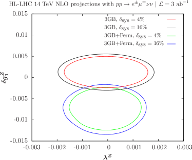
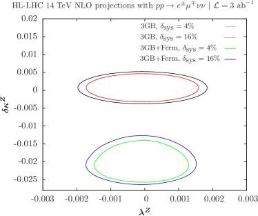
Figure 1: Projections for the $14$ TeV HE-LHC with $3~{}ab^{-1}$. We take $p_{T,cut}=750$ GeV, corresponding to $\delta_{stat}=16\%$ and consider $\delta_{sys}=16\%$ and $\delta_{sys}=4\%$. The curves labeled “3GB” have SM $Z-$fermion couplings (black and red), while the curves labeled “3GB+Ferm” allow the fermion couplings to vary within the $2\sigma$ region defined by Eq.(31) (blue and green). The standard cuts given in Eqs. (26) and (27) are applied.

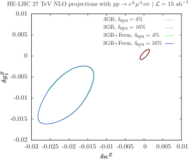
Figure 2: Projections for the $27$ TeV HE-LHC with $15~{}ab^{-1}$.We take $p_{T,cut}=1350$ GeV, corresponding to $\delta_{stat}=16\%$ and consider $\delta_{sys}=16\%$ and $\delta_{sys}=4\%$. The curves labeled “3GB” have SM $Z-$fermion couplings (black and red), while the curves labeled “3GB+Ferm” allow the fermion couplings to vary within the $2\sigma$ region defined by Eq.(31) (blue and green). The standard cuts given in Eqs. (26) and (27) are applied.

As demonstrated in Refs. Baglio:2017bfe ; Grojean:2018dqj ; Alves:2018nof ; Liu:2018pkg ; Falkowski:2016cxu , anomalous fermion couplings can have similar effects on the $W^{+}W^{-}$ distributions as do the anomalous 3-gauge-boson couplings. At leading order, $W^{+}W^{-}$ production proceed through two s-channel diagrams with a photon or a $Z$ and a $t$-channel diagram. The $s$-channel $Z$ and $t$-channel diagrams are separately unitarity violating. In the SM, the violation is cancelled once the diagrams are summed and the production rate is unitarized. However, the $t$-channel and $s$-channel diagrams have different dependencies on the $Z$-quark and $W$-quark couplings. Hence, if there are anomalous quark-gauge boson couplings, the cancellation between the diagrams is spoiled and perturbative unitarity is violated. Although LEP strongly constrains these couplings Falkowski:2014tna ; Falkowski:2017pss ; Berthier:2016tkq , these constraints are at the $Z$-pole. At the higher energies of the LHC, the effects of the anomalous $Z$-quark and $W$-quark couplings grow with energy and their effect becomes important. While the perturbative unitarity violation is relevant for the $W^{+}W^{-}$ production, for $W^{\pm}$ decays into leptons the leading order is one diagram and the process occurs at the $W$ pole. Hence, there is no cancellation between diagrams to guarantee unitarity conservation and the process occurs at LEP energies. The very strong LEP constraints on $W$-lepton couplings Schael:2013ita are relevant, so we set the lepton couplings to their SM values. However we consider the effects of anomalous $Z-$quark couplings, assuming flavor universality. We display in Fig. 1 and Fig. 2 the constraints we obtain on the 3-gauge-boson couplings while allowing for $Z-$quarks anomalous couplings ranging over values that are constrained by global fits to LEP limits Falkowski:2014tna ; Falkowski:2017pss ; Berthier:2016tkq ,

$$\delta g_{L}^{Zu} = (-2.6\pm 1.6)\times 10^{-3},$$

$$\delta g_{L}^{Zd} = (2.3\pm 1)\times 10^{-3},$$

$$\delta g_{R}^{Zu} = (-3.6\pm 3.5)\times 10^{-3},$$

$$\delta g_{R}^{Zd} = (16.0\pm 5.2)\times 10^{-3}.$$ (31)

We allow the fermion couplings to vary within the $2\sigma$ limits given in Eq.(31). The curves are denoted “3GB+Ferm” in Figs. 1 and 2, and are displayed in green when assuming $\delta_{sys}=4\%$ and in blue when assuming $\delta_{sys}=16\%$. It is important to note that $\delta g_{L/R}^{Zd}=0$ are not within the $2\sigma$ allowed range, and that the central values for all anomalous fermions couplings are non-zero. These observations are clearly translated into the allowed limits for the triple gauge boson anomalous couplings in Figs. 1 and 2 when scanning also over the anomalous fermions couplings in the range of Eq. (31). At $14$ TeV the only (very limited) overlap between the “3GB” and “3GB+Ferm” limits happens in the $\lambda^{Z}-\delta g_{1}^{Z}$ plane. The non-zero central values of the anomalous fermion couplings interplay with the anomalous triple gauge boson couplings, that are non-zero for $\delta\kappa^{Z}$ and $\delta g_{1}^{Z}$ as illustrated in particular in the third plot of Fig. 1. This is expected as the scan is performed relative to the SM value of the cross section: In order to get a cross section compatible with the SM while allowing at the same time non-zero anomalous fermion couplings, it is necessary to allow for non-zero anomalous triple gauge boson couplings. Comparing $14$ TeV to $27$ TeV limits we also see that there is no noticeable improvement going from $\delta_{sys}=16\%$ down to $\delta_{sys}=4\%$. The $2\sigma$ bounds are already saturated, and in particular indicate non-zero values for $\delta\kappa^{Z}$ and $\delta g^{1}_{Z}$ at more than $3\sigma$ when taking into account the anomalous fermion couplings according to the fit to LEP data as given in Eq. (31). The HE-LHC will thus be able to test the LEP fit and distinguish clearly between SM and non-SM $Z-$quark couplings, as the curves look quite different. An important implication of our study is that the anomalous fermion couplings have a major result on the allowed regions and cannot be neglected. When comparing our results with Ref. Grojean:2018dqj , a rough agreement is obtained. Our limits at the LHC are not exactly the same and the differences can be explained by the different assumptions in the two studies: Ref. Grojean:2018dqj does a background+signal study at $13$ TeV including also contributions from the $W^{\pm}Z$, while we work at $14$ TeV without taking into account the backgrounds and focusing only on $W^{+}W^{-}$; Ref. Grojean:2018dqj performs a fit on differential bins and profile over the variables not shown in their plots, while we perform a fit on the last bin without profiling.

We have also performed a second scan where the $Z-$quark couplings are centered around their SM value, using the same $1\sigma$ limits as in Eq. (31),

$$\Delta(\delta g_{L}^{Zu}) = 1.6\times 10^{-3},$$

$$\Delta(\delta g_{L}^{Zd}) = 1.0\times 10^{-3},$$

$$\Delta(\delta g_{R}^{Zu}) = 3.5\times 10^{-3},$$

$$\Delta(\delta g_{R}^{Zd}) = 5.2\times 10^{-3}.$$ (32)

The results are shown in Figs. 3 and 4 and the corresponding curves are labelled “3GB+Ferm^′”. The scan with only anomalous triple-gauge-boson couplings are given in black and red for $\delta_{\rm sys}=16\%$ and $4\%$ respectively, the scan with anomalous fermion couplings centered around 0 and with uncertainties defined according to Eq.(32) in addition are given in blue and green for $\delta_{\rm sys}=16\%$ and $4\%$ respectively. The curves “3GB+Ferm^′” allow for a central value of zero, as expected. We still see that the shapes of the limits are no longer ellipses and that allowing for anomalous $Z$-quark couplings worsens the limits on the anomalous triple-gauge-boson couplings, especially at $27$ TeV. We also see in Figs. 4 the same saturation as in Figs. 2 when comparing the two assumptions for the systematics, the improvement from $16\%$ down to $4\%$ is marginal. Negative values for $\delta\kappa^{Z}$ and $\delta g^{1}_{Z}$ are preferred over positive values. It is worth noticing that the $27$ TeV limits for the “3GB+Ferm^′” scenario are significantly better than those of the same scenario at $14$ TeV when comparing Figs. 3 and 4, contrary to the case of the “3GB+Ferm” displayed in Fig. 1 and 2.

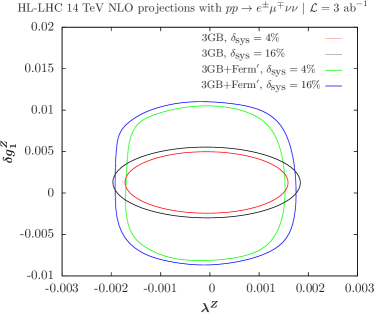
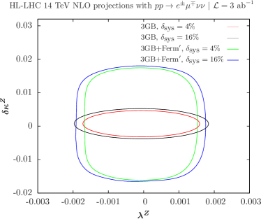
Figure 3: Same as in Fig. 1, but with the fermion couplings constrained to vary around 0. The curves allowing for $Z$-quark coupling to vary around 0 within the $2\sigma$ limit in Eq.(32) are labeled “3GB+Ferm^′”. The standard cuts given in Eqs. (26) and (27) are applied.

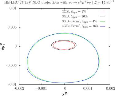
Figure 4: Same as in Fig. 2, but with the fermion couplings constrained to vary around 0. The curves allowing for $Z$-quark coupling to vary around 0 within the $2\sigma$ limit in Eq.(32) are labeled “3GB+Ferm^′”. The standard cuts given in Eqs. (26) and (27) are applied.

IV 13 TeV distributions

In this section, we demonstrate the use of the primitive cross sections to compute $K$-factors and distributions in the presence of anomalous couplings. The primitive cross sections at $13$ TeV (with and without the basic cuts of Eqs.(26) and (27)) are attached as supplemental material, including a variety of kinematic distributions of interest. The goal is to enable rapid scans over anomalous couplings at NLO QCD. Our scheme is similar to the reweighting used in MadGraph Mattelaer:2016gcx . We define a series of $K$-factors for the process $pp\rightarrow W^{+}W^{-}\rightarrow\mu^{\pm}e^{\mp}\nu{\overline{\nu}}$,

$$K_{SM} = {d\sigma_{SM}^{NLO}\over d\sigma_{SM}^{LO}},$$ (33)

$$K_{SMEFT}^{(n)} = {d\sigma_{SMEFT}^{NLO}(C_{1},C_{2}...C_{m})\over d\sigma_{SMEFT}^{LO}(C_{1},C_{2},...C_{m})},$$

$$S^{(n)}_{SMEFT} = {d\sigma_{SMEFT}^{NLO}(C_{1},C_{2}...C_{m})\over d\sigma_{SM}^{NLO}},$$ (34)

where $K_{SMEFT}^{(n)}$ and $S^{(n)}_{SMEFT}$ are evaluated in the SMEFT to ${\cal{O}}({\Lambda^{-2n}})$ and LO and NLO refer to the order in QCD. The notation $d\sigma$ can represent either differential or total cross sections, where the numerators and denominators must be evaluated with identical cuts. Applying the cuts of Eqs.(26) and (27), the SM total cross sections are,

$$\sigma^{LO}_{SM} = 0.383~{}pb,$$

$$\sigma^{NLO}_{SM} = 0.400~{}pb\,.$$ (35)

Figure 5: Primitive cross sections relevant at ${\cal{O}}(\Lambda^{-2})$, with $\vec{C}=(\delta g_{1}^{Z},\lambda^{A},\delta\kappa^{Z})$. $d\sigma(1,\vec{R}_{i})$ is defined by Eq.(10). The standard cuts given in Eqs. (26) and (27) are applied.

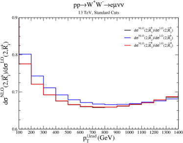
Figure 6: LHS: Primitive cross sections relevant at ${\cal{O}}(\Lambda^{-4})$, with $\vec{C}=(\delta g_{1}^{Z},\lambda^{A},\delta\kappa^{Z})$. RHS: Primitive cross sections relevant at ${\cal{O}}(\Lambda^{-4})$, normalized to the LO primitive cross sections. The black and red curves are almost indistinguishable. $d\sigma(2,\vec{R}_{i})$ is defined in by Eq.(10). The standard cuts given in Eqs. (26) and (27) are applied.

To ${\cal{O}}({\Lambda^{-2}})$, the SMEFT $K$-factor is,

$$K_{SMEFT}^{(1)} = K_{SM}\biggl{[}1-\Sigma_{i}C_{i}\biggl{(}r_{1i}^{LO}-r_{1i}^{NLO}\biggr{)}\biggr{]}\,,$$ (36)

where we have normalized,

$$r_{1i}^{LO} = {d\sigma^{LO}(1;\vec{R}_{i})\over d\sigma_{SM}^{LO}},$$

$$r_{1i}^{NLO} = {d\sigma^{NLO}(1;\vec{R}_{i})\over d\sigma_{SM}^{NLO}}\,,$$ (37)

where $d\sigma^{LO}(1;\vec{R}_{i})$ and $d\sigma^{NLO}(1;\vec{R}_{i})$ are the primitive functions defined in Eq.(10) evaluated at LO and NLO QCD, respectively. The primitive cross sections at ${\cal{O}}({\Lambda^{-2}})$ that are relevant for the case where only the 3-gauge-boson couplings are anomalous are shown in Fig. 5 for the leading lepton transverse momentum, $p_{T}^{\ell,lead}$. To ${\cal{O}}({\Lambda^{-4}})$, the analytic form for the $K_{SMEFT}^{(2)}$ factor becomes rather complicated and we evaluate it numerically using Eq.(11). Fig. 6 shows some of the primitive cross sections relevant at ${\cal{O}}({\Lambda^{-4}})$. Note that the effects of the NLO corrections are not the same as those in the SM, although in both cases there is a strong dependence on $p_{T}^{\ell,lead}$.

A useful form for expressing the results is,

$${S}_{SMEFT}^{(2)} = (1-\Sigma_{i=1}^{m}C_{i})+\Sigma_{i}C_{i}\biggl{[}{d\sigma^{NLO}(1;{\vec{R}}_{i})\over d\sigma_{SM}^{NLO}}\biggr{]},$$

$${S}_{SMEFT}^{(4)} = (1-\Sigma_{i=1}^{m}C_{i})+\Sigma_{i}C_{i}\biggl{[}{d\sigma^{NLO}(1;{\vec{R}}_{i})\over d\sigma_{SM}^{NLO}}\biggr{]}+\Sigma_{i=1}^{m}C_{i}^{2}\biggl{[}{d\sigma^{NLO}(2;{\vec{R}}_{i})-d\sigma^{NLO}(1;{\vec{R}}_{i})\over d\sigma_{SM}^{NLO}}\biggr{]},$$ (38)

$$+\Sigma_{i>j=1}^{m}C_{i}C_{j}\biggl{[}{d\sigma^{NLO}(2;\vec{M}_{ij})-d\sigma^{NLO}(2;{\vec{R}}_{i})-d\sigma^{NLO}(2;{\vec{R}}_{j})\over d\sigma_{SM}^{NLO}}+1\biggr{]}\,,$$

where $d\sigma$ can be distributions or total cross sections. At $13$ TeV with the usual cuts, see Eqs. (26) and (27), the $S^{(4)}_{SMEFT}$ factor for the total cross section is,

$${S}_{SMEFT}^{(4)} = 1+\biggl{[}-0.6305C_{1}+0.04881~{}C_{2}+0.1767~{}C_{3}+4.541~{}C_{4}-0.3212~{}C_{5}$$ (39)

$$-4.723~{}C_{6}+0.1327~{}C_{7}\biggr{]}+19.66~{}C_{1}^{2}+21.93~{}C_{2}^{2}+21.80~{}C_{3}^{2}+32.97~{}C_{4}^{2}$$

$$+36.92~{}C_{5}^{2}+44.39~{}C_{6}^{2}+25.45~{}C_{7}^{2}+\Sigma_{i>j=1}^{m}C_{i}C_{j}\biggl{[}X_{ij}\biggr{]}\,.$$

where the values of $X_{ij}$ are given in Table 3 and we define the coefficients, ${\vec{C}}=(\delta g_{1}^{Z},\lambda^{Z},\delta\kappa^{Z},\delta g_{L}^{Zu},\delta g_{R}^{Zu},\delta g_{L}^{Zd},\delta g_{R}^{Zd})$. The largest sensitivity of $S_{SMEFT}^{(4)}$ is to the left-handed $Z$-quark couplings, as also observed in Ref. Grojean:2018dqj . Eq.(39) can be rescaled by the NLO SM total cross section, Eq.(35), to obtain numerical values to NLO order for arbitrary SMEFT coefficients. Note that the numerical coefficients of Eq.(39) depend on the cuts.

$X_{ij}$	2	3	4	5	6	7
$1$	2.211	-31.35	-14.67	32.20	36.82	-10.77
$2$		-4.963	-2.372	-0.1275	2.931	0.05577
$3$			-13.49	-48.49	-14.66	9.676
$4$				-0.02663	-15.00	-0.02611
$5$					-0.001471	-0.003671
$6$						$0.0003033$

Table 3: Coefficients defined in Eq.(39) with ${\vec{C}}=(\delta g_{1}^{Z},\lambda^{Z},\delta\kappa^{Z},\delta g_{L}^{Zu},\delta g_{R}^{Zu},\delta g_{L}^{Zd},\delta g_{R}^{Zd})$ . The standard cuts given in Eqs. (26) and (27) are applied.

For comparison, we present $S^{(4)}_{SMEFT}$ in the HISZ basis of Eq.(8) using the primitive cross sections discussed above. Using the results of the previous section, $C_{i}=\Sigma_{j}\alpha_{ij}C_{j}^{\prime}$, with,

$$C_{i}=\left(\begin{matrix}\delta g_{1}^{Z}\\ \delta\kappa_{Z}\\ \lambda_{Z}\end{matrix}\right),\qquad C_{i}^{\prime}=\left(\begin{matrix}{\hat{f_{W}}}=f_{W}\biggl{(}{M_{Z}^{2}\over\Lambda^{2}}\biggr{)}\\ {\hat{f_{B}}}=f_{B}\biggl{(}{M_{Z}^{2}\over\Lambda^{2}}\biggr{)}\\ {\hat{f}}_{WWW}=f_{WWW}\biggl{(}{M_{Z}^{2}\over\Lambda^{2}}\biggr{)}\end{matrix}\right),\qquad\alpha=\left(\begin{matrix}{1\over 2}&0&0\\ {c_{W}^{2}\over 2}&-{s_{W}^{2}\over 2}&0\\ 0&0&{3g^{2}c_{W}^{2}\over 4}\end{matrix}\right)\,,$$ (40)

and $C_{i}=C_{i}^{\prime},~{}i=4-7$. The $S^{(4)}_{SMEFT}$ factor in a transformed basis is,

$$S_{SMEFT}^{(4)} = (1-\Sigma_{i,k=1}^{m}C_{i}^{\prime}\alpha_{ki})+\Sigma_{i,k=1}^{m}C_{i}^{\prime}\alpha_{ki}\biggl{[}{d\sigma^{NLO}(1;{\vec{R}}_{k})\over d\sigma_{SM}^{NLO}}\biggr{]}$$ (41)

$$+\Sigma_{i=1}^{m}C_{i}^{\prime~{}2}\biggl{\{}\Sigma_{k=1}^{m}\alpha_{ki}^{2}\biggl{[}{d\sigma^{NLO}(2;\vec{R}_{k})-d\sigma^{NLO}(1;\vec{R}_{k})\over d\sigma_{SM}^{NLO}}\biggr{]}$$

$$+\Sigma_{l=1}^{m}\Sigma_{k=l+1}^{m}\alpha_{ki}\alpha_{li}\biggl{[}{d\sigma^{NLO}(2,\vec{M}_{kl})-d\sigma^{NLO}(2;{\vec{R}_{k}})-d\sigma^{NLO}(2;{\vec{R}_{l}})\over d\sigma_{SM}^{NLO}}+1\biggr{]}\biggr{\}}$$

$$+\Sigma_{j=1}^{m}\Sigma_{i=j+1}^{m}C_{i}^{\prime}C_{j}^{\prime}\biggl{\{}\Sigma_{k=1}^{m}2\alpha_{ki}\alpha_{kj}\biggl{[}{d\sigma^{NLO}(2;\vec{R}_{k})-d\sigma^{NLO}(1;\vec{R}_{k})\over d\sigma_{SM}^{NLO}}\biggr{]}$$

$$+\Sigma_{l=1}^{m}\Sigma_{k=l+1}^{m}\biggl{(}\alpha_{kj}\alpha_{li}+\alpha_{ki}\alpha_{lj}\biggr{)}$$

$$\cdot\biggl{[}{d\sigma^{NLO}(2;\vec{M}_{kl})-d\sigma^{NLO}(2;\vec{R}_{k})-d\sigma^{NLO}(2;\vec{R}_{l})\over d\sigma_{SM}^{NLO}}+1\biggr{]}\biggr{\}}\,.$$

For $i,j=4-7$, $\alpha_{ij}=\delta_{ij}$. The primitive cross sections $d\sigma^{NLO}(n,\vec{R}_{i})$ and $d\sigma^{NLO}(n,\vec{M}_{ij})$ are defined in Eqs. (10,12) and are evaluated in the original anomalous couplings basis.

For the total cross section in the HISZ basis applying our basic cuts in Eqs. (26) and (27) with ${\vec{C}^{\prime}}=({\hat{f_{W}}},{\hat{f_{B}}},{\hat{f}}_{WWW},\delta g_{L}^{Zu},\delta g_{R}^{Zu},\delta g_{L}^{Zd},\delta g_{R}^{Zd})$ and $\Lambda=1$ TeV,

$$S^{(4)}_{SMEFT,~{}HISZ} = 1+\biggl{[}-0.4059C_{1}^{\prime}-1.115C_{2}^{\prime}-0.7189C_{3}^{\prime}$$ (42)

$$+4.541C_{4}^{\prime}-0.3211C_{5}^{\prime}-4.723C_{6}^{\prime}+0.1327C_{7}^{\prime}\biggr{]}$$

$$+8.687C^{\prime~{}2}_{1}+.2639C^{\prime~{}2}_{2}+1.2C^{\prime~{}2}_{3}+32.97C^{\prime~{}2}_{4}$$

$$+36.92C^{\prime~{}2}_{5}+44.39C^{\prime~{}2}_{6}+25.45C^{\prime~{}2}_{7}+\Sigma_{i>j=1}^{m}C_{i}^{\prime}C_{j}^{\prime}\biggl{[}{\hat{X}}_{ij}\biggr{]}\,.$$

where the values of ${\hat{X}}_{ij}$ are given in Table 4.

$\hat{X}_{ij}$	2	3	4	5	6	7
$1$	-1.447	-3.917	-14.67	32.20	36.82	-10.77
$2$		1.178	-2.372	-0.1275	2.931	0.05577
$3$			-13.49	-48.49	-14.66	9.676
$4$				-0.02663	-15.00	-0.02611
$5$					-0.001471	-0.003671
$6$						$0.0003033$

Table 4: HISZ basis coefficients defined in Eq. (42) with ${\vec{C}^{\prime}}=({\hat{f}}_{W},{\hat{f}}_{B},{\hat{f}}_{WWW},\delta g_{L}^{Zu},\delta g_{R}^{Zu},\delta g_{L}^{Zd},\delta g_{R}^{Zd})$ and $\Lambda=1$ TeV. The standard cuts given in Eqs. (26) and (27) are applied.

The primitive cross sections can also be used to study distributions with arbitrary SMEFT coefficients and we show some sample results for the transverse momentum of the leading charged lepton, $p_{T}^{\ell,lead}$, and for the invariant mass distribution of the charged leptons, $m_{\ell\ell}$. In Fig. 7, we show the distribution of the leading lepton $p_{T}$ in a scenario with only anomalous 3-gauge-boson couplings (LHS) and with only anomalous $Z-$ quark couplings (RHS). The values of the coefficients were chosen to be allowed by experimental limits from $W^{+}W^{-}$ pair production Aad:2016wpd ; Khachatryan:2015sga and from fits to LEP data Schael:2013ita , and to give similar $p_{T}$ distributions. It is apparent that the anomalous 3-gauge-boson-only and anomalous-$Z-$fermion-only scenarios cannot be distinguished by studying the $p_{T}$ distributions alone and that the dominant effects come from the $\Lambda^{-4}$ contributions. The NLO effects decrease the rate at high $p_{T}$ for the anomalous 3-gauge-boson couplings and increase it for anomalous $Z-$ fermion couplings.

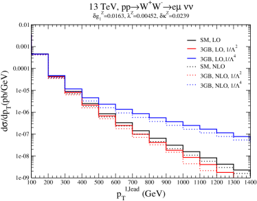
Figure 7: Distribution of the leading charged lepton $p_{T}$ in a scenario with only anomalous 3-gauge-boson couplings (LHS) and only anomalous $Z-$ fermion couplings (RHS) to ${\cal{O}}(\Lambda^{-2})$ and ${\cal{O}}(\Lambda^{-4})$ at LO and NLO QCD. The SM, LO and Ferm, LO, $1/\Lambda^{2}$ curves on the RHS are indistinguishable. The standard cuts given in Eqs. (26) and (27) are applied.

Figs. 8 and 9 we show the variables of Eq.(34). The $S^{(n)}_{SMEFT}$ variable compares the SMEFT distributions with those of the SM, demonstrating the dominance of the $\Lambda^{-4}$ terms at large $p_{T}$. SM and SMEFT $K$-factors are shown in Fig. 9 and it is clear that the SM and SMEFT scale similarly with small variations. Similarly, the K-factors for the anomalous-fermion-only scenario (RHS or Fig. 9) and the anomalous-3GB-only scenario (LHS of Fig. 9) are also similar with small variations. We note that this is for specific choices of the anomalous couplings and for different choices the $K$-factors have to be checked using the primitive cross sections.

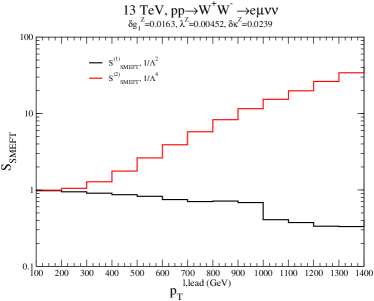
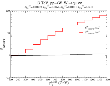
Figure 8: Comparison of the $S$ factors of Eq.(34) for the SM and SMEFT in the anomalous 3-gauge-boson-only scenario (LHS) and anomalous-fermion-only scenario (RHS) at ${\cal{O}}({\Lambda^{-2}})$ and ${\cal{O}}({\Lambda^{-4}})$ . The standard cuts given in Eqs. (26) and (27) are applied.

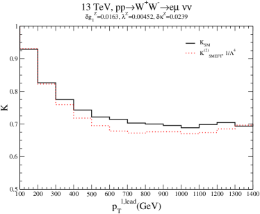
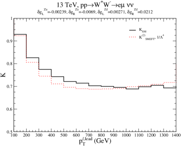
Figure 9: Comparison of the $K$-factors of Eq.(34) for the SM and SMEFT in the anomalous 3-gauge-boson-only scenario (LHS) and anomalous-fermion-only scenario (RHS). The standard cuts given in Eqs. (26) and (27) are applied.

In Fig. 10, we show the invariant mass distribution of the charged leptons in a scenario with only anomalous 3-gauge-boson couplings (LHS) and with only anomalous $Z-$ quark couplings (RHS). As is the case with the $p_{T}$ distributions, the dominant effect arises from the $\Lambda^{-4}$ contributions. Figs. 11 and 12 show the variables of Eq.(34). The $S^{(n)}_{SMEFT}$ variable compares the SMEFT distributions with those of the SM, again showing the large effects from the ${\cal{O}}(\Lambda^{-4})$ terms. SM and SMEFT $K$-factors are shown in Fig. 12 and are quite similar to each other.

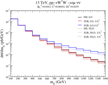
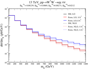
Figure 10: Invariant mass distribution in a scenario with only anomalous 3-gauge-boson couplings (LHS) and only anomalous fermion couplings (RHS) to ${\cal{O}}(\Lambda^{-2})$ and ${\cal{O}}(\Lambda^{-4})$ at LO and NLO QCD. The standard cuts given in Eqs. (26) and (27) are applied.

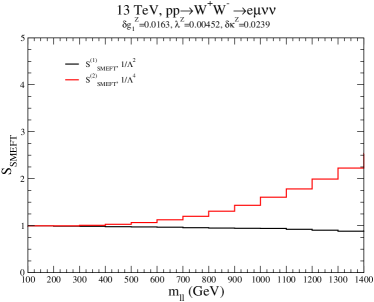
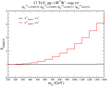
Figure 11: Comparison of the $S$ factors of Eq.(34) for the SM and SMEFT in the anomalous 3-gauge-boson-only scenario (LHS) and anomalous-fermion-only scenario (RHS). The standard cuts given in Eqs. (26) and (27) are applied.

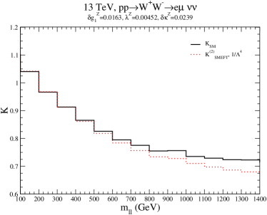
Figure 12: Comparison of the $K$-factors of Eq.(34) for the SM and SMEFT in the anomalous 3-gauge-boson-only scenario (LHS) and anomalous-fermion-only scenario (RHS). The standard cuts given in Eqs. (26) and (27) are applied.

Ref. Chiesa:2018lcs computes the NLO QCD (along with the NLO EW) corrections to gauge boson pair production when the fermion couplings take their SM values. Our results are qualitatively similar to theirs for the scenario with only anomalous 3-gauge-boson couplings.

V Conclusions

We have extended our previous NLO calculation of the contribution of anomalous couplings to $pp\rightarrow W^{+}W^{-}$ to include the leptonic decays, $pp\rightarrow W^{+}W^{-}\rightarrow\mu^{\pm}e^{\mp}\nu{\overline{\nu}}$ and implemented the results in the POWHEG-BOX. The primitive cross sections at $13$ TeV for a variety of observables are posted at https://quark.phy.bnl.gov/Digital_Data_Archive/dawson/ww_18. The most important implication of our results is the interplay between anomalous $Z$-quark couplings and anomalous 3-gauge-boson couplings requiring global fits to both fermion and gauge couplings in order to obtain reliable results. Our NLO results at $13$ TeV are presented in terms of primitive cross sections allowing for rapid scans over anomalous couplings in an arbitrary basis.

- (1) S. Dawson, C. Englert, and T. Plehn, “Higgs Physics: It ain’t over till it’s over,” arXiv:1808.01324 [hep-ph].
- (2) ATLAS, CMS Collaboration, G. Aad et al., “Measurements of the Higgs boson production and decay rates and constraints on its couplings from a combined ATLAS and CMS analysis of the LHC pp collision data at and 8 TeV,” JHEP 08 (2016) 045, arXiv:1606.02266 [hep-ex].
- (3) A. Butter, O. J. P. Eboli, J. Gonzalez-Fraile, M. C. Gonzalez-Garcia, T. Plehn, and M. Rauch, “The Gauge-Higgs Legacy of the LHC Run I,” JHEP 07 (2016) 152, arXiv:1604.03105 [hep-ph].
- (4) ATLAS Collaboration, M. Aaboud et al., “Measurement of the Higgs boson coupling properties in the decay channel at = 13 TeV with the ATLAS detector,” JHEP 03 (2018) 095, arXiv:1712.02304 [hep-ex].
- (5) ATLAS Collaboration, M. Aaboud et al., “Measurements of Higgs boson properties in the diphoton decay channel with 36 fb-1 of collision data at TeV with the ATLAS detector,” Phys. Rev. D98 (2018) 052005, arXiv:1802.04146 [hep-ex].
- (6) CMS Collaboration, A. M. Sirunyan et al., “Combined measurements of Higgs boson couplings in proton-proton collisions at 13 TeV,” arXiv:1809.10733 [hep-ex].
- (7) DELPHI, OPAL, LEP Electroweak, ALEPH, L3 Collaboration, S. Schael et al., “Electroweak Measurements in Electron-Positron Collisions at W-Boson-Pair Energies at LEP,” Phys. Rept. 532 (2013) 119–244, arXiv:1302.3415 [hep-ex].
- (8) M. J. Duncan, G. L. Kane, and W. W. Repko, “ Physics at Future Colliders,” Nucl. Phys. B272 (1986) 517–559.
- (9) K. Hagiwara, R. D. Peccei, D. Zeppenfeld, and K. Hikasa, “Probing the Weak Boson Sector in ,” Nucl. Phys. B282 (1987) 253–307.
- (10) Z. Zhang, “Time to Go Beyond Triple-Gauge-Boson-Coupling Interpretation of Pair Production,” Phys. Rev. Lett. 118 no. 1, (2017) 011803, arXiv:1610.01618 [hep-ph].
- (11) J. Baglio, S. Dawson, and I. M. Lewis, “An NLO QCD effective field theory analysis of production at the LHC including fermionic operators,” Phys. Rev. D96 no. 7, (2017) 073003, arXiv:1708.03332 [hep-ph].
- (12) A. Alves, N. Rosa-Agostinho, O. J. P. Eboli, and M. C. Gonzalez-Garcia, “Effect of Fermionic Operators on the Gauge Legacy of the LHC Run I,” Phys. Rev. D98 no. 1, (2018) 013006, arXiv:1805.11108 [hep-ph].
- (13) C. Grojean, M. Montull, and M. Riembau, “Diboson at the LHC vs LEP,” arXiv:1810.05149 [hep-ph].
- (14) W. Buchmuller and D. Wyler, “Effective Lagrangian Analysis of New Interactions and Flavor Conservation,” Nucl. Phys. B268 (1986) 621–653.
- (15) B. Grzadkowski, M. Iskrzynski, M. Misiak, and J. Rosiek, “Dimension-Six Terms in the Standard Model Lagrangian,” JHEP 10 (2010) 085, arXiv:1008.4884 [hep-ph].
- (16) J. Bellm, S. Gieseke, N. Greiner, G. Heinrich, S. Platzer, C. Reuschle, and J. F. von Soden-Fraunhofen, “Anomalous coupling, top-mass and parton-shower effects in production,” JHEP 05 (2016) 106, arXiv:1602.05141 [hep-ph].
- (17) T. Gehrmann, M. Grazzini, S. Kallweit, P. Maierhofer, A. von Manteuffel, S. Pozzorini, D. Rathlev, and L. Tancredi, “ Production at Hadron Colliders in Next to Next to Leading Order QCD,” Phys. Rev. Lett. 113 no. 21, (2014) 212001, arXiv:1408.5243 [hep-ph].
- (18) M. Grazzini, S. Kallweit, S. Pozzorini, D. Rathlev, and M. Wiesemann, “ production at the LHC: fiducial cross sections and distributions in NNLO QCD,” JHEP 08 (2016) 140, arXiv:1605.02716 [hep-ph].
- (19) S. Dawson, P. Jaiswal, Y. Li, H. Ramani, and M. Zeng, “Resummation of jet veto logarithms at N3LLa + NNLO for production at the LHC,” Phys. Rev. D94 no. 11, (2016) 114014, arXiv:1606.01034 [hep-ph].
- (20) K. Hamilton, T. Melia, P. F. Monni, E. Re, and G. Zanderighi, “Merging WW and WW+jet with MINLO,” JHEP 09 (2016) 057, arXiv:1606.07062 [hep-ph].
- (21) A. Bierweiler, T. Kasprzik, and J. H. Kuhn, “Vector-boson pair production at the LHC to accuracy,” JHEP 12 (2013) 071, arXiv:1305.5402 [hep-ph].
- (22) J. Baglio, L. D. Ninh, and M. M. Weber, “Massive gauge boson pair production at the LHC: a next-to-leading order story,” Phys. Rev. D88 (2013) 113005, arXiv:1307.4331 [hep-ph]. [Erratum: Phys. Rev.D94,no.9,099902(2016)].
- (23) B. Biedermann, M. Billoni, A. Denner, S. Dittmaier, L. Hofer, B. Jaeger, and L. Salfelder, “Next-to-leading-order electroweak corrections to 4 leptons at the LHC,” JHEP 06 (2016) 065, arXiv:1605.03419 [hep-ph].
- (24) J. M. Campbell, R. K. Ellis, and C. Williams, “Vector boson pair production at the LHC,” JHEP 07 (2011) 018, arXiv:1105.0020 [hep-ph].
- (25) M. Chiesa, A. Denner, and J.-N. Lang, “Anomalous triple-gauge-boson interactions in vector-boson pair production with RECOLA2,” Eur. Phys. J. C78 no. 6, (2018) 467, arXiv:1804.01477 [hep-ph].
- (26) L. J. Dixon, Z. Kunszt, and A. Signer, “Helicity amplitudes for O(alpha-s) production of , , , , or pairs at hadron colliders,” Nucl. Phys. B531 (1998) 3–23, arXiv:hep-ph/9803250 [hep-ph].
- (27) L. J. Dixon, Z. Kunszt, and A. Signer, “Vector boson pair production in hadronic collisions at order : Lepton correlations and anomalous couplings,” Phys. Rev. D60 (1999) 114037, arXiv:hep-ph/9907305 [hep-ph].
- (28) T. Melia, P. Nason, R. Rontsch, and G. Zanderighi, “W+W-, WZ and ZZ production in the POWHEG BOX,” JHEP 11 (2011) 078, arXiv:1107.5051 [hep-ph].
- (29) P. Nason and G. Zanderighi, “ , and production in the POWHEG-BOX-V2,” Eur. Phys. J. C74 no. 1, (2014) 2702, arXiv:1311.1365 [hep-ph].
- (30) A. Biekötter, D. Gonçalves, T. Plehn, M. Takeuchi, and D. Zerwas, “The Global Higgs Picture at 27 TeV,” arXiv:1811.08401 [hep-ph].
- (31) K. J. F. Gaemers and G. J. Gounaris, “Polarization Amplitudes for and ,” Z. Phys. C1 (1979) 259.
- (32) A. Azatov, R. Contino, C. S. Machado, and F. Riva, “Helicity selection rules and noninterference for BSM amplitudes,” Phys. Rev. D95 no. 6, (2017) 065014, arXiv:1607.05236 [hep-ph].
- (33) A. Falkowski, M. Gonzalez-Alonso, A. Greljo, D. Marzocca, and M. Son, “Anomalous Triple Gauge Couplings in the Effective Field Theory Approach at the LHC,” JHEP 02 (2017) 115, arXiv:1609.06312 [hep-ph].
- (34) A. Dedes, W. Materkowska, M. Paraskevas, J. Rosiek, and K. Suxho, “Feynman Rules for the Standard Model Effective Field Theory in -gauges,” arXiv:1704.03888 [hep-ph].
- (35) P. Nason, “A New method for combining NLO QCD with shower Monte Carlo algorithms,” JHEP 11 (2004) 040, arXiv:hep-ph/0409146 [hep-ph].
- (36) S. Frixione, P. Nason, and C. Oleari, “Matching NLO QCD computations with Parton Shower simulations: the POWHEG method,” JHEP 11 (2007) 070, arXiv:0709.2092 [hep-ph].
- (37) S. Alioli, P. Nason, C. Oleari, and E. Re, “A general framework for implementing NLO calculations in shower Monte Carlo programs: the POWHEG BOX,” JHEP 06 (2010) 043, arXiv:1002.2581 [hep-ph].
- (38) J. M. Campbell and R. K. Ellis, “An Update on vector boson pair production at hadron colliders,” Phys. Rev. D60 (1999) 113006, arXiv:hep-ph/9905386 [hep-ph].
- (39) ATLAS Collaboration, G. Aad et al., “Measurement of total and differential production cross sections in proton-proton collisions at 8 TeV with the ATLAS detector and limits on anomalous triple-gauge-boson couplings,” JHEP 09 (2016) 029, arXiv:1603.01702 [hep-ex].
- (40) C. Schmidt, J. Pumplin, D. Stump, and C. P. Yuan, “CT14QED parton distribution functions from isolated photon production in deep inelastic scattering,” Phys. Rev. D93 no. 11, (2016) 114015, arXiv:1509.02905 [hep-ph].
- (41) D. Liu and L.-T. Wang, “Precision Measurement with Diboson at the LHC,” arXiv:1804.08688 [hep-ph].
- (42) A. Falkowski and F. Riva, “Model-independent precision constraints on dimension-6 operators,” JHEP 02 (2015) 039, arXiv:1411.0669 [hep-ph].
- (43) A. Falkowski, M. Gonzalez-Alonso, and K. Mimouni, “Compilation of low-energy constraints on 4-fermion operators in the SMEFT,” JHEP 08 (2017) 123, arXiv:1706.03783 [hep-ph].
- (44) L. Berthier, M. Bjorn, and M. Trott, “Incorporating doubly resonant data in a global fit of SMEFT parameters to lift flat directions,” JHEP 09 (2016) 157, arXiv:1606.06693 [hep-ph].
- (45) O. Mattelaer, “On the maximal use of Monte Carlo samples: re-weighting events at NLO accuracy,” Eur. Phys. J. C76 no. 12, (2016) 674, arXiv:1607.00763 [hep-ph].
- (46) CMS Collaboration, V. Khachatryan et al., “Measurement of the cross section in pp collisions at 8 TeV and limits on anomalous gauge couplings,” Eur. Phys. J. C76 no. 7, (2016) 401, arXiv:1507.03268 [hep-ex].