Abstract: Earth observation satellites (EOSs) are specially designed to collect images according to user requirements. Agile EOSs (AEOSs), with stronger attitude maneuverability, greatly improve the observation capability, while increasing the complexity of scheduling the observations. We are the first to address multiple AEOSs scheduling with multiple observations where the objective function aims to maximize the entire observation profit over a fixed horizon. The profit attained by multiple observations for each target is nonlinear in the number of observations. Our model is a specific interval scheduling problem, with each satellite orbit represented as a machine. A column-generation-based framework is developed for this problem, in which the pricing problems are solved using a label-setting algorithm. Extensive computational experimtents are conducted on the basis of one of China’s AEOS constellations. The results indicate that our optimality gap is less than $3\%$ on average, which validates our framework. We also evaluate the performance of the framework for conventional EOS scheduling.

Keywords: agile Earth observation satellites, multiple observations, column generation heuristic, interval scheduling.

History: Submitted September 2018.

1 Introduction

Earth observation satellites (EOSs) with specialized cameras are designed to gather images according to user requirements. Broad applications of EOSs can be seen in the fields of Earth resource exploration, environmental monitoring and disaster surveillance, since EOSs provide a large-scale observation coverage. Due to the continuous decrease in launch cost and the improvement in small satellite technology, we are witnessing an explosive growth of the number of orbiting EOSs and planned launches, which can be expected to continue in the years to come (Nag et al.,, 2014). The scheduling of the EOSs is of great importance for the effective and efficient execution of observation missions.

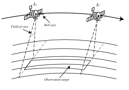
Figure 1: Illustration of the fixed observation interval of a conventional EOS.

Conventional EOS (CEOS) scheduling has been well studied (Lin et al.,, 2005; Vasquez and Hao,, 2001; Wolfe and Sorensen,, 2000) and agile EOS (AEOS) scheduling has also attracted significant attention in recent years (Lemaître et al.,, 2002). In CEOS scheduling, the EOS operates in its determined orbit and only has attitude adjustment ability along the roll axis. As can be seen in Figure 1, the CEOS can only observe the target during the visible time window ($VTW$) $[t_{a},t_{b}]$. The length of the $VTW$ is determined by the satellite and the observation target. Compared with a CEOS, an AEOS has stronger attitude adjustment capability, as it is maneuverable also on the pitch axis (Lemaître et al.,, 2002). Consequently, it may be possible for an AEOS to execute two or more observation missions within a single $VTW$, as long as all constraints are satisfied. In this article, we discretize each $VTW$ into multiple observation time windows ($OTW$s) with specific observation starting and ending times (we refer to Gabrel et al., (1997) and Wang et al., 2016b for further motivation of this choice). In other words, multiple candidate observation missions are generated for each $VTW$, each with fixed $OTW$.

As shown in the left part of Figure 2, a CEOS has a specific $OTW$ $[t_{a},t_{b}]$, which is the same as its $VTW$. There is no difference between the $VTW$ and $OTW$ for the CEOS, while the $VTW$ for an AEOS is longer than the corresponding $OTW$ because of the satellite’s ability to look ahead and look back. In the right part of Figure 2, the AEOS can start an observation mission for the target at $t_{c}$, or begin observation at $t_{e}$ later than $t_{a}$. In this way, CEOS scheduling is a $VTW$ selection problem (Lemaître et al.,, 2002), while each $VTW$ contains multiple potential $OTW$s for an AEOS. Although agile satellites greatly improve the observation capability, the complexity of observation scheduling in comparison with CEOS scheduling also increases dramatically.

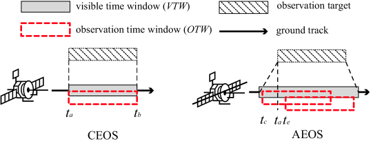
Figure 2: Comparison of the observation capability for CEOS and AEOS.

We divide the scheduling horizon into several satellite orbits, which correspond with the circles of the satellite around the Earth (see Gabrel and Vanderpooten, (2002) and Wang et al., 2016a for similar choices). During one satellite orbit, the satellite passes the same target only once, thus each $VTW$ corresponds to one specific satellite orbit.

Multiple observations for the same target can help to achieve stereo and/or time-series observations (Gorney et al.,, 1986; Nichol et al.,, 2006; Stearns and Hamilton,, 2007). It is desirable for each target to be observed more than once, and the target observation profit relates nonlinearly to the observation count. To the best of our knowledge, however, none of the existing models in this domain can be readily applied to handle multiple observations: previous models only allow for one observation mission within one $VTW$. In this paper, we address a scheduling problem with multiple AEOSs and multiple observations, which will be referred to as MAS. Problem MAS can be regarded as a specific interval scheduling problem in a parallel machine environment, with each orbit of each satellite represented as a machine. Various practical constraints, including mission transformation, memory and energy consumption are included. A large number of $OTW$s (potential mission intervals) are generated for each target during the $VTW$ discretization procedure, making it difficult to apply existing interval scheduling algorithms for solving MAS.

The main contributions of this paper are threefold: (1) to the best of our knowledge, scheduling multiple AEOSs with multiple observations has not been studied before; we define the problem MAS with a nonlinear profit function. (2) Since MAS cannot be effectively handled by a general commercial solver in a straightforward manner, we propose a column-generation-based framework based on a reformulation of a compact linear formulation. (3) We also test the proposed framework for CEOS scheduling and report our findings.

The remainder of this paper is structured as follows. In Section 2 we provide an extensive literature review. A problem statement and formulation are presented in Section 3. The column generation (CG) framework is sketched in Section 4. Section 5 contains a series of computational results which demonstrate the performance of the proposed framework. We conclude the work in Section 6.

2 Literature review

2.1 EOSs scheduling

In this subsection, we provide a survey of recent work on the related subjects of CEOS and AEOS scheduling.

Gabrel and Vanderpooten, (2002) formulate a CEOS scheduling problem as the selection of a path optimizing multiple criteria in a graph without circuit. Based on the EOS SPOT 5 (ESA,, 2002), Vasquez and Hao, (2001) present a formulation as a generalized version of the well-known knapsack model, which includes large numbers of logical constraints. Constraint satisfaction procedures have also been introduced for CEOS scheduling with a set of hard constraints (Bensana et al.,, 1996; Sun et al.,, 2008). Lin et al., (2005) study the daily imaging CEOS scheduling for the EOS ROCSAT-II (ESA,, 2004), and develop an integer programming (IP) model with different imaging rewards. For the case where potentially hundreds of orbiting satellites are used to execute observation missions, a window-constrained packing model for CEOS scheduling is established by Wolfe and Sorensen, (2000), and their work also considers an extended model with multiple resources and multiple observation opportunities for the same target. Wang et al., (2015); Wang et al., 2016a further extend the foregoing models by consideration of uncertainty of cloud coverage and real-time scheduling.

Optimal solutions for CEOS scheduling problems can be found for small instances. Gabrel and Vanderpooten, (2002) solve CEOS scheduling problems with a single satellite using a graph-theoretical procedure. Bensana et al., (1996) propose a depth-first branch-and-bound (B&B) algorithm with constraint satisfaction ingredients, requiring limited space. Upper bounds for CEOS scheduling problems have been studied in Benoist and Beno, (2004) and Vasquez and Hao, (2003). Since exact methods may fail to find optimal solutions in reasonable runtimes, approximate algorithms are viable practical alternatives for CEOS scheduling, especially for large instances with multiple satellites. Various versions of genetic algorithms have been developed for CEOS scheduling (Wolfe and Sorensen,, 2000; Baek et al.,, 2011; Kim and Chang,, 2015; Kolici et al.,, 2013), and local search techniques have also been widely applied (Vasquez and Hao,, 2001; Lemaître et al.,, 2002; Kolici et al.,, 2013). Other heuristic methods have also been studied; Wolfe and Sorensen, (2000), for instance, propose a constructive method with fast and simple priority dispatch. Lin et al., (2005) describe a Lagrangian relaxation heuristic to obtain near-optimal solutions. Wang et al., (2011) develop a decision support system considering mission conflicts.

The complexity of agile satellite scheduling is significantly higher than for the conventional case. Gabrel et al., (1997) first studied single AEOS scheduling using graph-theoretical concepts. Various classes of approximate methods have been developed for AEOS scheduling since Lemaître et al., (2002) explicitly introduced this problem in the early 21$st$ century; the authors design four simple heuristic algorithms. Considering stereoscopic and visibility constraints, Habet et al., (2010) formulate AEOS scheduling as a constrained optimization problem and propose a tabu search method with partial enumeration. Tangpattanakul et al., (2015) adopt a local search heuristic for AEOS scheduling, and compare with a biased random-key genetic algorithm. Wang et al., 2016b model AEOS scheduling by means of a directed acyclic graph, regarding each node as a discrete observation mission, and propose a heuristic to scan the graph. Liu et al., (2017) construct an adaptive large neighborhood search metaheuristic with six removal operators and three insertion operators.

The studies mentioned in the previous paragraph all relate to single AEOSs, while only limited attention has been paid so far to jointly scheduling multiple agile satellites. Considering the integrated scheduling of two AEOSs and transmission operations, Globus et al., (2003) test the performance of several search techniques including simulated annealing, random swap mutations and priority ordering. Li et al., (2007) present a combined genetic algorithm for multiple AEOS scheduling, where the fitness computation for their genetic algorithm is conducted by simulated annealing. Xu et al., (2016) define priority-based indicators and employ a sequential construction procedure to generate feasible solutions. It is worth noting that the previous models do not allow for more than one observation mission within one $VTW$, and multiple observations for the same target have, as far as we are aware, not yet been studied for AEOS scheduling. Incorporating multiple observations for multiple agile satellites and producing solutions with performance guarantee on the optimality gap are still unexplored subjects in the literature; these are exactly the topics that are studied in this article.

2.2 Interval scheduling

In interval scheduling, the processing times of the jobs and their starting times are both given, and it needs to be decided whether or not to accept each job and which resource to assign to it. Comprehensive surveys of interval scheduling are presented in Kolen et al., (2007) and Kovalyov et al., (2007). Fischetti et al., (1987, 1989, 1992) study the so-called “fixed job scheduling” problem with specific practical timing constraints, and propose several polynomial-time approximate algorithms. Kroon et al., (1995) characterize the “fixed interval scheduling” problem and develop exact and approximation algorithms. The proposed algorithms have been applied in practical settings such as satellite communication systems (Bar-Noy et al.,, 2012), semiconductor manufacturing (Cakici and Mason,, 2007), and waterway infrastructure (Gedik et al.,, 2016).

3 Definitions and problem statement

In Section 3.1, we present the basic model MAS, with multiple observations and multiple agile satellites. We will assume that each satellite can only observe one target at a given time, and that observation preemption is not allowed. Subsequently, in Section 3.2, we extend the basic formulation with practical constraints regarding mission transformation, energy consumption and memory capacity.

3.1 MAS

Denote $T$ as the set of targets and $\omega_{i}$ as the profit for target $i\in T$. In line with the definitions of observation profits of Lemaître et al., (2002) and Cordeau and Laporte, (2005), we assume that the marginal benefit of an extra observation increases with the number of observations for each target $i$, up until a maximum desired observation number $N_{i}$ within the time horizon (although this property is not essential to the model). The observation profit $\omega_{i}$ for target $i$ is a nonlinear function of the observation count, which can be written in linearized form as $\omega_{i}=\sum_{s=0}^{s=N_{i}}\pi_{is}y_{is}$ with $\sum_{s=0}^{s=N_{i}}y_{is}=1$, where all $y_{is}$ are binary variables ($i\in T$, $s=0,\ldots,N_{i}$). When $s$ observations are scheduled for target $i$ then $\pi_{is}$ is the observation profit (a nonnegative integer) and $y_{is}=1$; otherwise $y_{is}=0$. We let $y_{iN_{i}}=1$ when the number of missions for target $i$ is greater than $N_{i}$, since no additional profit would be received.

An illustration of the profit function of a target $i$ is provided in Figure 3, with the maximum number of missions $N_{i}=4$, and $\pi_{i0}=0$, $\pi_{i1}=1$, $\pi_{i2}=3$, $\pi_{i3}=6$ and $\pi_{i4}=10$.

Figure 3: Illustration of the profit function.

Define $S$ as the set of satellites, and let $B_{j}$ represent the set of orbits for satellite $j\in~{}S$. The set of candidate observation missions in orbit $k\in B_{j}$ is defined as $M_{jk}$. Each candidate observation mission $p\in M_{jk}$ is expressed as a pair $(OTW_{jkp},i)$, indicating that each observation mission is associated with a corresponding target $i$ and a specific $OTW$.

We will consider sequence-dependent constraints concerning mission transformation and energy in Section 3.2. To ensure that these constraints can be easily incorporated into the model, the binary decision variable $x_{jkpq}$ is adopted with $x_{jkpq}=1$ when observation mission $q$ is the immediate successor of $p$ in orbit $k\in B_{j}$; $x_{jkpq}=0$ otherwise. For each satellite orbit, we add dummy missions $s_{jk}$ and $e_{jk}$ as source and sink node, respectively. The number of observations scheduled for target $i$ is then expressed as $\sum\limits_{j\in{S}}\sum\limits_{k\in{B_{j}}}\sum\limits_{p\in{M_{jk}^{i}}}\sum\limits_{q\in{M_{jk}\cup{\{e_{jk}\}}}}x_{jkpq}$, where $M_{jk}^{i}$ stands for the observation mission set associated with target $i$ in orbit $k\in B_{j}$. A compact linear formulation of MAS can then be stated as follows:

max $$\sum\limits_{i\in{T}}\sum_{s=1}^{s=N_{i}}\pi_{is}y_{is}$$ (1)

subject to $$\sum\limits_{q\in{M_{jk\cup e}}}x_{jkpq}-\sum\limits_{q\in{M_{jk\cup s}}}x_{jkqp}=\begin{cases}1,&p=s_{jk}\\ 0,&\forall{p\in{M_{jk}}}\\ -1,&p=e_{jk}\end{cases} \forall k\in{B_{j}},j\in{S}$$ (2)

$$\sum\limits_{j\in{S}}\sum\limits_{k\in{B_{j}}}\sum\limits_{{p\in{M_{jk}^{i}}}}\sum\limits_{q\in{M_{jk\cup e}}}x_{jkpq}\geq\sum_{s=0}^{s=N_{i}}s\cdot y_{is} \forall{i}\in{T}$$ (3)

$$\sum_{s=0}^{s=N_{i}}y_{is}=1 \forall{i}\in{T}$$ (4)

where $M_{jk\cup s}=M_{jk}\cup\{s_{jk}\}$ and $M_{jk\cup e}=M_{jk}\cup\{e_{jk}\}$.

The objective function (1) aims to maximize the observation profit for the targets. The constraints (2) represent flow generation and conservation constraints. Constraints set (3) guarantees that the profits are computed correctly according to the number of scheduled observations, and constraints (4) ensure that each target receives exactly one profit value.

3.2 Extensions

The transformation time $\Delta_{jkpq}^{T}$ between two observation missions $p$ and $q$ in orbit $k\in B_{j}$ consists of attitude maneuvering time $\Delta_{jkpq}^{V}$ and attitude stabilization time $\Delta_{jkpq}^{S}$, which are given as inputs (Wertz,, 1978). Since the orbital duration of an AEOS is much larger than the transformation time between missions, the transformation constraint for two observation missions in different orbits is always satisfied, and is not imposed separately. This allows to partition each satellite’s time horizon into independent orbits, which greatly reduces the number of constraints. The transformation constraints are checked in a preprocessing stage: decision variable $x_{jkpq}$ is defined only if the sum of the completion time of mission $p$ and $\Delta_{jkpq}^{T}$ is not greater than the starting time of mission $q$ in orbit $k\in B_{j}$.

The memory capacity in one orbit of satellite $j$ is defined as $M^{C}_{j}$, and the unit-time imaging memory occupation is denoted as $M^{I}_{j}$. The memory capacity constraints are formulated per orbit, since we assume that satellites can transfer data to the ground station after each orbit. The energy system of an AEOS is typically partially supported by a solar panel collecting energy from the Sun. Although the conditions for solar energy collection are variable due to environmental variation, the amount of energy collection in one orbit is nearly constant (Wang et al., 2016a, ). We therefore assume that the maximal energy capacity of satellite $j$ is constant and denoted as $E^{C}_{j}$ in each orbit. Unit-time imaging energy consumption and maneuvering energy consumption are defined as $E^{I}_{j}$ and $E^{M}_{j}$ for satellite $j$, respectively. The number of observation missions in each orbit is limited to satisfy memory and energy constraints.

The extended formulation for MAS is then to maximize (1) subject to (2)–(4) and

$$\sum\limits_{{p\in{M_{jk}}}}\sum\limits_{q\in{M_{jk\cup e}}}x_{jkpq}d_{jkp}M^{I}_{j}\leq{M^{C}_{j}} \forall{k}\in{B_{j}},{j}\in{S}$$ (5)

$$\sum\limits_{{p\in{M_{jk}}}}\sum\limits_{q\in{M_{jk\cup e}}}x_{jkpq}d_{jkp}E^{I}_{j}+\sum\limits_{{p\in{M_{jk}}}}\sum\limits_{{q\in{M_{jk}}}}x_{jkpq}\Delta_{jkpq}^{V}E^{M}_{j}\leq{E^{C}_{j}} \forall{k}\in{B_{j}},{j}\in{S}$$ (6)

where $d_{jkp}$ is the observation duration of $OTW_{jkp}$. Clearly, these knapsack-type constraints imply that the problem is NP-hard.

4 Column generation

CG is a promising method to tackle formulations with a huge number of variables (Barnhart et al.,, 1998; Wilhelm,, 2001; Lübbecke and Desrosiers,, 2005; Gschwind et al.,, 2018). This technique has been used for decades since CG was first applied to the cutting stock problem as part of an efficient heuristic algorithm (Gilmore and Gomory,, 1961, 1963). The main advantage of CG is that not all variables need to be explicitly included into the model. In this section, we decompose the linear relaxation of the compact formulation of Section 3, leading to a CG-based solution framework for the LP-relaxation. We design a column initialization heuristic, and iteratively solve a restricted master problem (RMP) with restricted column set by a commercial LP-solver. We apply a label-setting method to find solutions to the pricing problems in the GC-procedure, thus iteratively adding new columns until the optimal solution of the RMP is found. The integrality constraints are then re-imposed using all the generated columns to obtain a high-quality solution with an IP-solver. In light of the large number of variables for MAS in practice, in the corresponding B&B routine we do not generate new columns for the new LP-problems encountered upon branching because this would become overly time-consuming. In other words, we apply a CG-heuristic and we do not implement a branch-and-price procedure. Similar choices are frequently made in the literature, for instance in Furini et al., (2012) and Guedes and Borenstein, (2015). We will show in Section 5 that the tight LP-bound confirms that a near-optimal integer solution is usually obtained in this way.

4.1 Dantzig-Wolfe decomposition

The flow-based formulation of Section 3 has been used to design heuristic and constructive algorithms (Lin et al.,, 2005; Liu et al.,, 2017), but it is difficult to evaluate the optimality gap for such procedures. Exact methods, on the other hand, fail to obtain optimal solutions for large instances (Gabrel and Vanderpooten,, 2002). Since the constraints are decoupled into different orbits, we apply Dantzig-Wolfe reformulation (Martin,, 2012) to decompose the original model.

The schedules in each satellite orbit are regarded as columns. Denote the set of schedules in satellite orbit $k\in B_{j}$ as $R_{jk}$. Each schedule $m\in R_{jk}$ contains values $x_{jkpq}^{m}$, where $x_{jkpq}^{m}=1$ if mission $p$ is the immediate predecessor of mission $q$ according to schedule $m$ in orbit $k\in S_{j}$; $x_{jkpq}^{m}=0$ otherwise. We introduce a binary variable $z_{jkm}$ for each $m\in R_{jk}$ such that $z_{jkm}=1$ when schedule $m$ is chosen and 0 otherwise. The master problem then aims to maximize (1) subject to (4) and

$$\sum\limits_{j\in{S}}\sum\limits_{k\in{B_{j}}}\sum\limits_{m\in{R_{jk}}}\sum\limits_{{p\in{M_{jk}^{i}}}}\sum\limits_{q\in{M_{jk\cup e}}}x_{jkpq}^{m}z_{jkm}\geq\sum_{s=1}^{s=N_{i}}s\cdot y_{is} \forall{i}\in{T}$$ (7)

$$\sum\limits_{m\in{R_{jk}}}z_{jkm}=1 \forall k\in{B_{j}},{j}\in{S}$$ (8)

where constraints (7) correspond with (3) in the original flow formulation and constraints (8) ensure that only one orbit schedule is selected for each satellite orbit. For each orbit, new columns are iteratively generated according to the results of the pricing problems detailed in Section 4.2.

4.2 The pricing problems

We remove the integrality constraints to obtain the LP relaxation of the master problem. With dual variables ${\theta}_{i}^{1}$ associated with constraints (7), variables ${\theta}_{i}^{2}$ with constraints (4), and variables ${\theta}_{jk}^{3}$ with constraints (8), we have the following dual:

min $$\sum\limits_{i\in{T}}{\theta}^{2}_{i}+\sum\limits_{j\in{S}}\sum\limits_{k\in{B_{j}}}{\theta}^{3}_{jk}$$ (9)

s.t. $$-s{\theta}^{1}_{i}+{\theta}^{2}_{i}\geq\pi_{is} \forall{s}\in\{1,2,\ldots,N_{i}\},{i}\in{T}$$ (10)

$$\sum\limits_{i\in{T}}{\theta}^{1}_{i}\sum\limits_{{p\in{M_{jk}^{i}}}}\sum\limits_{q\in{M_{jk\cup e}}}x_{jkpq}^{m}+{\theta}^{3}_{jk}\geq 0 \forall m\in{R_{jk}},k\in{B_{j}},{j}\in{S}$$ (11)

$${\theta}^{1}_{i}\leq 0,{\theta}^{2}_{i}\in\mathbb{R} \forall{{i}\in{T}}$$ (12)

$${\theta}^{3}_{jk}\in\mathbb{R} \forall k\in{B_{j}},{j}\in{S}$$ (13)

At each CG-iteration we check the violation of constraints (11). The LP relaxation is typically solved faster if we add constraints that are strongly violated, and we will search for columns with most negative reduced cost. Considering the special structure of the dual formulation, we end up with a separate pricing problem for each satellite orbit $k\in B_{j}$, as follows:

min $$\sum\limits_{i\in{T}}{\theta}^{1}_{i}\sum\limits_{p\in{M_{jk}^{i}}}\sum\limits_{q\in{M_{jk\cup e}}}x_{jkpq}+{\theta}^{3}_{jk}$$ (14)

s.t. $$\sum\limits_{q\in{M_{jk\cup e}}}x_{jkpq}-\sum\limits_{q\in{M_{jk\cup s}}}x_{jkqp}=\begin{cases}1,&p=s_{jk}\\ 0,&\forall{p\in{M_{jk}}}\\ -1,&p=e_{jk}\end{cases}$$ (15)

$$\sum\limits_{{p\in{M_{jk}}}}\sum\limits_{q\in{M_{jk\cup e}}}x_{jkpq}d_{jkp}M^{I}_{j}\leq{M^{C}_{j}}$$ (16)

$$\sum\limits_{{p\in{M_{jk}}}}\sum\limits_{q\in{M_{jk\cup e}}}x_{jkpq}d_{jkp}E^{I}_{j}+\sum\limits_{{p\in{M_{jk}}}}\sum\limits_{{q\in{M_{jk}}}}x_{jkpq}\Delta_{jkpq}^{V}E^{M}_{j}\leq{E^{C}_{j}}$$ (17)

For each pricing problem, if the optimal value is less than 0 then a new column for the corresponding orbit is generated with lowest reduced cost; otherwise no new column results. The CG-iterations continue until all pricing problems return an optimal value not less than 0, demonstrating that there are no violated constraints (11). The corresponding LP objective value constitutes a tight upper bound for problem MAP.

4.3 Column initialization

Our column initialization heuristic proceeds as follows. For each satellite orbit, the algorithm attempts to generate initial columns for given number iterations. In each iteration, the observation missions are re-ordered randomly and it is checked whether they can be greedily added into the current schedule. Since different orbit schedules may have different contributions to the overall profit, we introduce the following definition.

Definition 1.

Column dominance. For a satellite orbit, column dominance occurs when the number of scheduled observations for any target in one (dominant) column is no less than the observation number of the corresponding target in another (dominated) column, and for at least one target, the observation number of the dominant column is strictly greater than in the dominated column.

Property 1.

If one column is dominated by the existing columns, it can be discarded without deteriorating the objective function.

The dominated column can be discarded since the dominant column that has higher contribution to objective. A generated column is discarded if it is dominated; otherwise it is added to the initial column pool. Similarly, if a column currently in the column pool is dominated by a new column then it is also removed.

4.4 Label-setting method for pricing

The pricing problem for each satellite orbit corresponds to a resource-constrained shortest path problem (Pugliese and Guerriero,, 2013) in a graph without circuit. We use an adaptation of a label-setting algorithm (Gabrel and Vanderpooten,, 2002) to solve this problem. For each satellite orbit $k\in B_{j}$, we define a directed acyclic graph $G_{jk}=(N_{jk},E_{jk})$, where the vertex set $N_{jk}$ contains all candidate observation missions and dummy missions $s_{jk}$ and $e_{jk}$. The edge set $E_{jk}$ contains an edge from mission (node) $p$ to mission (node) $q$ only if $q$ can be executed immediately after $p$; we also include an edge from $s_{jk}$ to each other vertex, and $e_{jk}$ has edges incoming from all other vertices.

Definition 2.

Mission path. In the directed acyclic graph $G_{jk}=(N_{jk},E_{jk})$, a mission path is a path from the dummy source to any observation mission or the dummy sink mission $q\in N_{jk}\setminus\{s_{jk}\}$. A mission path can be represented as a tuple $P_{jkqt}=(Cost_{jkqt},CurM_{jkqt},CurE_{jkqt})$, where $Cost_{jkqt}$ is the sum of the mission costs along the path, $CurM_{jkqt}$ and $CurE_{jkqt}$ are the summed memory occupation and energy consumption, respectively, and value $t$ is an index for the mission paths ending at mission $q$ in $G_{jk}$.

For each observation mission $q$ in graph $G_{jk}$, the mission cost $MisCost_{jkq}$ equals $\theta^{1}_{i}$, where $i$ is the target associated with mission $q$ (see objective function (14)). The mission memory occupation and energy consumption are denoted as $MisM_{jkq}$ and $MisE_{jkq}$. For the dummy source and sink missions, the mission cost is set as $\theta^{3}_{jk}/2$, and the mission memory and energy consumption are set to 0. Searching a column with the most negative reduced cost in orbit $k\in B_{j}$ now transforms to searching a constrained path with minimal mission cost from source to sink in $G_{jk}$. The resource constraints ensure that the total memory occupation and energy consumption along each path do not exceed the corresponding capacity.

Denote the set of mission paths ending at mission $q$ in $G_{jk}$ as $\mathscr{P}_{jkq}$. Property 2 below enhances algorithmic efficiency of the label-setting method used to find a minimal-cost path; the details of the method are described in Appendix A.

Definition 3.

Mission path dominance. In the set $\mathscr{P}_{jkq}$ for a given mission $q$ in $G_{jk}$, mission path $P_{jkq{t_{1}}}$ dominates $P_{jkq{t_{2}}}$ when the following inequalities hold and at least one of the inequalities is strict: 1) $Cost_{jkqt_{1}}\leq Cost_{jkqt_{2}}$; 2) $CurM_{jkqt_{1}}\leq CurM_{jkqt_{2}}$; 3) $CurE_{jkqt_{1}}\leq CurE_{jkqt_{2}}$.

Property 2.

For the pricing problem in a given satellite orbit, a dominated mission path can be discarded without loss of optimality.

Proof.

Without loss of generality, we denote the dominant and dominated path as $P_{jkq{t_{1}}}$ and $P_{jkq{t_{2}}}$ in $\mathscr{P}_{jkq}$, respectively. Assume that there exists a shortest path $P_{jke_{jk}t}$ in $G_{jk}$ including path $P_{jkq{t_{2}}}$. If we replace $P_{jkq{t_{2}}}$ by $P_{jkq{t_{1}}}$ while maintaining the subsequent path from $q$ to $e_{jk}$, we obtain a new feasible path $P_{jke_{jk}t^{\prime}}$ satisfying all resource constraints and with $Cost_{jke_{jk}t^{\prime}}\leq Cost_{jke_{jk}t}$. ∎

5 Computational experiments

5.1 Data generation

Since there is no common benchmark for AEOS scheduling (Liu et al.,, 2017), the proposed CG-based framework is tested on a diverse set of realistic instances that is generated as follows. Our satellite configuration is based on China’s high-resolution AEOSs Gaojing-1 (also known as SuperView-1) (SpaceView,, 2018). Gaojing-1 is a commercial constellation of four remote sensing satellites. Details of the satellites’ parameters are provided in Appendix B.

Following Liu et al., (2017), the observation targets are randomly distributed worldwide, and in specific interest areas. We consider these two target distributions together in the same instance within 24 hours, with 150 globally distributed targets and several specific interest areas with 50 targets. The number of interest areas varies from 0 to 3. Therefore the total number of observation targets is 150, 200, 250 or 300. The desired maximum observation number $N_{i}$ for each target $i$ is randomly generated from 1 to 5 and the maximal profit $\pi_{iN_{i}}$ for each target is defined as an integer number from 1 to 10. Since the satellites in the Gaojing-1 constellation have very similar properties, the constraints for each satellite are taken to be identical. The unit-time imaging memory occupation $M^{I}$ is 10 MB per second, while the unit-time imaging consumption $E^{I}$ and maneuvering energy consumption $E^{M}$ are 500 and 1000 Watt, respectively. The memory capacity $M^{C}$ is set as 400, 500 or 600 MB. The energy capacity $E^{C}$ is considered in electric charge from 30, 40, 50 or 60 kilojoules (kJ). The discretization unit of each $VTW$ is set as two seconds (see Section 5.2.4 for more information). With the above settings, the length of each $VTW$ is around 90 seconds, generating about 45 $OTW$s. For each combination of parameter settings, 10 instances are randomly generated.

5.2 Computational results

5.2.1 Experimental setup

The computational experiments are conducted on a laptop equipped with Intel Core i5-7200 CPU at 2.5 GHz and 8 GB of RAM on a Windows 10 64-bit OS. The algorithm is implemented in Visual C++. The LP- and IP-solver is CPLEX 12.6.3 using Concert Technology with four threads on two cores. The time limit for each run is set as 1200 seconds. In the tables below, the columns labelled $opt$ and $time$ contain the number of instances solved to guaranteed optimality out of 10 instances per setting and the average CPU time for the 10 instances in seconds, respectively. Columns $ub$ show the number of instances for which the LP is successfully solved to optimality, providing the upper bound. The entries labelled $gap$ represent the relative gap between the scheduling solution and the LP-bound obtained from the CG-based framework.

5.2.2 Results for AEOS instances

We first look into the results of the compact flow formulation by CPLEX in Table 1. Clearly, The flow formulation struggles already with with the smallest instances, especially when the memory capacity increases. For the instances with 150 globally distributed targets, only 24 out of 120 instances are solved to optimality, and its overall runtime is orders of magnitude higher than for the CG-based framework reported below. Due to this poor computational performance, we will not further include this formulation for comparison on larger instances.

Table 1: Results of the flow formulation on instances with 150 targets.

$M^{C}$	$E^{C}$	$opt$ $(/10)$	$time$
400	30	0	1200.00
	40	0	1200.00
	50	9	566.09
	60	10	255.93
500	30	0	1200.00
	40	0	1200.00
	50	0	1200.00
	60	5	797.94
600	30	0	1200.00
	40	0	1200.00
	50	0	1200.00
	60	0	1200.00
Overall		24	1035.00

Next, we report results for the CG-based framework. We denote our algorithm with label-setting pricing solver as CG-LAB, and we compare with CG-CPL in in which we call CPLEX to solve the pricing problems. The outcomes are summarized in Tables 2 to 5, for instances with number of targets ranging from 150 to 300.

Table 2: Computational results of CG-LAB and CG-CPL on instances with 150 targets.

		CG-CPL			CG-LAB
$M^{C}$	$E^{C}$	$ub$ $(/10)$	$time$		$ub$ $(/10)$	$time$		$gap$
400	30	10	760.24		10	36.70		2.56
	40	6	966.23		10	37.20		1.60
	50	10	129.14		10	20.21		0.84
	60	10	151.98		10	11.29		0.90
500	30	10	864.85		10	36.70		2.56
	40	3	1155.61		10	37.20		1.60
	50	2	1183.87		10	20.21		0.84
	60	10	206.12		10	11.29		0.90
600	30	10	631.21		10	36.70		2.56
	40	3	1179.33		10	37.20		1.60
	50	0	1200.00		10	20.21		0.84
	60	0	1200.00		10	11.29		0.90
Overall		74	802.38		120	26.35		1.48

Table 3: Computational results of CG-LAB and CG-CPL on instances with 200 targets.

		CG-CPL			CG-LAB
$M^{C}$	$E^{C}$	$ub$ $(/10)$	$time$		$ub$ $(/10)$	$time$		$gap$
400	30	2	1187.84		10	78.75		3.23
	40	0	1200.00		10	81.95		2.26
	50	10	206.48		10	43.03		0.98
	60	10	182.45		10	26.32		0.92
500	30	0	1200.00		10	74.92		3.17
	40	0	1200.00		10	93.60		2.64
	50	0	1200.00		10	109.18		2.40
	60	10	232.87		10	75.69		1.81
600	30	0	1200.00		10	74.43		3.23
	40	0	1200.00		10	95.02		2.59
	50	0	1200.00		10	118.69		2.62
	60	0	1200.00		10	140.14		2.63
Overall		32	950.80		120	84.31		2.37

Table 4: Computational results of CG-LAB and CG-CPL on instances with 250 targets.

		CG-CPL			CG-LAB
$M^{C}$	$E^{C}$	$ub$ $(/10)$	$time$		$ub$ $(/10)$	$time$		$gap$
400	30	0	1200.00		10	167.03		4.47
	40	0	1200.00		10	242.30		3.53
	50	7	814.75		10	187.30		2.47
	60	7	735.94		10	172.99		2.19
500	30	0	1200.00		10	174.39		4.38
	40	0	1200.00		10	341.53		3.49
	50	0	1200.00		10	457.51		3.94
	60	7	866.69		10	396.45		3.71
600	30	0	1200.00		10	176.77		4.36
	40	0	1200.00		10	333.33		3.46
	50	0	1200.00		10	467.29		3.34
	60	0	1200.00		10	537.73		4.10
Overall		21	1101.45		120	304.55		3.62

Table 5: Computational results of CG-LAB and CG-CPL on instances with 300 targets.

		CG-CPL			CG-LAB
$M^{C}$	$E^{C}$	$ub$ $(/10)$	$time$		$ub$ $(/10)$	$time$		$gap$
400	30	0	1200.00		10	224.15		4.08
	40	0	1200.00		10	313.74		3.47
	50	3	999.46		10	255.57		2.96
	60	3	980.87		10	249.29		2.53
500	30	0	1200.00		10	219.12		4.52
	40	0	1200.00		10	417.71		3.76
	50	0	1200.00		10	601.15		4.57
	60	2	1070.50		10	494.25		4.29
600	30	0	1200.00		10	199.31		4.35
	40	0	1200.00		10	351.59		3.61
	50	0	1200.00		9	700.49		3.90
	60	0	1200.00		9	862.59		4.78
Overall		8	1154.24		118	407.41		3.90

Overall, CG-LAB consistently outperforms CG-CPL, obtaining the upper bound for all instances from 150 to 250 targets and only failing for two instances with 300 targets. CG-CPL, on the other hand, already starts to experience difficulties on the smallest instances with 150 targets. As the number of targets increases, the performance of CG-CPL becomes worse, in that the LP is usually not solved within the time limit. With 300 targets, CG-CPL can only solve eight out of 120 instances. The cause of CG-CPL’s failure is the time required for the pricing problems. Although the label-setting pricing solver typically finds a shortest path very efficiently, CG-LAB fails to provide the upper bound on two instances with 300 targets; in these instances the number of mission paths for the pricing problem is close to one million, and the label-setting procedure also runs into difficulties. After the CG-procedure, the integer master problem with all generated columns is easily solved in less than one second in all cases.

As for the quality of the scheduling solutions, the average relative gap of CG-LAB is less than $3\%$. As the number of targets increases, the gap from the upper bound rises slightly but never exceeds $5\%$ for any instance. It is worth pointing out that the actual optimality gap for the solution produced by CG-LAB is typically smaller than the $gap$ value, while an optimal solution cannot be obtained in limited time.

The memory capacity $M^{C}$ significantly influences algorithmic performance. Larger $M^{C}$ provides more possibilities to execute more observation missions, while it also requires more time to solve the pricing problem for both of the algorithms. For CG-LAB, longer running times are required as $M^{C}$ increases, but the upper bound is still obtained for most instances, while CG-CPL gets stuck in the pricing problem due to the runtime limitations.

Different energy capacity values $E^{C}$ have different impact on the computational performance. For smaller $E^{C}$, the number of selected observation missions is low and fewer paths are generated, so a shorter running time is therefore needed for solving the pricing problem. When $E^{C}$ increases, on the other hand, a decrease in running time is sometimes also observed when larger $E^{C}$ no longer restrains the number of observation missions, so that the relaxed energy constraint is never binding anymore and thus does not have much impact anymore on the runtime.

5.2.3 Results for CEOS instances

The CG-based framework is developed for scheduling agile satellites, so it can also be applied for planning conventional satellites. By fixing a satellite along the pitch axis, we transform an AEOS into a CEOS. The same target distribution and orbital parameters of the satellite constellation are considered. We compare CG-LAB, CG-CPL and the compact flow formulation FF; the results are represented in Tables 6 to 9. The columns opt-gap report the gap between the solution of CG-LAB and the optimal integer solution obtained by FF, which is always readily available. On the instances with 150, 200 and 250 targets, FF needs less than one second on average for producing an optimal solution. CG-LAB always outperforms CG-CPL because of the pricing solver, and the size of the instance does not have a strong impact on its running time. Even for the largest instance with 300 targets, CG-LAB only requires 3.35 seconds on average, while over 60 seconds are needed for FF.

The solutions produced by the CG-heuristic are near-optimal. Compared with the LP-bound, the gap is less than $1\%$ on average and never exceeds $3\%$ for any instance. For these conventional instances, we can also compute the actual optimality gap opt-gap, which is even more favorable. For the instances with 150 and 200 targets, CG-LAB always finds an optimal solution. For the larger instances, the optimality gap is less than $0.1\%$. Overall, FF can efficiently find an optimal solution for small CEOS instances, while CG-LAB obtains produces near-optimal solutions for larger instances with less runtime than FF.

Table 6: Computational results for CEOS instances with 150 targets.

		CG-LAB	CG-CPL	FF
$M^{C}$	$E^{C}$	$time$	$time$	$time$	$gap$	opt-gap
400	30	2.25	9.50	0.10	0.62	0.00
	40	2.30	8.69	0.09	0.39	0.00
	50	2.34	8.31	0.06	0.25	0.00
	60	2.39	7.65	0.05	0.16	0.00
500	30	2.31	9.49	0.09	0.62	0.00
	40	2.36	9.05	0.10	0.41	0.00
	50	2.39	8.70	0.07	0.28	0.00
	60	2.37	7.65	0.05	0.16	0.00
600	30	2.39	9.18	0.09	0.62	0.00
	40	2.35	8.52	0.10	0.41	0.00
	50	2.47	9.02	0.07	0.27	0.00
	60	2.45	8.05	0.05	0.16	0.00
Overall		2.36	8.65	0.08	0.36	0.00

Table 7: Computational results for CEOS instances with 200 targets.

		CG-LAB	CG-CPL	FF
$M^{C}$	$E^{C}$	$time$	$time$	$time$	$gap$	opt-gap
400	30	2.79	12.78	0.60	1.21	0.00
	40	2.75	11.78	0.46	0.69	0.00
	50	2.80	10.60	0.21	0.44	0.00
	60	2.76	10.23	0.11	0.37	0.00
500	30	2.72	12.71	0.59	1.21	0.00
	40	2.87	12.31	0.48	0.69	0.00
	50	2.96	11.14	0.29	0.44	0.00
	60	2.90	10.78	0.20	0.33	0.00
600	30	2.71	11.61	0.59	1.21	0.00
	40	0.69	11.45	0.53	2.80	0.00
	50	0.46	11.54	0.38	2.97	0.00
	60	0.34	11.15	0.26	2.98	0.00
Overall		2.23	11.51	0.39	1.28	0.00

Table 8: Computational results for CEOS instances with 250 targets.

		CG-LAB	CG-CPL	FF
$M^{C}$	$E^{C}$	$time$	$time$	$time$	$gap$	opt-gap
400	30	2.53	11.92	0.75	1.25	0.00
	40	2.60	12.00	0.38	0.80	0.00
	50	2.57	10.97	0.17	0.47	0.01
	60	2.65	10.49	0.11	0.44	0.01
500	30	2.60	12.94	0.55	1.27	0.00
	40	2.78	12.97	0.45	0.83	0.00
	50	2.72	12.51	0.19	0.54	0.00
	60	2.80	10.97	0.14	0.36	0.01
600	30	2.62	12.72	0.69	1.27	0.01
	40	2.74	15.62	0.49	0.84	0.00
	50	2.75	12.02	0.23	0.57	0.00
	60	2.84	11.60	0.15	0.39	0.00
Overall		2.68	12.23	0.36	0.72	0.00

Table 9: Computational results for CEOS instances with 300 targets.

		CG-LAB	CG-CPL	FF
$M^{C}$	$E^{C}$	$time$	$time$	$time$	$gap$	opt-gap
400	30	3.16	15.03	106.88	1.52	0.05
	40	3.31	13.94	8.99	0.93	0.11
	50	3.15	12.50	1.67	0.54	0.08
	60	3.21	12.37	0.61	0.45	0.08
500	30	3.20	14.80	123.11	1.57	0.03
	40	3.35	14.93	122.09	1.14	0.05
	50	3.35	13.87	9.94	0.63	0.11
	60	3.44	13.85	1.73	0.43	0.10
600	30	3.16	13.88	123.48	1.64	0.11
	40	3.44	16.39	122.16	1.18	0.07
	50	3.66	16.08	100.54	0.77	0.08
	60	3.73	14.89	36.04	0.52	0.07
Overall		3.35	14.38	63.10	0.84	0.08

5.2.4 Sensitivity analysis

The discretization unit (the time between the start of two successive $OTW$s) of the $VTW$s is a key parameter of the model. In this section, we examine its influence on the performance of the proposed CG-based framework. We generate ten AEOS instances of 200 targets, combining 150 globally distributed targets and 50 targets in one interest area. The memory and energy capacity are fixed as 500 MB and 50 kJ, respectively. The simulation results for different discretization units are reported in Table 10, where column $dt$ represents the discretization unit in seconds and $|M|$ stands for the number of generated candidate observation missions. The columns $gap$ and $time$ contain the average value per setting only for the instances with an optimal LP-solution.

Table 10: Performance of CG-LAB with different discretization units.

$dt$	$|M|$	$ub$ $(/10)$	$gap$	$time$
1	22999	7	2.09	314.89
1.5	16695	10	2.28	203.09
2	12980	10	2.51	117.27
5	5242	10	2.25	30.66
10	2682	10	2.31	13.96
15	1828	10	1.48	9.15
20	1396	10	1.96	7.94

The number of generated missions clearly rises as $dt$ decreases. When $dt=1$ second, we cannot obtain the LP-bound for three out of the 10 instances because of an excessive number of missions. The gap from the LP-bound, on the other hand, is not very sensitive to $dt$, and is always below $3\%$. The value of $dt$ does have a very serious impact on the CPU time, with lower choices for $dt$ obviously leading to longer runtimes. The FF model cannot find an optimal solution within time limit even when $dt=20$ seconds. In conclusion, the user should carefully select a proper value of $dt$ for the proposed model, in order to strike a balance between fine discretization and running time.

6 Conclusions

In this article, we have studied the scheduling of observations by multiple agile satellites and with the possibility of conducting multiple observations for the same target. We aim to maximize the entire observation profit, with a profit function per target that can be nonlinear in the number of scheduled missions. We describe a linear flow-based formulation, which can handle sequence-dependent constraints but whose computational performance turns out to be limited.

We also develop a CG-based framework to solve a decomposition of the flow formulation. A label-setting algorithm is introduced for solving the pricing problems. We compare the flow model and two CG-heuristics, in which the pricing problem is solved by a label-setting algorithm and by an IP-solver, respectively. The computational results indicate that the flow formulation efficiently obtains optimal solutions on small instances for conventional satellite scheduling, while the CG-heuristic has superior performance for scheduling agile satellites, and the dedicated pricing solver is clearly better than the IP-solver for pricing. The proposed CG-framework also provides a tight upper bound that allows to effectively evaluate the quality of heuristic solutions.

Future research for agile satellite planning can be oriented in several directions. The objective function can be adjusted to incorporate completion times for the user-required missions, since rapid response plays a very important role in many observation missions, for instance in case of natural disasters. A more accurate modelling of data transmission constraints is also an avenue for future research. Finally, another planning complexity that has recently received some research attention but which deserves to be further explored, is related to the anticipation of uncertainty, for instance regarding cloud coverage.

Appendix A The label-setting procedure

Following Gabrel and Vanderpooten, (2002), we apply a label-setting method for the pricing problems. Since each edge in each graph $G_{jk}$ leads to a mission with a strictly larger starting time than its origin node, we order the missions $M_{jk}$ in ascending observation starting time so that all paths are explored by the loop between lines 1 and 14 in Algorithm 1.

For each mission $q$ in $G_{jk}$, we denote the set of possible predecessors as $M^{-q}_{jk}$ and employ function $GetCurPreMisIndex()$ to obtain the mission index of the current predecessor. Each path associated with mission $r$ in $\mathscr{P}_{jkr}$ is extended by adding the current $MisCost_{jkq}$, $MisM_{jkq}$ and $MisE_{jkq}$. Function $CheckConstraints()$ returns $true$ when $NewP$ satisfies all constraints and returns $false$ otherwise. Function $CheckPathDominance()$ returns $true$ if $NewP$ is not dominated by any paths in $\mathscr{P}_{jkq}$ and returns $false$ otherwise. Subsequently, $NewP$ can be added into $\mathscr{P}_{jkq}$ if $NewP$ is not dominated. We also check whether $NewP$ dominates any paths in $\mathscr{P}_{jkq}$, which can then be removed. Eventually, we obtain a path from source to sink with minimal cost.

The wrost-case complexity of Algorithm 1 is exponential, where $n$ is the number of vertices in the graph and exponential runtimes are unavoidable, knowing that the resource-constrained shortest path problem is NP-hard even with one resource (Mehlhorn and Ziegelmann,, 2000). In practice, however, the number of dominant paths may be relatively low thanks to the resource constraints and dominance criteria (Gabrel and Vanderpooten,, 2002), and the foregoing procedure empirically turns out to be a computationally viable alternative.

Procedure 1 The label-setting procedure

0:  candidate observation missions set $M_{jk}$ ordered in ascending observation starting time, possible predecessor set $M^{-q}_{jk}$ for each mission and other associated parameters;

0:  minimum of objective function (14);

1:  for each mission $q\in M_{jk}\cup\{e_{jk}\}$ do

2:     $P_{jkq}=\emptyset;$  

3:     for each possible predecessor mission in $M^{-q}_{jk}$ do

4:        $r=GetCurPreMisIndex();$ 

5:        for each $P_{jkrt^{\prime}}\in\mathscr{P}_{jkr}$  do

6:           $NewP=(Cost_{jkrt^{\prime}}+MisCost_{jkq},CurM_{jkrt^{\prime}}+MisM_{jkq},CurE_{jkrt^{\prime}}+MisE_{jkq})$; 

7:           if  $CheckConstraints(NewP)$ then

8:              if  $CheckPathDominance(\mathscr{P}_{jkq},NewP)$ then

9:                 $\mathscr{P}_{jkq}=\mathscr{P}_{jkq}\cup\{NewP\};$ 

10:              end if

11:           end if

12:        end for

13:     end for

14:  end for

15:  return  a minimal-cost path in $\mathscr{P}_{jke_{jk}}$

Appendix B Satellite parameters

Table 11 contains the following details for the four satellites in Gaojing-1. The first column ID indicates the name of satellite, and the parameters in the remaining columns are the satellite’s semi-major axis $a$, inclination $i$, right ascension of the ascending node $\Omega$, eccentricity $e$, argument of perigee $\omega$ and mean anomaly $M$, respectively. In addition, the agile platform of the constellation allows up to $30^{\circ}$ maneuvers along both the roll and the pitch axis.

Table 11: Orbital parameters of the satellite constellation Gaojing-1.

ID	$a$ (km)	$i$ (∘)	$\Omega$ (∘)	$e$	$\omega$ (∘)	$M$ (∘)
$Sat1$	6903.673	97.5839	97.8446	0.0016546	50.5083	2.0288
$Sat2$	6903.730	97.5310	95.1761	0.0015583	52.2620	31.4501
$Sat3$	6909.065	97.5840	93.1999	0.0009966	254.4613	155.2256
$Sat4$	6898.602	97.5825	92.3563	0.0014595	276.7332	140.1878

References

- Baek et al., (2011) Baek, S.-W., Han, S.-M., Cho, K.-R., Lee, D.-W., Yang, J.-S., Bainum, P. M., and Kim, H.-D. (2011). Development of a scheduling algorithm and GUI for autonomous satellite missions. Acta Astronautica, 68(7-8):1396–1402.
- Bar-Noy et al., (2012) Bar-Noy, A., Ladner, R. E., Tamir, T., and VanDeGrift, T. (2012). Windows scheduling of arbitrary-length jobs on multiple machines. Journal of Scheduling, 15(2):141–155.
- Barnhart et al., (1998) Barnhart, C., Johnson, E. L., Nemhauser, G. L., Savelsbergh, M. W. P., and Vance, P. H. (1998). Branch-and-price: Column generation for solving huge integer programs. Operations Research, 46(3):316–329.
- Benoist and Beno, (2004) Benoist, T. and Beno, R. (2004). Upper bounds for revenue maximization in a satellite scheduling problem. 4OR - Quarterly Journal of the Belgian, French and Italian Operations Research Societies, 2(3):235–249.
- Bensana et al., (1996) Bensana, E., Verfaillie, G., Agnese, J., Bataille, N., and Blumstein, D. (1996). Exact and inexact methods for the daily management of an earth observation satellite. In Proceeding of the international symposium on space mission operations and ground data systems, volume 4, pages 507–514.
- Cakici and Mason, (2007) Cakici, E. and Mason, S. J. (2007). Parallel machine scheduling subject to auxiliary resource constraints. Production Planning and Control, 18(3):217–225.
- Cordeau and Laporte, (2005) Cordeau, J.-F. and Laporte, G. (2005). Maximizing the value of an earth observation satellite orbit. Journal of the Operational Research Society, 56(8):962–968.
- ESA, (2002) ESA (2002). Spot-5. Available at {https://earth.esa.int/web/guest/missions/3rd-party-missions/current-missions/spot-5}.
- ESA, (2004) ESA (2004). Formosat-2 / ROCSat-2. Available at {https://directory.eoportal.org/web/eoportal/satellite-missions/content/-/article/formosat-2#spacecraft}.
- Fischetti et al., (1987) Fischetti, M., Martello, S., and Toth, P. (1987). The fixed job schedule problem with spread-time constraints. Operations Research, 35(6):849–858.
- Fischetti et al., (1989) Fischetti, M., Martello, S., and Toth, P. (1989). The fixed job schedule problem with working-time constraints. Operations Research, 37(3):395–403.
- Fischetti et al., (1992) Fischetti, M., Martello, S., and Toth, P. (1992). Approximation algorithms for fixed job schedule problems. Operations Research, 40(1-supplement-1):S96–S108.
- Furini et al., (2012) Furini, F., Malaguti, E., Durán, R. M., Persiani, A., and Toth, P. (2012). A column generation heuristic for the two-dimensional two-staged guillotine cutting stock problem with multiple stock size. European Journal of Operational Research, 218(1):251–260.
- Gabrel et al., (1997) Gabrel, V., Moulet, A., Murat, C., and Paschos, V. T. (1997). A new single model and derived algorithms for the satellite shot planning problem using graph theory concepts. Annals of Operations Research, 69:115–134.