A coarse-grid incremental pressure-projection method for accelerating low Reynolds-number incompressible flow simulations

Abstract

Coarse grid projection (CGP) multigrid techniques are applicable to sets of equations that include at least one decoupled linear elliptic equation. In CGP, the linear elliptic equation is solved on a coarsened grid compared to the other equations, leading to savings in computations time and complexity. One of the most important applications of CGP is when a pressure correction scheme is used to obtain a numerical solution to the Navier-Stokes equations. In that case there is an elliptic pressure Poisson equation. Depending on the pressure correction scheme used, the CGP method and its performance in terms of acceleration rate and accuracy level vary. The CGP framework has been established for non-incremental pressure projection techniques. In this article, we apply CGP methodology for the first time to incremental pressure correction schemes. Both standard and rotational forms of the incremental algorithms are considered. The influence of velocity Dirichlet and natural homogenous boundary conditions in regular and irregular domains with structured and unstructured triangular finite element meshes is investigated. $L^{2}$ norms demonstrate that the level of accuracy of the velocity and the pressure fields is preserved for up to three levels of coarsening. For the test cases investigated, the speedup factors range from 1.248 to 102.715.

1 Introduction and motivation

Projection methods [1–3] are popular schemes for simulating the unsteady incompressible Navier-Stokes equations, since the technique overcomes the saddle-point issue of the mass and momentum conservation equations by replacing those two equations with two decoupled elliptic ones: a nonlinear advection diffusion equation and a linear Poisson equation. Notwithstanding this benefit, the solution of Poisson’s equation is a major issue as it imposes high computational expenses to the system [4, 5].

Since we deal with the nonlinear convection term in the momentum equation, high spatial resolution is a key for conservation of the fidelity of the velocity field, especially for high Reynolds numbers. On the other hand, as the Poisson equation is a linear partial differential equation, such a refined grid resolution is not essential for its solution. Hence, an idea to accelerate these types of simulations is to solve the nonlinear momentum equation on a fine grid and compute the pressure Poisson equation on a corresponding coarsened grid. In 2010 Lentine et al. [4] first proposed this multiresolution technique, called Coarse Grid Projection (CGP) methodology, to lessen the computational cost associated with the Poisson equation for inviscid flow simulations. In 2013 San and Staples [5] expanded CGP to the incompressible Navier-Stoke equations (labeled “CGPRK3”). Moreover, they applied the CGP technique to elliptic equations of potential vorticity in quasigeostrophic ocean models [6]. In 2014 Jin and Chen [7] used CGP for the fast fluid dynamics (FFD) models to study building airflows. In 2018 Kashefi and Staples [8–11] presented a semi-implicit-time integration finite-element version of the CGP method (labeled “IFE-CGP”).

In all the methods cited above, the authors [4–6, 8–11] applied CGP to the non-incremental pressure projection scheme [1–3]. There are several limitations with this scheme which affect the efficiency of the CGP algorithm. The performance of the CGP technique can be measured by means of two technical parameters: speedup factor and accuracy level. For each CGP simulation, we look for how many levels of coarsening can be performed while preserving the accuracy level in either the velocity or the pressure field, and the associated computational speedup. The CGPRK3 approach [5] significantly reduced the integrity of the pressure field even for one coarsening level. In addition, a considerable reduction in the accuracy of the velocity field was observed for two and three levels of coarsening. San and Staples [5] achieved speedup factors ranging from roughly 2 to 42 using CGPRK3. Kashefi and Staples [9] demonstrated that IFECGP was only able to preserve the accuracy of the pressure gradient not the pressure itself (see e.g., Fig. 12 of Ref. [9]). Like CGPRK3, the IFE-CGP computations lost the superb fidelity of the velocity field for more than one coarsening level. The splitting error of the non-incremental pressure correction method [1–2] is irreducibly first-order in time with Dirichlet boundary conditions [3]. Due to the artificial Neumann boundary conditions for the pressure, the overall accuracy of this projection scheme is dominated by the temporal error rather than the spatial one [3]. Hence, IFE-CGP experienced shortcomings with realistic boundary conditions. The speedup factors of the numerical studies by IFE-CGP ranged from approximately 2 to 30.

To obviate the aforementioned problems, we implement the CGP strategy in the incremental pressure correction schemes including the standard [3, 12] and rotational [3, 12–13] forms. Taking this approach, the Poisson equation is solved on a coarsened grid for an intermediate variable and not for the pressure itself. Combining incremental pressure projection methods and CGP enhances the CGP capability in several ways. First, CGP preserves the accuracy of the velocity and the pressure field for a high level of the Poisson equation grid coarsening and thus remarkable speedup is reached. Second, since the incremental pressure projection scheme in standard form has an irreducible second-order time stepping error [3], a CGP algorithm with the standard form is improved from temporal integration point of view. Third, the incremental pressure correction technique in rotational form overcomes the artificial layers caused by the artificial homogenous pressure Neumann conditions [3]. Hence, a CGP method with the rotational form inherits this feature as well. We investigate the performance of the CGP algorithm in incremental pressure correction schemes through three standard test cases: the Taylor-Green vortex [14] with velocity Dirichlet boundary conditions in a square, the Jobelin vortex [12] with open boundary conditions in a square, and the Jobelin vortex [12] with velocity Dirichlet boundary conditions in a circle.

The present work is structured as follows. The governing equations for incompressible flows and their spatial/temporal discretizations are given in Sect. 2.1. The CGP algorithm and its computational consideration are discussed in Sect. 2.2 and Sect. 2.3, respectively. Numerical results are collected in Sect. 3 and conclusion is given in Sect. 4.

2 Problem formulation

2.1 Governing equations

We consider an incompressible isothermal flow of a Newtonian fluid, which is governed by the dimensionless form of the Navier-Stokes and continuity equations:

$$\bigg{[}\frac{\partial\textbf{{u}}}{\partial t}+(\textbf{{u}}\cdot\nabla)\textbf{{u}}\bigg{]}-\frac{1}{Re}\Delta\textbf{{u}}+\nabla p=\textbf{{f}}\textrm{ in }V,$$ (1)

$$\nabla\cdot\textbf{{u}}=0\textrm{ in }V,$$ (2)

$$\textbf{{u}}=\textbf{{u}}_{\Gamma_{D}}\textrm{ on }\Gamma_{D},$$ (3)

$$-p\textbf{{n}}+\frac{1}{Re}\nabla\textbf{{u}}\cdot\textbf{{n}}=\textbf{{t}}_{\Gamma_{N}}\textrm{ on }\Gamma_{N},$$ (4)

where u and $p$ stand for the velocity vector and the pressure of the fluid in domain $V$, respectively. f represents the vector of external force and $\textbf{{t}}_{\Gamma_{N}}$ denotes the stress vector. $Re$ is the Reynolds number. $\Gamma_{D}$ and $\Gamma_{N}$ respectively represent the Dirichlet and Neumann boundaries of the domain $V$, where n denotes the outward unit vector normal to them. Note that there is no overlapping between $\Gamma_{D}$ and $\Gamma_{N}$ subdomains.

Discretizing the system of equations using a second order backward differentiation formula [15] with respect to the time variable yields to:

$$\bigg{[}\frac{\frac{3}{2}\textbf{{u}}^{n+1}-2\textbf{{u}}^{n}+\frac{1}{2}\textbf{{u}}^{n-1}}{\delta t}+((2\textbf{{u}}^{n}-\textbf{{u}}^{n-1})\cdot\nabla)\textbf{{u}}^{n+1}\bigg{]}$$ (5)

$$-\frac{1}{Re}\Delta\textbf{{u}}^{n+1}+\nabla p^{n+1}=\textbf{{f}}^{n+1}\textrm{ in }V,$$

$$\nabla\cdot\textbf{{u}}^{n+1}=0\textrm{ in }V,$$ (6)

$$\textbf{{u}}^{n+1}=\textbf{{u}}_{\Gamma_{D}}^{n+1}\textrm{ on }\Gamma_{D},$$ (7)

$$-p^{n+1}\textbf{{n}}+\frac{1}{Re}\nabla\textbf{{u}}^{n+1}\cdot\textbf{{n}}=\textbf{{t}}_{\Gamma_{N}}^{n+1}\textrm{ on }\Gamma_{N},$$ (8)

where $\delta t$ represents the time step. In order to obtain the numerical solution of Eqs. (5)–(8), we utilize incremental pressure correction schemes [3]. Accordingly, at each time step $t^{n+1}$, we solve two cascading elliptic problems: a linearized equation for the intermediate velocity field $\tilde{\textbf{{u}}}^{n+1}$, and a linear Poisson’s equation for an intermediate variable $\phi$. Afterwards, the end-of-step velocity $\textbf{{u}}^{n+1}$ and the pressure $p^{n+1}$ are calculated through two correction equations. The corresponding equations are as follows:

$$\bigg{[}\frac{\frac{3}{2}\textbf{{\~{u}}}^{n+1}-2\textbf{{u}}^{n}+\frac{1}{2}\textbf{{u}}^{n-1}}{\delta t}+((2\textbf{{u}}^{n}-\textbf{{u}}^{n-1})\cdot\nabla)\textbf{{\~{u}}}^{n+1}\bigg{]}$$ (9)

$$-\frac{1}{Re}\Delta\textbf{{\~{u}}}^{n+1}=-\nabla p^{n}+\textbf{{f}}^{n+1}\textrm{ in }V,$$

$$\textbf{{\~{u}}}^{n+1}=\textbf{{u}}_{\Gamma_{D}}^{n+1}\textrm{ on }\Gamma_{D},$$ (10)

$$-p\textbf{{n}}+\frac{1}{Re}\nabla\textbf{{\~{u}}}^{n+1}\cdot\textbf{{n}}=\textbf{{t}}_{\Gamma_{N}}^{n+1}\textrm{ on }\Gamma_{N},$$ (11)

$$\Delta\phi=\frac{3}{2}\frac{1}{\delta t}\nabla\cdot\textbf{{\~{u}}}^{n+1}\textrm{ in }V,$$ (12)

$$\nabla\phi\cdot\textbf{n}=0\textrm{ on }\Gamma_{D},$$ (13)

$$\phi=0\textrm{ on }\Gamma_{N},$$ (14)

$$\textbf{{u}}^{n+1}=\textbf{{\~{u}}}^{n+1}-\frac{2}{3}\delta t\nabla\phi,$$ (15)

$$p^{n+1}=p^{n}+\phi-\chi\frac{1}{Re}\nabla\cdot\textbf{{\~{u}}}^{n+1},$$ (16)

where $\chi$ is a coefficient. If $\chi=0$ the standard form of the incremental pressure correction scheme is captured, whereas $\chi=1$ leads to the rotational form of the method.

Eqs. (9)–(16) can be spatially discretized using any desired method. Here, we use the finite element Galerkin scheme [13] to approximate the space of velocity and pressure. Since the projection method overcomes the saddle-point issue of Eqs. (1)–(2), satisfying the discrete Brezzi-Babuska condition [17, 18] is not essential [13]. Hence, the piecewise linear basis function (P₁/P₁) is implemented for the discretization of both the velocity and pressure variables. With this in mind, the finite element form of Eqs. (9)–(16) is expressed as

$$\frac{1}{\delta t}\big{(}\frac{3}{2}\textbf{M}_{v}\textrm{\~{U}}^{n+1}-2\textbf{M}_{v}\textrm{U}^{n}+\frac{1}{2}\textbf{M}_{v}\textrm{U}^{n-1})+$$ (17)

$$\big{[}\textbf{N}+\textbf{L}_{v}\big{]}\textrm{\~{U}}^{n+1}=-\textbf{G}\textrm{P}^{n}+\textbf{M}_{v}\textrm{F}^{n+1},$$

$$\textbf{L}_{p}\Phi=\frac{3}{2}\frac{1}{\delta t}\textbf{D}\textrm{\~{U}}^{n+1},$$ (18)

$$\textbf{M}_{v}\textrm{U}^{n+1}=\textbf{M}_{v}\textrm{\~{U}}^{n+1}-\frac{2}{3}\delta t\textbf{G}\Phi,$$ (19)

$$\textbf{M}_{p}\textrm{P}^{n+1}=\textbf{M}_{p}\textrm{P}^{n}+\textbf{M}_{p}\Phi-\chi\frac{1}{Re}\textbf{D}\textrm{\~{U}}^{n+1},$$ (20)

where M_v, M_p, N, L_v, L_p, D, and G indicate the matrices associated, respectively, to the velocity mass, pressure mass, nonlinear convection, velocity Laplacian, pressure Laplacian, divergence, and gradient operators. The nodal values of the intermediate variable, the intermediate velocity, the end-of-step velocity, the forcing term, and the pressure at time $t^{n+1}$, respectively, gather in the vectors $\Phi$, Ũⁿ⁺¹, Uⁿ⁺¹, Fⁿ⁺¹, and Pⁿ⁺¹.

2.2 Coarse grid projection methodology

The main idea of the CGP scheme is solving the Poisson equation subproblem on a coarsened grid. Since this is the most time consuming component of the pressure-correction process, a reduction in the degrees of freedom of the discretized Poisson equation leads to the acceleration of these simulations. In practice, the procedure at each time step $t^{n+1}$ is as follows:
(i) Obtain the intermediate velocity field data $\textrm{\~{U}}^{n+1}_{f}$ on a fine grid by solving the advection-diffusion equation.

(ii) Restrict $\textrm{\~{U}}^{n+1}_{f}$ to a coarsened grid to find $\textrm{\~{U}}^{n+1}_{c}$.

(iii) Solve the Poisson equation for $\Phi_{c}$ and set the divergence of $\textrm{\~{U}}^{n+1}_{c}$ as its source term.

(iv) Prolong the solution of the Poisson equation $\Phi_{c}$ to the fine grid to find $\Phi_{f}$.

(v) Correct the velocity domain on the fine grid and obtain $\textrm{U}^{n+1}_{f}$.

(vi) Update the pressure field on the fine grid and obtain $\textrm{P}^{n+1}_{f}$.

Geometric Multigrid (GMG) tools (see e.g., [19]) are used for the derivation of the mapping operators. In this way, hierarchical meshes are generated by subdividing each triangular element of a coarse grid into four triangles. Consider, for example, a coarse mesh with $N$ elements. A fine mesh with $M$ elements is obtained by $k-$level uniform mesh refinement of the coarse grid such that $N=4^{-k}M$. In this study, we define the restriction, $R:V_{4-l}\rightarrow V_{4}$, and prolongation, $P:V_{l}\rightarrow V_{l+1}$, operators for $l=$1, 2, and 3, representing mapping functions for a sequence of four nested spaces, $V_{1}\subset V_{2}\subset V_{3}\subset V_{4}=V$, wherein if $V_{l+1}$ characterizes the space of a fine mesh, $V_{l}$ corresponds to the space of the next coarsest mesh. The principle addressed in Sect. 2.3 of Ref.[9] is followed in order to construct the matrix representation of the restriction R${}_{\textbf{4}}^{\textbf{4-l}}$ and prolongation P${}_{\textbf{l}}^{\textbf{l+1}}$ operators. Consider two nodes located at $(x_{f},y_{f})\in V_{l+1}$ and $(x_{c},y_{c})\in V_{l}$ respectively on a fine grid and a corresponding coarsened grid. A pure injection process is used to restrict the intermediate velocity data such that $\textrm{\~{U}}^{n+1}_{f}(x_{f},y_{f})=\textrm{\~{U}}^{n+1}_{c}(x_{c},y_{c})$ if $x_{f}=x_{c}$ and $y_{f}=y_{c}$. A linear interpolation is used to prolong the intermediate pressure data such that $\Phi^{n+1}_{f}(x_{f},y_{f})=(\Phi^{n+1}_{c}(x_{c}^{{}^{\prime}},y_{c}^{{}^{\prime}})+\Phi^{n+1}_{c}(x_{c}^{{}^{\prime\prime}},y_{c}^{{}^{\prime\prime}}))/2$ if $x_{f}=(x_{c}^{{}^{\prime}}+x_{c}^{{}^{\prime\prime}})/2$ and $y_{f}=(y_{c}^{{}^{\prime}}+y_{c}^{{}^{\prime\prime}})/2$. Since we utilize GMG techniques, the Laplacian ($\bar{\textbf{L}}_{p}$) and divergence ($\bar{\textbf{D}}$) operators of a coarsened mesh $(V_{4-l})$ are directly derived by taking the inner products of the coarse-grid finite-element shape functions. One may refer to Sect. 2.3 of Ref. [9] for further details.

Eqs. (21)–(26) summarize the CGP algorithm described for the incremental pressure correction schemes.
1. Calculate Ũ${}_{f}^{n+1}$ on $V$ by solving

$$\big{(}\frac{3}{2}\textbf{M}_{v}+\delta t\textbf{N}+\delta t\textbf{L}_{v}\big{)}\textrm{\~{U}}_{f}^{n+1}=-\delta t\textbf{G}\textrm{P}^{n}_{f}+\delta t\textbf{M}_{v}\textrm{F}^{n+1}$$ (21)

$$+2\textbf{M}_{v}\textrm{U}_{f}^{n}-\frac{1}{2}\textbf{M}_{v}\textrm{U}_{f}^{n-1}.$$

2. Map Ũ${}_{f}^{n+1}$ onto $V_{4-l}$ and obtain Ũ${}_{c}^{n+1}$ via

$$\textrm{\~{U}}_{c}^{n+1}=\textbf{R}_{\textbf{4}}^{\textbf{4-l}}\textrm{\~{U}}_{f}^{n+1}.$$ (22)

3. Calculate $\Phi_{c}$ on $V_{4-l}$ by solving

$$\bar{\textbf{L}}_{p}\Phi_{c}=\frac{3}{2}\frac{1}{\delta t}\bar{\textbf{D}}\textrm{\~{U}}_{c}^{n+1}.$$ (23)

4. Remap $\Phi_{c}$ onto $V$ and obtain $\Phi_{f}$ via

$$\Phi_{f}=\textbf{P}_{\textbf{l}}^{\textbf{l+1}}\Phi_{c}.$$ (24)

5. Calculate U${}_{f}^{n+1}$ via

$$\textbf{M}_{v}\textrm{U}_{f}^{n+1}=\textbf{M}_{v}\textrm{\~{U}}_{f}^{n+1}-\frac{2}{3}\delta t\textbf{G}\Phi_{f}.$$ (25)

6. Calculate P${}_{f}^{n+1}$ via

$$\textbf{M}_{p}\textrm{P}^{n+1}_{f}=\textbf{M}_{p}\textrm{P}^{n}_{f}+\textbf{M}_{p}{\Phi}_{f}-\chi\frac{1}{Re}\textbf{D}\textrm{\~{U}}^{n+1}_{f}.$$ (26)

From the formulation point of view, there are two main differences between applying CGP to non-incremental pressure correction schemes in comparison with incremental ones. First, in the case of the non-incremental CGP process, we solve the Poisson equation for the pressure variable $p$ on a coarsened grid, whereas in case of the incremental CGP algorithm, we solve Poisson’s equation for an intermediate variable $\phi$ on the coarsened grid. In fact, the spatial resolution of both the velocity and pressure fields in incremental CGP simulations are kept on the fine grid level. Second, in the incremental CGP formulation, the pressure gradient of the previous time step GP${}^{n+1}_{f}$ exists as the source term of the momentum equation (see Eq. (21)), while the pressure does not have any contribution to the momentum equation in the nonincremental CGP computations. We discuss the effect of these two points on the efficiency of the CGP method in Sect. 3.

2.3 Computational consideration

In the case of standard forms ($\chi=0$), one may directly solve the algebraic Eq. (16) instead of its discretized form Eq. (20), which is computationally cheaper. We take this approach for our numerical experiments. In the case of rotational forms ($\chi=1$), one may rewrite Eq. (20) in the following form:

$$\textrm{P}^{n+1}=\textrm{P}^{n}+{\Phi}-\chi\frac{1}{Re}\textbf{M}^{-1}_{p}\textbf{D}\textrm{\~{U}}^{n+1},$$ (27)

where M${}^{-1}_{p}$ is the inverse of the lumped pressure mass matrix. Taking advantage of Eq. (27), the necessity of inverting the consistent pressure mass matrix M_p disappears and consequently a more cost-effective procedure is obtained. However, our numerical results indicate more accurate results for the pressure $p$ by solving Eq. (20). Hence, we use Eq. (20) for our simulations.

An in-house C++ object oriented code is used. The ILU(0) preconditioned GMRES(m) algorithm [20, 21] is employed. We use the public unstructured finite element grid generation software Gmsh [22]. To accurately compare speedups of our simulations, we perform all calculations on a single Intel(R) Xeon(R) processor with 2.66 GHz clock rate and 64 Gigabytes of RAM.

3 Results and discussion

In this section, we study three standard test cases: The Taylor-Green vortex [14] with velocity Dirichlet boundary conditions, the Jobelin vortex with open boundary conditions (see Sect. 4.2 of Ref. [12]), and the Jobelin vortex with Dirichlet boundary conditions (see Sect. 4.3 of Ref. [12]). We indicate the mesh resolution of our simulations with the notation $M:N$, where $M$ denotes the number of elements in a fine grid. If we coarsen the fine grid by $k$ levels, $N$ indicates the number of elements of the resulting coarsened grid.

To save space, we mark the implimentation of CGP with the non-incremental pressure correction scheme by “NCGP,” CGP with the standard incremental pressure correction technique by “SCGP,” and CGP with the rotational pressure correction method by “RCGP.”

3.1 Taylor-Green vortex with velocity Dirichlet boundary conditions

The concern of this section is to investigate the effects of velocity Dirichlet boundary conditions on the performance of the SCGP and RCGP implementations of the method.

The velocity field of the two dimensional Taylor-Green vortex [14] is given by:

$$u(x,y,t)=-\cos(2\pi x)\sin(2\pi y)\exp(-8\pi^{2}t/Re),$$ (28)

$$v(x,y,t)=\sin(2\pi x)\cos(2\pi y)\exp(-8\pi^{2}t/Re).$$ (29)

And the pressure field is given by:

$$p(x,y,t)=-\frac{\cos(4\pi x)+\cos(4\pi y)}{4}\exp(-16\pi^{2}t/Re).$$ (30)

We impose the exact solution of Eqs. (28)–(29) on the velocity domain boundaries while we solve the Poisson equation with homogenous artificial Neumann boundary conditions (see Eq. (13)). The numerical studies are executed until time $t=1$.

We simulate the Taylor-Green vortex [14] for a Reynolds number of $Re=10$ in the computational domain $V:=[0,1]\times[0,1]$ with different grid resolutions. The simulations are run with a constant time step $\delta t=0.00125$.

The discrete norms of the velocity, the pressure, and the pressure gradient fields are tabulated respectively in Tables 1–3 for different mesh resolutions for both the standard and the rotational forms at time $t=1$.

Table 1: Velocity error norms for different grid resolutions of the Taylor-Green vortex simulation at $t=1$. $M:N$ represents the grid resolution of the advection-diffusion solver ($M$ elements) and Poisson’s equation ($N$ elements).

		Standard Form		Rotational Form
$k$	Resolution	$\|\textbf{{u}}\|_{L^{\infty}(V)}$	$\|\textbf{{u}}\|_{L^{2}(V)}$	$\|\textbf{{u}}\|_{L^{\infty}(V)}$	$\|\textbf{{u}}\|_{L^{2}(V)}$
0	65536:65536	1.90075E$-$6	1.55734E$-$6	1.90075E$-$6	1.55734E$-$6
1	65536:16384	1.90075E$-$6	1.55734E$-$6	1.90075E$-$6	1.55735E$-$6
2	65536:4096	1.90075E$-$6	1.55735E$-$6	1.90075E$-$6	1.55735E$-$6
3	65536:1024	1.90075E$-$6	1.55736E$-$6	1.90075E$-$6	1.55737E$-$6
0	16384:16384	7.60304E$-$6	6.22685E$-$6	7.60304E$-$6	6.22685E$-$6
1	16384:4096	7.60304E$-$6	6.22686E$-$6	7.60304E$-$6	6.22686E$-$6
2	16384:1024	7.60304E$-$6	6.22688E$-$6	7.60304E$-$6	6.22687E$-$6
0	4096:4096	3.04127E$-$5	2.48677E$-$5	3.04127E$-$5	2.48677E$-$5
1	4096:1024	3.04127E$-$5	2.48678E$-$5	3.04127E$-$5	2.48677E$-$5
0	1024:1024	0.00012166	9.88459E$-$7	0.00012166	9.88459E$-$7

Table 2: Pressure error norms for different grid resolutions of the Taylor-Green vortex simulation at $t=1$. $M:N$ represents the grid resolution of the advection-diffusion solver ($M$ elements) and Poisson’s equation ($N$ elements).

		Standard Form		Rotational Form
$k$	Resolution	$\|{\textit{p}}\|_{L^{\infty}(V)}$	$\|{\textit{p}}\|_{L^{2}(V)}$	$\|{\textit{p}}\|_{L^{\infty}(V)}$	$\|{\textit{p}}\|_{L^{2}(V)}$
0	65536:65536	3.63539E$-$06	2.06204E$-$06	3.63539E$-$06	2.06172E$-$06
1	65536:16384	3.63539E$-$06	2.06205E$-$06	3.63539E$-$06	2.06187E$-$06
2	65536:4096	3.63539E$-$06	2.06207E$-$06	3.63539E$-$06	2.06194E$-$06
3	65536:1024	0.000176743	0.000136857	3.63539E$-$06	2.06199E$-$06
0	16384:16384	1.43317E$-$05	8.17426E$-$06	1.43317E$-$05	8.17290E$-$06
1	16384:4096	1.43317E$-$05	8.17428E$-$06	1.43317E$-$05	8.17352E$-$06
2	16384:1024	0.00199501	0.00152358	1.43317E$-$05	8.17385E$-$06
0	4096:4096	5.14363E$-$05	3.25573E$-$05	5.14363E-05	3.25546E$-$5
1	4096:1024	5.14363E$-$05	3.25574E$-$05	5.14366E-05	3.25523E$-$5
0	1024:1024	0.000216977	0.000129742	0.000216977	0.000129722

Table 3: Pressure gradient error norms for different grid resolutions of the Taylor-Green vortex simulation at $t=1$. $M:N$ represents the grid resolution of the advection-diffusion solver ($M$ elements) and Poisson’s equation ($N$ elements).

		Standard Form		Rotational Form
$k$	Resolution	$\|\textbf{G}$P$\|_{L^{\infty}(V)}$	$\|\textbf{G}$P$\|_{L^{2}(V)}$	$\|\textbf{G}$P$\|_{L^{\infty}(V)}$	$\|\textbf{G}$P$\|_{L^{2}(V)}$
0	65536:65536	9.58885E$-$14	1.02348E$-$14	3.77312E$-$13	3.55036E$-$14
1	65536:16384	3.44286E$-$13	8.93675E$-$14	4.48572E$-$13	3.86897E$-$14
2	65536:4096	4.26302E$-$13	1.99537E$-$13	4.49496E$-$13	3.87436E$-$14
3	65536:1024	3.53933E$-$12	1.72439E$-$12	4.53791E$-$13	3.90375E$-$14
0	16384:16384	2.11731E$-$12	3.21126E$-$13	5.74009E$-$12	7.38968E$-$13
1	16384:4096	8.57518E$-$12	3.56109E$-$12	7.08534E$-$12	9.19657E$-$13
2	16384:1024	3.05404E$-$11	1.40611E$-$11	7.13954E$-$12	9.22436E$-$13
0	4096:4096	8.99248E$-$11	1.56495E$-$11	3.21784E$-$11	5.12380E$-$12
1	4096:1024	9.00494E$-$11	5.90353E$-$11	6.33028E$-$11	1.13387E$-$11
0	1024:1024	3.80987E$-$10	1.15607E$-$10	3.31517E$-$10	9.91869E$-$11

Table 4: CPU times and relative speedups for different grid resolutions of the Taylor-Green vortex simulation at $t=1$. $M:N$ represents the grid resolution of the advection-diffusion solver ($M$ elements) and Poisson’s equation ($N$ elements).

		Standard Form		Rotational Form
$k$	Resolution	CPU time (s)	Speedup	CPU time (s)	Speedup
0	65536:65536	10372.90	1.000	10446.00	1.000
1	65536:16384	8305.65	1.248	8263.63	1.264
2	65536:4096	7312.59	1.418	7256.50	1.439
3	65536:1024	7234.28	1.433	7187.89	1.453
0	16384:16384	724.61	1.000	736.07	1.000
1	16384:4096	548.19	1.321	548.02	1.343
2	16384:1024	478.97	1.512	470.29	1.565
0	4096:4096	61.31	1.000	63.19	1.000
1	4096:1024	38.58	1.589	37.67	1.677
0	1024:1024	6.05	1.000	1.050	1.000

As far as the velocity error norms are concerned, both the SCGP and RCGP approaches preserve the accuracy level of the field for all mesh coarsening levels that we consider. For instance, the infinity and $L^{2}$ norms calculated for full fine (65536:65536), $k=1$ (65536:16384), $k=2$ (65536:4096), and $k=3$ (65536:1024) computations are approximately identical.

For the pressure, RCGP is more successful than SCGP in maintaining the pressure field accuracy for two and three coarsening levels. For example, consider the standard fine scale 65536:65536 gird resolution $(k=0)$. The associated $L^{2}$ norms are equal to 2.06204E-06 and 2.06172E-06, respectively, using the standard and rotational incremental pressure projection schemes. By choosing $k=3$ (65536:1024), the $L^{2}$ norms change to 0.000136857 and 2.06199E-06, respectively, for SCGP and RCGP, indicating 6536.971% and 0.013% error increase with reference to the regular fine scale $(k=0)$ computations. This trend also occurs when we compare the resulting data of the pure fine 16384:16384 spatial resolution $(k=0)$ with the CGP 16384:1024 grid resolution $(k=2)$. Here we illustrate the cause. Looking at Eq. (26), the end-of-step pressure P${}^{n+1}_{f}$ is corrected by divergence of the intermediate velocity field $\frac{1}{Re}$DŨ${}_{f}^{n+1}$ in the rotational form formulation, while this term is neglected in standard form computations. The intermediate velocity field Ũ${}_{f}^{n+1}$ is calculated on a fine grid, in contrast with the intermediate pressure variable ${\Phi}_{f}$, which is prolonged from the corresponding coarsened grid data ${\Phi}_{c}$. Thus, for high Poisson grid coarsening levels, when ${\Phi}_{c}$, and consequently ${\Phi}_{f}$, includes relatively large errors, the additional divergence of the intermediate velocity field term can mitigate these errors in the pressure field.

Concerning the pressure gradient, we observe similar trends between the pressure and the pressure gradient $L^{2}$ norms for SCGP and RCGP. For example, the pressure gradient $L^{2}$ norms for SCGP for $k=1$ (65536:16384), $k=2$ (65536:4096), and $k=3$ (65536:1024), respectively, imply 773.173%, 1849.593%, and 16748.301% error increases, whereas for RCGP they imply 8.974%, 9.125%, and 9.953% error increases, all with reference to $k=0$ (65536:65536). The data indicate the higher capacity of RCGP for preserving the accuracy of the pressure gradient field.

Note that San and Staples [5] have also studied this problem at Reynolds number of $Re=10.0$ using NCGP. However, their method totally lost the accuracy of the pressure field even after one level coarsening. According to Table 3 of Ref. [5], the velocity $L^{2}$ norms for $k=1$, $k=2$, and $k=3$, respectively, implied 1.141%, 218.483%, and 2465.824% error increases, with reference to $k=0$.

The corresponding CPU times and acceleration rates are tabulated in Table 4. The speedup factors achieved range from 1.248 to 1.677. For each spatial resolution, the rotational form demonstrates slightly higher speedup factors in comparison with the standard forms.

3.2 Jobelin vortex with open boundary conditions

To study the capability of the proposed CGP framework in the presence of open boundary conditions, we analyze the vortex introduced by Jobelin et al. [12]. Based on it, the forcing term of the Navier-Stokes equation is adjusted for the divergence free velocity field

$$u(x,y,t)=\sin(x)\sin(y+t),$$ (31)

$$v(x,y,t)=\cos(x)\cos(y+t),$$ (32)

and an arbitrary pressure field

$$p(x,y,t)=\cos(x)\sin(y+t).$$ (33)

Jobelin et al. [12] considered this vortex for a Stokes flow simulation, while we consider the nonlinear convection term of the Navier-Stokes equation in the present work. A Reynolds number of $Re=10$ is used. The computational domain is set to $V:=[0,1]\times[0,1]$. Homogenous natural Neumann conditions

$$-p\textbf{{n}}+\frac{1}{Re}\nabla\textbf{{u}}\cdot\textbf{{n}}=0,$$ (34)

are enforced at the y-axis, while velocity Dirichlet boundary conditions are imposed at the remaining boundaries. The time step is chosen to be $\delta t=0.01$.

Velocity, pressure, and pressure gradient error norms are tabulated in Table 5 and Table 6, respectively, for the SCGP and NCGP computations for several spatial resolutions at real time $t=1$. For all levels of coarsening, SCGP keeps the level of accuracy of velocity and pressure fields the same as the output data with regular simulations ($k=0$). For instance, the $L^{2}$ norms computed on the 16384:1024 spatial resolution indicate only a 0.163% and 0.019% reduction, respectively, in the accuracy level for the velocity and pressure fields with reference to the full fine scale simulations. And, more importantly, they are two and one orders of magnitude more accurate, respectively, in comparison with the velocity and pressure fields obtained from the full coarse scale simulation performed with 1024: 1024 spatial resolution.

Table 5: Error norms and relative speedups for different grid resolutions of the Jobelin vortex problem with open boundary conditions using the incremental projection method (standard form) at $t=1$. $M:N$ represents the grid resolution of the advection-diffusion solver ($M$ elements) and Poisson’s equation ($N$ elements).

$k$	Resolution	$\|\textbf{{u}}\|_{L^{2}(V)}$	$\|p\|_{L^{2}(V)}$	$\|\textbf{G}$P$\|_{L^{2}(V)}$	Speedup
0	16384:16384	6.44488E$-$7	1.51654E$-$5	2.20803E$-$9	1.000
1	16384:4096	6.44964E$-$7	1.51663E$-$5	2.21058E$-$9	3.179
2	16384:1024	6.45539E$-$7	1.51684E$-$5	2.21401E$-$9	3.943
0	4096:4096	4.43303E$-$6	5.68172E$-$5	3.15348E$-$8	1.000
1	4096:1024	4.51250E$-$6	5.68981E$-$5	3.84971E$-$8	3.686
0	1024:1024	2.62312E$-$5	0.000280331	4.50577E$-$7	1.000

Table 6: Error norms and relative speedups for different grid resolutions of the Jobelin vortex problem with open boundary conditions using the non-incremental projection method at $t=1$. $M:N$ represents the grid resolution of the advection-diffusion solver ($M$ elements) and Poisson’s equation ($N$ elements).

$k$	Resolution	$\|\textbf{{u}}\|_{L^{2}(V)}$	$\|p\|_{L^{2}(V)}$	$\|\textbf{G}$P$\|_{L^{2}(V)}$	Speedup
0	16384:16384	1.39996E$-$6	1.53335E$-$5	2.71414E$-$9	1.000
1	16384:4096	1.40080E$-$6	1.53402E$-$5	3.19550E$-$9	2.986
2	16384:1024	1.40182E$-$6	1.53457E$-$5	3.44549E$-$9	3.693
0	4096:4096	4.68969E$-$6	6.16750E$-$5	3.84971E$-$8	1.000
1	4096:1024	4.70228E$-$6	6.17718E$-$5	6.29129E$-$8	3.798
0	1024:1024	1.88151E$-$5	0.000247378	1.27147E$-$6	1.000

Compared to NCGP, SCGP performs noticeably more robustly in order to preserve the pressure gradient accuracy. According to the data presented in Table 5, the pressure gradient $L^{2}$ norm $||\textbf{G}$P$||_{L^{2}(V)}$ for $k=1$ (4096:1024) shows a 22.078% error in comparison with $k=0$ (4096:4096); however, this measurement is equal to 63.422% for the NCGP computations. Based upon Kashefi and Staples [9], the CGP methodology achieves higher speedup factors in the presence of stress-free conditions compared to velocity Dirichlet boundary conditions. Here, our numerical experiments illustrate similar behaviors. While the maximum speedup factor found for two levels of coarsening $k=2$ in Sect. 3.1 is 1.565, this quantity is 3.943 in the current section.

Similar to the Taylor-Green vortex problem, we do not observe a significant difference between the SCGP and RCGP outputs. Thus in order to save space, we do not present the results of the RCGP simulations.

3.3 Jobelin vortex with Dirichlet boundary conditions

So far we have investigated the CGP scheme in simple square domains with structured grids. The main goal of this section is an examination of the CGP framework in a more challenging geometry with unstructured triangular meshes. To this purpose, we consider another vortex used by Jobelin et al. [12] such that the velocity and pressure fields for an incompressible flow read:

$$u(x,y,t)=\sin(x+t)\sin(y+t),$$ (35)

$$v(x,y,t)=\cos(x+t)\cos(y+t),$$ (36)

$$p(x,y,t)=\cos(x-y+t),$$ (37)

with a forcing term to balance the Navier-Stokes equations. Note that Jobelin et al. [12] performed this simulation for Stokes flow, whereas we consider the nonlinear convection term as well. The computational domain is a circle $V:=\{(x,y)|x^{2}+y^{2}<0.25\}$. The problem geometry is exhibited in Fig. 1 and details of the mesh are described. The computational domain uses velocity Dirichlet boundary conditions and consequently artificial pressure homogenous Neumann boundary conditions. A Reynolds number of $Re=10$ is utilized. The time step chosen for these simulations is $\delta t=0.01$.

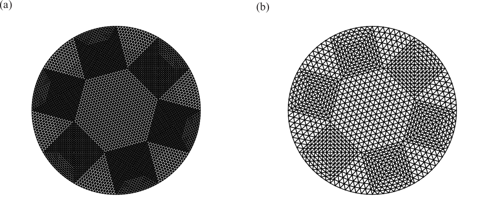
Figure 1: The triangular finite element meshes used for solving Poisson’s equation in the simulation of Jobelin vortex with a Dirichlet boundary condition. a After one level coarsening $(k=1)$, 4705 nodes and 9216 elements; b After two levels coarsening $(k=2)$, 1201 nodes and 2304 elements.

Tables 7–8 list the discrete error norms for the velocity, pressure, and pressure gradient fields as well as speedup factors, respectively, for RCGP and NCGP at time $t=­1$. Considering the 36864:36864 grid resolution, after two levels $(k=2)$ of the Poisson grid coarsening, the minimum speedup gained is equal to 3.943 and belongs to NCGP, whereas the maximum speedup achieved is equal to 102.715 and occurs in RCGP. To more precisely discuss the speedup factors, the relevant quantities are reported in detail. The computational times for the performed simulations using RCGP are: 61044.8, 13281.0, and 594.31, respectively for $k=0$ (36864:36864), $k=1$ (36864:9216), and $k=2$ (36864:2304), while the same simulation using NCGP takes: 60831.7, 27414.0, and 15427.7, respectively for $k=0$, $k=1$, and $k=2$. On the other hand, the computational cost devoted to the Poisson equation solver in the RCGP scheme are: 60839.9, 13076.2, and 389.28, respectively for $k=0$, $k=1$, and $k=2$, while obtaining the solution of Poisson’s equation performed by the NCGP method takes: 60626.4, 26991.2, and 14105.3, respectively, for $k=0$, $k=1$, and $k=2$. Even in unstructured grids, the RCGP system keeps the accuracy of the pressure field to an excellent degree, as can be seen from Table 7. Interestingly, the computational cost paid to this goal becomes inexpensive and high saving in CPU time is gained. The NCGP tool, in contrast, preserves the accuracy of the pressure and velocity fields in a lower order and with lower speedups. A visual demonstration of this interpretation is displayed in Figs. 2–3.

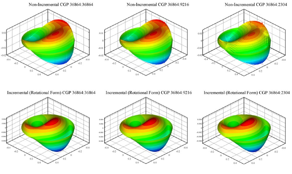
Figure 2: Distribution of point-wise velocity error for Jobelin vortex problem with Dirichlet boundary conditions at $t=1$. Labels in the form of $M:N$ indicate the grid resolution of the advection-diffusion solver, $M$ elements, and the Poisson equation, $N$ elements.

Figure 3: Distribution of point-wise pressure error for Jobelin vortex problem with Dirichlet boundary conditions at $t=1$. Labels in the form of $M:N$ indicate the grid resolution of the advection-diffusion solver, $M$ elements, and the Poisson equation, $N$ elements.

Table 7: Error norms and relative speedups for different grid resolutions of the Jobelin vortex problem with Dirichlet boundary conditions using the incremental projection method (rotational form) at $t=1$. $M:N$ represents the grid resolution of the advection-diffusion solver ($M$ elements) and Poisson’s equation ($N$ elements).

$k$	Resolution	$\|\textbf{{u}}\|_{L^{2}(V)}$	$\|p\|_{L^{2}(V)}$	$\|\textbf{G}$P$\|_{L^{2}(V)}$	Speedup
0	36864:36864	1.97531E$-$8	5.19843E$-$6	2.37525E$-$10	1.000
1	36864:9216	1.97531E$-$8	5.19843E$-$6	2.37525E$-$10	4.596
2	36864:2304	1.97531E$-$8	5.19843E$-$6	2.37525E$-$10	102.715
0	9216:9216	8.07724E$-$8	2.18577E$-$5	4.83658E$-$9	1.000
1	9216:2304	8.08305E$-$8	2.18579E$-$5	4.83861E$-$9	2.155
0	2304: 2304	3.16102E$-$7	8.62595E$-$5	7.51999E$-$8	1.000

Table 8: Error norms and relative speedups for different grid resolutions of the Jobelin vortex problem with Dirichlet boundary conditions using the non-incremental projection method at $t=1$. $M:N$ represents the grid resolution of the advection-diffusion solver ($M$ elements) and Poisson’s equation ($N$ elements).

$k$	Resolution	$\|\textbf{{u}}\|_{L^{2}(V)}$	$\|p\|_{L^{2}(V)}$	$\|\textbf{G}$P$\|_{L^{2}(V)}$	Speedup
0	36864:36864	5.52553E$-$8	5.42703E$-$6	3.06539E$-$10	1.000
1	36864:9216	5.53430E$-$8	5.42704E$-$6	3.06676E$-$10	2.219
2	36864:2304	5.56868E$-$8	5.42706E$-$6	3.06683E$-$10	3.943
0	9216:9216	2.19621E$-$7	2.34661E$-$5	1.28570E$-$8	1.000
1	9216:2304	2.20984E$-$7	2.34663E$-$5	1.28648E$-$8	2.056
0	2304: 2304	8.68060E$-$7	0.000110098	4.05365E$-$7	1.000

Figure 2 and Figure 3 show the associated point-wise error distributions, respectively, for the velocity and pressure variables using the NCGP and RCGP simulations. The general resultant patterns of point-wise error distribution of NCGP and RCGP over the velocity domains are identical. However, NCGP calculations lead to higher infinity norms in comparison with RCGP. Moreover, the RCGP procedure produces identical velocity noise patterns for $k=0$, $k=1$, and $k=2$. As shown in Fig. 3, the point-wise error distribution pattern of NCGP over the pressure domain is completely different in comparison with those executed by RCGP. As depicted in Fig.2, because the NCGP module is disable to remove resulting artificial layers from the artificial Neumann pressure boundary conditions, the maximum velocity noise is observed on its circular domain boundaries, while these layers disappear in velocity domains simulated by RCGP for all the presented resolutions.

It is worthwhile to note that SCGP is also successful in terms of accuracy and speedup levels. However, its performance is similar to RCGP from the both aspects and that is why we only presented the results computed by RCGP in this section.

4 Conclusions and future directions

The contribution of the CGP methodology to pressure correction schemes is to accelerate the computations while preserving the accuracy of the pressure and velocity fields by evolving the nonlinear advection-diffusion equation on a fine grid and solving the linear Poisson equation on a corresponding coarsened grid. For the first time in this article, a CGP mechanism is implemented in standard/rotational incremental pressure correctio methods. Here, Poisson’s equation is solved on a coarsened mesh for an intermediate variable related to the pressure field. Hence, in contrast with the non incremental procedure, the resolution of the pressure field remains unchanged.

Three different standard test cases were solved in order to examine the performance of the proposed CGP technique: The Taylor-Green vortex with velocity Dirichlet boundary conditions [14], the Jobelin vortex with open boundary conditions [12], and the Jobelin vortex with Dirichlet boundary conditions [12]. The speedup factors ranged from 1.248 to 102.715. We observed the minimum speedup in the Taylor-Green vortex with Dirichlet boundary conditions [14] with the standard form of the incremental pressure correction scheme, while the maximum speedup belonged to the Jobelin vortex with Dirichlet boundary conditions [12] with the rotational form.

In terms of the accuracy level, generally the velocity, pressure, and pressure gradient fields, for one, two, and three Poisson grid coarsening levels maintained excellent agreement with those performed on full fine scale grid resolutions. In the presence of open boundary conditions, the coarse-grid-projection incremental form of pressure correction schemes obtained velocity and pressure norms approximately identical to those computed using full fine scale simulations. For velocity Dirichlet boundary conditions as well as irregular physical domains, the coarse-grid projection incremental form of pressure correction methods achieved significant speedup factors while preserving the accuracy of both the velocity and pressure fields.

In this article, we used the method of manufactured solutions. We considered a low Reynolds number of $Re=10$. Generally, the SCGP and RCGP techniques were prosperous. Note that there is an important difference between the non-incremental and incremental correction formulations. In the incremental techniques, the Poisson equation is solved for an intermediate variable relevant to the pressure. This feature enables the CGP method to preserve the pressure accuracy level high even for three Poisson grid coarsening levels, whereas this precision is not obtained in the incorporation of the CGP mechanism and the non-incremental pressure projection method. On the other hand, incremental forms force the pressure gradient term to the momentum balance. The pressure gradient coming from CGP still experiences artificial fluctuations.

Although the magnitude of these fluctuations is low, we need to filter them at high-Reynolds number implementations of RCGP and SCGP methodologies. Thus, designing efficient filters to reach this goal is the topic of our future research.

Another objective of a future study is to apply a CGP method to the Nodal Discontinuous Galerkin (NDG) [23] spatial discretization scheme. From a grid resolution point of view, in the NDG approach the polynomial order of an element demonstrates its grid resolution. Hence, coarsening a mesh can take a new shape. Instead of decreasing the number of elements, one may decrease the polynomial order of the discretized space. In this way, incorporation of the CGP methodology and the NDG scheme for incompressible flow simulations means solving the momentum balance and the Poisson equations on grids with the same number of elements but with different polynomial orders for each mesh. Accordingly, the advection-diffusion grid takes higher order polynomials in comparison with the Poisson equation one. In this case, defining novel restriction, prolongation, divergence and Laplacian operators as well as designing efficient data structures for nodal connectivity between the advection-diffusion and the pressure grids should be investigated.

- (1) Chorin AJ (1968) Numerical solution of the Navier-Stokes equations. Mathematics of computation 22 (104):745-762
- (2) Temam R (1969) Sur l’approximation de la solution des équations de Navier-Stokes par la méthode des pas fractionnaires (II). Archive for Rational Mechanics and Analysis 33 (5):377-385
- (3) Guermond J-L, Minev P, Shen J (2005) Error analysis of pressure-correction schemes for the time-dependent Stokes equations with open boundary conditions. SIAM Journal on Numerical Analysis 43 (1):239-258
- (4) Lentine M, Zheng W, Fedkiw R A novel algorithm for incompressible flow using only a coarse grid projection. In: ACM Transactions on Graphics (TOG), 2010. vol 4. ACM, p 114
- (5) San O, Staples AE (2013) A coarse-grid projection method for accelerating incompressible flow computations. Journal of Computational Physics 233:480-508
- (6) San O, Staples AE (2013) An efficient coarse grid projection method for quasigeostrophic models of large-scale ocean circulation. International Journal for Multiscale Computational Engineering 11 (5)
- (7) Jin M, Liu W, Chen Q (2014) Accelerating fast fluid dynamics with a coarse-grid projection scheme. HVAC&R Research 20 (8):932-943
- (8) Kashefi A, Staples AE (2016) Acceleration of incremental-pressure-correction incompressible flow computations using a coarse-grid projection method. Bulletin of the American Physical Society 61 https://meetings.aps.org/Meeting/DFD15/Session/R7.4
- (9) Kashefi A, Staples AE (2018) A finite-element coarse-grid projection method for incompressible flow simulations. Advances in Computational Mathematics 44 (4):1063-1090
- (10) Kashefi A (2018) Transport of passive scalars in incompressible flows using a coarse-grid projection method. arXiv:1802.09744 [physics.comp-ph]
- (11) Kashefi A (2018) Coarse grid projection methodology: A partial mesh refinement tool for incompressible flow simulations. arXiv:1803.10340v1 [physics.comp-ph]
- (12) Jobelin M, Lapuerta C, Latché J-C, Angot P, Piar B (2006) A finite element penalty-projection method for incompressible flows. Journal of Computational Physics 217 (2):502-518
- (13) Timmermans L, Minev P, Van De Vosse F (1996) An approximate projection scheme for incompressible flow using spectral elements. International journal for numerical methods in fluids 22 (7):673-688
- (14) Taylor G, Green A (1937) Mechanism of the production of small eddies from large ones. Proceedings of the Royal Society of London Series A, Mathematical and Physical Sciences 158 (895):499-521
- (15) Wanner G, Hairer E (1991) Solving ordinary differential equations II, vol 1. Springer-Verlag, Berlin
- (16) Reddy JN (1993) An introduction to the finite element method, vol 2. vol 2.2. McGraw-Hill New York
- (17) Brezzi F (1974) On the existence, uniqueness and approximation of saddle-point problems arising from Lagrangian multipliers. Revue française d’automatique, informatique, recherche opérationnelle Analyse numérique 8 (2):129-151
- (18) Babuška I (1973) The finite element method with Lagrangian multipliers. Numerische Mathematik 20 (3):179-192
- (19) Sampath RS, Biros G (2010) A parallel geometric multigrid method for finite elements on octree meshes. SIAM Journal on Scientific Computing 32 (3):1361-1392
- (20) Saad Y, Schultz MH (1986) GMRES: A generalized minimal residual algorithm for solving nonsymmetric linear systems. SIAM Journal on scientific and statistical computing 7 (3):856-869
- (21) Van der Vorst HA (2003) Iterative Krylov methods for large linear systems, vol 13. Cambridge University Press
- (22) Geuzaine C, Remacle JF (2009) Gmsh: A 3‐D finite element mesh generator with built‐in pre‐and post‐processing facilities. International Journal for Numerical Methods in Engineering 79 (11):1309-1331
- (23) Hesthaven JS, Warburton T (2007) Nodal Discontinuous Galerkin Methods: Algorithms, Analysis, and Applications, Springer Science & Business Media