Minor loops of the Dahl and LuGre models

Abstract

Hysteresis is a special type of behavior encountered in physical systems: in a hysteretic system, when the input is periodic and varies slowly, the steady-state part of the output-versus-input graph becomes a loop called hysteresis loop. In the presence of perturbed inputs, this hysteresis loop presents small lobes called minor loops that are located inside a larger curve called major loop. The study of minor loops is being increasingly popular since it leads to a quantification of the loss of energy. The aim of the present paper is to give an explicit analytic expression of the minor loops of the LuGre and the Dahl models of dynamic dry friction.

1 Introduction

Hysteresis is a nonlinear phenomenon observed in some physical systems under low-frequency excitations. It appears in many areas as biology, electronics, ferroelasticity, magnetism, mechanics or optics [3, 4, 14, 16, 22]. This phenomenon is currently classified into two categories: rate independent (RI) and rate dependent (RD) hysteresis. For RI hysteresis, the output-versus-input graph of the hysteresis system does not change with the frequency of the input signal. This is the case for example of the Bouc-Wen or the Preisach models, see [13] and [17] respectively. For RD hysteresis, the output-versus-input graph of the hysteresis system may change with the frequency, but it converges in some sense to a fixed loop called the hysteresis loop when the frequency goes to zero. This is the case for example of the LuGre model and the semilinear Duhem model, see [19] and [12, 20] respectively. Research in the field of hysteresis has focused mainly on the study of rate-independent hysteresis, and it is only in the last 15 years that the importance of rate-dependent phenomena has been acknowledged, and it constitutes a challenge by itself.

The recent years have witnessed a growing interest in a phenomenon that appears in hysteretic systems under perturbed periodic signals: the hysteresis loop shows to be composed of a big cycle called major loop, and one or several small lobes called minor loops located inside the major loop. Figure 1 shows the hysteresis loop of a magnetic system when the input is the one of Figure 2, see [10] for instance.

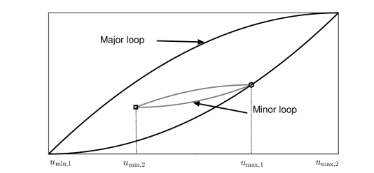
Figure 1: Hysteresis loop of a magnetic system with the input of Figure 2. Black: major loop. Grey: minor loop.

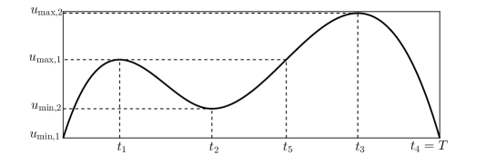
Figure 2: A bimodal $T$–periodic input $u(t)$ versus $t$.

This interest in the study of minors loops is due in part to the fact that minor loops are related to a loss of energy, see [24] for instance.

From a formal point of view, minor loops have been studied mainly in relation with the Preisach model [17, p.19]. Apart from [12, Sections 10, 11.9] we are not aware of any mathematical analysis of minor loops of hysteresis systems given by differential equations.

The aim of the present paper is to fill this void by providing an explicit analytic description of the minor loops of the Dahl and the LuGre models.

The Dahl model is an idealization of dynamic dry friction proposed by Dahl in 1976 [6]. This model relates an input displacement $u$ to an output force $y$ as

$$y(t)=F_{c}\,w(t),$$

$$\dot{w}(t)=\rho\big{(}\dot{u}(t)-|\dot{u}(t)|w(t)\big{)},$$

$$-1\leq w(0)\leq 1,$$

where $w$ is an internal state and $\rho>0$, $F_{c}>0$ are constants. A good introductory text on the relationship between the Dahl model and the Coulomb model of dry friction may be found in [8].

The LuGre model is a generalization of the Dahl model introduced in 1995 to include the Stribeck effect, that is the decrease of friction at low velocities [5]. The LuGre model is given by [2]:

$$\begin{array}[]{lcl}\dot{x}\left(t\right)&=&-\sigma_{0}\dfrac{|\dot{u}(t)|}{g\big{(}\dot{u}(t)\big{)}}x\left(t\right)+\dot{u}(t),\\ x(0)&=&x_{0},\\ F\left(t\right)&=&\sigma_{0}x(t)+\sigma_{1}\dot{x}(t)+f\big{(}\dot{u}(t)\big{)},\end{array}$$ (1)

where $t\geq 0$ denotes time; the parameters $\sigma_{0}>0$ and $\sigma_{1}>0$ are respectively the stiffness and the microscopic damping friction coefficients; the function $g$ is continuous with $g\left(\vartheta\right)>0$ for all $\vartheta\in\mathbb{R}$ and it represents the macrodamping friction ; $x(t)\in\mathbb{R}$ is the average deflection of the bristles; $x_{0}\in\mathbb{R}$ is the initial state; $u(t)$ is the relative displacement and is the input of the system; $F(t)$ is the friction force and is the output of the system; and $f$ is continuous and such that $f(0)=0$. When the function $g$ is constant, $\sigma_{1}=0$ and $f$ is the zero function, the system (1) reduces to the Dahl model. Both the LuGre and the Dahl models have been used in various applications, see for instance [1, 7, 9].

The main contribution of this paper is Theorem A which is stated in Section 3.1. This theorem provides the analytic description of the minor loop of the LuGre and Dahl models when the input is bimodal like in Figure 2.

The paper is organized as follows: Section 2 provides the mathematical notation used in the text. In Section 3 we present and prove the main result which is the analytical description of the minor loop of the LuGre and Dahl models. Section 4 has a pedagogical interest: using numerical simulations we present examples that illustrate the constructive process which leads to the hysteresis and minor loops. Some of these examples are aimed for the reader who may not be familiar with the technicalities that underline the methodology used here. The conclusions are provided in Section 5.

2 Mathematical notation

We say that a subset of $\mathbb{R}$ is measurable when it is Lebesgue measurable. Consider a function $g:I\subseteq\mathbb{R}\rightarrow\mathbb{R}$ where $I$ is an interval. We say that $g$ is measurable if $g^{-1}(B)$ is a measurable set for any set $B$ in the Borel algebra of $\mathbb{R}$ or, equivalently, if $\{x\in I:\,g(x)>a\}$ is a measurable set for all $a\in\mathbb{R}$, [21, 23]. For a measurable function $g:I\rightarrow\mathbb{R}$, $\|g\|$ denotes the essential supremum of the function $|g|$ where $|\cdot|$ is the absolute value.

We recall that $\mathcal{C}^{0}(\mathbb{R}^{+},\mathbb{R})$ denotes the space of continuous functions defined from $\mathbb{R}+$ to $\mathbb{R}$ endowed with the norm $\|\cdot\|$. Also $W^{1;\infty}(\mathbb{R}^{+},\mathbb{R})$ denotes the Sobolev space of absolutely continuous functions $u:\mathbb{R}^{+}\rightarrow\mathbb{R}$. For this class of functions, the derivative $\dot{u}$ is measurable, and we have $\|u\|<\infty$, $\|\dot{u}\|<\infty$. Endowed with the norm $\|u\|_{1,\infty}=\max\left(\|u\|,\|\dot{u}\|\right)$, $W^{1;\infty}(\mathbb{R}^{+},\mathbb{R})$ is a Banach space [15, pp. 280–281]. Finally, $L^{\infty}(I,\mathbb{R})$ denotes the Banach space of measurable functions $u:I\rightarrow\mathbb{R}$ such that $\|u\|<\infty$, endowed with the norm $\|\cdot\|$. For $T>0$ we define $\Omega_{T}$ as the set of all $T$–periodic functions $u\in W^{1;\infty}(\mathbb{R}^{+},\mathbb{R})$.

3 Main result

3.1 Statement of the main result

We consider the LuGre model (1) with an input $u\in W^{1;\infty}(\mathbb{R}^{+},\mathbb{R})$. In [19] it is proved that for all $x_{0}\in\mathbb{R}$, the differential equation (1) has a unique Carathéodory solution $x\in W^{1;\infty}(\mathbb{R}^{+},\mathbb{R})$ and that $F\in L^{\infty}(\mathbb{R}^{+},\mathbb{R})$.

To present the main result of this work which is the analytic characterization of the minor loop we define formally the set of bimodal inputs needed to generate this minor loop.

Definition 1.

Let $u_{\min,1},u_{\min,2},u_{\max,1},u_{\max,2}\in\mathbb{R}$ be such that $u_{\min,1}\leq u_{\min,2}<u_{\max,1}\leq u_{\max,2}$ and at least one of the following holds: $u_{\min,1}\neq u_{\min,2}$ or $u_{\max,1}\neq u_{\max,2}$. Let $t_{1},t_{2},t_{3},t_{4}\in\mathbb{R}^{+}$ be such that $0<t_{1}<t_{2}<t_{3}<t_{4}$. We define $\mathbb{M}_{u_{\min,1},u_{\min,2},u_{\max,1},u_{\max,2},t_{1},t_{2},t_{3},t_{4}}$ as the set of all functions $u\in\Omega_{t_{4}}$ such that $u$ is strictly increasing on the interval $[0,t_{1}]$, strictly decreasing on the interval $[t_{1},t_{2}]$, strictly increasing on the interval $[t_{2},t_{3}]$, strictly decreasing on the interval $[t_{3},t_{4}]$; and $u(0)=u_{\min,1}$, $u(t_{1})=u_{\max,1}$, $u(t_{2})=u_{\min,2}$, $u(t_{3})=u_{\max,2}$, $u(t_{4})=u(0)$.

Theorem A.

Let us consider the LuGre model given by Equations (1) with an input $u\in\mathbb{M}_{u_{\min,1},u_{\min,2},u_{\max,1},u_{\max,2},t_{1},t_{2},t_{3},t_{4}}$. Then the following statements hold:

1. The hysteresis loop that corresponds to the input $u$ is the set

   $$G_{u}^{\circ}=\big{\{}\big{(}\psi_{u}(t),y^{\circ}(t)\big{)}\in\mathbb{R}^{2},\,t\in[0,\varrho_{4}]\big{\}},$$

   where $y^{\circ}$ is given by

   $$y^{\circ}(t)=\mathrm{e}^{-\frac{\sigma_{0}}{g(0)}(t-\varrho_{i})}\left(y^{\circ}(\varrho_{i})-g(0)\left[\mathrm{e}^{\frac{\sigma_{0}}{g(0)}(t-\varrho_{i})}-1\right]\right),\mbox{ for }t\in[\varrho_{i},\varrho_{i+1}]$$

   and $i\in\{0,1,2,3\}$, and where

   $$y^{\circ}(0)=g(0)\,\frac{\mathrm{e}^{-\frac{\sigma_{0}}{g(0)}\varrho_{4}}}{1-\mathrm{e}^{-\frac{\sigma_{0}}{g(0)}\varrho_{4}}}\left(2\mathrm{e}^{\frac{\sigma_{0}}{g(0)}\varrho_{1}}-2\mathrm{e}^{\frac{\sigma_{0}}{g(0)}\varrho_{2}}+2\mathrm{e}^{\frac{\sigma_{0}}{g(0)}\varrho_{3}}-\mathrm{e}^{\frac{\sigma_{0}}{g(0)}\varrho_{4}}-1\right)\mbox{ and }$$

   $$y^{\circ}(\varrho_{i})=\mathrm{e}^{-\frac{\sigma_{0}}{g(0)}(\varrho_{i}-\varrho_{i-1})}\left(y^{\circ}(\varrho_{i-1})+g(0)\left[\mathrm{e}^{\frac{\sigma_{0}}{g(0)}(\varrho_{i}-\varrho_{i-1})}-1\right]\right)\mbox{ for }i\in\{1,2,3,4\};$$

   and $\psi_{u}$ is given by

   $$\psi_{u}(t)=\begin{cases}\begin{array}[]{ll}t+u_{\min,1}&\text{for }t\in[0,\varrho_{1}],\\ -t+\varrho_{1}+u_{\max,1}&\text{for }t\in[\varrho_{1},\varrho_{2}],\\ t-\varrho_{2}+u_{\min,2}&\text{for }t\in[\varrho_{2},\varrho_{3}],\\ -t+\varrho_{3}+u_{\max,2}&\text{for }t\in[\varrho_{3},\varrho_{4}],\end{array}\end{cases}$$

   being $\varrho_{0}=0$, $\varrho_{1}=\;u_{\max,1}-u_{\min,1}>0,$ $\varrho_{2}=\;\varrho_{1}+u_{\max,1}-u_{\min,2}>\varrho_{1},$ $\varrho_{3}=\;\varrho_{2}+u_{\max,2}-u_{\min,2}>\varrho_{2},$ and $\varrho_{4}=\;\varrho_{3}+u_{\max,2}-u_{\min,1}>\varrho_{3}$.

2. The minor loop that corresponds to the input $u$ is the set

   $$\mathcal{N}_{u}=\big{\{}\big{(}\psi_{u}(t),y^{\circ}(t)\big{)},t\in[\varrho_{1},\varrho_{5}]\big{\}},$$

   where $\varrho_{5}=u_{\max,1}-u_{\min,2}+\varrho_{2}\in(\varrho_{2},\varrho_{3}]$.

Comment. Observe that the sets $G^{\circ}_{u}$ and $\mathcal{N}_{u}$ are the geometric loci of parametrized curves. Theorem A, thus, gives an explicit parametrization of these curves.

3.2 Proof of Theorem A

The proof of Theorem A is done is three steps:

1. The hysteresis loop of the LuGre and the Dahl models are derived in Section 3.2.1.

2. A normalized input is presented in Section 3.2.2.

3. The determination of the equations of the minor loop is done in Section 3.2.3.

3.2.1 Hysteresis loop of the LuGre and the Dahl models

To prove Theorem A and therefore to derive the explicit expression of the hysteresis loop of the LuGre and the Dahl models, we follow the methodology presented in [11, 19]. In this section we recall and adapt the main steps of this methodology. The reader unfamiliar with this theoretical framework is first referred to Example 1 in Section 4.1.

Let $u\in\mathbb{M}_{u_{\min,1},u_{\min,2},u_{\max,1},u_{\max,2},t_{1},t_{2},t_{3},t_{4}}$ and take $T=t_{4}$. Also, take $\gamma\in(0,\infty)$ and consider the linear time-scale change $s_{\gamma}:\mathbb{R}\rightarrow\mathbb{R}$ defined by $s_{\gamma}(t)=t/\gamma$ for all $t\in\mathbb{R}$. Then $u\circ s_{\gamma}$ is $\gamma T$–periodic.

The system (1) for which the input is $u\circ s_{\gamma}$ can be written as

$$\dot{x}_{\gamma}\left(t\right) = -\sigma_{0}\frac{\big{|}\dot{\mathop{\vbox{\halign{#\cr\kern 2.15277pt\cr$\braceld\leaders\vrule height=0.39998pt,depth=0.0pt\hfill\bracerd$\crcr\kern 3.01385pt\nointerlineskip\cr$\hfil\displaystyle{{u\circ s_{\gamma}}}\hfil$\crcr}}}\limits}(t)\big{|}}{g\big{(}\dot{\mathop{\vbox{\halign{#\cr\kern 2.15277pt\cr$\braceld\leaders\vrule height=0.39998pt,depth=0.0pt\hfill\bracerd$\crcr\kern 3.01385pt\nointerlineskip\cr$\hfil\displaystyle{u\circ s_{\gamma}}\hfil$\crcr}}}\limits}(t)\big{)}}x_{\gamma}\left(t\right)+\dot{\mathop{\vbox{\halign{#\cr\kern 2.15277pt\cr$\braceld\leaders\vrule height=0.39998pt,depth=0.0pt\hfill\bracerd$\crcr\kern 3.01385pt\nointerlineskip\cr$\hfil\displaystyle{{u\circ s_{\gamma}}}\hfil$\crcr}}}\limits}\left(t\right),\text{ for almost all }t\in\mathbb{R}^{+},$$

$$x_{\gamma}(0) = x_{0},$$

$$F_{\gamma}\left(t\right) = \sigma_{0}x_{\gamma}\left(t\right)+\sigma_{1}\dot{x}_{\gamma}(t)+f\big{(}\dot{\mathop{\vbox{\halign{#\cr\kern 2.15277pt\cr$\braceld\leaders\vrule height=0.39998pt,depth=0.0pt\hfill\bracerd$\crcr\kern 3.01385pt\nointerlineskip\cr$\hfil\displaystyle{{u\circ s_{\gamma}}}\hfil$\crcr}}}\limits}(t)\big{)},\text{ for almost all }t\in\mathbb{R}^{+}.$$

On the other hand,

$$\dot{\mathop{\vbox{\halign{#\cr\kern 2.15277pt\cr$\braceld\leaders\vrule height=0.39998pt,depth=0.0pt\hfill\bracerd$\crcr\kern 3.01385pt\nointerlineskip\cr$\hfil\displaystyle{{u\circ s_{\gamma}}}\hfil$\crcr}}}\limits}(t)=\dot{u}\big{(}s_{\gamma}(t)\big{)}\cdot\dot{s}_{\gamma}(t)=\dot{u}\left(\frac{t}{\gamma}\right)\cdot\frac{1}{\gamma},$$

so that we get

$$\dot{x}_{\gamma}\left(t\right) = -\sigma_{0}\frac{\left|\frac{1}{\gamma}\dot{u}\left(\frac{t}{\gamma}\right)\right|}{g\left(\frac{1}{\gamma}\dot{u}\left(\frac{t}{\gamma}\right)\right)}x_{\gamma}\left(t\right)+\frac{1}{\gamma}\dot{u}\left(\frac{t}{\gamma}\right),\text{ for almost all }t\in\mathbb{R}^{+},$$

$$x_{\gamma}(0) = x_{0},$$

$$F_{\gamma}\left(t\right) = \sigma_{0}x_{\gamma}\left(t\right)+\sigma_{1}\dot{x}_{\gamma}(t)+f\left(\frac{1}{\gamma}\dot{u}\left(\frac{t}{\gamma}\right)\right),\text{ for almost all }t\in\mathbb{R}^{+}.$$

Now, defining $\nu=t/\gamma$ we rewrite these relations in terms of $\nu$ obtaining

$$\begin{split}\gamma\dot{x}_{\gamma}\left(\gamma\nu\right)&=-\sigma_{0}\frac{|\dot{u}(\nu)|}{g\left(\frac{1}{\gamma}\dot{u}(\nu)\right)}x_{\gamma}(\gamma\nu)+\dot{u}(\nu),\text{ for almost all }\nu\in\mathbb{R}^{+},\\ x_{\gamma}(0)&=x_{0},\\ F_{\gamma}(\gamma\nu)&=\sigma_{0}x_{\gamma}(\gamma\nu)+\sigma_{1}\dot{x}_{\gamma}(\gamma\nu)+f\left(\frac{1}{\gamma}\dot{u}(\nu)\right),\text{ for almost all }\nu\in\mathbb{R}^{+}.\end{split}$$ (4)

We define the function $z_{\gamma}$ by the relation $z_{\gamma}=x_{\gamma}\circ s_{1/\gamma}$ so that

$$\dot{z}_{\gamma}(\nu)=\dot{x}_{\gamma}\big{(}s_{1/\gamma}(\nu)\big{)}\cdot\dot{s}_{1/\gamma}(\nu)=\dot{x}_{\gamma}(\gamma\nu)\cdot\gamma.$$

Substituting in (4) provides:

$$\begin{split}&\dot{z}_{\gamma}\left(t\right)=-\sigma_{0}\frac{|\dot{u}(t)|}{g\left(\frac{\dot{u}(t)}{\gamma}\right)}z_{\gamma}(t)+\dot{u}(t),\text{ for almost all }t\in\mathbb{R}^{+},\\ &z_{\gamma}(0)=x_{0},\\ &y_{\gamma}(t)=\sigma_{0}z_{\gamma}(t)+\frac{\sigma_{1}}{\gamma}\dot{z}_{\gamma}(t)+f\left(\frac{\dot{u}(t)}{\gamma}\right),\text{ for almost all }t\in\mathbb{R}^{+},\end{split}$$ (5)

where $y_{\gamma}=F_{\gamma}\circ s_{1/\gamma}$.

For a given $\gamma>0$, the corresponding output-versus-input graph is the set $G_{u\circ s_{\gamma}}=\big{\{}\big{(}u\circ s_{\gamma}(t),F_{\gamma}(t)\big{)},t\geq 0\big{\}}=\big{\{}\big{(}u(t),F_{\gamma}\circ s_{1/\gamma}(t)=y_{\gamma}(t)\big{)},t\geq 0\big{\}}$. The hysteresis loop of system (5) is the output-versus-input graph obtained for very slow inputs (that is when $\gamma\rightarrow\infty$) in steady state. The next result, which is a straightforward combination of [18, Proposition 5] and [19, Theorem 9], describes the result of this convergence process.

Theorem 2 ([18, 19]).

The following statements hold:

1. The sequence of functions $(y_{\gamma})_{\gamma>0}$ converges in the space $L^{\infty}(\mathbb{R}^{+},\mathbb{R})$ as $\gamma\rightarrow\infty$. Denote $y^{\star}_{u}=\lim_{\gamma\rightarrow\infty}y_{\gamma}$, then for all $t\in\mathbb{R}^{+}$ we have

   $$y^{\star}_{u}(t) = \sigma_{0}\mathrm{e}^{-\frac{\sigma_{0}}{g(0)}\rho_{u}(t)}\left(x_{0}+\int_{0}^{t}\mathrm{e}^{\frac{\sigma_{0}}{g(0)}\rho_{u}(\tau)}\dot{u}(\tau)d\tau\right),$$ (6)

   $$\rho_{u}(t) = \int_{0}^{t}|\dot{u}(\tau)|d\tau.$$ (7)

2. For any $k\in\mathbb{N}$ define the function $y^{\star}_{u,k}\in L^{\infty}\big{(}[0,T],\mathbb{R}\big{)}$ by $y^{\star}_{u,k}(t)=y^{\star}_{u}(t+kT)$, for all $t\in[0,T]$. The sequence of functions $(y^{\star}_{u,k})_{k\in\mathbb{N}}$ converges in the space $L^{\infty}\big{(}[0,T],\mathbb{R}\big{)}$ as $k\rightarrow\infty$. Denote $y^{\circ}_{u}=\lim_{k\rightarrow\infty}y^{\star}_{u,k}$, then

   $$y^{\circ}_{u}(t)=\sigma_{0}\mathrm{e}^{-\frac{\sigma_{0}}{g(0)}\rho_{u}(t)}\left(\frac{y^{\circ}_{u}(0)}{\sigma_{0}}+\int_{0}^{t}\mathrm{e}^{\frac{\sigma_{0}}{g(0)}\rho_{u}(\tau)}\dot{u}(\tau)d\tau\right)\mbox{ for all }t\in[0,T].$$ (8)

   Moreover, $y^{\circ}_{u}(T)=y^{\circ}_{u}(0)$.

Statement (a) implies that the graphs $G_{u\circ s_{\gamma}}$ converge in a sense precised in [11, Lemma 9] to the graph $G^{\star}_{u}=\big{\{}\big{(}u(t),y^{\star}_{u}(t)\big{)},t\geq 0\big{\}}$ as $\gamma\rightarrow\infty$. The hysteresis loop is given by the “steady state” of the parametrized curve $G^{\star}_{u}$ which by statement (b) is the set

$$G_{u}^{\circ}=\big{\{}\big{(}u(t),y^{\circ}_{u}(t)\big{)},t\in[0,T]\big{\}}.$$ (9)

Moreover, Theorem 2 (b) gives

$$y^{\circ}_{u}(T) = \sigma_{0}\mathrm{e}^{-\frac{\sigma_{0}}{g(0)}\rho_{u}(T)}\left(\frac{y^{\circ}_{u}(0)}{\sigma_{0}}+\int_{0}^{T}\mathrm{e}^{\frac{\sigma_{0}}{g(0)}\rho_{u}(\tau)}\dot{u}(\tau)d\tau\right),$$

$$y^{\circ}_{u}(T) = y^{\circ}_{u}(0),$$

which leads to

$$y^{\circ}_{u}(0)=\frac{\sigma_{0}\mathrm{e}^{-\frac{\sigma_{0}}{g(0)}\rho_{u}(T)}\int_{0}^{T}\mathrm{e}^{\frac{\sigma_{0}}{g(0)}\rho_{u}(\tau)}\dot{u}(\tau)d\tau}{1-\mathrm{e}^{-\frac{\sigma_{0}}{g(0)}\rho_{u}(T)}}.$$ (10)

Equations (8) and (10) provide the analytical expression of the hysteresis loop (9). This expression includes both the major loop and the minor loop.

Observe that for the LuGre model neither $\sigma_{1}$ nor $f$ intervene in the equation of the hysteresis loop, and only the value $g(0)$ appears in this equation. Also note that Equations (8)–(10) are also valid for the Dahl model since the latter is a particular case of the LuGre model.

In Example 2 of Section 4.2 the reader can find a detailed illustration of the concepts presented in this section.

3.2.2 The normalized input

The hysteresis loop of the LuGre and the Dahl models is given in (9), and it is characterized by the function $y^{\circ}_{u}$ of Theorem 2 (b). Note that we are considering general input functions $u\in\mathbb{M}_{u_{\min,1},u_{\min,2},u_{\max,1},u_{\max,2},t_{1},t_{2},t_{3},t_{4}}$ that may not allow an explicit calculation of the integral present in Equation (8). To get an explicit calculation of that integral we follow the approach of [11] and [19] that leads to the explicit expression of the hysteresis loop by using the so-called normalized input $\psi_{u}$ associated to $u$. The use of the normalized input will give another parametrization of the curve in (9), an explicit one.

According to [11], the normalized input associated to $u$ is a piecewise-linear function $\psi_{u}\in W^{1;\infty}(\mathbb{R}^{+},\mathbb{R})$ that satisfies

$$\psi_{u}\big{(}\rho_{u}(t)\big{)}=u(t)\mbox{ for all }t\in\mathbb{R}^{+},$$ (11)

where $\rho_{u}(t)=\int_{0}^{t}|\dot{u}(\tau)|d\tau$ is the variation function of $u$. Note that $\rho_{u}$ is strictly increasing so that it is invertible, and $\rho_{u}^{-1}$ is also strictly increasing. From equation (11) it comes that $\psi_{u}=u\circ\rho_{u}^{-1}$ so that $\psi_{u}$ is strictly increasing on the interval $[0,\varrho_{1}]$, where $\varrho_{1}=\rho_{u}(t_{1})$. Thus $\dot{\psi}_{u}(\varrho)\geq 0$ when $\varrho\in(0,\varrho_{1})$ and $\dot{\psi}_{u}(\varrho)$ exists. On the other hand, by [11, Lemma 2], the set on which $\dot{\psi}_{u}$ is not defined or is different from $\pm 1$ has measure zero. Thus $\dot{\psi}_{u}(\varrho)=1$ for almost all $\varrho\in(0,\varrho_{1})$. Using the fact that $\psi_{u}$ is absolutely continuous we obtain from the Fundamental Theorem of Calculus that

$$\psi_{u}(\varrho)-\psi_{u}(0)=\int_{0}^{\varrho}\dot{\psi}_{u}(\tau)\,\text{d}\tau=\int_{0}^{\varrho}\text{d}\tau=\varrho,\text{ for all }\varrho\in[0,\varrho_{1}].$$

Taking into account that $\psi_{u}\big{(}\rho_{u}(0)\big{)}=u(0)$ it comes that $\psi_{u}(0)=u_{\min,1}$ so that

$$\psi_{u}(\varrho)=\varrho+u_{\min,1},\text{ for all }\varrho\in[0,\varrho_{1}].$$

The details for the intervals $[\varrho_{1},\varrho_{2}]$, $[\varrho_{2},\varrho_{3}]$, and $[\varrho_{3},\varrho_{4}]$ are given hereafter.

• By definition of $u$ we have that $u$ is strictly increasing on the interval $[0,t_{1}]$ so that

  $$\varrho_{1}=\rho_{u}(t_{1})=\int_{0}^{t_{1}}|\dot{u}(t)|\text{d}t=\int_{0}^{t_{1}}\dot{u}(t)\text{d}t=u(t_{1})-u(0)=u_{\max,1}-u_{\min,1}.$$

  Also, from $\psi_{u}(\varrho)=\varrho+u_{\min,1}$ for $\varrho\in[0,\varrho_{1}]$ we get

  $$\psi_{u}(\varrho_{1})=\varrho_{1}+u_{\min,1}=u_{\max,1}.$$

  Note that $\rho_{u}$ is strictly increasing so that it is invertible, and $\rho_{u}^{-1}$ is also strictly increasing. From equation (11) it comes that $\psi_{u}=u\circ\rho_{u}^{-1}$ so that $\psi_{u}$ is strictly decreasing on the interval $[\varrho_{1},\varrho_{2}]$, where $\varrho_{2}=\rho_{u}(t_{2})$. Thus $\dot{\psi}_{u}(\varrho)\leq 0$ when $\varrho\in(\varrho_{1},\varrho_{2})$ and $\dot{\psi}_{u}(\varrho)$ exists. On the other hand, by [11, Lemma 2], the set on which $\dot{\psi}_{u}$ is not defined or is different from $\pm 1$ has measure zero. Thus $\dot{\psi}_{u}(\varrho)=-1$ for almost all $\varrho\in(\varrho_{1},\varrho_{2})$. Using the fact that $\psi_{u}$ is absolutely continuous we obtain from the Fundamental Theorem of Calculus that

  $$\psi_{u}(\varrho)-\psi_{u}(\varrho_{1})=\int_{\varrho_{1}}^{\varrho}\dot{\psi}_{u}(\tau)\,\text{d}\tau=\int_{\varrho_{1}}^{\varrho}-1\;\text{d}\tau=\varrho_{1}-\varrho,\text{ for all }\varrho\in[\varrho_{1},\varrho_{2}],$$

  which leads to

  $$\psi_{u}(\varrho)=\psi_{u}(\varrho_{1})+\varrho_{1}-\varrho=u_{\max,1}+\varrho_{1}-\varrho.$$

• By definition of $u$ we have that $u$ is strictly decreasing on the interval $[t_{1},t_{2}]$ so that

  $$\varrho_{2} = \rho_{u}(t_{2})=\int_{0}^{t_{2}}|\dot{u}(t)|\text{d}t=\underbrace{\int_{0}^{t_{1}}|\dot{u}(t)|\text{d}t}_{\varrho_{1}}+\int_{t_{1}}^{t_{2}}-\dot{u}(t)\text{d}t$$

  $$= \varrho_{1}+u(t_{1})-u(t_{2})=\varrho_{1}+u_{\max,1}-u_{\min,2}.$$

  Also, from $\psi_{u}(\varrho)=u_{\max,1}+\varrho_{1}-\varrho$ for $\varrho\in[\varrho_{1},\varrho_{2}]$ we get

  $$\psi_{u}(\varrho_{2})=u_{\max,1}+\varrho_{1}-\varrho_{2}=u_{\min,2}.$$

  From equation (11) it comes that $\psi_{u}=u\circ\rho_{u}^{-1}$ so that $\psi_{u}$ is strictly increasing on the interval $[\varrho_{2},\varrho_{3}]$, where $\varrho_{3}=\rho_{u}(t_{3})$. Thus $\dot{\psi}_{u}(\varrho)\geq 0$ when $\varrho\in(\varrho_{2},\varrho_{3})$ and $\dot{\psi}_{u}(\varrho)$ exists. On the other hand, by [11, Lemma 2], the set on which $\dot{\psi}_{u}$ is not defined or is different from $\pm 1$ has measure zero. Thus $\dot{\psi}_{u}(\varrho)=1$ for almost all $\varrho\in(\varrho_{2},\varrho_{3})$. Using the fact that $\psi_{u}$ is absolutely continuous we obtain from the Fundamental Theorem of Calculus that

  $$\psi_{u}(\varrho)-\psi_{u}(\varrho_{2})=\int_{\varrho_{2}}^{\varrho}\dot{\psi}_{u}(\tau)\,\text{d}\tau=\int_{\varrho_{2}}^{\varrho}\text{d}\tau=\varrho-\varrho_{2},\text{ for all }\varrho\in[\varrho_{2},\varrho_{3}],$$

  which leads to

  $$\psi_{u}(\varrho)=\psi_{u}(\varrho_{2})+\varrho-\varrho_{2}=u_{\min,2}+\varrho-\varrho_{2}.$$

• By definition of $u$ we have that $u$ is strictly increasing on the interval $[t_{2},t_{3}]$ so that

  $$\varrho_{3} = \rho_{u}(t_{3})=\int_{0}^{t_{3}}|\dot{u}(t)|\text{d}t=\underbrace{\int_{0}^{t_{2}}|\dot{u}(t)|\text{d}t}_{\varrho_{2}}+\int_{t_{2}}^{t_{3}}\dot{u}(t)\text{d}t$$

  $$= \varrho_{2}+u(t_{3})-u(t_{2})=\varrho_{2}+u_{\max,2}-u_{\min,2}.$$

  Also, from $\psi_{u}(\varrho)=u_{\min,2}+\varrho-\varrho_{2}$ for $\varrho\in[\varrho_{2},\varrho_{3}]$ we get

  $$\psi_{u}(\varrho_{3})=u_{\min,2}+\varrho_{3}-\varrho_{2}=u_{\max,2}.$$

  From equation (11) it comes that $\psi_{u}=u\circ\rho_{u}^{-1}$ so that $\psi_{u}$ is strictly decreasing on the interval $[\varrho_{3},\varrho_{4}]$, where $\varrho_{4}=\rho_{u}(t_{4})$. Thus $\dot{\psi}_{u}(\varrho)\leq 0$ when $\varrho\in(\varrho_{3},\varrho_{4})$ and $\dot{\psi}_{u}(\varrho)$ exists. On the other hand, by [11, Lemma 2], the set on which $\dot{\psi}_{u}$ is not defined or is different from $\pm 1$ has measure zero. Thus $\dot{\psi}_{u}(\varrho)=-1$ for almost all $\varrho\in(\varrho_{3},\varrho_{4})$. Using the fact that $\psi_{u}$ is absolutely continuous we obtain from the Fundamental Theorem of Calculus that

  $$\psi_{u}(\varrho)-\psi_{u}(\varrho_{3})=\int_{\varrho_{3}}^{\varrho}\dot{\psi}_{u}(\tau)\,\text{d}\tau=\int_{\varrho_{3}}^{\varrho}-1\;\text{d}\tau=\varrho_{3}-\varrho,\text{ for all }\varrho\in[\varrho_{3},\varrho_{4}],$$

  which leads to

  $$\psi_{u}(\varrho)=\psi_{u}(\varrho_{3})+\varrho_{3}-\varrho=u_{\max,2}+\varrho_{3}-\varrho.$$

As a summary, we have

$$\psi_{u}(\varrho)=\begin{cases}\begin{array}[]{ll}\varrho+u_{\min,1}&\mbox{for }\varrho\in[0,\varrho_{1}],\\ -\varrho+\varrho_{1}+u_{\max,1}&\mbox{for }\rho\in[\varrho_{1},\varrho_{2}],\\ \varrho-\varrho_{2}+u_{\min,2}&\mbox{for }\varrho\in[\varrho_{2},\varrho_{3}],\\ -\varrho+\varrho_{3}+u_{\max,2}&\mbox{for }\varrho\in[\varrho_{3},\varrho_{4}],\end{array}\end{cases}$$ (12)

where $\varrho_{1}=\;u_{\max,1}-u_{\min,1}>0,$ $\varrho_{2}=\;\varrho_{1}+u_{\max,1}-u_{\min,2}>\varrho_{1},$ $\varrho_{3}=\;\varrho_{2}+u_{\max,2}-u_{\min,2}>\varrho_{2},$ and $\varrho_{4}=\;\varrho_{3}+u_{\max,2}-u_{\min,1}>\varrho_{3}$. The function $\psi_{u}$ is continuous and $\varrho_{4}$–periodic. Its graph in the interval $[0,\varrho_{4}]$ is displayed in Figure 3.

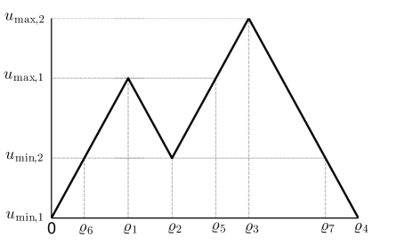
Figure 3: $\psi_{u}(\varrho)$ versus $\varrho$.

3.2.3 Analytic expression of the hysteresis and minor loops

Applying Theorem 2 (b) (Equation (8)) to the particular input $\psi_{u}$, and denoting for simplicity $y^{\circ}:=y^{\circ}_{\psi_{u}}$ we obtain that

$$y^{\circ}(\varrho)=\sigma_{0}\mathrm{e}^{-\frac{\sigma_{0}}{g(0)}\varrho}\left(\frac{y^{\circ}(0)}{\sigma_{0}}+\int_{0}^{\varrho}\mathrm{e}^{\frac{\sigma_{0}}{g(0)}\tau}\dot{\psi}_{u}(\tau)d\tau\right)\mbox{ for }\varrho\in[0,\varrho_{4}].$$

Since this expression can be explicitly integrated, we obtain

$$y^{\circ}(\varrho) = \mathrm{e}^{-\frac{\sigma_{0}}{g(0)}\varrho}\left(y^{\circ}(0)+g(0)\left[\mathrm{e}^{\frac{\sigma_{0}}{g(0)}\varrho}-1\right]\right)\mbox{ for }\varrho\in[0,\varrho_{1}],\mbox{ with }$$ (13)

$$y^{\circ}(0) = g(0)\,\frac{\mathrm{e}^{-\frac{\sigma_{0}}{g(0)}\varrho_{4}}}{1-\mathrm{e}^{-\frac{\sigma_{0}}{g(0)}\varrho_{4}}}\left(2\mathrm{e}^{\frac{\sigma_{0}}{g(0)}\varrho_{1}}-2\mathrm{e}^{\frac{\sigma_{0}}{g(0)}\varrho_{2}}+2\mathrm{e}^{\frac{\sigma_{0}}{g(0)}\varrho_{3}}-\mathrm{e}^{\frac{\sigma_{0}}{g(0)}\varrho_{4}}-1\right);$$

$$y^{\circ}(\varrho) = \mathrm{e}^{-\frac{\sigma_{0}}{g(0)}(\varrho-\varrho_{1})}\left(y^{\circ}(\varrho_{1})-g(0)\left[\mathrm{e}^{\frac{\sigma_{0}}{g(0)}(\varrho-\varrho_{1})}-1\right]\right)\mbox{ for }\varrho\in[\varrho_{1},\varrho_{2}],\mbox{ with }$$ (14)

$$y^{\circ}(\varrho_{1}) = \mathrm{e}^{-\frac{\sigma_{0}}{g(0)}\varrho_{1}}\left(y^{\circ}(0)+g(0)\left[\mathrm{e}^{\frac{\sigma_{0}}{g(0)}\varrho_{1}}-1\right]\right);$$

$$y^{\circ}(\varrho) = \mathrm{e}^{-\frac{\sigma_{0}}{g(0)}(\varrho-\varrho_{2})}\left(y^{\circ}(\varrho_{2})+g(0)\left[\mathrm{e}^{\frac{\sigma_{0}}{g(0)}(\varrho-\varrho_{2})}-1\right]\right)\mbox{ for }\varrho\in[\varrho_{2},\varrho_{3}],\mbox{ with }$$ (15)

$$y^{\circ}(\varrho_{2}) = \mathrm{e}^{-\frac{\sigma_{0}}{g(0)}(\varrho_{2}-\varrho_{1})}\left(y^{\circ}(\varrho_{1})-g(0)\left[\mathrm{e}^{\frac{\sigma_{0}}{g(0)}(\varrho_{2}-\varrho_{1})}-1\right]\right);$$

and

$$y^{\circ}(\varrho) = \mathrm{e}^{-\frac{\sigma_{0}}{g(0)}(\varrho-\varrho_{3})}\left(y^{\circ}(\varrho_{3})-g(0)\left[\mathrm{e}^{\frac{\sigma_{0}}{g(0)}(\varrho-\varrho_{3})}-1\right]\right)\mbox{ for }\varrho\in[\varrho_{3},\varrho_{4}],\mbox{ with }$$ (16)

$$y^{\circ}(\varrho_{3}) = \mathrm{e}^{-\frac{\sigma_{0}}{g(0)}(\varrho_{3}-\varrho_{2})}\left(y^{\circ}(\varrho_{2})+g(0)\left[\mathrm{e}^{\frac{\sigma_{0}}{g(0)}(\varrho_{3}-\varrho_{2})}-1\right]\right).$$

Finally, observe that the hysteresis loop of the LuGre model that corresponds to the input $\psi_{u}$ is the set

$$G_{\psi_{u}}^{\circ}=\big{\{}\big{(}\psi_{u}(\varrho),y^{\circ}(\varrho)\big{)},\,\varrho\in[0,\varrho_{4}]\big{\}}.$$ (17)

Taking into account the fact that $y^{\circ}_{u}=y^{\circ}\circ\rho_{u}$ and $u=\psi_{u}\circ\rho_{u}$ it comes from [11, Lemma 8] that $G_{\psi_{u}}^{\circ}=G_{u}^{\circ}=\big{\{}\big{(}u(t),y_{u}^{\circ}(t)\big{)},\,t\in[0,T]\big{\}}$, thus proving statement (a) of Theorem A.

To prove statement (b) of Theorem A observe that the minor loop corresponding to the input $\psi_{u}$ is the part of the hysteresis loop (17) that corresponds to $\varrho\in[\varrho_{1},\varrho_{5}]$, where

$$\varrho_{5}=\rho_{u}(t_{5})=\int_{0}^{t_{5}}|\dot{u}(t)|dt=\varrho_{2}+u_{\max,1}-u_{\min,2}\in(\varrho_{2},\varrho_{3}),$$

and where $t_{2}<t_{5}<t_{3}$ is the time such that $u(t_{5})=u(t_{1})$, see Figure 2. This set is the union of the two arcs $\big{\{}\big{(}\psi_{u}(\varrho),y^{\circ}(\varrho)\big{)},\,\varrho\in[\varrho_{1},\varrho_{2}]\big{\}}$ and $\big{\{}\big{(}\psi_{u}(\varrho),y^{\circ}(\varrho)\big{)},\,\varrho\in[\varrho_{2},\varrho_{5}]\big{\}}$.

With this argument, the proof of Theorem A is complete.

We remark that the explicit construction of the hysteretic loop, and therefore the identification of the arcs corresponding to the minor loops given in the proof of Theorem A can be generalized to multimodal input functions giving rise to hysteresis loops with many minor loops. This can be done using the normalized input and Equation (8).

4 Examples

4.1 Example 1: an approach to the concept of hysteresis loop

A hysteresis system is one for which the output-versus-input graph presents a loop in the steady state for slow inputs [12]. The way to obtain the hysteresis loop that corresponds to a given input is as follows. Consider a periodic input $t\rightarrow u(t)$. Composing this input with the time-scale change $t\rightarrow t/\gamma$ provides a new input $u_{\gamma}:t\rightarrow u(t/\gamma)$. This new input gives rise to an output $y_{\gamma}(t)$ such that the corresponding output-versus-input graph $\big{\{}\big{(}u_{\gamma}(t),y_{\gamma}(t)\big{)},t\geq 0\big{\}}$ converges to a fixed curve -the hysteresis loop- in steady state when $\gamma\rightarrow\infty$. Our aim in this section is to illustrate this process using an example.

Consider for instance the following system constructed using the Dahl model:

$$\begin{split}\dot{x}_{\gamma}(t)=&\;\dot{u}_{\gamma}(t)-|\dot{u}_{\gamma}(t)|x_{\gamma}(t),\\ \dot{y}_{\gamma}(t)=&-y_{\gamma}(t)+x_{\gamma}(t),\\ x_{\gamma}(0)=&\;0,\quad y_{\gamma}(0)=0,\end{split}$$ (18)

with input $u_{\gamma}(t)=\sin(2\pi t/\gamma)$ and output $y_{\gamma}(t)$. Figure 4 provides the output-versus-input graph $\big{\{}\big{(}u_{\gamma}(t),y_{\gamma}(t)\big{)},\,t\geq 0\big{\}}$ of system (18) for increasing values of $\gamma$.

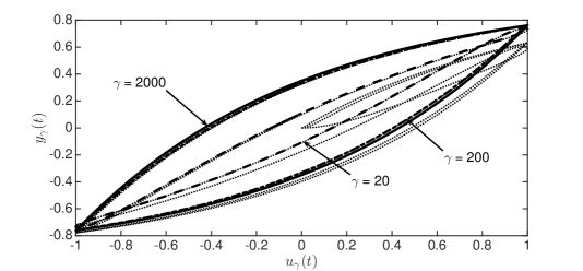
Figure 4: Output of system (18), $y_{\gamma}$ versus $u_{\gamma}$. Dotted: transient; solid: steady state for $\gamma=2000$; dashed: steady state for $\gamma=200$; dash-dotted: steady state for $\gamma=20$.

It can be seen that, as $\gamma\rightarrow\infty$, the steady-state part of the output-versus-input graph converges to a fixed closed curve. This curve is the hysteresis loop of system (18).

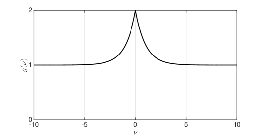
Figure 5: The macrodamping friction function $g(\nu)$ versus $\nu$.

4.2 Example 2: the hysteresis loop of the LuGre model

The aim of this section is to illustrate the concepts presented in Section 3.2.1 by means of numerical simulations.

Following [2], to approximate the Stribeck effect we set:

$$g(\nu)=F_{c}+\left(F_{s}-F_{c}\right)\mathrm{e}^{-\left|\nu/v_{s}\right|^{\beta}}\,\mbox{ for }\nu\in\mathbb{R},$$

where $F_{c}>0$ is the Coulomb friction force, $F_{s}>0$ is the stiction force, $v_{s}>0$ is the Stribeck velocity, and $\beta$ is a strictly positive constant. The function $f$ is taken to be zero. The values of the different constants are taken to be $\sigma_{0}=1$, $\sigma_{1}=1$, $F_{c}=1$, $F_{s}=2$, $v_{s}=1$, $\beta=1$, see Figure 5.

The input is the continuous $2$-periodic piecewise-linear function defined by $u(t)=t$ for $t\in[0,1]$ and $u(t)=2-t$ for $t\in[1,2]$; see Figure 6. Observe that $\psi_{u}=u$.

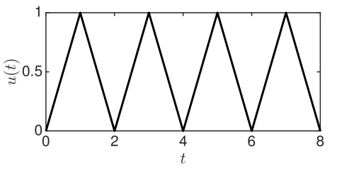
Figure 6: $u(t)$ versus $t$.

We take $x\left(0\right)=x_{0}=0$. With these values we obtain $y_{\gamma}$ by a numerical integration of Equations (5) using Matlab solver ode23s.. Also, using Equations (6)–(7) we obtain $y^{\star}_{u}$. Figure 7 provides the plots $y_{\gamma}(t)$ versus $t$ for $\gamma=1,10,100$ along with the plot $y^{\star}_{u}(t)$ versus $t$. It can be seen that as $\gamma$ increases, $y_{\gamma}$ converges to $y^{\star}_{u}$.

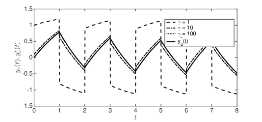
Figure 7: $y_{\gamma}(t)$ versus $t$. Dashed $\gamma=1$, dash-dotted $\gamma=10$, dotted $\gamma=100$; solid $y^{\star}_{u}(t)$ versus $t$.

The functions $y^{\star}_{u,k}$ are given by $y^{\star}_{u,k}(t)=y^{\star}_{u}(t+kT),t\in[0,T],k\in\mathbb{N}$ whilst $y_{u}^{\circ}$ is calculated from Equations (8) and (10). Figure 8 provides the plots $y^{\star}_{u,k}(t)$ versus $t$ for increasing values of $k$. It can be seen that $y^{\star}_{u,k}$ converges to $y_{u}^{\circ}$ as $k\rightarrow\infty$.

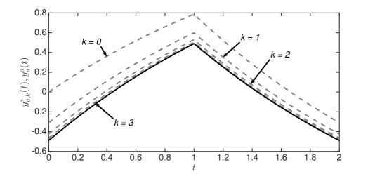
Figure 8: Convergence of the functions $y^{\star}_{u,k}$ to $y_{u}^{\circ}$. Dashed $y^{\star}_{u,k}(t)$ versus $t$ for $k=0,1,2,3$; solid $y_{u}^{\circ}(t)$ versus $t$.

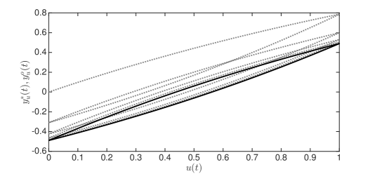
Figure 9: Convergence of the output-versus-input graph $G^{\star}_{u}$ to the hysteresis loop $G^{\circ}_{u}$. Dotted $G^{\star}_{u}$; solid $G^{\circ}_{u}$.

As in Example 1, the hysteresis loop is the output-versus-input graph obtained for very slow inputs (that is when $\gamma\rightarrow\infty$) in steady state (that is when $k\rightarrow\infty$). For a given $\gamma$, the corresponding output-versus-input graph is the set $G_{u\circ s_{\gamma}}=\big{\{}\big{(}u\circ s_{\gamma}(t),F_{\gamma}(t)\big{)},t\geq 0\big{\}}=\big{\{}\big{(}u(t),F_{\gamma}\circ s_{1/\gamma}(t)=y_{\gamma}(t)\big{)},t\geq 0\big{\}}$. Owing to Theorem 2 (a) and to [11, Lemma 9] it comes that the graphs $G_{u\circ s_{\gamma}}$ converge in a sense detailed in [11] to the graph $G^{\star}_{u}=\big{\{}\big{(}u(t),y^{\star}_{u}(t)\big{)},t\geq 0\big{\}}$ as $\gamma\rightarrow\infty$. Equations (8) and (10) provide the analytic expression of the hysteresis loop (9). Finally, Figure 9 provides the graph $G^{\star}_{u}$ along with the hysteresis loop $G^{\circ}_{u}$.

4.3 Example 3: process of convergence that leads to the hysteresis and minor loops

The aim of Sections 4.3 and 4.4 is to illustrate Theorem A by means of numerical simulations. Section 4.3 focuses on the process of convergence that leads to the hysteresis loop. Section 4.4 focuses on the variation of the minor loop with the model’s parameters.

The function $g$ that characterizes the Stribeck effect is the same as in Section 4.2. Also, the function $f$ is taken to be zero.

The input is the continuous $\rho_{4}$-periodic piecewise-linear function defined by Equation (12) where $u_{\min,1}=0$, $u_{\min,2}=0.2$, $u_{\max,1}=1$, $u_{\max,2}=1.5$, $\varrho_{1}=1$, $\varrho_{2}=1.8$, $\varrho_{3}=3.1$, $\varrho_{4}=4.6$, see Figure 10. Observe that $\psi_{u}=u$ and that the normalized variable $\varrho$ is equal to time $t$.

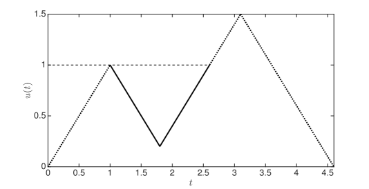
Figure 10: $u(t)$ versus $t$.

We take $x\left(0\right)=x_{0}=0$. With these values we obtain $y_{\gamma}$ by a numerical integration of Equations (5) using Matlab solver ode23s. Also, using Equations (6)–(7) we obtain $y^{\star}_{u}$. Figure 11 provides the plots $y_{\gamma}(t)$ versus $t$ for $\gamma=1,10,100$ along with the plot $y^{\star}_{u}(t)$ versus $t$. It can be seen that as $\gamma$ increases, $y_{\gamma}$ converges to $y^{\star}_{u}$.

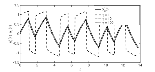
Figure 11: $y_{\gamma}(t)$ versus $t$. Dashed $\gamma=1$, dash-dotted $\gamma=10$, dotted $\gamma=100$; solid $y^{\star}_{u}(t)$ versus $t$.

The functions $y^{\star}_{u,k}$ are given by $y^{\star}_{u,k}(t)=y^{\star}_{u}(t+k\varrho_{4}),t\in[0,\varrho_{4}],k\in\mathbb{N}$ whilst $y_{u}^{\circ}$ is calculated from Equations (8) and (10). Figure 12 provides the plots $y^{\star}_{u,k}(t)$ versus $t$ for increasing values of $k$. It can be seen that $y^{\star}_{u,k}$ converges to $y_{u}^{\circ}$ as $k\rightarrow\infty$.

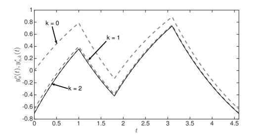
Figure 12: Convergence of the functions $y^{\star}_{u,k}$ to $y_{u}^{\circ}$. Dashed $y^{\star}_{u,k}(t)$ versus $t$ for $k=0,1,2$; solid $y_{u}^{\circ}(t)$ versus $t$.

Figure 13 provides the graphs $\big{\{}\big{(}u(t),y^{\star}_{u,k}(t)\big{)},t\in[0,\varrho_{4}]\big{\}}$ for $k=0,1,2$. It can be seen that these graphs converge to the hysteresis loop $\big{\{}\big{(}u(t),y_{u}^{\circ}(t)\big{)},t\in[0,\varrho_{4}]\big{\}}$.

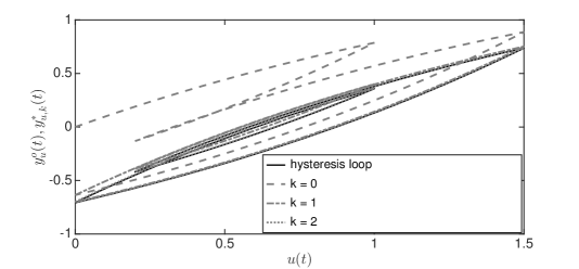
Figure 13: Convergence of the graphs $\big{\{}\big{(}u(t),y^{\star}_{u,k}(t)\big{)},t\in[0,\varrho_{4}]\big{\}}$ to the hysteresis loop $\big{\{}\big{(}u(t),y_{u}^{\circ}(t)\big{)},t\in[0,\varrho_{4}]\big{\}}$.

4.4 Example 4: Variation of the minor loop with the model’s parameters

We consider the LuGre model of Section 4.2 with the value $\sigma_{0}=6$. The input $u$ is the one given in (12) (thus a normalized one) with $u_{\min,1}=0$, $u_{\min,2}=0.5$, $u_{\max,1}=1$, $u_{\max,2}=1.5$, with its corresponding values of $\varrho_{i}=t_{i}$ for $i=1,\ldots,5$, see Figure 14.

The hysteresis loop which is given in Figure 15 is obtained using Equations (13)–(16). Observe that the shape of the minor loop depends greatly on the parameters $\sigma_{0}$, $F_{s}$, and on the relative values $u_{\min,2}-u_{\min,1}$, $u_{\max,1}-u_{\min,1}$, and $u_{\max,2}-u_{\min,1}$, see Figures 16 and 17.

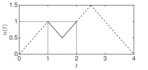
Figure 14: $u(t)$ versus $t$

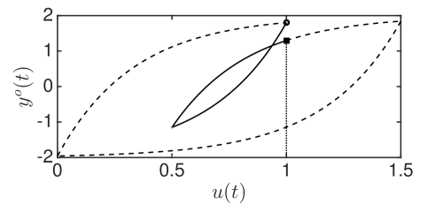
Figure 15: Hysteresis loop $G_{u}^{\circ}$. The marker open circle corresponds to the point $\big{(}u(t_{1}),y^{\circ}(t_{1})\big{)}$ whilst the marker rectangle corresponds to the point $\big{(}u(t_{5}),y^{\circ}(t_{5})\big{)}$. The minor loop is plotted in solid line.

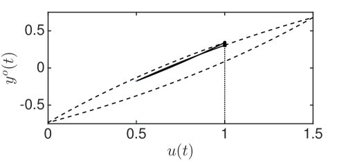
Figure 16: Hysteresis loop $G_{u}^{\circ}$ for $\sigma_{0}=1$ (minor loop in solid line).

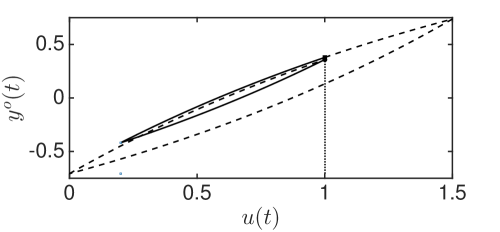
Figure 17: Hysteresis loop $G_{u}^{\circ}$ for $\sigma_{0}=1$ and $u_{\min,2}=0.2$ (minor loop in solid line).

5 Conclusions

Although the phenomenon of hysteresis has been studied since the second half of the 19th century, the behavior of minor loops as a specific issue did not emerge as a research subject until the second half of the 20th century. The present paper is framed within the increasing interest in the study of the behavior of minor loops. The originality of this work comes from being the first to provide an explicit analytic expression of the minor loops of the LuGre and the Dahl models. Our construction can be generalized to multimodal input functions giving rise to hysteresis loops with many minor loops. The obtained analytic expressions have been illustrated by means of numerical simulations.

Compliance with Ethical Standards

Conflict of Interest: The authors declare that they have no conflict of interest.

References

References

- [1] N. Aguirre-Carvajal, F. Ikhouane, J. Rodellar and R. Christenson, Parametric identification of the Dahl model for large scale MR dampers, Struct. Cont. Health Monit. 19(3) (2012) 332–347.
- [2] K. Åström, C. Canudas-de-Wit, Revisiting the LuGre friction model, IEEE Control Syst. Mag. 28(6) (2008) 101–114.
- [3] G. Bertotti, I. Mayergoyz, ed., The Science of Hysteresis, 3-volume set, Elsevier, Academic Press, Oxford, UK, 2006.
- [4] M. Brokate, J. Sprekels, Hysteresis and Phase Transitions, 121, Springer-Verlag, New York, USA, 1996.
- [5] C. Canudas de Wit, H. Olsson, K. Åström, P. Lischinsky, A new model for control of systems with friction, IEEE Trans. Autom. Control 40(3) (1995) 419–425.
- [6] P. Dahl, Solid friction damping of mechanical vibrations, AIAA J. 14(12) (1976) 1675–1682.
- [7] R-F. Fung, C-F. Han, J-L. Ha, Dynamic responses of the impact drive mechanism modeled by the distributed parameter system, Appl. Math. Model. 32(9) (2008) 1734–1743.
- [8] I. García-Baños, F. Ikhouane, A new method for the identification of the parameters of the Dahl model, J. Phys.: Conf. Series. 744(1) (2016) Article ID 012195.
- [9] C. Graczykowski, P. Pawłowski, Exact physical model of magnetorheological damper, Appl. Math. Model. 47 (2017) 400–424.
- [10] M. Hamimid, S. M. Mimoune, M. Feliachi, K. Atallah, Non centered minor hysteresis loops evaluation based on exponential parameters transforms of the modified inverse Jiles–Atherton model, Physica B, 451 (2014) 16–19.
- [11] F. Ikhouane, Characterization of hysteresis processes, Math. Control Signal Syst. 25(3) (2013) 291–310.
- [12] F. Ikhouane, A survey of the hysteretic Duhem model, Arch. Comput. Method Eng. 25(4) (2018) 965–1002.
- [13] F. Ikhouane, J. Rodellar, Systems with Hysteresis: Analysis, Identification and Control using the Bouc-Wen model, John Wiley & Sons, The Atrium, Southern Gate, Chichester, England, 2007.
- [14] K. Jankowski, M. Marszał, A. Stefański, Formulation of presliding domain non-local memory hysteretic loops based upon modified Maxwell slip model, Tribol. Lett. (2017) 65:56.
- [15] G. Leoni, A First Course in Sobolev Spaces, The American Mathematical Society, USA, 2009.
- [16] J.W. Macki, P. Nistri, P. Zecca, Mathematical models for hysteresis, SIAM Rev. 35(1) (1993) 94–123.
- [17] I. Mayergoyz, Mathematical Models of Hysteresis, Elsevier Series in Electromagnetism, Elsevier, 2003.
- [18] M. F. M. Naser, F. Ikhouane, Consistency of the Duhem model with hysteresis, Math. Probl. Eng. (2013) Article ID 586130, 16 pages.
- [19] M. F. M. Naser, F. Ikhouane, Hysteresis loop of the LuGre model, Automatica, 59 (2015) 48–53.
- [20] J. Oh, D.S. Bernstein, Semilinear Duhem model for rate-independent and rate-dependent hysteresis, IEEE Trans. Autom. Control 50(5) (2005) 631–645.
- [21] W. Rudin, Real and complex analysis, 3rd ed. McGraw-Hill, New York, 1987.
- [22] A. Visintin, Differential Models of Hysteresis, Springer-Verlag, Berlin, Heidelberg, 1994.
- [23] E.H. Yen, H.R. Van Der Vaart, On measurable functions, continuous functions and some related concepts, Am. Math. Mon. 73(9) (1966) 991–993.
- [24] H.Y. Zhao, C. Ragusa, O. de la Barriere, M. Khan, C. Appino, F. Fiorillo, Magnetic loss versus frequency in non-oriented steel sheets and its prediction: minor loops, PWM, and the limits of the analytical approach, IEEE Trans. Magn. 53(11) (2017) Article ID 2003804.