A Nonstationary Designer Space-Time Kernel

Abstract

In spatial statistics, kriging models are often designed using a stationary covariance structure; this translation-invariance produces models which have numerous favorable properties. This assumption can be limiting, though, in circumstances where the dynamics of the model have a fundamental asymmetry, such as in modeling phenomena that evolve over time from a fixed initial profile. We propose a new nonstationary kernel which is only defined over the half-line to incorporate time more naturally in the modeling process.

1 Introduction

Covariance kernels for Gaussian random fields can be defined in a number of ways—see, e.g., [16] or [9]. In spatial statistics applications in $\mathbb{R}^{d}$, kernels are often radial: the covariance between random field values at two points ${\mathbf{x}},{\mathbf{z}}\in\mathbb{R}^{d}$ is defined through a sense of distance between ${\mathbf{x}}$ and ${\mathbf{z}}$ [21].

Radial covariance kernels (sometimes referred to as radial basis functions) have numerous advantageous properties, such as computational efficiency and Bochner’s theorem of positive definiteness [7, 19]. However, they also yield stationary kriging models, which is not always ideal. Some work has been done to try to build nonstationary models from stationary kernels (see, e.g., [15] or [13]).

Another strategy to permit nonstationary models is to use nonstationary kernels, e.g., polynomial kernels [20]. Strategies such as power series kernels [23], Green’s kernels [10], and kernels derived from weighted Sobolev spaces [5] can frequently (though not necessarily) yield nonstationary kernels. Additionally, complicated (possibly nonstationary) kernels can be constructed from simpler (possibly stationary) kernels through addition or multiplication (see [2] for a thorough discussion and [14] for recent applications) or through transforms [18].

One of the benefits of designing special kernels through strategies such as weighted/generalized Sobolev spaces is to create kernels which satisfy certain properties such as smoothness, locality or boundary behavior. In this paper, we adapt a strategy for designing kernels in a bounded domain to design a kernel on the half-line. We explore the properties of this kernel as well as its viability for contributing to modeling space-time phenomena.

2 Mercer series kernels

Given a compact domain $\Omega\subseteq\mathbb{R}^{d}$, Mercer’s theorem says that all positive definite kernels (i.e., covariance kernels) $K:\Omega\times\Omega\to\mathbb{R}$ have the series representation

$$K({\mathbf{x}},{\mathbf{z}})=\sum_{n=1}^{\infty}\lambda_{n}\varphi_{n}({\mathbf{x}})\varphi_{n}({\mathbf{z}}),$$ (1)

where $\lambda_{n},\varphi_{n}$ are the eigenvalues and eigenfunctions of the integral eigenvalue problem with the associated orthonormality condition

$$\int_{\Omega}K({\mathbf{x}},{\mathbf{z}})\varphi_{n}({\mathbf{x}})\rho({\mathbf{x}})\,\textup{d}{\mathbf{x}}=\lambda_{n}\varphi_{n}({\mathbf{z}}),\quad\int_{\Omega}\varphi_{m}({\mathbf{x}})\varphi_{n}({\mathbf{x}})\rho({\mathbf{x}})\,\textup{d}{\mathbf{x}}=\delta_{m,n},$$ (2)

for a weight function $\rho:\Omega\to\mathbb{R}_{+}$ such that $\int_{\Omega}\rho({\mathbf{x}})\,\textup{d}{\mathbf{x}}=1$. If $\lambda_{n}>0$, $K$ will be positive definite.

This kernel decomposition is often used theoretically to invoke the “kernel trick” for support vector machines [19]. In [16], eigenfunctions for the popular squared exponential (Gaussian) kernel were discussed. Later, in [3] and [9, Chapter 3.9], new nonstationary kernels were designed using eigenfunctions defined through a differential equation and desired orthogonality properties, respectively.

3 A kernel defined on the half-line

In this section, we design a kernel for which $\Omega=[0,\infty)$; this will match the structure of most modeling problems in time, where there is a distinct starting time for observing data, but no distinct end. Note the use of $t$ in place of ${\mathbf{x}}$ because we will primarily apply this kernel to problems in time.

3.1 Eigenfunctions from the Laguerre polynomials

We revisit the concept from [9, Chapter 3.9], but we replace the Chebyshev with the Laguerre polynomials and their associated orthogonality condition (for $\alpha>-1$)

$$L_{n}(t)=\sum_{i=0}^{n}(-1)^{i}\genfrac{(}{)}{0.0pt}{0}{n+\alpha}{n-i}\frac{t^{i}}{i!},\quad\int_{0}^{\infty}t^{\alpha}\textup{e}^{-t}L_{m}(t)L_{n}(t)\,\textup{d}t=\frac{\Gamma(n+\alpha+1)}{\Gamma(n+1)}\delta_{m,n}.$$ (3)

Analogously to the Gaussian eigenfunctions from [8], we choose the eigenfunctions to have the form

$$\varphi_{n}(t)=\gamma_{n}\textup{e}^{-\delta t}L_{n}(t),$$

for $0<\delta<\frac{1}{2}$ and a normalization constant $\gamma_{n}$. We seek to enforce the orthogonality in (2) utilizing the Laguerre polynomial orthogonality identity in (3); this suggests the weight function

$$\rho(t)=t^{\alpha}\textup{e}^{-(1-2\delta)t}\frac{(1-2\delta)^{\alpha+1}}{\Gamma(\alpha+1)},$$

which satisfies $\int_{0}^{\infty}\rho(t)\,\textup{d}t=1$. Using this we can enforce orthonormality to identify $\gamma_{n}$,

$$\int_{0}^{\infty}\varphi_{n}(t)^{2}\rho(t)\,\textup{d}t=1\quad\Rightarrow\quad\gamma_{n}=\sqrt{\frac{\Gamma(n+1)}{\Gamma(n+\alpha+1)}\frac{\Gamma(\alpha+1)}{(1-2\delta)^{\alpha+1}}}.$$

Laguerre polynomials are a natural choice for the eigenfunctions because they are orthogonal on the domain $[0,\infty)$. This yields a kernel which is inherently defined only on $[0,\infty)$ which is a more logical choice than simply restricting a kernel defined on $\mathbb{R}$ (such as the Matérn) into $[0,\infty)$. Other functions which form an orthonormal basis over $[0,\infty)$, such as the Bessel functions $J_{k}$, could also potentially be used to create different $\varphi_{n}$.

3.2 Forming a kernel from the eigenfunctions

The Mercer series (1) requires both eigenfunctions $\varphi_{n}$ and eigenvalues $\lambda_{n}$. As was the case in [9, Chapter 3.9], we have freedom in how we choose the eigenvalues; these choices will affect the smoothness of the resulting kernel. Here, we choose the eigenvalues

$$\lambda_{n}=(1-\omega)\,\omega^{n},\qquad 0<\omega<1,$$

which satisfies the positive definite criteria that $\lambda_{n}>0$ and $\sum_{n=0}^{\infty}\lambda_{n}=1<\infty$. Because these eigenvalues decay geometrically, we expect $K(\cdot,s)\in C^{\infty}(\Omega)$ [17].

At this point, the kernel is fully specified by (1); however, it is possible to define a closed form for these specific eigenvalues, so that the infinite series need not be approximated. We can utilize the generating function of the Laguerre polynomials to write the Hardy–Hille formula [22]

$$\sum_{n=0}^{\infty}\omega^{n}\frac{\Gamma(n+1)}{\Gamma\left(1+\alpha+n\right)}\,L_{n}(t)L_{n}(s)=\frac{1}{\left(ts\omega\right)^{\frac{\alpha}{2}}(1-\omega)}\textup{e}^{-\frac{\left(t+s\right)\omega}{1-\omega}}I_{\alpha}\left(\frac{2{\sqrt{ts\omega}}}{1-\omega}\right),$$ (4)

where $I_{\alpha}$ is a modified Bessel function of the first kind [6, Chapter 10.25]. The Mercer series is

$$K(t,s)=\sum_{n=0}^{\infty}\lambda_{n}\varphi_{n}(t)\varphi_{n}(s)=(1-\omega)\frac{\Gamma(\alpha+1)}{(1-2\delta)^{\alpha+1}}\textup{e}^{-\delta(t+s)}\sum_{n=0}^{\infty}\omega^{n}\frac{\Gamma(n+1)}{\Gamma\left(1+\alpha+n\right)}L_{n}(t)L_{n}(s)$$

so substituting in (4) gives the kernel in its closed form

$$K(t,s)=\frac{\Gamma(\alpha+1)}{(1-2\delta)^{\alpha+1}}\left(ts\omega\right)^{-\alpha/2}\textup{e}^{-(t+s)\left(\delta+\frac{\omega}{1-\omega}\right)}I_{\alpha}\left({\frac{2{\sqrt{ts\omega}}}{1-\omega}}\right).$$ (5)

3.3 Computing the kernel safely

The computation of the kernel in (5) may be complicated by indeterminate forms and competing terms of exponential magnitude. The latter complication can be alleviated by computing $\exp(\log(K(t,s)))$; $\log(K(t,s))$ can be safely computed by using Stirling’s approximation [6, Chapter 5.11.1] to compute $\log(\Gamma(\alpha+1))$ and leveraging the decomposition $I_{\alpha}(u)=\textup{e}^{u}\tilde{I}_{\alpha}(u)$ where $\tilde{I}_{\alpha}(u)$ is bounded and can be computed safely [1].

We can resolve indeterminate forms by utilizing the asymptotic forms of $I_{\alpha}$,

$$I_{\alpha}(u)\sim\frac{1}{\Gamma(\alpha+1)}\left(\frac{u}{2}\right)^{\alpha}\quad\text{as}\;u\to 0,\qquad\qquad I_{\alpha}(u)\sim\frac{\textup{e}^{u}}{\sqrt{2\pi u}}\quad\text{as}\;u\to\infty,$$

from [6, Chapter 10.30.1] and [6, Chapter 10.40.1], respectively. This gives the behavior of $K(\cdot,s)$ for a fixed $s\in[0,\infty)$ as

$$K(t,s) \sim\frac{1}{(1-2\delta)^{\alpha+1}(1-\omega)}\textup{e}^{-(t+s)\left(\delta+\frac{\omega}{1-\omega}\right)}\quad\text{as}\;t\to 0,$$ (6a)

$$K(t,s) \sim\frac{\Gamma(\alpha+1)}{2(1-2\delta)^{\alpha+1}}\sqrt{\frac{1-\omega}{\pi(ts\omega)^{1/2+\alpha}}}\textup{e}^{-\left(\delta+\frac{\omega}{1-\omega}\right)(\sqrt{t}-\sqrt{s})^{2}-2\left(\delta-\frac{\sqrt{\omega}}{1+\sqrt{\omega}}\right)\sqrt{ts}}\quad\text{as}\;t\to\infty.$$ (6b)

3.4 Free parameters and their interpretations/implications

As is the case with all positive definite kernels, this new kernel has free parameters which characterize its behavior: $\alpha>-1$, $0<\delta<1/2$, and $0<\omega<1$. The interplay between these parameters is nontrivial. We state here some initial analyses which we hope lay the foundation for future work.

The behavior is easiest to analyze when the argument of $I_{\alpha}$ is large and (6b) is appropriate. This can be true for both $t\to\infty$ or for any $t$ with large enough $s$, i.e., when observed data is sufficiently far from the origin. Some insights follow below (encapsulated somewhat in Figure 1).

• The exponential term guides the long-distance behavior. Its impact varies based on the relationship between $\delta$ and $\sqrt{\omega}/(1+\sqrt{\omega})$. Regardless of the value of $\delta$, the first term in the exponential dominates the second for any fixed $s$ as $t\to\infty$. implying that the kernel always goes to 0 at $\infty$.

• Similarly, the behavior of the $ts\omega$ component depends on $\alpha$ being greater than/less than/equal to -1/2. For $\delta\neq\sqrt{\omega}/(1+\sqrt{\omega})$, the $t\to\infty$ behavior of the kernel is dominated by the exponential term and $\alpha$ plays only a scaling role.

• Setting $\alpha=-1/2$ and $\delta=\sqrt{\omega}/(1+\sqrt{\omega})$ yields a kernel which has only a $\sqrt{t}-\sqrt{s}$ contribution; this implies that $\lim_{s\to\infty}\max_{t\geq 0}K(t,s)=(1+\sqrt{\omega})/2$.

• The $\omega$ term acts as a sort of inverse length scale (or shape parameter) for the kernel. The interpretation of it as a length scale is complicated for $s$ near the origin, but more obvious as $s$ grows (for observed results far from the origin).

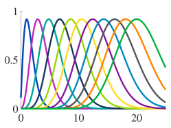
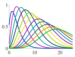
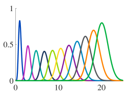
Figure 1: left: $\alpha=-.5$, $\delta=.455$, $\omega=.7$; center: $\alpha=-.7$, $\delta=.389$, $\omega=.3$; right: $\alpha=.2$, $\delta=.439$, $\omega=.95$.

4 Example: Modeling west coast temperature data

The kernel in (5) must be supplemented by components meant to model spatial phenomena. One natural mechanism for facilitating this is with a product kernel, consisting of separate time and space components (discussed in [4] and [11]). Here, we consider a tensor product between a Gaussian $K_{g}$ in space and the kernel (5), denoted here as $K_{\ell}$, in time: $K(({\mathbf{x}}\;t),\,({\mathbf{z}}\;s))=K_{g}({\mathbf{x}},{\mathbf{z}})\,K_{\ell}(t,s).$

Our example comes from the GEFS Reforecast dataset [12]; in particular, we use daily measurements for eight days of surface temperature data across the western United States with $1^{\circ}\times 1^{\circ}$ resolution. After training on seven days, we compute the Gaussian random field posterior mean on the eighth day. We use this as a prediction at each of the $28\times 29$ grid points and assess the root mean squared error (RMSE) of that prediction. This amounts to 5684 training points and 812 test points.

We explore the implications of varying the free parameters $\alpha$, $\omega$ and $\delta$ in Figure 2. To simplify the analysis, the Gaussian kernel component has a single fixed length scale in both dimensions of $.01$. We also use a fixed noise variance term (Tikhonov regularization parameter) of $10^{-8}$, primarily to avoid ill-conditioning. In principle, these quantities should be determined from the data.

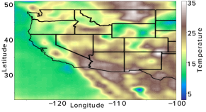
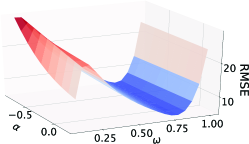
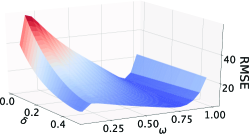
Figure 2: left: predictions made using one week’s worth of history; center: analysis of $\alpha$ and $\omega$ for $\delta=\sqrt{\omega}/(1+\sqrt{\omega})$; right: analysis of $\delta$ and $\omega$ for fixed $\alpha=0$. For $\omega$ too small, ill-conditioning plays a confounding role that requires further consideration.

Figure 2 suggests that for many values of $\omega$ the predictive power is unaffected by a wide range of $\alpha$ values. Similarly, though to a lesser extent, $\delta$ appears to have a limited and somewhat predictable effect on performance provided $\omega$ is reasonably large.

5 Future Work

This initial analysis suggests that there is an opportunity for this new kernel to help in fitting and predicting space-time data. The free parameters provide interpretable flexibility in modeling, but this comes at the cost of choosing them appropriately. Doing so will be a fundamental component of future research on the viability of this tool.

Of particular interest will be understanding how the nonstationarity and asymmetry of the kernel manifests itself in predictions at future times. Initial experimentation, including some omitted for space considerations, suggests a nontrivial interplay between $\delta$ and $\omega$; furthermore, this relationship seems to vary as observed data (and, thus, the desired region of prediction) advances from $s=0$. One future goal is to identify how existing prediction strategies, including cross-validation and maximum likelihood estimation, can be effectively adapted for this kernel.

References

- [1] D. E. Amos. Algorithm 644: A portable package for Bessel functions of a complex argument and nonnegative order. ACM Transactions on Mathematical Software (TOMS), 12(3):265–273, 1986.
- [2] A. Berlinet and C. Thomas-Agnan. Reproducing kernel Hilbert spaces in probability and statistics. Springer Science & Business Media, 2004.
- [3] R. Cavoretto, G. E. Fasshauer, and M. McCourt. An introduction to the Hilbert-Schmidt SVD using iterated Brownian bridge kernels. Numerical Algorithms, 68(2):393–422, 2015.
- [4] N. Cressie and H.-C. Huang. Classes of nonseparable, spatio-temporal stationary covariance functions. J. Am. Stat. Assoc., 94:1330–1340, 1999.
- [5] J. Dick, D. Nuyens, and F. Pillichshammer. Lattice rules for nonperiodic smooth integrands. Numerische Mathematik, 126(2):259–291, 2014.
- [6] NIST Digital Library of Mathematical Functions. http://dlmf.nist.gov/, Release 1.0.20 of 2018-09-15. F. W. J. Olver, A. B. Olde Daalhuis, D. W. Lozier, B. I. Schneider, R. F. Boisvert, C. W. Clark, B. R. Miller and B. V. Saunders, eds.
- [7] G. E. Fasshauer. Meshfree approximation methods with MATLAB, volume 6 of Interdisciplinary Mathematical Sciences. World Scientific Publishing, 2007.
- [8] G. E. Fasshauer and M. McCourt. Stable evaluation of Gaussian radial basis function interpolants. SIAM Journal on Scientific Computing, 34(2):A737–A762, 2012.
- [9] G. E. Fasshauer and M. McCourt. Kernel-Based Approximation Methods Using MATLAB, volume 19 of Interdisciplinary Mathematical Sciences. World Scientific Publishing, 2015.
- [10] G. E. Fasshauer and Q. Ye. Reproducing kernels of Sobolev spaces via a Green kernel approach with differential operators and boundary operators. Advances in Computational Mathematics, 38(4):891–921, 2013.
- [11] T. Gneiting, M. G. Genton, and P. Guttorp. Geostatistical space-time models, stationarity, separability, and full symmetry. Monographs On Statistics and Applied Probability, 107:151–175, 2006.
- [12] T. M. Hamill, G. T. Bates, J. S. Whitaker, D. R. Murray, M. Fiorino, T. J. Galarneau, Y. Zhu, and W. Lapenta. NOAA’s second-generation global medium-range ensemble reforecast dataset. Bulletin of the American Meteorological Society, 94(10):1553–1565, 2013.
- [13] Q. T. Le Gia, I. H. Sloan, and H. Wendland. Zooming from global to local: a multiscale RBF approach. Advances in Computational Mathematics, 43(3):581–606, 2017.
- [14] G. Malkomes, C. Schaff, and R. Garnett. Bayesian optimization for automated model selection. In Advances in Neural Information Processing Systems, pages 2900–2908, 2016.
- [15] R. Martinez-Cantin. Bayesian optimization with adaptive kernels for robot control. In 2017 IEEE International Conference on Robotics and Automation (ICRA), pages 3350–3356. IEEE, 2017.
- [16] C. E. Rasmussen and C. Williams. Gaussian Processes for Machine Learning. MIT Press, 2006.
- [17] J. B. Reade. Eigenvalues of positive definite kernels II. SIAM J. Math. Anal., 15(1):137–142, 1984.
- [18] Sami Remes, Markus Heinonen, and Samuel Kaski. Non-stationary spectral kernels. In Advances in Neural Information Processing Systems, pages 4642–4651, 2017.
- [19] B. Schölkopf and A. J. Smola. Learning with Kernels: Support Vector Machines, Regularization, Optimization, and Beyond. MIT Press, 2002.
- [20] J. Shawe-Taylor and N. Cristianini. Kernel Methods for Pattern Analysis. Cambridge University Press, 2004.
- [21] M. L. Stein. Interpolation of Spatial Data: Some Theory for Kriging. Springer Science & Business Media, 2012.
- [22] G. N. Watson. Notes on generating functions of polynomials: (1) Laguerre polynomials. Journal of the London Mathematical Society, 1(3):189–192, 1933.
- [23] B. Zwicknagl. Power series kernels. Constructive Approximation, 29(1):61–84, 2009.