Bounds on rare decays of $\eta$ and $\eta^{\prime}$ mesons from the neutron EDM

Abstract

We provide model-independent bounds on the rates of rare decays $\eta(\eta^{\prime})\to\pi\pi$ based on experimental limits on the neutron electric dipole moment (nEDM). Starting from phenomenological $\eta(\eta^{\prime})\pi\pi$ couplings, the nEDM arises at two loop level. The leading-order relativistic ChPT calculation with the minimal photon coupling to charged pions and a proton inside the loops leads to a finite, counter term-free result. This is an improvement upon previous estimates which used approximations in evaluating the two loop contribution and were plagued by divergences. While constraints on the $\eta(\eta^{\prime})\pi\pi$ couplings in our phenomenological approach are somewhat milder than in the picture with the QCD $\theta$-term, our calculation means that whatever the origin of these couplings, The decays $\eta(\eta^{\prime})\to 2\pi$ will remain unobservable in the near future.

I Introduction

The observed matter-antimatter asymmetry in the universe indicates that at some early stage in the evolution of the universe the $CP$-symmetry, an exact balance of the rates for processes that involve particles and antiparticles, should have been broken Sakharov (1967). However, until the discovery of $CP$-violation in $K$-meson decays, the $CP$-symmetry was believed to be an exact symmetry of the Standard Model (SM). The explanation for this $CP$-violation problem was found in the electroweak sector, involving $CP$-violating (CPV) phases of the Cabibbo-Kobayashi-Maskawa (CKM) quark-mixing matrix which allowed to accommodate the observations. Apart from meson decays, CPV interactions would also induce a static electric dipole moment for a particle with spin. Presently, there is a large number of experiments performing precise measurements of EDMs of hadrons, nuclei, atoms, and molecules Chupp et al. (2017). Furthermore, there are also data on CPV meson decays (see, e.g., Ref. Aaij et al. (2017)).

In the SM, the EDM may arise due to the CPV phases of the CKM matrix. The latest SM prediction for the nEDM Pitschmann et al. (2015) is $|d_{n}^{\rm CKM}|\approx(1-6)\times 10^{-32}\,\text{e}\cdot\text{cm}$. This range corresponds to uncertainties of low-energy constants involved in the calculations based on the heavy-baryon effective Lagrangian. Apart from the CPV in the quark mixing, the SM has no dynamical source of CP violation. Current experiments aiming at measuring the neutron and lepton EDMs are sensitive to a signal which is several orders of magnitude larger than that allowed in the SM Pendlebury et al. (2015); Tanabashi et al. (2018)

$$|d^{E}_{n}|<2.9\times 10^{-26}\,e\cdot{\rm cm}.$$ (1)

An observation of a non-zero EDM in the near future would thus point to a non-SM origin of CP violation.

In the strong-interaction sector, the nEDM is induced by the CPV $\theta$-term of quantum chromodynamics (QCD)

$$\Delta\mathcal{L}=\theta\frac{g_{s}^{2}}{32\pi^{2}}G^{a}_{\mu\nu}\tilde{G}^{a\mu\nu},$$ (2)

where $g_{s}$ is the QCD coupling constant, and $G_{\mu\nu}^{a}$ and $\tilde{G}^{a\mu\nu}=\frac{1}{2}\epsilon^{\mu\nu\alpha\beta}G^{a}_{\alpha\beta}$ are the usual stress tensor of the gluon field and its dual. The $\theta$-term preserves the renormalizability and gauge invariance of QCD, but breaks the P- and T-parity invariance. It plays an important role in QCD, e.g., for the QCD vacuum, the topological charge, and the solution of the $U(1)_{A}$ problem of the mass of the $\eta^{\prime}$ meson (see, e.g., Refs. Diakonov and Eides (1981); Witten (1979)). An explanation to the apparent smallness of the $\theta$ coupling (solution for the strong CP-violation problem) was proposed by Peccei and Quinn Peccei and Quinn (1977). They suggested $\theta$ to be a field $\theta(x)$, and decomposed it into an axial field $a(x)$ (axion) that preserves $CP$ conservation, and a small constant $\bar{\theta}$ that encodes the CPV effect. For a recent overview see, e.g., Ref. Castillo-Felisola et al. (2015).

The non-zero $\bar{\theta}$ generates a number of hadronic CPV interactions, e.g., a CPV $\pi NN$ coupling. At one loop, this coupling leads to a non-zero EDM of the nucleon. The early calculation of Ref. Crewther et al. (1979) led to a constraint on $\bar{\theta}\lesssim 6\times 10^{-10}$ based on the experimental bounds on the nEDM existing at that time. Other examples of CPV interactions among hadrons that arise in presence of the non-zero $\bar{\theta}$ are the decays $\eta(\eta^{\prime})\to 2\pi$. In the picture where the entire CP violation in hadronic interactions is due to the $\bar{\theta}$ term, the corresponding branching ratio of the order of $\sim 10^{-17}$ is unobservable. Recent advances in experimental techniques and the possibility to produce large numbers of $\eta$ and $\eta^{\prime}$ mesons at MAMI (Mainz) and Jefferson Lab (Newport News) Al Ghoul et al. (2016) has led experimentalists to look for or at least set more stringent constraints on rare decays of $\eta$ and $\eta^{\prime}$ mesons. Current experimental upper limits read Tanabashi et al. (2018); Aaij et al. (2017)

$$\rm{Br}(\eta\to\pi\pi) <\left\{\begin{array}[]{c}1.3\times 10^{-5},\;\pi^{+}\pi^{-}\\ 3.5\times 10^{-4},\;\pi^{0}\pi^{0}\end{array}\right.$$ (5)

(6)

$$\rm{Br}(\eta^{\prime}\to\pi\pi) <\left\{\begin{array}[]{c}1.8\times 10^{-5},\;\pi^{+}\pi^{-}\\ 4\times 10^{-4},\;\pi^{0}\pi^{0}\end{array}\right.$$ (9)

These bounds indicate that any signal observed within the $\sim 13-14$ orders of magnitude between the existing experimental bounds and the strong CPV expectations could be interpreted as an unambiguous signal of New Physics.

Given the experimental constraints on the nEDM it is also informative to ask how large a CPV $\eta^{(^{\prime})}\pi\pi$ interaction generated by an unspecified New Physics mechanism could be. This question was raised in Ref. Gorchtein (2008) and revisited in Ref. Gutsche et al. (2017). In those works, effective CPV $\eta^{(^{\prime})}NN$ couplings were generated from an effective CPV $\eta^{(^{\prime})}\to\pi\pi$ coupling via a pion loop. At a second step, those CPV couplings were used to generate the nEDM, again at one-loop. Because both the neutron and the $\eta$’s have no charge, the only way to couple an external photon to obtain the nEDM was magnetically. As a result, each loop is logarithmically divergent, leading to the need of counterterms which made the results less conclusive.

In this paper, we opt for a direct two-loop calculation and account for the minimal photon coupling to charged particles inside the loop. We use the leading-order ChPT Lagrangian for the coupling between pseudoscalar mesons and nucleons. CP violation is assumed to stem solely from the $\eta^{(\prime)}\pi\pi$ coupling. Anticipating the findings of our work, we obtain a resulting contribution to the nEDM which is UV-finite. We are thus able to derive very robust constraints on the CPV $\eta^{(\prime)}\to\pi\pi$ decay branching ratios from the tight experimental bounds on the nEDM,

$$\mathrm{Br}(\eta\to\pi^{+}\pi^{-})<5.3\times 10^{-17}\,,$$

$$\mathrm{Br}(\eta\to\pi^{0}\pi^{0})<2.7\times 10^{-17}\,,$$

$$\mathrm{Br}(\eta^{\prime}\to\pi^{+}\pi^{-})<5.0\times 10^{-19}\,,$$

$$\mathrm{Br}(\eta^{\prime}\to\pi^{0}\pi^{0})<2.5\times 10^{-19}\,.$$

It makes the observation of these decay channels hardly possible, independent of the particular mechanism that may lead to the generation of such an interaction. While previous calculations Gorchtein (2008); Gutsche et al. (2017) contained an uncertainty due to the divergences in chiral loops, this work represents an exact LO chiral result. As compared to the QCD $\theta$-term constraints on $\eta^{(\prime)}\to\pi\pi$ decays, the above bounds are only slightly less stringent.

The paper is organized as follows. In Sec. II we discuss the CPV couplings of the $\eta$ and $\eta^{\prime}$ mesons with two pions. In Sec. III we present the calculation of the nEDM at two loops with leading order ChPT meson-nucleon interaction, and refer details of the two-loop calculation to Appendix A. In Sec. IV we derive the upper bounds for the $\eta\to 2\pi$ and $\eta^{\prime}\to 2\pi$ decay rates.

II CPV decay constants

We begin by considering the rare CPV decays $\eta(\eta^{\prime})\to 2\pi$. For the masses and full widths of the $\eta$ and $\eta^{\prime}$ mesons we use the PDG values Tanabashi et al. (2018): $m_{\eta}=547.862\pm 0.017$ MeV, $\Gamma_{\eta}^{\text{full}}=1.31\pm 0.05$ keV and $m_{\eta^{\prime}}=957.78\pm 0.06$ MeV, $\Gamma_{\eta^{\prime}}^{\text{full}}=0.196\pm 0.009$ MeV.

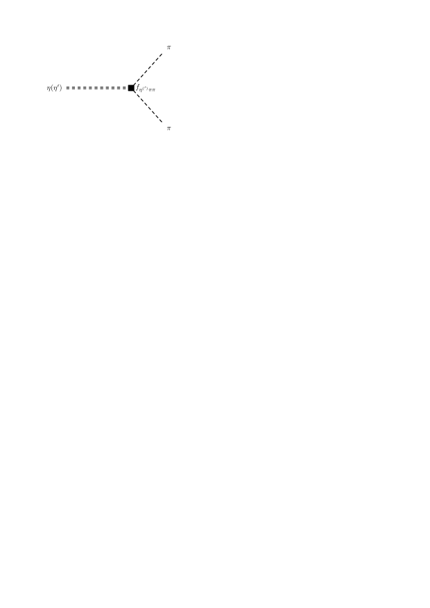
Figure 1: The $\eta(\eta^{\prime})\to\pi\pi$ decay process. The solid square represents the CPV vertex.

The effective Lagrangian that generates the P- and T-violating processes $\eta(\eta^{\prime})\to 2\pi$ (see Fig. 1) has the form

$${\cal{L}}=f_{H\pi\pi}m_{H}H\vec{\pi\,}^{2}\,,\quad H=\eta,\eta^{\prime}\,,$$ (11)

where $m_{H}$ is the mass of the $\eta(\eta^{\prime})$ meson, the pion field $\vec{\pi}$ is a isovector, $f_{H\pi\pi}$ is the corresponding coupling constant chosen to be dimensionless and defined for pions and $\eta(\eta^{\prime})$ mesons on the mass shell. The values of the $f_{\eta(\eta^{\prime})\pi\pi}$ are related to the corresponding branching ratios according to

$${\rm Br}(H\to\pi\pi)=\frac{\Gamma_{H\to\pi\pi}}{\Gamma_{H}^{full}}=n_{\Gamma}\,\frac{\sqrt{m_{H}^{2}-4m_{\pi}^{2}}}{4\pi\Gamma_{H}^{full}}f_{H\pi\pi}^{2}\,.$$ (12)

The factor $n_{\Gamma}$ is $1/2$ for the $\pi^{0}\pi^{0}$ and 1 for the $\pi^{+}\pi^{-}$ channel and reflects the Bose statistics for identical particles in the final state.

There are two possible generic mechanisms for the generation of these effective Lagrangians. The first scenario, which is fully explored in literature, is the solution to the strong $U(1)_{A}$ problem in terms of the QCD $\theta$-term that generates both the $\eta\to\pi\pi$ decay and the nucleon EDM Crewther et al. (1979); Pich and de Rafael (1991); Shifman et al. (1980). The effective $\eta^{(^{\prime})}\pi\pi$ couplings in this scenario are given by Crewther et al. (1979); Shifman et al. (1980)

$$f_{\eta\pi\pi}^{\theta} = -\frac{1}{\sqrt{3}}\,\frac{\theta\,m_{\pi}^{2}\,R}{F_{\pi}\,m_{\eta}\,(1+R)^{2}}\,,$$ (13)

$$f_{\eta^{\prime}\pi\pi}^{\theta} = -\sqrt{\frac{2}{3}}\,\frac{\theta\,m_{\pi}^{2}\,R}{F_{\pi}\,m_{\eta^{\prime}}\,(1+R)^{2}}\,,$$ (14)

where $\theta$ is the QCD vacuum angle, $R=m_{u}/m_{d}$ is the ratio of the $u$ and $d$ current quark masses, $F_{\pi}=92.4$ MeV is the pion decay constant, and $m_{\pi}=139.57$ MeV is the charged pion mass. In this scenario, the decay constant is proportional to the $\theta$-term, which is tightly constrained by the experimental bounds on the neutron EDM Harris et al. (1999); Baker et al. (2006). It is also seen that $\eta^{(^{\prime})}\pi\pi$ couplings vanish in the chiral limit $m_{\pi}\to 0$ resulting in an additional suppression. As a result, the bound for the decay constants in Eq. (11) is $(f_{\eta\pi\pi},f_{\eta^{\prime}\pi\pi})\sim(0.03\,\theta,0.05\,\theta)$. The EDM bound $\theta<6\cdot 10^{-10}$ Crewther et al. (1979); Pospelov and Ritz (1999); Balla et al. (1999) makes experimental searches for the $\eta(\eta^{\prime})$ decaying into two pions hopeless.

The second scenario corresponds to the situation where the EDM and the CPV $\eta\to\pi\pi$ vertices are generated by two distinct mechanisms, without specifying details of a particular model in which this scenario would be realized. Given the interest in addressing these decay channels experimentally at Jefferson Lab Al Ghoul et al. (2016), it is informative to inquire, how much room there is for New Physics contributions that could lead to anomalously large $\eta\pi\pi$ coupling constants. The unknown New Physics mechanism would then generate a non-zero $f_{\eta\pi\pi}$, which through pseudoscalar meson couplings to the nucleon generates the EDM at the two-loop level.

III Neutron EDM induced by CPV couplings

The electromagnetic nucleon vertex in presence of $CP$-violation is written in terms of Dirac, Pauli and electric dipole form factors $F_{E}(Q^{2}),F_{M}(Q^{2}),F_{D}(Q^{2})$, respectively,

$$\bar{u}_{N}(p_{2})\Gamma^{\mu}(p_{1},p_{2})u_{N}(p_{1})=\bar{u}_{N}(p_{2})\left[\gamma^{\mu}F_{E}(Q^{2})\right.$$

$$+\,\left.\frac{i\sigma^{\mu\nu}k_{\nu}}{2m}F_{M}(Q^{2})+\frac{i\sigma^{\mu\nu}k_{\nu}\gamma_{5}}{2m_{N}}F_{D}(Q^{2})\right]u_{N}(p_{1}).$$ (15)

Here, $Q^{2}=-k^{2}=-(p_{2}-p_{1})^{2}$, $m_{N}$ is the nucleon mass, $\gamma^{\mu}$, $\gamma_{5}$ are the Dirac matrices, and $\sigma^{\mu\nu}=\frac{i}{2}[\gamma^{\mu},\gamma^{\nu}]$. The electric dipole moment of the neutron is defined as $d^{E}_{n}=-F_{D}(0)/(2m_{N})$.

For calculating the pseudoscalar meson loops we use the non-derivative pseudoscalar (PS) couplings between mesons and nucleons. The pseudoscalar approach is obtained from the more commonly used pseudovector (PV) theory by means of a well-known chiral rotation of the nucleon fields. The two theories are equivalent (see details in Refs. Lyubovitskij et al. (2001, 2002); Lensky and Pascalutsa (2010)), and at leading order the only term in the Lagrangian involving pion and nucleon fields is

$${\cal L}_{\pi NN}^{\rm PS} = g_{\pi NN}\,\bar{N}\,i\gamma_{5}\vec{\pi}\vec{\tau}\,N\,,\quad g_{\pi NN}=\frac{g_{A}}{F_{\pi}}m_{N},$$

$${\cal L}_{\eta NN}^{\rm PS} = g_{\eta NN}\,\bar{N}\,i\gamma_{5}\eta\,N\,,$$ (16)

where $g_{A}\approx 1.275$ is the nucleon axial charge and $F_{\pi}\approx 92.4$ MeV the pion decay constant. In $SU(3)$ limits, the $\eta N$ couplings $g_{\eta^{(\prime)}NN}$ would also be related to the respective axial couplings $g_{A}^{\eta}$ and decay constants $F_{\eta}$, and similarly for $\eta^{\prime}$. However, $SU(3)$ symmetry appears to be significantly broken for these couplings and recent analyses of $\eta$ and $\eta^{\prime}$ photoproduction on nucleons suggests much smaller values Tiator et al. (2018):

$$g_{\eta NN}\approx g_{\eta^{\prime}NN}\approx 0.9\,.$$ (17)

Using the ingredients specified above, we can calculate the induced nEDM. The advantage of the pseudoscalar as compared to the pseudovector pion-nucleon theory is two-fold. Firstly, because the coupling is non-derivative the result is finite. Secondly, the number of graphs to be calculated at leading order is reduced significantly because the only way to couple the electromagnetic field to the pion field is minimally to the charged pion lines inside the loop. Unlike in the PV theory where the contact (Kroll-Ruderman) $\gamma\pi NN$ interaction term appears in the leading order chiral Lagrangian, in the pseudoscalar theory this term is generated at the level of matrix element at order $1/F_{\pi}$ and the same is true for the $\gamma\pi\pi NN$ term appeared at order $1/F_{\pi}^{2}$ Lyubovitskij et al. (2001, 2002).

The full set of two-loop Feynman diagrams to be calculated is shown in Fig. 2. Only diagrams that contribute to the nEDM are displayed. For instance, the class of diagrams that involve the contact $\pi\pi NN$ coupling gives no contribution to the nEDM and is dropped from Fig. 2. Among those diagrams that contribute there are further symmetry considerations that allow to reduce the number of independent graphs. From hermitian conjugation of matrix elements, after using replacements of nucleon momenta $p_{1}\leftrightarrow p_{2}$ and the inverse of the photon momentum $k\leftrightarrow-k$ we show result in the following relations:

$$d_{n}^{E;a}=d_{n}^{E;b}\,,\quad d_{n}^{E;c}=d_{n}^{E;d}\,,\quad d_{n}^{E;e}=d_{n}^{E;l}\,,$$

$$d_{n}^{E;f}=d_{n}^{E;k}\,,\quad d_{n}^{E;g}=d_{n}^{E;h}\,.$$ (18)

Therefore, the total contribution to the nEDM is

$$d_{n}^{E}=2\,(d_{n}^{E;a}+d_{n}^{E;c}+d_{n}^{E;e}+d_{n}^{E;f}+d_{n}^{E;g})\,.$$ (19)

The detailed calculation of the two-loop diagrams is reported in Appendix A.

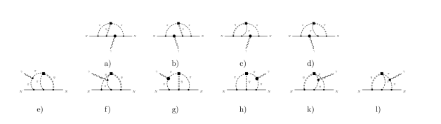
Figure 2: Diagrams describing the nEDM. The interaction with the external electromagnetic field occurs through the minimal electric coupling to charged baryon or meson fields. The solid square denotes the CPV $\eta\,\pi^{+}\pi^{-}$ vertex.

IV Results and discussion

Upon evaluating the two-loop diagrams we obtain an expression for the nEDM induced by the CPV $\eta(\eta^{\prime})\pi\pi$ couplings via meson loops and minimal coupling to the electromagnetic field,

$$d_{n}^{E} \simeq\frac{eg_{\pi NN}^{2}}{(4\pi)^{4}}\left[9.3\,\frac{g_{\eta NN}m_{\eta}}{m_{N}^{2}}f_{\eta\pi\pi}+6.4\,\frac{g_{\eta^{\prime}NN}m_{\eta}^{\prime}}{m_{N}^{2}}f_{\eta^{\prime}\pi\pi}\right]$$

$$\simeq(c_{\eta}f_{\eta\pi\pi}+c_{\eta^{\prime}}f_{\eta^{\prime}\pi\pi})\times 10^{-16}\text{e}\cdot\text{cm}\,,$$

$$c_{\eta} =6.7\,,\quad c_{\eta^{\prime}}=7.9\,.$$ (20)

The numerical difference between the two coefficients arises due to the $\eta$ and $\eta^{\prime}$ mass dependence in the loop integrals. Note that the two coefficients do not contain chiral divergences $\sim 1/m_{\pi}$ or $\sim\ln m_{\pi}$, and are evaluated by setting the pion mass to zero. For completeness, in Table 1 we present the partial contributions of the diagrams to the couplings $c_{\eta}$ and $c_{\eta^{\prime}}$.

Table 1: Contributions of diagrams to $c_{\eta}$ and $c_{\eta^{\prime}}$.

Diagram	$c_{\eta}^{a}$	$c_{\eta^{\prime}}^{a}$
a(b)	0.58	0.71
c(d)	0.56	0.67
e(l)	1.1	1.3
g(h)	1.0	1.1
f(k)	0.1	0.1
Total	6.7	7.9

Using now the current experimental bound $|d^{E}_{n}|<2.9\times 10^{-26}\,e\cdot{\rm cm}$ and assuming that the $\eta$ and $\eta^{\prime}$ couplings to two pions are independent, we deduce upper bounds on the coupling constants,

$$|f_{\eta\pi\pi}(m_{\eta}^{2})|<4.3\times 10^{-11},$$ (21)

$$|f_{\eta^{\prime}\pi\pi}(m_{\eta^{\prime}}^{2})|<3.7\times 10^{-11}\,.$$ (22)

These translate into upper bounds for the respective branching ratios,

$$\mathrm{Br}(\eta\to\pi^{+}\pi^{-})<5.3\times 10^{-17}\,,$$

$$\mathrm{Br}(\eta\to\pi^{0}\pi^{0})<2.7\times 10^{-17}\,,$$

$$\mathrm{Br}(\eta^{\prime}\to\pi^{+}\pi^{-})<5.0\times 10^{-19}\,,$$

$$\mathrm{Br}(\eta^{\prime}\to\pi^{0}\pi^{0})<2.5\times 10^{-19}\,,$$

which strongly are reduced in comparison to existing experimental limits of Eq. (6). While future and ongoing measurements of the rare decay widths of the $\eta$ and $\eta^{\prime}$ into pion pairs may improve the limits of Eq. (6), our results show that no finite signal of CP violation in these processes should be expected at the currently accessible level of precision. A similar conclusion can be made about the decays of the $\eta$ and $\eta^{\prime}$ into four pions Guo et al. (2012).

If we compare the values obtained for $f_{\eta\pi\pi}$ and $f_{\eta^{\prime}\pi\pi}$ with Eq. (14), we can deduce an upper limit for the $\bar{\theta}$ parameter in the Peccei-Quinn mechanism,

$$\bar{\theta}^{\eta}<8.4\cdot 10^{-10}\,,\quad\bar{\theta}^{\eta^{\prime}}<9.0\cdot 10^{-10}\,.$$ (24)

Here we use the ratio $R=m_{u}/m_{d}=0.556$ of the canonical set of the quark masses in ChPT Gasser and Leutwyler (1982): $m_{u}=5$ MeV, $m_{d}=9$ MeV Gasser and Leutwyler (1982) at scale 1 GeV. The limit

$$\bar{\theta}^{\eta}<8.8\cdot 10^{-10}\,,\quad\bar{\theta}^{\eta^{\prime}}<9.4\cdot 10^{-10}$$ (25)

results for the average ratio $R=m_{u}/m_{d}=0.468$ of quark masses calculated in lattice QCD at a scale of 2 GeV Tanabashi et al. (2018). Compared to the bound on $\bar{\theta}$ directly obtained from the experimental constraint on nEDM, $\bar{\theta}<6\cdot 10^{-10}$ Crewther et al. (1979); Pospelov and Ritz (1999); Balla et al. (1999), our calculation shows ( this finding is independent of the assumption that CPV $\eta,\eta^{\prime}$-decays are generated by the same mechanism as the nEDM) the very tight experimental limits on the nEDM exclude large contributions to $\eta(\eta^{\prime})\to\pi\pi$ decays beyond that captured by the Peccei-Quinn mechanism. The main difference with our calculation is that in the Peccei-Quinn mechanism the CPV $\eta(\eta^{\prime})\pi\pi$ couplings are suppressed by $m_{\pi}^{2}$ in the chiral limit. We opted to relax thus constraint but the effect of this assumption is marginal. Note that the fact that our two-loop result does not contain chiral divergences essentially means that chiral symmetry does not play a role in our scenario, consistent with the assumption that the couplings $f_{\eta\pi\pi}$ and $f_{\eta^{\prime}\pi\pi}$ may not be suppressed by the pion mass squared.

In summary, we derive new stringent upper limits on the CPV decays $\eta\to\pi\pi$ and $\eta^{\prime}\to\pi\pi$. The presence of an effective CPV $\eta^{(^{\prime})}\pi\pi$ interaction in the Lagrangian leads to an induced nEDM at two loop. We explicitly evaluated a full set of two-loop level of Feynman diagrams arising at leading chiral order in relativistic ChPT with the pseudoscalar pion-nucleon coupling, which are free from divergences. The tight experimental bounds on the nEDM lead to upper limits for $|f_{\eta\pi\pi}|$ and $|f_{\eta^{\prime}\pi\pi}|$ which thus cannot exceed few parts times $10^{-11}$. These translate into upper limits for the branching ratios $\mathrm{Br}(\eta\to\pi\pi)$ and $\mathrm{Br}(\eta^{\prime}\to\pi\pi)$, which are of order $10^{-17}$ or even smaller.

In the future, we plan to continue our study of rare decays of $\eta$ and $\eta^{\prime}$ mesons. In particular, in our scenario only the decays into charged pions are strictly speaking constrained. The bound on the neutral decays is obtained by isospin symmetry. In presence of isospin symmetry breaking the couplings $f_{\eta\pi^{+}\pi^{-}}$ and $f_{\eta\to\pi^{0}\pi^{0}}$ will be unrelated. In this case, with all neutral particles in the loops the nEDM can be generated via a magnetic coupling of the photon to the neutron.

Appendix A Calculation technique of the two-loop integrals

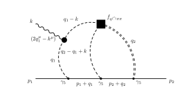
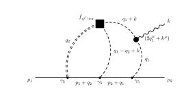
Figure 3: Diagrams e) and l) from Fig. 2. The double dashed lines correspond to the $\eta^{(\prime)}$ mesons, the dashed lines to pions and the solid lines to baryon propagators. The CPV $\eta^{(\prime)}\pi\pi$ transition is denoted by the black box.

Here we discuss the calculational technique of the two-loop integrals occuring in the evaluation of the nEDM (see diagrams in Fig. 2). Analytic manipulation of the integrals is performed using the package FORM Vermaseren (2000). For convenience we evaluate the two-loop integrals in $d$-dimensions and finally put $d=4$.

We demonstrate all steps of the calculations for the diagrams of Fig. 2e and 2l, which are shown in more detail in Fig. 3. In particular, the matrix element generated by the diagram in Fig. 2e is

$$M_{2e}(p_{1},p_{2})=\epsilon_{\mu}(q)\bar{u}_{N}(p_{2})\Lambda_{2e}^{\mu}(p_{1},p_{2})u_{N}(p_{1})\,,$$

$$\Lambda_{2e}^{\mu}(p_{1},p_{2})=g_{\rm eff}\,\int\frac{d^{d}q_{1}}{(2\pi)^{d}i}\int\frac{d^{d}q_{2}}{(2\pi)^{d}i}\,\frac{2q_{1}^{\mu}\,i\gamma^{5}(m_{N}+\not\!p_{2}+\not\!q_{2})i\gamma^{5}(m_{N}+\not\!p_{1}+\not\!q_{1})i\gamma^{5}}{D_{N}(p_{1}+q_{1})\,D_{N}(p_{2}+q_{2})\,D_{\eta^{(^{\prime})}}(q_{2})\,D_{\pi}(q_{1})\,D_{\pi}(q_{1}-k)\,D_{\pi}(q_{2}-q_{1}+k)}\,,$$ (26)

where $u_{N}(p_{1})$ and $\bar{u}_{N}(p_{2})$ are the nucleon spinors in the initial and final state, respectively; $\epsilon_{\mu}(q)$ is the polarization vector of the photon field; $D_{H}(k)=m_{H}^{2}-k^{2}$ are the scalar denominators of virtual particles $H=N,\pi,\eta^{(^{\prime})}$. Here $g_{\rm eff}$ is the effective coupling

$$g_{\rm eff}=4eg_{\pi NN}^{2}g_{\eta^{(^{\prime})}NN}f_{\eta^{(^{\prime})}\pi\pi}m_{\eta^{(^{\prime})}}\,.$$ (27)

Using the equation of motion for the nucleon spinors the numerator is reduced to $2i\gamma^{5}q_{1}^{\mu}\not\!q_{2}\not\!q_{1}$. For the string of denominators $D_{H}$ we apply the Feynman parametrization:

$$\frac{1}{D_{1}\cdots D_{6}}=\Gamma(6)\,\int\limits_{0}^{1}d\alpha_{1}\cdots\int\limits_{0}^{1}d\alpha_{6}\,\frac{\delta\Big{(}1-\sum\limits_{i=1}^{6}\alpha_{i}\Big{)}}{\Big{(}\sum\limits_{i=1}^{6}\alpha_{i}D_{i}\Big{)}^{6}}\,.$$ (28)

Then $\Lambda_{2e}^{\mu}(p_{1},p_{2})$ takes the form

$$\Lambda_{2e}^{\mu}(p_{1},p_{2}) = 2i\gamma^{5}\gamma^{\alpha}\gamma^{\beta}\,T_{2e}^{\mu\alpha\beta}(p_{1},p_{2})\,,$$

$$T_{2e}^{\mu\alpha\beta}(p_{1},p_{2}) = \Gamma(6)\int\frac{d^{d}q_{1}}{(2\pi)^{d}i}\int\frac{d^{d}q_{2}}{(2\pi)^{d}i}\,k_{1}^{\mu}\,k_{2}^{\alpha}\,k_{1}^{\beta}\,\int\limits_{0}^{1}d\alpha_{1}\cdots\int\limits_{0}^{1}d\alpha_{6}\,\delta\Big{(}1-\sum\limits_{i=1}^{6}\alpha_{i}\Big{)}\,\frac{1}{(\Delta-qAq-2Bq)^{6}}\,.$$ (29)

Here

$$qAq=\sum\limits_{i,j=1}^{2}\,q_{i}\,A_{ij}\,q_{j}\,,\quad Bq=B_{1}q_{1}+B_{2}q_{2}\,,$$ (30)

where $A_{ij}$ is the $2\times 2$ matrix

$$A_{ij} = \left(\begin{array}[]{cc}\alpha_{1456}&-\alpha_{6}\\ -\alpha_{6}&\alpha_{236}\\ \end{array}\right)\,,\quad\alpha_{i_{1}\cdots i_{k}}=\alpha_{i_{1}}+\ldots+\alpha_{i_{k}}\,,$$ (33)

and

$$B_{1}=p_{1}\alpha_{1}-k\alpha_{56}\,,\quad B_{2}\,=\,p_{2}\alpha_{2}+k\alpha_{6}\,,\quad\Delta=M_{\eta^{(^{\prime})}}^{2}\alpha_{3}+M_{\pi}^{2}\alpha_{456}\,.$$ (34)

Next, each virtual momentum in the numerator of $T_{2e}^{\mu\alpha\beta}(p_{1},p_{2})$ can be replaced by the corresponding partial derivative of the two-loop integral with respect to $B_{1}^{\alpha}$ or $B_{2}^{\alpha}$ using the substitution

$$\frac{q_{i}^{\mu}}{(\Delta-qAq-2Bq)^{n}}=\frac{1}{2(n-1)}\,\frac{\partial}{\partial B_{i}^{\mu}}\frac{1}{(\Delta-qAq-2Bq)^{n-1}}\,.$$ (35)

In our case we have

$$T_{2e}^{\mu\alpha\beta}(p_{1},p_{2}) = \frac{\Gamma(3)}{2^{3}}\,\frac{\partial^{3}}{\partial B^{\mu}_{1}\partial B^{\beta}_{1}\partial B^{\alpha}_{2}}\,\int\frac{d^{d}q_{1}}{(2\pi)^{d}i}\int\frac{d^{d}q_{2}}{(2\pi)^{d}i}\int\limits_{0}^{1}d\alpha_{1}\cdots\int\limits_{0}^{1}d\alpha_{6}\,\delta\Big{(}1-\sum\limits_{i=1}^{6}\alpha_{i}\Big{)}\,\frac{1}{(\Delta-qAq-2Bq)^{3}}$$ (36)

$$= \frac{1}{({\rm det}A)^{2}}\,\frac{\Gamma(3-d)}{2^{3}(4\pi)^{d}}\frac{\partial^{3}}{\partial B^{\mu}_{1}\partial B^{\beta}_{1}\partial B^{\alpha}_{2}}\Big{(}\Delta+BA^{-1}B\Big{)}^{d-3}\,,$$

where ${\rm det}A$ and $A^{-1}$ are the determinant and inverse matrix of $A$, respectively. Note, at $q^{2}=0$ the term $BA^{-1}B$ is equal to

$$BA^{-1}B=m_{N}^{2}\Big{(}A_{11}^{-1}\alpha_{1}^{2}+A_{22}^{-1}\alpha_{2}^{2}+2A_{12}^{-1}\alpha_{1}\alpha_{2}\Big{)}\,.$$ (37)

Taking the derivatives in Eq. (36) we get

$$\frac{\Gamma(3-d)}{2^{3}}\frac{\partial^{3}}{\partial B^{\mu}_{1}\partial B^{\beta}_{1}\partial B^{\alpha}_{2}}\Big{(}\Delta+BA^{-1}B\Big{)}^{d-3} = \frac{\Gamma(5-d)}{2}\,(\Delta+BA^{-1}B)^{d-5}\,\biggl{[}g^{\alpha\beta}L_{1}^{\mu}A_{12}^{-1}\,+\,g^{\mu\alpha}L_{1}^{\beta}A_{12}^{-1}\,+\,g^{\mu\beta}L_{2}^{\alpha}A_{11}^{-1}\biggr{]}$$ (38)

$$- \Gamma(6-d)\,(\Delta+BA^{-1}B)^{d-6}\,L_{1}^{\mu}\,L_{1}^{\beta}\,L_{2}^{\alpha}\,,$$

where $L_{1}=B_{1}A_{11}^{-1}+B_{2}A_{12}^{-1}$ and $L_{2}=B_{1}A_{12}^{-1}+B_{2}A_{22}^{-1}$.

After a straigthforward calculation we keep terms proportional to the Dirac structure $i(p_{1}+p_{2})^{\mu}\gamma^{5}$, which due to Gordon identity

$$i(p_{1}+p_{2})^{\mu}\bar{u}_{N}(p_{2})\gamma^{5}u_{N}(p_{1})=\bar{u}_{N}(p_{2})\sigma^{\mu\nu}k_{\nu}\gamma^{5}u_{N}(p_{1})\,,$$ (39)

corresponds to the EDM Dirac structure in Eq. (15). The contribution of the diagram Fig. 2e to the nEDM is

$$d_{n}^{E;e} = \frac{g_{\rm eff}}{(4\pi)^{4}}\,\int\limits_{0}^{1}d\alpha_{1}\cdots\int\limits_{0}^{1}d\alpha_{6}\,\frac{\delta\Big{(}1-\sum\limits_{i=1}^{6}\alpha_{i}\Big{)}}{({\rm det}A)^{2}\,(\Delta+BA^{-1}B)}\,\biggl{[}(-A_{12}^{-1})^{2}(3\alpha_{2}+\alpha_{6})+A_{11}^{-1}A_{22}^{-1}\alpha_{6}-3A_{11}^{-1}A_{12}^{-1}\alpha_{1}$$ (40)

$$+ \frac{m_{N}^{2}}{\Delta+BA^{-1}B}\biggl{(}(A_{12}^{-1})^{3}\alpha_{2}(3\alpha_{1}\alpha_{2}+2\alpha_{1}\alpha_{6}+2\alpha_{2}\alpha_{56})+(A_{12}^{-1})^{2}A_{22}^{-1}\alpha_{2}^{3}+2(A_{12}^{-1})^{2}A_{11}^{-1}\alpha_{1}(\alpha_{2}\alpha_{56}+\alpha_{1}\alpha_{6}+2\alpha_{1}\alpha_{2})$$

$$+ (A_{11}^{-1})^{2}A_{12}^{-1}\alpha_{1}^{3}+(A_{11}^{-1})^{2}A_{22}^{-1}\alpha_{1}(\alpha_{1}\alpha_{2}+2\alpha_{1}\alpha_{6}+2\alpha_{2}\alpha_{56})-2A_{11}^{-1}A_{12}^{-1}A_{22}^{-1}\alpha_{2}(\alpha_{1}\alpha_{6}+\alpha_{2}\alpha_{56})\biggr{)}\biggr{]}\,.$$

Using our method we can evaluate the contribution of the other diagrams to the nEDM. We only present the final results in terms of integrals over Feynman parameters and specify the forms of matrix $A$, vectors $B_{1}$ and $B_{2}$, and the term $\Delta$.

The contribution of diagrams 2g(h) is given by the expression for diagram 2e(l) with only one change. The term $\Delta$ must be redefined as

$$\Delta=m_{\pi}^{2}\alpha_{345}+m_{\eta^{(^{\prime})}}^{2}\alpha_{6}\,.$$ (41)

Diagrams 2f(k) give the following contribution

$$d_{n}^{E;f} = \frac{4g_{\rm eff}}{(4\pi)^{4}}\,\int\limits_{0}^{1}d\alpha_{1}\cdots\int\limits_{0}^{1}d\alpha_{6}\,\frac{\delta\Big{(}1-\sum\limits_{i=1}^{6}\alpha_{i}\Big{)}}{({\rm det}A)^{2}\,(\Delta+BA^{-1}B)}\,\biggl{[}(-A_{12}^{-1})^{2}(\alpha_{1}-\alpha_{2})$$ (42)

$$+ 3A_{11}^{-1}A_{12}^{-1}\alpha_{1}-3A_{22}^{-1}A_{12}^{-1}\alpha_{2}+\frac{m_{N}^{2}}{\Delta+BA^{-1}B}\biggl{(}-(A_{12}^{-1})^{3}(\alpha_{1}-\alpha_{2})(2\alpha_{6}\alpha_{12}-3\alpha_{1}\alpha_{2})$$

$$- (A_{12}^{-1})^{2}A_{22}^{-1}\alpha_{2}(2\alpha_{6}\alpha_{12}+\alpha_{2}(\alpha_{2}-4\alpha_{1}))+(A_{12}^{-1})^{2}A_{11}^{-1}\alpha_{1}(2\alpha_{6}\alpha_{12}+\alpha_{1}(\alpha_{1}-4\alpha_{2}))$$

$$- (A_{11}^{-1})^{2}A_{12}^{-1}\alpha_{1}^{3}-(A_{11}^{-1})^{2}A_{22}^{-1}\alpha_{1}(2\alpha_{6}\alpha_{12}-\alpha_{1}\alpha_{2})+(A_{22}^{-1})^{2}A_{11}^{-1}\alpha_{2}(2\alpha_{6}\alpha_{12}-\alpha_{1}\alpha_{2})$$

$$+ (A_{22}^{-1})^{2}A_{12}^{-1}\alpha_{2}^{3}+2A_{11}^{-1}A_{12}^{-1}A_{22}^{-1}\alpha_{6}(\alpha_{1}^{2}-\alpha_{2}^{2})\biggr{)}\biggr{]}$$

Diagrams 2a(b) and 2c(d) result in the expresion

$$d_{n}^{E;a(c)} = \frac{6g_{\rm eff}}{(4\pi)^{4}}\,\int\limits_{0}^{1}d\alpha_{1}\cdots\int\limits_{0}^{1}d\alpha_{6}\,\frac{\delta\Big{(}1-\sum\limits_{i=1}^{6}\alpha_{i}\Big{)}}{({\rm det}A)^{2}\,(\Delta_{a(c)}+BA^{-1}B)}\,\biggl{[}2A_{12}^{-1}-6(A_{12}^{-1})^{2}\alpha_{2}-6A_{11}^{-1}A_{12}^{-1}\alpha_{1}$$ (43)

$$+ \frac{m_{N}^{2}}{\Delta_{a(c)}+BA^{-1}B}\biggl{(}-4(A_{12}^{-1})^{2}\alpha_{2}\alpha_{14}-4A_{11}^{-1}A_{12}^{-1}\alpha_{1}\alpha_{14}-4A_{11}^{-1}A_{22}^{-1}\alpha_{1}\alpha_{2}$$

$$- 4A_{12}^{-1}A_{22}^{-1}\alpha_{2}^{2}+2(A_{12}^{-1})^{3}\alpha_{2}^{2}(2\alpha_{4}+\alpha_{1})+2(A_{12}^{-1})^{2}A_{11}^{-1}\alpha_{2}\alpha_{14}^{2}+2(A_{12}^{-1})^{2}A_{22}^{-1}\alpha_{2}^{3}$$

$$+ 2(A_{11}^{-1})^{2}A_{12}^{-1}\alpha_{1}\alpha_{14}^{2}+2(A_{11}^{-1})^{2}A_{22}^{-1}\alpha_{2}(\alpha_{1}^{2}-\alpha_{4}^{2})+4A_{11}^{-1}A_{12}^{-1}A_{22}^{-1}\alpha_{1}\alpha_{2}^{2}\biggr{)}\biggr{]}$$

Here matrix $A$ is the same as for diagram 2e(l), the vectors $B_{i}$ are $B_{1}=p_{1}\alpha_{1}+p_{2}\alpha_{4}$ and $B_{2}=p_{1}\alpha_{2}$. The $\Delta$ terms are specified as:

$$\Delta_{a}=m_{\pi}^{2}\alpha_{35}+m_{\eta^{(^{\prime})}}^{2}\alpha_{6}\,,\quad\Delta_{c}=m_{\pi}^{2}\alpha_{56}+m_{\eta^{(^{\prime})}}^{2}\alpha_{3}\,.$$ (44)

One can see that the contributions of diagrams Fig.2a(b) and 2c(d) are degenerate in the limit $M_{\eta^{(^{\prime})}}=M_{\pi}$. The numerical values for these two types of diagrams at physical values of $\pi$ and $\eta^{(^{\prime})}$ masses are also close to each other.

After restoring the omitted isospin factors and couplings, we obtain the total contribution to the nEDM:

$$d_{N}^{E}= 2(d_{N}^{E;a}+d_{N}^{E;c}+d_{N}^{E;f}+d_{N}^{E;g}+d_{N}^{E;e})$$ (45)