Two-photon decay of P-wave positronium: a tutorial

Abstract

A detailed exposition of two-photon decays of P-wave positronium is given to fill an existing gap in the pedagogical literature. Annihilation decay rates of P-wave positronium are negligible compared to the rates of radiative electric dipole transitions to the ground state. This circumstance makes such decays experimentally inaccessible. However the situation is different for quarkonium and the experimental and theoretical research of two-photon and two-gluon decays of P-wave quarkonia is a still flourishing field.

I Introduction

Two-photon decay rates of positronium in the P-state were calculated long ago 1 ; 2 . A well-known textbook in quantum field theory 3 offers this problem as an exercise after presenting a basic tenets and calculation tools of this theory.

Being indeed an excellent exercise in quantum field theory, however we are afraid that most students will find it too complicated. Even if they can find the original papers about this problem 1 ; 2 , more modern presentation in 4 , or its quarkonium counterpart in 5 , this will not help much, we think.

This feeling is strengthened by the observation that in the unofficial solutions manual 6 of the textbook 3 , the decay rates of P-wave positronium are calculated incorrectly.

A detailed derivation of the two-photon amplitudes of various quarkonium states can be found in 7 . Although very useful, this paper uses the Jacob-Wick helicity formalism 8 , not covered in any detail in 3 (however this formalism is briefly considered in older QFT textbook 9 ), and therefore can seem somewhat esoteric for novices in quantum field theory.

In this paper we attempt to fill this seeming gap in pedagogical literature and provide a detailed calculation of the two-photon decay rates of P-wave positronium along general style of the first five chapters of 3 .

The decay width of S-wave positronium in non-relativistic approximation can be obtained by elementary means 9A . Namely, the probability of electron-positron annihilation in S-wave positronium per unit time is

$$\Gamma=\rho v\sigma,$$ (1)

where $v$ is electron-positron relative velocity, $\rho=|\psi(0)|^{2}$ gives a probability that the electron and positron meet each other in the positronium, and $\sigma$ is their annihilation cross-section when they meet. The later can be related to the annihilation cross-section of the free electron-positron pair as follows. We must multiply the free cross-section by four, because it was averaged over the four possible spin-states of the incident electron and positron. Besides we must take into account the selection rules that only spin-singlet S-wave positronium can decay into two-photons, and only spin-triplet positronium can decay into three-photons. This selection rule can be enforced by taking $v\to 0$ limit which in the free cross-section leaves only s-wave contribution. Finally we must average over positronium polarization states which brings $1/(2J+1)$ factor in the formula. In this way we get the Pirenne-Wheeler formula 32 :

$$\Gamma(Ps\to n\gamma)=\frac{1}{2J+1}\,|\psi(0)|^{2}\,\lim_{v\to 0}\left[4v\sigma(e^{+}e^{-}\to n\gamma)\right].$$ (2)

In the case of P-wave positronium the wave-function at the origin vanishes and the decay amplitude becomes proportional to the spatial derivatives of the wave function at the origin. Correspondingly we need the free annihilation cross-section beyond the $v\to 0$ limit and things become much more complicated. As a result there is no Pirenne-Wheeler like simple way to get annihilation cross-section of P-wave positronium. The only thing which we can predict from the beginning is that in this case the annihilation rate will be suppressed compared to the S-wave positronium annihilation rate by a factor $(|\vec{p}|/m)^{2}\sim\beta^{2}$ since this is a relative magnitude of the leading term in an expansion for small momenta 9A .

For light quarks the suppression goes away and the non-relativistic approximation breaks down completely. Even for heavy quarkonia, such as charmonium, where $\beta^{2}\sim 0.3$, and bottonium, where $\beta^{2}\sim 0.1$, the relativistic corrections are important and these corrections were studied in the frameworks of the Bethe-Salpeter equation 10A ; 10B , two-body Dirac equation 10C , covariant light-front approach 10D , sophisticated quarkonium potential model 10E , using an effective Lagrangian and QCD sum rules 10F , lattice QCD 10G , non-relativistic QCD (NRQCD) 10H , to name a few. Regarding experimental situation, see, for example, 10I ; 10J .

We hope that a detailed understanding of a more simple positronium case will help students to navigate the vast literature devoted to the two-photon and two-gluon decays of quarkonia.

II Positronium state vector

A correct framework for relativistic bound state problem is provided by the Bethe-Salpeter equation 10 ; 11 (for pedagogical discussions of this equation see 9 ; 12 ). Fortunately, for weakly bound non-relativistic systems, like positronium, this notoriously difficult formalism simplifies considerably. It was shown 13 ; 14 that the relativistic two-fermion Bethe-Salpeter equation for such systems allows a systematic perturbation theory and the corresponding lowest-order exactly solvable approximation essentially coincides to the Schrödinger equation for a single effective particle.

At the lowest-order in fine structure constant $\alpha$, and in its rest frame, the positronium state vector can be approximated by the quantum state

$$|^{2S+1}L_{J};M>=\sqrt{2M_{Ps}}\int\frac{d\vec{p}}{(2\pi)^{3}}\sum_{S_{z}=-S}^{S}\left[\begin{array}[]{ccc}l&S&J\\ M-S_{z}&S_{z}&M\end{array}\right]\tilde{\psi}_{lm}(\vec{p})|S,S_{z}>,$$ (3)

where $m=M-S_{z}$, $\tilde{\psi}_{lm}(\vec{p})=\int e^{-i\vec{p}\cdot\vec{x}}\psi_{lm}(\vec{x})\,d\vec{x}$ is the momentum space Schrödinger wave function of positronium (the principal quantum number is not indicated) giving the probability amplitude of finding the electron and positron with relative momentum $\vec{p}$ in the positronium, $M_{Ps}\approx 2m$ is the positronium mass ($m$ being the electron mass, not to be confused with the magnetic quantum number $m$ in $\tilde{\psi}_{lm}$) and the $\sqrt{2M_{Ps}}$ factor ensures a proper normalization of the positronium state vector consistent to the normalization of one-particle states adopted in 3 . The Clebsch-Gordan coefficients $\left[\begin{array}[]{ccc}l&S&J\\ m&S_{z}&M\end{array}\right]$ (a square bracket notation of 15 is used for these coefficients) couple the angular momentum eigenstates $\tilde{\psi}_{lm}(\vec{p})$ with the total spin eigenstates $|S,S_{z}>$ to form the total momentum eigenstates $|^{2S+1}L_{J};M>$ . The total spin eigenstates by themselves are the result of quantum addition of electron and positron spins:

$$|S,S_{z}>=\left[\begin{array}[]{ccc}\frac{1}{2}&\frac{1}{2}&S\\ s&S_{z}-s&S_{z}\end{array}\right]a^{+}(s,\vec{p})b^{+}(S_{z}-s,-\vec{p})|0>.$$ (4)

Here $a^{+}(s,\vec{p})$ is the creation operator of electron with spin-projection $s$ and momentum $\vec{p}$, while $b^{+}(S_{z}-s,-\vec{p})$ is the creation operator of positron with spin-projection $S_{z}-s$ and momentum $-\vec{p}$.

Note that, since particle number is not conserved in relativistic quantum field theory, in general positronium state vector may contain contributions from Fock states that have particles other than “valence” electron and positron, as in (3). However, in positronium, thanks to its non-relativistic nature, such admixtures are very small. For example, the the probability of finding relativistic relative momenta, $p\sim m$ or higher, in positronium is only $O(\alpha^{5})\sim 10^{-11}$ 15A .

We use standard spectroscopic notation in (3). In particular, $L$ refers to the orbital angular momentum quantum number $l$ written as $S,P,D,F,\ldots$ for $l=0,1,2,3,\ldots$

Electron and positron spins can combine to give either a total spin zero singlet state or a total spin one triplet states. The corresponding non-zero Clebsch-Gordan coefficients are 16

$$\left[\begin{array}[]{ccc}1/2&\;\;1/2&0\\ 1/2&-1/2&0\end{array}\right]=-\left[\begin{array}[]{ccc}\;\;1/2&1/2&0\\ -1/2&1/2&0\end{array}\right]=\frac{1}{\sqrt{2}},\;\;\left[\begin{array}[]{ccc}1/2&1/2&1\\ 1/2&1/2&1\end{array}\right]=1,$$ (11)

$$\left[\begin{array}[]{ccc}1/2&\;\;1/2&1\\ 1/2&-1/2&0\end{array}\right]=\left[\begin{array}[]{ccc}\;\;1/2&1/2&1\\ -1/2&1/2&0\end{array}\right]=\frac{1}{\sqrt{2}},\;\;\left[\begin{array}[]{ccc}\;\;1/2&\;\;1/2&\;\;1\\ -1/2&-1/2&-1\end{array}\right]=1.$$ (18)

Using them, we easily get $S$-wave positronium state vectors

$$|^{1}S_{0};0>=2\sqrt{m}\int\frac{d\vec{p}}{(2\pi)^{3}}\,\tilde{\psi}_{00}(\vec{p})\,\frac{1}{\sqrt{2}}\left[a^{+}\left(\frac{1}{2},\vec{p}\right)\,b^{+}\left(-\frac{1}{2},-\vec{p}\right)-a^{+}\left(-\frac{1}{2},\vec{p}\right)\,b^{+}\left(\frac{1}{2},-\vec{p}\right)\right]|0>,$$

$$|^{3}S_{1};0>=2\sqrt{m}\int\frac{d\vec{p}}{(2\pi)^{3}}\,\tilde{\psi}_{00}(\vec{p})\,\frac{1}{\sqrt{2}}\left[a^{+}\left(\frac{1}{2},\vec{p}\right)\,b^{+}\left(-\frac{1}{2},-\vec{p}\right)+a^{+}\left(-\frac{1}{2},\vec{p}\right)\,b^{+}\left(\frac{1}{2},-\vec{p}\right)\right]|0>,$$

$$|^{3}S_{1};1>=2\sqrt{m}\int\frac{d\vec{p}}{(2\pi)^{3}}\,\tilde{\psi}_{00}(\vec{p})\,a^{+}\left(\frac{1}{2},\vec{p}\right)\,b^{+}\left(\frac{1}{2},-\vec{p}\right)|0>,$$

$$|^{3}S_{1};-1>=2\sqrt{m}\int\frac{d\vec{p}}{(2\pi)^{3}}\,\tilde{\psi}_{00}(\vec{p})\,a^{+}\left(-\frac{1}{2},\vec{p}\right)\,b^{+}\left(-\frac{1}{2},-\vec{p}\right)|0>$$ (19)

Slightly abusing a notation (by using $s,s^{\prime}$ as matrix indexes) and changing the overall signs of some state vectors then necessary (in quantum theory state vectors are defined up to a phase), we can express (19) state vectors in a more compact way:

$$|^{2S+1}S_{J};M>=2\sqrt{m}\int\frac{d\vec{p}}{(2\pi)^{3}}\,\tilde{\psi}_{00}(\vec{p})\,\sum_{s\,s^{\prime}}a^{+}(s,\vec{p})[A^{(JM)}(-i\sigma_{2})]_{s\,s^{\prime}}b^{+}(s^{\prime},-\vec{p}))|0>,$$ (20)

where $A^{(JM)}$ matrices are expressed through the Pauli matrices and the triplet state polarization vectors

$$\vec{n}_{1}=\frac{1}{\sqrt{2}}\,(1,i,0),\;\;\vec{n}_{-1}=\frac{1}{\sqrt{2}}\,(1,-i,0),\;\;\vec{n}_{0}=(0,0,1),$$ (21)

in the following way

$$A^{(00)}=\frac{1}{\sqrt{2}},\;\;\;A^{(1M)}=\frac{1}{\sqrt{2}}\,\vec{n}_{M}\cdot\vec{\sigma}.$$ (22)

To deal with $P$-wave positronium states, it is convenient instead of $\tilde{\psi}_{1m}(\vec{p})$ eigenstates of the third component of the angular momentum, to introduce Cartesian states

$$\tilde{\psi}^{1}(\vec{p})=\frac{1}{\sqrt{2}}\left(\tilde{\psi}_{1,-1}(\vec{p})-\tilde{\psi}_{1,1}(\vec{p})\right),\;\;\;\tilde{\psi}^{2}(\vec{p})=\frac{i}{\sqrt{2}}\left(\tilde{\psi}_{1,-1}(\vec{p})+\tilde{\psi}_{1,1}(\vec{p})\right),\;\;\;\tilde{\psi}^{3}(\vec{p})=\tilde{\psi}_{1,0}(\vec{p}).$$ (23)

We also will need the following non-zero $1\otimes 1$ Clebsch-Gordan coefficients 16 :

$$\left[\begin{array}[]{ccc}1&1&1\\ 1&0&1\end{array}\right]=-\left[\begin{array}[]{ccc}1&1&1\\ 0&1&1\end{array}\right]=\left[\begin{array}[]{ccc}1&\;\;1&1\\ 1&-1&0\end{array}\right]=-\left[\begin{array}[]{ccc}\;\;1&1&1\\ -1&1&0\end{array}\right]=\left[\begin{array}[]{ccc}1&\;\;1&\;\;1\\ 0&-1&-1\end{array}\right]=-\left[\begin{array}[]{ccc}\;\;1&1&\;\;1\\ -1&0&-1\end{array}\right]=\frac{1}{\sqrt{2}},$$ (36)

$$\left[\begin{array}[]{ccc}1&1&2\\ 1&0&1\end{array}\right]=\left[\begin{array}[]{ccc}1&1&2\\ 0&1&1\end{array}\right]=\left[\begin{array}[]{ccc}1&\;\;1&\;\;2\\ 1&-1&-1\end{array}\right]=\left[\begin{array}[]{ccc}\;\;1&1&\;\;2\\ -1&0&-1\end{array}\right]=\frac{1}{\sqrt{2}},\;\;\left[\begin{array}[]{ccc}1&1&2\\ 1&1&2\end{array}\right]=\left[\begin{array}[]{ccc}\;\;1&\;\;1&\;\;2\\ -1&-1&-2\end{array}\right]=1,$$ (49)

$$\left[\begin{array}[]{ccc}1&\;\;1&0\\ 1&-1&0\end{array}\right]=\left[\begin{array}[]{ccc}\;\;1&1&0\\ -1&1&0\end{array}\right]=-\left[\begin{array}[]{ccc}1&1&0\\ 0&0&0\end{array}\right]=\frac{1}{\sqrt{3}},\;\;\left[\begin{array}[]{ccc}1&\;\;1&2\\ 1&-1&0\end{array}\right]=\left[\begin{array}[]{ccc}\;\;1&1&2\\ -1&1&0\end{array}\right]=\frac{1}{2}\left[\begin{array}[]{ccc}1&1&2\\ 0&0&0\end{array}\right]=\frac{1}{\sqrt{6}}.$$ (62)

Using (23) and (62), we get for the scalar ${}^{3}P_{0}$ state

$$|^{3}P_{0}>=\frac{2}{\sqrt{6}}\sqrt{m}\int\frac{d\vec{p}}{(2\pi)^{3}}\,\left(\tilde{\psi}^{1}(\vec{p})\left[a^{+}\left(\frac{1}{2},\vec{p}\right)\,b^{+}\left(\frac{1}{2},-\vec{p}\right)-a^{+}\left(-\frac{1}{2},\vec{p}\right)\,b^{+}\left(-\frac{1}{2},-\vec{p}\right)\right]-\right.$$

$$\left.i\tilde{\psi}^{2}(\vec{p})\left[a^{+}\left(\frac{1}{2},\vec{p}\right)\,b^{+}\left(\frac{1}{2},-\vec{p}\right)+a^{+}\left(-\frac{1}{2},\vec{p}\right)\,b^{+}\left(-\frac{1}{2},-\vec{p}\right)\right]-\right.$$

$$\left.\tilde{\psi}^{3}(\vec{p})\left[a^{+}\left(\frac{1}{2},\vec{p}\right)\,b^{+}\left(-\frac{1}{2},-\vec{p}\right)+a^{+}\left(-\frac{1}{2},\vec{p}\right)\,b^{+}\left(\frac{1}{2},-\vec{p}\right)\right]\right).$$ (63)

Analogous expressions can be obtained easily for three ${}^{3}P_{1}$ vector states and for five ${}^{3}P_{2}$ tensor states and it can be checked that all of them has an equivalent compact expression (up to an overall phases) of the form

$$|^{3}P_{J};M>=2\sqrt{m}\int\frac{d\vec{p}}{(2\pi)^{3}}\,\sum_{i=1}^{3}\tilde{\psi}^{i}(\vec{p})\,\sum_{s\,s^{\prime}}a^{+}(s,\vec{p})[B^{(JM)i}(-i\sigma_{2})]_{s\,s^{\prime}}b^{+}(s^{\prime},-\vec{p}))|0>,$$ (64)

where

$$B^{(00)i}=\frac{1}{\sqrt{6}}\,\sigma^{i},\;\;B^{(1M)i}=\frac{1}{2}\,\epsilon^{ijk}n_{M}^{j}\sigma^{k},\;\;B^{(2M)i}=\frac{1}{\sqrt{2}}\,h_{M}^{ij}\sigma^{j}.$$ (65)

Here $h_{M}^{ij}$ are the polarization tensors for the $J=2,J_{z}=M$ states and it is possible to construct them from the $\vec{n}_{M}$ polarization vectors 17 :

$$h_{\pm 2}^{ij}=n_{\pm 1}^{i}n_{\pm 1}^{j},\;\;h_{\pm 1}^{ij}=\frac{1}{\sqrt{2}}\left(n_{\pm 1}^{i}n_{0}^{j}+n_{0}^{i}n_{\pm 1}^{j}\right),\;\;h_{0}^{ij}=\frac{1}{\sqrt{6}}\left(n_{1}^{i}n_{-1}^{j}+n_{-1}^{i}n_{1}^{j}-2n_{0}^{i}n_{0}^{j}\right).$$ (66)

These $h_{M}^{ij}$ polarization tensors are traceless, symmetric, mutually orthogonal, and normalized to one:

$$\sum_{i=1}^{3}h_{M}^{ii}=0,\;\;\;\sum_{i,j=1}^{3}h_{M}^{ij}(h_{M^{\prime}}^{ij})^{*}=\delta_{MM^{\prime}}.$$ (67)

Besides, $h_{-M}^{ij}=(h_{M}^{ij})^{*}$.

At last, for the remaining three ${}^{1}P_{1}$ vector states we find equally easily

$$|^{1}P_{1};M>=2\sqrt{m}\int\frac{d\vec{p}}{(2\pi)^{3}}\,\sum_{i}\tilde{\psi}^{i}(\vec{p})\,\sum_{s\,s^{\prime}}a^{+}(s,\vec{p})[C^{(1M)i}(-i\sigma_{2})]_{s\,s^{\prime}}b^{+}(s^{\prime},-\vec{p}))|0>,$$ (68)

where

$$C^{(1M)i}=\frac{1}{\sqrt{2}}\,n_{M}^{i}.$$ (69)

It is clear from (20), (64) and (68) that the positronium $<2\gamma|^{2S+1}L_{J}>$ decay amplitude can be expressed through two-photon annihilation amplitude $M(e^{-}e^{+}\to 2\gamma)=<2\gamma|e^{-}(s,\vec{p})e^{+}(s,-\vec{p})>$ of the free electron and positron. So our next task is to study this annihilation amplitude.

III Two-photon annihilation amplitude of free electron and positron

At the lowest order of the perturbation theory, $M(e^{-}e^{+}\to 2\gamma)$ is described by two Feynman diagrams shown in Fig. 1 and equals to ($e$ is electron’s charge, $\epsilon_{1}\equiv\epsilon_{1}(k_{1})$ and $\epsilon_{2}\equiv\epsilon_{2}(k_{2})$ are photon polarization vectors and we temporarily suppress spin labels on spinors in this section)

$$M(e^{-}e^{+}\to 2\gamma)=-e^{2}\bar{v}(p_{2})\left[\frac{\hat{\epsilon}^{*}_{1}(\hat{p}_{1}-\hat{k}_{1}+m)\hat{\epsilon}^{*}_{2}}{(p_{1}-k_{1})^{2}-m^{2}}+\frac{\hat{\epsilon}^{*}_{2}(\hat{p}_{1}-\hat{k}_{2}+m)\hat{\epsilon}^{*}_{1}}{(p_{1}-k_{2})^{2}-m^{2}}\right]u(p_{1}).$$ (70)

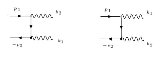
Figure 1: Lowest order Feynman diagrams describing two-photon annihilation of free electron and positron.

Note that

$$(\hat{p}_{1}+m)\hat{\epsilon}^{*}\,u(p_{1})=[2p_{1}\cdot\epsilon^{*}-\hat{\epsilon}^{*}(\hat{p}-m)]u(p_{1})=2p_{1}\cdot\epsilon^{*}u(p_{1}),$$

and (70) is equivalent to

$$M(e^{-}e^{+}\to 2\gamma)=e^{2}\bar{v}(p_{2})\left[\frac{2p_{1}\cdot\epsilon_{1}^{*}\,\hat{\epsilon}_{2}^{*}-\hat{\epsilon}^{*}_{2}\hat{k}_{1}\hat{\epsilon}^{*}_{1}}{2p_{1}\cdot k_{1}}+\frac{2p_{1}\cdot\epsilon_{2}^{*}\,\hat{\epsilon}_{1}^{*}-\hat{\epsilon}^{*}_{1}\hat{k}_{2}\hat{\epsilon}^{*}_{2}}{2p_{1}\cdot k_{2}}\right]u(p_{1}).$$ (71)

But $p_{1}\cdot k_{1}\approx m^{2}-\vec{p}\cdot\vec{k_{1}}$, $p_{1}\cdot k_{2}\approx m^{2}+\vec{p}\cdot\vec{k_{1}}$, and $p_{1}\cdot k_{1}\,p_{1}\cdot k_{2}\approx m^{4}$. This allows to rewrite (71) as follows

$$M(e^{-}e^{+}\to 2\gamma)=\frac{e^{2}}{2m^{4}}\bar{v}(p_{2})\left[(m^{2}+\vec{p}\cdot\vec{k}_{1})(2p_{1}\cdot\epsilon_{1}^{*}\,\hat{\epsilon}_{2}^{*}-\hat{\epsilon}^{*}_{2}\hat{k}_{1}\hat{\epsilon}^{*}_{1})+(m^{2}-\vec{p}\cdot\vec{k}_{1})(2p_{1}\cdot\epsilon_{2}^{*}\,\hat{\epsilon}_{1}^{*}-\hat{\epsilon}^{*}_{1}\hat{k}_{2}\hat{\epsilon}^{*}_{2})\right]u(p_{1})$$

$$\approx\frac{e^{2}}{2m^{4}}\bar{v}(p_{2})\left(\begin{array}[]{cc}0&2m^{2}a-m^{2}\bar{b}_{+}+\vec{p}\cdot\vec{k}_{1}\bar{b}_{-}\\ -2m^{2}a-m^{2}b_{+}+\vec{p}\cdot\vec{k}_{1}b_{-}&0\end{array}\right)u(p_{1}),$$ (74)

where

$$a=\vec{p}\cdot\vec{\epsilon}_{1}^{\,*}\,\vec{\sigma}\cdot\vec{\epsilon}_{2}^{\,*}+\vec{p}\cdot\vec{\epsilon}_{2}^{\,*}\,\vec{\sigma}\cdot\vec{\epsilon}_{1}^{\,*},\;\;b_{\pm}=\vec{\epsilon}_{1}^{\,*}\cdot\vec{\sigma}\,k_{2}\cdot\sigma\,\vec{\epsilon}_{2}^{\,*}\cdot\vec{\sigma}\pm\vec{\epsilon}_{2}^{\,*}\cdot\vec{\sigma}\,k_{1}\cdot\sigma\,\vec{\epsilon}_{1}^{\,*}\cdot\vec{\sigma},\;\;\bar{b}_{\pm}=\vec{\epsilon}_{1}^{\,*}\cdot\vec{\sigma}\,k_{2}\cdot\bar{\sigma}\,\vec{\epsilon}_{2}^{\,*}\cdot\vec{\sigma}\pm\vec{\epsilon}_{2}^{\,*}\cdot\vec{\sigma}\,k_{1}\cdot\bar{\sigma}\,\vec{\epsilon}_{1}^{\,*}\cdot\vec{\sigma},$$ (75)

and we have used the Coulomb gauge $\epsilon^{\mu}=(0,\vec{\epsilon})$ for photon polarization vectors, and the chiral representation for gamma matrices.

It is convenient, following Alekseev 2 , to express (74) in terms of two-component Pauli spinors. In the chiral representation, adopted in 3 ,

$$u(p_{1})=\left(\begin{array}[]{c}\sqrt{\sigma\cdot p_{1}}\,\xi\\ \sqrt{\bar{\sigma}\cdot p_{1}}\,\xi\end{array}\right)\approx\sqrt{m}\left(\begin{array}[]{c}\left(1-\frac{\vec{\sigma}\cdot\vec{p}}{2m}\right)\xi\\ \left(1+\frac{\vec{\sigma}\cdot\vec{p}}{2m}\right)\xi\end{array}\right),\;\;v(p_{2})=\left(\begin{array}[]{c}\hskip 8.53581pt\sqrt{\sigma\cdot p_{2}}\,\zeta\\ -\sqrt{\bar{\sigma}\cdot p_{2}}\,\zeta\end{array}\right)\approx\sqrt{m}\left(\begin{array}[]{c}\hskip 8.53581pt\left(1+\frac{\vec{\sigma}\cdot\vec{p}}{2m}\right)\zeta\\ -\left(1-\frac{\vec{\sigma}\cdot\vec{p}}{2m}\right)\zeta\end{array}\right),$$ (76)

where the approximate equalities, which are valid up to linear in $\vec{p}$ terms, follow from $\vec{p}_{1}=-\vec{p}_{2}=\vec{p}$ and

$$\sqrt{\sigma\cdot p}=\frac{\sigma\cdot p+m}{\sqrt{2(E+m)}}\approx\frac{1}{2\sqrt{m}}\left(2m-\vec{\sigma}\cdot\vec{p}\right),\;\;\;\sqrt{\bar{\sigma}\cdot p}=\frac{\bar{\sigma}\cdot p+m}{\sqrt{2(E+m)}}\approx\frac{1}{2\sqrt{m}}\left(2m+\vec{\sigma}\cdot\vec{p}\right).$$ (77)

Substituting (76) into (74) and discarding quadratic and higher in $\vec{p}$ terms, we get

$$M(e^{-}e^{+}\to 2\gamma)\approx\frac{e^{2}}{2m^{3}}\,\zeta^{+}\left(-4m^{2}a+m^{2}(\bar{b}_{+}-b_{+})+\vec{p}\cdot\vec{k}_{1}(b_{-}-\bar{b}_{-})+\frac{m}{2}\,[b_{+}+\bar{b}_{+},\,\vec{\sigma}\cdot\vec{p}\,]\right)\xi.$$ (78)

But, with required precision,

$$k_{1}\cdot(\sigma+\bar{\sigma})=k_{2}\cdot(\sigma+\bar{\sigma})=2m,\;\;k_{1}\cdot(\sigma-\bar{\sigma})=-2\vec{k}_{1}\cdot\vec{\sigma},\;\;k_{2}\cdot(\sigma-\bar{\sigma})=-2\vec{k}_{2}\cdot\vec{\sigma}=2\vec{k}_{1}\cdot\vec{\sigma},$$

and therefore

$$b_{\pm}-\bar{b}_{\pm}=2(\vec{\epsilon}^{\,*}_{1}\cdot\vec{\sigma}\,\vec{k}_{1}\cdot\vec{\sigma}\,\vec{\epsilon}^{\,*}_{2}\cdot\vec{\sigma}\mp\vec{\epsilon}^{\,*}_{2}\cdot\vec{\sigma}\,\vec{k}_{1}\cdot\vec{\sigma}\,\vec{\epsilon}^{\,*}_{1}\cdot\vec{\sigma}),\;\;b_{+}+\bar{b}_{+}=2m\left(\vec{\epsilon}^{\,*}_{1}\cdot\vec{\sigma}\,\vec{\epsilon}^{\,*}_{2}\cdot\vec{\sigma}+\vec{\epsilon}^{\,*}_{2}\cdot\vec{\sigma}\,\vec{\epsilon}^{\,*}_{1}\cdot\vec{\sigma}\right)=4m\,\vec{\epsilon}^{\,*}_{1}\cdot\vec{\epsilon}^{\,*}_{2}.$$ (79)

Hence $[b_{+}+\bar{b}_{+},\,\vec{\sigma}\cdot\vec{p}\,]=0$. To simplify further, we use the equality

$$\vec{\sigma}\cdot\vec{a}\,\vec{\sigma}\cdot\vec{b}=\vec{a}\cdot\vec{b}+i\vec{\sigma}\cdot(\vec{a}\times\vec{b}),$$ (80)

from which it follows that

$$\vec{\epsilon}^{\,*}_{1}\cdot\vec{\sigma}\,\vec{k}_{1}\cdot\vec{\sigma}\,\vec{\epsilon}^{\,*}_{2}\cdot\vec{\sigma}=i\left[\vec{\epsilon}^{\,*}_{2}\cdot(\vec{\epsilon}^{\,*}_{1}\times\vec{k}_{1})+i\vec{\sigma}\cdot[(\vec{\epsilon}^{\,*}_{1}\times\vec{k}_{1})\times\vec{\epsilon}^{\,*}_{2}]\right]=-i\vec{k}_{1}\cdot(\vec{\epsilon}^{\,*}_{1}\times\vec{\epsilon}^{\,*}_{2})-\vec{\sigma}\cdot\vec{k}_{1}\,\vec{\epsilon}^{\,*}_{1}\cdot\vec{\epsilon}^{\,*}_{2},$$ (81)

because $\vec{k}_{1}\cdot\vec{\epsilon}^{\,*}_{1}=0$ and $\vec{k}_{1}\cdot\vec{\epsilon}^{\,*}_{2}=-\vec{k}_{2}\cdot\vec{\epsilon}^{\,*}_{2}=0$. Using (81) in (79), we get

$$b_{+}-\bar{b}_{+}=-4i\,\vec{k}_{1}\cdot(\vec{\epsilon}^{\,*}_{1}\times\vec{\epsilon}^{\,*}_{2}),\;\;\;b_{-}-\bar{b}_{-}=-4\vec{\sigma}\cdot\vec{k}_{1}\,\vec{\epsilon}^{\,*}_{1}\cdot\vec{\epsilon}^{\,*}_{2},$$ (82)

and the final form of the two-photon annihilation amplitude, valid up to linear in $\vec{p}$ terms:

$$M(e^{-}e^{+}\to 2\gamma)\approx-\frac{2e^{2}}{m}\,\zeta^{+}\left[\vec{p}\cdot\vec{\epsilon}^{\,*}_{1}\,\vec{\sigma}\cdot\vec{\epsilon}^{\,*}_{2}+\vec{p}\cdot\vec{\epsilon}^{\,*}_{2}\,\vec{\sigma}\cdot\vec{\epsilon}^{\,*}_{1}-i\,\vec{k}_{1}\cdot(\vec{\epsilon}^{\,*}_{1}\times\vec{\epsilon}^{\,*}_{2})+\frac{1}{m^{2}}\,\vec{p}\cdot\vec{k}_{1}\,\vec{\sigma}\cdot\vec{k}_{1}\,\vec{\epsilon}^{\,*}_{1}\cdot\vec{\epsilon}^{\,*}_{2}\right]\xi.$$ (83)

This result is consistent with the ones given in 18 and 7 (after a typo is corrected in 7 which lead to mutual interchange of the photon polarization vectors).

IV Two-photon decays of $S$-wave positronium

To warm up, let’s calculate two-photon decay width of $S$-wave positronium. It is clear from (20) that the decay amplitude has the following form

$$M(^{2S+1}S_{J}\to 2\gamma)=\frac{1}{\sqrt{m}}\int\frac{d\vec{p}}{(2\pi)^{3}}\,\tilde{\psi}_{00}(\vec{p})\sum_{ss^{\prime}}[A^{(JM)}(-i\sigma_{2})]_{ss^{\prime}}M(e^{-}(s,\vec{p})\,e^{+}(s^{\prime},-\vec{p})\to 2\gamma).$$ (84)

In deriving prefactor in (84), we have taken into account the relativistic normalization of the one-particle states $|e^{-}(s,\vec{p})>=\sqrt{2E_{p}}\,a^{+}(s,\vec{p})|0>$ and that $E_{p}\approx m$ at desired accuracy.

It follows from (83) that

$$M(e^{-}(s,\vec{p})\,e^{+}(s,-\vec{p})\to 2\gamma)=\zeta^{s^{\prime}+}\Lambda\xi^{s},$$ (85)

where $\Lambda$ is some $2\times 2$ matrix acting on spinor indices. But

$$\sum_{ss^{\prime}}[A^{(JM)}(-i\sigma_{2})]_{ss^{\prime}}\zeta^{s^{\prime}+}\Lambda\xi^{s}=\mathrm{Tr}(\hat{\pi}_{A}^{(JM)}\Lambda),$$ (86)

with

$$\hat{\pi}_{A}^{(JM)}=\sum_{ss^{\prime}}[A^{(JM)}(-i\sigma_{2})]_{ss^{\prime}}\xi^{s}\zeta^{s^{\prime}+}$$ (87)

as a selector operator — a $2\times 2$ matrix in spinor space which discriminates between the singlet $J=0$ and triplet $J=1$ states.

To calculate $\hat{\pi}_{A}^{(JM)}$, let’s recall that the particle and antiparticle two-component spinors are (note the flipped nature of antiparticle spinors) 3

$$\xi^{\uparrow}=\left(\begin{array}[]{c}1\\ 0\end{array}\right),\;\;\xi^{\downarrow}=\left(\begin{array}[]{c}0\\ 1\end{array}\right),\;\;\zeta^{\uparrow}=\xi^{\downarrow}=\left(\begin{array}[]{c}0\\ 1\end{array}\right),\;\;\zeta^{\downarrow}=-\xi^{\uparrow}=\left(\begin{array}[]{c}-1\\ \hskip 5.69054pt0\end{array}\right).$$ (88)

Then, because the only non-zero components of $-i\sigma_{2}$ are $(-i\sigma_{2})_{\uparrow\downarrow}=-1$ and $(-i\sigma_{2})_{\downarrow\uparrow}=1$, we will have

$$\hat{\pi}_{A}^{(JM)}=\sum_{ss^{\prime}s^{\prime\prime}}A^{(JM)}_{ss^{\prime\prime}}(-i\sigma_{2})_{s^{\prime\prime}s^{\prime}}\xi^{s}\zeta^{s^{\prime}+}=\sum_{s}\left(-A^{(JM)}_{s\uparrow}\xi^{s}\zeta^{\downarrow+}+A^{(JM)}_{s\downarrow}\xi^{s}\zeta^{\uparrow+}\right),$$

and

$$\hat{\pi}_{A}^{(JM)}=A^{(JM)}_{\uparrow\uparrow}\left(\begin{array}[]{c}1\\ 0\end{array}\right)(1,0)+A^{(JM)}_{\downarrow\uparrow}\left(\begin{array}[]{c}0\\ 1\end{array}\right)(1,0)+A^{(JM)}_{\uparrow\downarrow}\left(\begin{array}[]{c}1\\ 0\end{array}\right)(0,1)+A^{(JM)}_{\downarrow\downarrow}\left(\begin{array}[]{c}0\\ 1\end{array}\right)(0,1)=\left(\begin{array}[]{cc}A^{(JM)}_{\uparrow\uparrow}&A^{(JM)}_{\uparrow\downarrow}\\ A^{(JM)}_{\downarrow\uparrow}&A^{(JM)}_{\downarrow\downarrow}\end{array}\right).$$ (89)

Note that $\hat{\pi}_{A}^{(JM)}$ and $A^{(JM)}$ act in different spaces — the first one acts on spinor indices and the second one acts on spin labels. However (89) indicates that in these spaces they act identically, that is

$$\hat{\pi}_{A}^{(00)}=\frac{1}{\sqrt{2}},\;\;\;\hat{\pi}_{A}^{(1M)}=\frac{1}{\sqrt{2}}\,\vec{n}_{M}\cdot\vec{\sigma}.$$ (90)

According to(83), at zeroth order

$$\Lambda^{(0)}=\frac{2ie^{2}}{m}\,\vec{k}_{1}\cdot(\vec{\epsilon}^{*}_{1}\times\vec{\epsilon}^{*}_{2})$$ (91)

doesn’t depend on $\vec{p}$. Then the remaining integral

$$\int\frac{d\vec{p}}{(2\pi)^{3}}\,\tilde{\psi}_{00}(\vec{p})=\psi(\vec{x}=0)$$

just gives the position space positronium wave function at the origin. Therefore

$$M(^{2S+1}S_{J}\to 2\gamma)=\frac{2ie^{2}}{m\sqrt{m}}\,\vec{k}_{1}\cdot(\vec{\epsilon}^{*}_{1}\times\vec{\epsilon}^{*}_{2})\,\psi(\vec{x}=0)\,\mathrm{T}r(\hat{\pi}^{(JM)}_{A}).$$ (92)

To calculate the decay rate, we should module square the amplitude (92), sum over the final state photon polarizations, average over the initial state positronium polarizations, and integrate over the Lorentz invariant final state phase space according to the general formula (overbar indicates the above mentioned summation and averaging over polarizations, $P=(M_{Ps},\vec{0})$ is the positronium 4-momentum)

$$d\Gamma(^{2S+1}L_{j}\to 2\gamma)=\frac{1}{2M_{Ps}}\,\overline{|M(^{2S+1}L_{j}\to 2\gamma)|^{2}}\,\frac{d\vec{k}_{1}}{(2\pi)^{3}2|\vec{k}_{1}|}\,\frac{d\vec{k}_{2}}{(2\pi)^{3}2|\vec{k}_{2}|}\,(2\pi)^{4}\delta^{(4)}(P-k_{1}-k_{2}).$$ (93)

In Coulomb gauge, the photon polarization sums can be performed by using

$$\sum_{\epsilon}\epsilon^{*i}(\vec{k})\epsilon^{j}(\vec{k})=\delta^{ij}-\frac{k^{i}\,k^{j}}{|\vec{k}|^{2}}.$$ (94)

Then (from here, it is assumed that repeated indices are implicitly summed over)

$$\sum_{\epsilon_{1}\,\epsilon_{2}}k_{1}^{i}k_{1}^{j}\epsilon^{imn}\epsilon^{im^{\prime}n^{\prime}}\epsilon_{1}^{*m}\epsilon_{2}^{*n}\epsilon_{1}^{m^{\prime}}\epsilon_{2}^{n^{\prime}}=\epsilon^{imn}\epsilon^{jmn}k_{1}^{i}k_{1}^{j}=2|\vec{k}_{1}|^{2},$$

and

$$\overline{|M(^{2S+1}S_{j}\to 2\gamma)|^{2}}=\frac{1}{2J+1}\sum_{\epsilon_{1}\,\epsilon_{2}}|M(^{2S+1}S_{j}\to 2\gamma)|^{2}=\frac{8e^{4}}{m^{3}}\,|\vec{k}_{1}|^{2}\,|\psi(\vec{x}=0)|^{2}\,|\mathrm{T}r(\hat{\pi}^{(JM)}_{A})|^{2}.$$ (95)

Since Pauli matrices are traceless and $\hat{\pi}^{(1M)}_{A}=\vec{n}_{M}\cdot\vec{\sigma}/\sqrt{2}$, we immediately get that the spin-triplet $S$-wave positronium (orthopositronium) doesn’t decay into two photons. Of course this is just what is expected from the $C$-parity conservation in electromagnetic decays: for the two-photon final state $C=(-1)^{2}=1$ while for the $L=0,S=1$ orthopositronium $C=(-1)^{L+S}=-1$.

For the spin-singlet $S$-wave positronium (parapositronium) $\hat{\pi}^{(00)}_{A}=1/\sqrt{2}$ and $\mathrm{Tr}(\hat{\pi}^{(00)}_{A})=\sqrt{2}$. Then from (93) and (95) we get (the first $1/2$ factor accounts for the identity of the final state photons)

$$\Gamma(^{1}S_{0}\to 2\gamma)=\frac{1}{2}\,\frac{e^{4}|\psi(\vec{x}=0)|^{2}}{\pi m^{4}}\int_{0}^{\infty}|\vec{k}_{1}|^{2}\delta(2m-2|\vec{k}_{1}|)\,d|\vec{k}_{1}|=\frac{e^{4}|\psi(\vec{x}=0)|^{2}}{4\pi m^{2}}=\frac{4\pi\alpha^{2}}{m^{2}}\,|\psi(\vec{x}=0)|^{2}.$$ (96)

What remains is to use

$$|\psi(\vec{x}=0)|^{2}=\frac{m^{3}\alpha^{3}}{8\pi},$$

valid for the positronium ground state (for radial excitations with the principal quantum number $n$ this quantity is $n^{3}$ times less), and obtain a well known result of Pirenne and Wheeler 19 ; 20

$$\Gamma(^{1}S_{0}\to 2\gamma)=\frac{m\alpha^{5}}{2}.$$ (97)

V Two-photon decays of $P$-wave positronium

Hydrogen-like wave function of positronium has the form 21

$$\psi_{nlm}(\vec{r})=\left[\frac{1}{2n}\left(\frac{2}{na_{0}}\right)^{3}\frac{(n-l-1)!}{(n+l)!}\right]^{1/2}\left(\frac{2r}{na_{0}}\right)^{l}e^{-r/na_{0}}\,\mathrm{L}_{n-l-1}^{2l+1}\left(\frac{2r}{na_{0}}\right)Y_{lm}(\theta,\phi),$$ (98)

where $a_{0}=2/(m\alpha)$ is the Bohr radius for positronium and

$$L_{n}^{m}(x)=(n+m)!\sum\limits_{k=0}^{n}\frac{(-1)^{k}}{k!(n-k)!(k+m)!}\,x^{k}$$ (99)

are associated Laguerre polynomials 22 .

Some words of caution is perhaps appropriate here. In the physical and mathematical literature one encounters two commonly used definitions of Laguerre and associated Laguerre polynomials. This constitutes a possible source of confusion to many students 21 ; 23 . In this paper we adopt the conventions of Arfken and Weber 22 , but one should bear in mind that conventions used can change from book to book. For example, Landau and Lifshits 24 use different conventions (namely, that of Spiegel 25 ) that changes the normalization coefficient, as well as the lower index from $n-l-1$ to $n+l$. Griffiths 26 follow Arfken and Weber when relating associated Laguerre polynomials to the ordinary Laguerre polynomials but uses different normalization in the definition of the latter, and this leads to different normalization coefficient than in (98).

It is clear from (98) that $\psi_{nlm}(\vec{0})=0$, if $l\neq 0$. Therefore the zeroth-order approximation of the previous section cannot be applied in the case of $P$-wave positronium decay and here our work in the pre-previous section pays off: as (83) shows

$$\Lambda=\Lambda^{(0)}+p^{j}\Lambda^{(1)j},$$ (100)

where $\Lambda^{(0)}$ is given by (91) and it doesn’t contribute to the $P$-wave positronium decay, while

$$\Lambda^{(1)j}=-\frac{2e^{2}}{m}\left[\vec{\sigma}\cdot\vec{\epsilon}_{2}^{\,*}\,\epsilon_{1}^{\,*j}+\vec{\sigma}\cdot\vec{\epsilon}_{1}^{\,*}\,\epsilon_{2}^{\,*j}+\frac{k_{1}^{j}}{m^{2}}\,\vec{\sigma}\cdot\vec{k_{1}}\,\vec{\epsilon}_{1}^{\,*}\cdot\vec{\epsilon}_{2}^{\,*}\right].$$ (101)

Positronium in the ${}^{1}P_{1}$ state with $S=0,L=1$ cannot decay into two photons due to $C$-parity conservation. It is reassuring that our formalism confirms this: $M(^{1}P_{1}\to 2\gamma)\sim p^{j}\tilde{\psi}^{i}(\vec{p})\,\mathrm{Tr}(\hat{\pi}_{C}^{(1M)i}\Lambda^{(1)j})=0$, because $\Lambda^{(1)j}$ is traceless and

$$\hat{\pi}_{C}^{(1M)i}=\sum_{ss^{\prime}}[C^{(1M)i}(-i\sigma_{2})]_{ss^{\prime}}\xi^{s}\zeta^{s^{\prime}+}=\frac{1}{\sqrt{2}}\,n_{M}^{i}$$

is proportional to the unit matrix.

As for the ${}^{3}P_{J}$ states, from (64) we have

$$M(^{3}P_{J}\to 2\gamma)=\frac{1}{\sqrt{m}}\,\mathrm{Tr}(\hat{\pi}_{B}^{(JM)i}\Lambda^{(1)j})\int\frac{d\vec{p}}{(2\pi)^{3}}\,p^{j}\tilde{\psi}^{i}(\vec{p}),$$ (102)

where

$$\hat{\pi}_{B}^{(JM)i}=\sum_{ss^{\prime}}[B^{(1M)i}(-i\sigma_{2})]_{ss^{\prime}}\xi^{s}\zeta^{s^{\prime}+}=\left\{\begin{array}[]{l}\frac{\sigma^{i}}{\sqrt{6}},\;\;\mathrm{if}\;\;(J,M)=(0,0),\\ \frac{1}{2}\epsilon^{ijk}n_{M}^{j}\sigma^{k},\;\;\mathrm{if}\;\;(J,M)=(1,M),\\ \frac{1}{\sqrt{2}}\,h_{M}^{ij}\sigma^{j},\;\;\mathrm{if}\;\;(J,M)=(2,M).\end{array}\right.$$ (103)

Let us first calculate the integral in (102). We have

$$\int\frac{d\vec{p}}{(2\pi)^{3}}\,p^{j}\tilde{\psi}^{i}(\vec{p})=\left.-i\nabla^{j}\psi^{i}(\vec{x})\right|_{\vec{x}=0}.$$ (104)

Since

$$\frac{1}{\sqrt{2}}\left(Y_{1,-1}(\theta,\phi)-Y_{1,1}(\theta,\phi)\right)=\sqrt{\frac{3}{4\pi}}\,\frac{x}{r},\;\;\frac{i}{\sqrt{2}}\left(Y_{1,-1}(\theta,\phi)+Y_{1,1}(\theta,\phi)\right)=\sqrt{\frac{3}{4\pi}}\,\frac{y}{r},\;\;Y_{1,0}(\theta,\phi)=\sqrt{\frac{3}{4\pi}}\,\frac{z}{r},$$

it follows from (23) and (98) that Cartesian wave function of the $P$-wave positronium is

$$\psi^{i}(\vec{x})=x^{i}\,\sqrt{\frac{3}{4\pi}\frac{1}{2n}\left(\frac{2}{na_{0}}\right)^{3}\frac{(n-2)!}{(n+1)!}}\,\frac{2}{na_{0}}\,e^{-r/na_{0}}\,\mathrm{L}_{n-2}^{3}\left(\frac{2r}{na_{0}}\right),$$ (105)

and therefore

$$\left.-i\nabla^{j}\psi^{i}(\vec{x})\right|_{\vec{x}=0}=-i\delta^{ij}\,\sqrt{\frac{3}{4\pi}\frac{1}{2n}\left(\frac{2}{na_{0}}\right)^{3}\frac{1}{(n-1)n(n+1)}}\,\frac{2}{na_{0}}\,\mathrm{L}_{n-2}^{3}(0).$$ (106)

But from (99)

$$\mathrm{L}_{n-2}^{3}(0)=\frac{(n+1)!}{(n-2)!\,3!}.$$ (107)

Combining (104), (106) and (107), we finally get

$$\int\frac{d\vec{p}}{(2\pi)^{3}}\,p^{j}\tilde{\psi}^{i}(\vec{p})=-i\delta^{ij}\,\sqrt{\frac{n^{2}-1}{96\pi n^{5}}(m\alpha)^{5}},$$ (108)

and

$$M(^{3}P_{J}\to 2\gamma)=-im^{2}\sqrt{\frac{(n^{2}-1)\alpha^{5}}{96\pi n^{5}}}\,\mathrm{Tr}(\hat{\pi}_{B}^{(JM)i}\Lambda^{(1)i}).$$ (109)

Now it’s time to calculate traces in (109) and this can be easily done by using (80). The results are

$$\mathrm{Tr}(\hat{\pi}_{B}^{(00)i}\Lambda^{(1)i})=-2\sqrt{6}\,\frac{e^{2}}{m}\,\vec{\epsilon}^{\,*}_{1}\cdot\vec{\epsilon}^{\,*}_{2},\;\;\mathrm{Tr}(\hat{\pi}_{B}^{(2M)i}\Lambda^{(1)i})=-2\sqrt{2}\,\frac{e^{2}}{m}\left(2h_{M}^{ij}\epsilon^{\,*i}_{1}\epsilon^{\,*j}_{2}+\frac{\vec{\epsilon}^{\,*}_{1}\cdot\vec{\epsilon}^{\,*}_{2}}{m^{2}}\,h_{M}^{ij}k_{1}^{i}k_{1}^{j}\right),$$ (110)

and

$$\mathrm{Tr}(\hat{\pi}_{B}^{(1M)i}\Lambda^{(1)i})=-\frac{2e^{2}}{m}\left[\vec{\epsilon}^{\,*}_{2}\cdot(\vec{\epsilon}^{\,*}_{1}\times\vec{n}_{M})+\vec{\epsilon}^{\,*}_{1}\cdot(\vec{\epsilon}^{\,*}_{2}\times\vec{n}_{M})+\frac{\vec{\epsilon}^{\,*}_{1}\cdot\vec{\epsilon}^{\,*}_{2}}{m^{2}}\,\vec{k}_{1}\cdot(\vec{k}_{1}\times\vec{n}_{M})\right]=0.$$ (111)

The last result implies that ${}^{3}P_{1}$ state doesn’t decay into two-photons although it has positive $C$-parity. This time the decay is forbidden by the Landau-Yang theorem 27 ; 28 which states that two real photons, when referred to their center of mass frame, cannot be in a state of total angular momentum one. The proof of the theorem is simple and only makes use of such basic concepts as the superposition principle, Bose statistics and transversality of real photons, and rotational invariance 29 . As we see, our formalism correctly reproduces this selection rule too.

In the case of ${}^{3}P_{0}$ state, the decay amplitude equals to

$$M(^{3}P_{0}\to 2\gamma)=i\frac{me^{2}}{2}\sqrt{\frac{(n^{2}-1)\alpha^{5}}{\pi n^{5}}}\,\vec{\epsilon}^{\,*}_{1}\cdot\vec{\epsilon}^{\,*}_{2}.$$ (112)

To calculate the decay rate, we should module square this amplitude and sum over the photon polarizations using (94). In this way we get

$$\sum_{\epsilon_{1},\epsilon_{2}}|\vec{\epsilon}^{\,*}_{1}\cdot\vec{\epsilon}^{\,*}_{2}|^{2}=\sum_{\epsilon_{1},\epsilon_{2}}\epsilon_{1}^{\,*i}\epsilon_{1}^{j}\,\epsilon_{2}^{\,*i}\epsilon_{2}^{j}=2,$$ (113)

and

$$\overline{|M(^{3}P_{0}\to 2\gamma)|^{2}}=\sum_{\epsilon_{1},\epsilon_{2}}|M(^{3}P_{0}\to 2\gamma)|^{2}=8\pi m^{2}\,\frac{n^{2}-1}{n^{5}}\,\alpha^{7}.$$ (114)

Eq.(93) indicates that the decay rate and the corresponding squared amplitude are related by

$$\frac{d\Gamma}{d\Omega}=\frac{1}{64\pi^{2}M_{Ps}}\,\overline{|M|^{2}}.$$ (115)

In our case the squared amplitude (114) is just a constant, the integration of (115) is trivial and we finally get (the factor $1/2$ accounts for the identical final state photons)

$$\Gamma(^{3}P_{0}\to 2\gamma)=\frac{1}{2}\int\frac{d\Gamma(^{3}P_{0}\to 2\gamma)}{d\Omega}\,d\Omega=\frac{n^{2}-1}{8n^{5}}\,m\alpha^{7}.$$ (116)

The amplitude for the ${}^{3}P_{2}\to 2\gamma$ decay is more complicated: from (109) and (110) we get

$$M(^{3}P_{2}\to 2\gamma)=ie^{2}m\sqrt{\frac{(n^{2}-1)\alpha^{5}}{12\pi n^{5}}}\left(2h_{M}^{ij}\epsilon^{\,*i}_{1}\epsilon^{\,*j}_{2}+\frac{\vec{\epsilon}^{\,*}_{1}\cdot\vec{\epsilon}^{\,*}_{2}}{m^{2}}\,h_{M}^{ij}k_{1}^{i}k_{1}^{j}\right).$$ (117)

The next step is to module square this amplitude, perform the photon polarization sums, and average over the initial state positronium polarization (that is sum over $M$ and divide by $2J+1=5$). This requires some algebra, somewhat simplified by the fact that $h_{M}^{ij}$ polarization tensors are traceless, symmetric and normalized to one. Besides, $\vec{k}_{1}^{\,2}\approx m^{2}$. After the dust settles we find

$$\overline{|M(^{3}P_{2}\to 2\gamma)|^{2}}=\frac{8\pi(n^{2}-1)m^{2}\alpha^{7}}{15n^{5}}\sum_{M}\left(2-4h_{M}^{ij}h_{M}^{\,*im}\,\frac{k_{1}^{j}k_{1}^{m}}{m^{2}}+h_{M}^{ij}h_{M}^{\,*mn}\,\frac{k_{1}^{i}k_{1}^{j}k_{1}^{m}k_{1}^{n}}{m^{4}}\right).$$ (118)

Then from (115) we get

$$\Gamma(^{3}P_{2}\to 2\gamma)=\frac{m\alpha^{7}}{32\pi}\,\frac{n^{2}-1}{15n^{5}}\sum_{M}\left(8\pi-4h_{M}^{ij}h_{M}^{\,*im}\int\frac{k_{1}^{j}k_{1}^{m}}{m^{2}}\,d\Omega+h_{M}^{ij}h_{M}^{\,*mn}\int\frac{k_{1}^{i}k_{1}^{j}k_{1}^{m}k_{1}^{n}}{m^{4}}\,d\Omega\right).$$ (119)

The integrals involved give the completely symmetric second and forth rank tensors respectively. As the integrands don’t contain any external vector or tensor, these tensors should be expressible in terms of $\delta^{ij}$ tensors only. Thus (the last expression is obtained by symmetrization of $\delta^{ij}\delta^{mn}$)

$$\int\frac{k_{1}^{j}k_{1}^{m}}{m^{2}}\,d\Omega=A\delta^{jm},\;\;\;\int\frac{k_{1}^{i}k_{1}^{j}k_{1}^{m}k_{1}^{n}}{m^{4}}\,d\Omega=B(\delta^{ij}\delta^{mn}+\delta^{im}\delta^{jn}+\delta^{in}\delta^{jm}).$$

To find the unknown coefficients $A$ and $B$, we simply contract these tensors:

$$4\pi=\int\frac{k_{1}^{j}k_{1}^{j}}{m^{2}}\,d\Omega=A\delta^{jj}=3A,\;\;\;4\pi=\int\frac{k_{1}^{i}k_{1}^{i}k_{1}^{m}k_{1}^{m}}{m^{4}}\,d\Omega=B(\delta^{ii}\delta^{mm}+\delta^{im}\delta^{im}+\delta^{im}\delta^{im})=15B.$$

Therefore $A=4\pi/3$, $B=4\pi/15$ and

$$\int\frac{k_{1}^{j}k_{1}^{m}}{m^{2}}\,d\Omega=\frac{4\pi}{3}\,\delta^{jm},\;\;\;\int\frac{k_{1}^{i}k_{1}^{j}k_{1}^{m}k_{1}^{n}}{m^{4}}\,d\Omega=\frac{4\pi}{15}\,(\delta^{ij}\delta^{mn}+\delta^{im}\delta^{jn}+\delta^{in}\delta^{jm}).$$ (120)

It remains to substitute (120) integrals into (119) and remember that $h_{M}^{ij}$ tensors are traceless and normalized to one. As a result, we get

$$\Gamma(^{3}P_{2}\to 2\gamma)=\frac{m\alpha^{7}}{32\pi}\,\frac{n^{2}-1}{15n^{5}}\sum_{M}\left(8\pi-\frac{16\pi}{3}+\frac{8\pi}{15}\right)=\frac{n^{2}-1}{30n^{5}}\,m\alpha^{7}.$$ (121)

Our final results (116) and (121) are precisely the ones obtained by Tumanov 1 and Alekseev 2 . In particular, for the $n=2$ states the decay widths are

$$\Gamma(2\,^{3}P_{0}\to 2\gamma)=\frac{3}{256}\,m\alpha^{7},\;\;\;\Gamma(2\,^{3}P_{2}\to 2\gamma)=\frac{1}{320}\,m\alpha^{7}.$$ (122)

VI Concluding remarks

We hope that this rather detailed presentation of two-photon decays of $P$-wave positronium will be helpful for quantum field theory students. The standard approach used in this note is lucid enough and well motivated. However thoughtful students can feel a necessity in a more powerful and complete framework.

Our main assumption was a factorization of the bound state dynamics from the annihilation process. However such an approach violates energy conservation: electron and positron that annihilate are on-shell and thus their total energy is greater than $M_{Ps}$. Of course for non-relativistic systems, like positronium, the difference is of the order of $\alpha^{2}$ and can be neglected at lowest order. However thoughtful students can wonder how the off-shellness of constituents can be reintroduced perturbatively at higher order calculations (an example can be found in 29A ).

The ratio $\Gamma(2\,^{3}P_{0}\to 2\gamma)/\Gamma(2\,^{3}P_{2}\to 2\gamma)=15/4$, which follows from the previous section, is often quoted in the context of quarkonium decays. However it should be beared in mind that for quarkonia relativistic corrections are important and can lead to significant modification of this ratio 18 .

Another potential source of concern is subtle consequences of gauge invariance. As was shown by Low 30 , gauge invariance and analyticity implies that the decay amplitude of neutral bosons vanishes in the soft photon limit. Since the standard factorization treats intermediate charged states as on-shell, emission of soft photons by this particles is accompanied by well known infrared singularities. Although the standard treatment ensures the cancellation of these infrared singularities, the amplitude, for example, for the $Ps\to 3\gamma$ decay, being finite, doesn’t vanish in the soft photon limit, in contradiction to the Low’s theorem 31 . Special efforts to correctly account for binding energy corrections are needed to reinforce the theorem 31 .

We hope that the two-photon decays of $P$-wave positronium can serve for attentive students as a vista to a vast new land called a bound state problem in relativistic quantum field theory. As an initial guidebook into this interesting land, we recommend relatively recent PhD thesis 32 .

References

• (1) K. A. Tumanov, Quantum electrodynamics in configuration representation. \Romannum5: two-photon annihilation of positronium. Zh. Eksp. Teor. Fiz.  25, 385-392 (1953).
• (2) A. I. Alekseev, Two-photon annihilation of positronium in the P-state. Sov. Phys. JETP 34, 826-830 (1958).
• (3) M. E. Peskin and D. V. Schroeder, An introduction to quantum field theory (Perseus Books, Reading, Massachusetts, 1995).
• (4) V. A. Novikov, L. B. Okun, M. A. Shifman, A. I. Vainshtein, M. B. Voloshin and V. I. Zakharov, Charmonium and Gluons: Basic Experimental Facts and Theoretical Introduction, Phys. Rept.  41, 1-133 (1978).
• (5) R. Barbieri, R. Gatto and R. Kögerler, Calculation of the Annihilation Rate of P-Wave Quark - anti-Quark Bound States, Phys. Lett.  60B, 183-188 (1976).
• (6) Zhong-Zhi Xianyu, A Complete Solution to Problems in “An Introduction to Quantum Field Theory”by Peskin and Schroeder. https://zzxianyu.files.wordpress.com/2017/01/peskin_problems.pdf (accessed july 6, 2018).
• (7) S. U. Chung, Two-Photon Amplitudes of Quarkonia in Helicity Formalism. BNL preprint BNL-QGS-02-011, 2002.
• (8) M. Jacob and G. C. Wick, On the general theory of collisions for particles with spin, Annals Phys.  7, 404-428 (1959) [Annals Phys.  281, 774-799 (2000)].
• (9) C. Itzykson and J.-B. Zuber, Quantum Field Theory (McGraw-Hill, New York, 1980).
• (10) J. M. Jauch and F. Rohrlich, The theory of photons and electrons. The relativistic quantum field theory of charged particles with spin one-half (Springer-Verlag, Berlin, 1980).
• (11) C. Smith, Bound State Description in Quantum Electrodynamics and Chromodynamics, PhD dissertation, Louvain-la-Neuve, 2002. https://cp3.irmp.ucl.ac.be/upload/theses/phd/smith.pdf (accessed july 6, 2018).
• (12) C. R. Munz, Two photon decays of mesons in a relativistic quark model, Nucl. Phys. A 609, 364-376 (1996).
• (13) G. L. Wang, Annihilation rate of heavy 0++ P-wave quarkonium in relativistic Salpeter method, Phys. Lett. B 653, 206-209 (2007).
• (14) H. W. Crater, C. Y. Wong and P. Van Alstine, Tests of two-body Dirac equation wave functions in the decays of quarkonium and positronium into two photons, Phys. Rev. D 74, 054028 (2006).
• (15) C. W. Hwang and R. S. Guo, Two-photon and two-gluon decays of p-wave heavy quarkonium using a covariant light-front approach, Phys. Rev. D 82, 034021 (2010).
• (16) S. N. Gupta, J. M. Johnson and W. W. Repko, Relativistic two photon and two gluon decay rates of heavy quarkonia, Phys. Rev. D 54, 2075-2080 (1996).
• (17) J. P. Lansberg and T. N. Pham, Effective Lagrangian for Two-photon and Two-gluon Decays of P-wave Heavy Quarkonium chi(c0,2) and chi(b0,2) states, Phys. Rev. D 79, 094016 (2009).
• (18) G. T. Bodwin, NRQCD: Fundamentals and applications to quarkonium decay and production, Int. J. Mod. Phys. A 21, 785-792 (2006).
• (19) J. P. Ma and Q. Wang, Corrections for two photon decays of chi(c0) and chi(c2) and color octet contributions, Phys. Lett. B 537, 233-240 (2002).
• (20) M. Ambrogiani et al., Study of the gamma gamma decays of the $\chi_{c2}\,(1\,^{3}P_{2})$ and $\chi_{c0}\,(1\,^{3}P_{0})$ charmonium resonances, Phys. Rev. D 62, 052002 (2000).
• (21) K. M. Ecklund et al. [CLEO Collaboration], Two-Photon Widths of the chi(cJ) States of Charmonium, Phys. Rev. D 78, 091501 (2008).
• (22) E. E. Salpeter and H. A. Bethe, A Relativistic equation for bound state problems, Phys. Rev.  84, 1232-1242 (1951).
• (23) N. Nakanishi, A General survey of the theory of the Bethe-Salpeter equation, Prog. Theor. Phys. Suppl.  43, 1-81 (1969).
• (24) Z. K. Silagadze, Wick-Cutkosky model: An Introduction, hep-ph/9803307.
• (25) R. Barbieri and E. Remiddi, Solving the Bethe-Salpeter Equation for Positronium, Nucl. Phys. B 141, 413-422 (1978).
• (26) W. E. Caswell and G. P. Lepage, Reduction of the Bethe-Salpeter Equation to an Equivalent Schrödinger Equation, With Applications, Phys. Rev. A 18, 810-819 (1978).
• (27) V. Devanathan, Angular Momentum Techniques in Quantum Mechanics (Kluwer Academic Publishers, New York, 2002).
• (28) T. Kinoshita and G. P. Lepage, Quantum electrodynamics for nonrelativistic systems and high precision determinations of alpha, Adv. Ser. Direct. High Energy Phys.  7, 81-91 (1990).
• (29) C. Patrignani et al. [Particle Data Group], Review of Particle Physics, Chin. Phys. C 40, 100001 (2016), p. 557.
• (30) T. Han, J. D. Lykken and R. J. Zhang, On Kaluza-Klein states from large extra dimensions, Phys. Rev. D 59, 105006 (1999).
• (31) Z. P. Li, F. E. Close and T. Barnes, Relativistic effects in gamma gamma decays of P wave positronium and q anti-q systems, Phys. Rev. D 43, 2161-2170 (1991).
• (32) S. Berko and H. N. Pendleton, Positronium, Ann. Rev. Nucl. Part. Sci.  30, 543-581 (1980).
• (33) D. B. Cassidy, Experimental progress in positronium laser physics, Eur. Phys. J. D 72, 53 (2018).
• (34) C. E. Burkhardt and J. J. Leventhal, Foundations of Quantum Physics (Springer, New York, 2008).
• (35) G. B. Arfken and H. J. Weber, Mathematical Methods for Physicists (Harcourt, New York, 2001).
• (36) C. E. Burkhardt and J. J. Leventhal, Topics in Atomic Physics (Springer, New York, 2006)
• (37) L. D. Landau and E. M. Lifshits, Quantum Mechanics: Non-Relativistic Theory (Butterworth-Heinemann, Oxford, 1992).
• (38) M. R. Spiegel, Mathematical Handbook of Formulas and Tables (McGraw-Hill, New York, 1998).
• (39) D. J. Griffiths, Introduction to Quantum Mechanics (Prentice Hall, New York, 1995).
• (40) L. D. Landau, On the angular momentum of a system of two photons, Dokl. Akad. Nauk Ser. Fiz.  60, 207-209 (1948).
• (41) C. N. Yang, Selection Rules for the Dematerialization of a Particle Into Two Photons, Phys. Rev.  77, 242-245 (1950).
• (42) O. Nachtmann, Elementary Particle Physics: Concepts and Phenomena (Springer-Verlag, Berlin, 1990).
• (43) J. Pestieau, C. Smith and S. Trine, Positronium decay: Gauge invariance and analyticity, Int. J. Mod. Phys. A 17, 1355-1398 (2002).
• (44) F. E. Low, Bremsstrahlung of very low-energy quanta in elementary particle collisions, Phys. Rev.  110, 974-977 (1958).
• (45) J. Pestieau and C. Smith, Soft photon spectrum in orthopositronium and vector quarkonium decays, Phys. Lett. B 524, 395-399 (2002).