Operator Splitting Performance Estimation: Tight contraction factors and optimal parameter selection

Abstract

We propose a methodology for studying the performance of common splitting methods through semidefinite programming. We prove tightness of the methodology and demonstrate its value by presenting two applications of it. First, we use the methodology as a tool for computer-assisted proofs to prove tight analytic contraction factors for Douglas–Rachford splitting that are likely too complicated for a human to find bare-handed. Second, we use the methodology as an algorithmic tool to computationally select the optimal splitting method parameters by solving a series of semidefinite programs.

1 Introduction

Consider the fixed-point iteration in a real Hilbert space $\mathcal{H}$

$$z^{k+1}=Tz^{k},$$

where $T\colon\mathcal{H}\rightarrow\mathcal{H}$. We say $\rho<1$ is a contraction factor of $T$ if

$$\|Tx-Ty\|\leq\rho\|x-y\|$$

for all $x,y\in\mathcal{H}$. We ask the question: given a set of assumptions, what is the best (tight) contraction factor one can prove? In this work, we present the operator splitting performance estimation problem (OSPEP), a methodology for studying contraction factors of forward-backward splitting (FBS), Douglas–Rachford splitting (DRS), and Davis–Yin splitting (DYS).

First, we present the OSPEP problem, the infinite-dimensional non-convex optimization problem of finding the best (smallest) contraction factor given a set of assumptions on the operators. Following the technique of Drori and Teboulle [20], we reformulate the problem into a finite-dimensional convex semidefinite program (SDP). We then establish tightness (exactness) of this reformulation with interpolation conditions.

Next, we demonstrate the value of OSPEP through two uses. First, we use OSPEP as a tool for computer-assisted proofs to prove tight analytic contraction factors for DRS. The results are tight in that they have exact matching lower bounds. The proofs are computer-assisted in that their discoveries were assisted by a computer, but their verifications do not require a computer. Second, we use OSPEP as an algorithmic tool to automatically select the optimal splitting method parameters.

The tightness guarantee and flexibility make OSPEP a powerful tool. Due to tightness, OSPEP can provide both positive and negative results. The flexibility allows users to pick and choose assumptions from a set of standard assumptions.

1.1 Organization and contribution

Section 2 presents operator interpolation, later used in Section 3 to establish tightness. Section 3 presents the OSPEP methodology, an exact transformation of the problem of finding the best contraction factor into a convex SDP, and provides tightness guarantees. Section 4 presents tight analytic contraction factors for DRS under assumptions considered in [25, 53] using OSPEP as a tool for computer-assisted proofs. Section 5 presents an automatic parameter selection method using OSPEP as an algorithmic tool. Section 6 concludes the paper.

The main contribution of this work is twofold. The first is analyzing the performance of monotone splitting methods using SDPs with tightness guarantees. The overall formulation generally follows from the technique of Drori and Teboulle [20] and the prior work discussed in Section 1.2. The tightness, established with the operator interpolation results of Sections 2, is a novel theoretical contribution. The second contribution is the techniques of Sections 4 and 5, an illustration of how to use the proposed methodology. Although we do consider the results of Sections 4 and 5 to be interesting and valuable, we view the technique, rather than the result, to be the second major contribution.

The major and minor contributions of this work are, to the best of our knowledge, novel in the following sense. The tightness of Section 3 is new. The technique of Section 4 is the first use of computer-assisted proofs to obtain provably tight rates for monotone operator splitting methods. The tight results of Section 4 improve upon the prior results of [25, 53]. The technique of Section 5 is the first use of automatic parameter selection that is optimal with respect to the algorithm and assumptions.

1.2 Prior work

FBS was first stated in the operator theoretic language in [7, 55]. The projected gradient method presented in [28, 44] served as a precursor to FBS. Peaceman-Rachford spitting (PRS) was first presented in [56, 34, 47], and DRS was first presented in [18, 47]. DYS was first presented in [16]. Forward-Douglas–Rachford splitting of Raguet, Fadili, Peyré, and Brineño-Arias [61, 5, 60] served as a precursor to DYS.

What we call interpolation in this work is also called extension. The maximal monotone extension theorem, which we later state as Fact 1, is well known, and it follows from a standard application of Zorn’s lemma. Reich [62], Bauschke [1], Reich and Simons [63], Bauschke, Wang, and Yao [3, 4, 83], and Crouzeix and Anaya [13, 12, 11] have studied more concrete and constructive extension theorems for maximal monotone, nonexpansive, and firmly-nonexpansive operators using tools from monotone operator theory.

Contraction factors and linear convergence for first-order methods have been a subject of intense study. Surprisingly, many of the published contraction factors are not tight. For FBS, Mercier, [51, p. 25], Tseng [77], Chen and Rockafellar [8], and Bauschke and Combettes [2, Section 26.5] proved linear rates of convergence, but did not provide exact matching lower bounds. Taylor, Hendrickx, and Glineur showed tight contraction factors and provided exact matching lower bounds [74]. For DRS, Lions and Mercier [47] and Davis and Yin [15] proved linear rates of convergence, but did not provide exact matching lower bounds. Giselsson and Boyd [26, 27], Giselsson [24, 25], and Moursi and Vandenberghe [53] proved linear rates of convergence and provided exact matching lower bounds for certain cases. ADMM is a splitting method closely related to DRS. Deng and Yin [17], Giselsson and Boyd [26, 27], Nishihara et al. [54], França and Bento [21], Hong and Luo [33], Han, Sun, and Zhang [32], and Chen et al. [9] proved linear rates of convergence for ADMM. Matching lower bounds are provided only in [27]. Further, [24] provides matching lower bounds to the rates in [26]. Ghadimi et al. [22, 23] and Teixeira et al. [75, 76] proved linear rates of convergence and provided matching lower bounds for ADMM applied to quadratic problems. For DYS, Davis and Yin [16], Yan [84], Pedregosa and Gidel [59], and Pedregosa, Fatras, and Casotto [58] proved linear rates of convergence, but did not provide exact matching lower bounds. Pedegrosa [57] analyzed sublinear convergence, but not contraction factors.

Analyzing convex optimization algorithms by formulating the analysis as an SDP has been a rapidly growing area of research in the past 5 years. Past work analyzed convex optimization algorithms, and, to the best of our knowledge, analyzing the performance of monotone operator splitting methods with SDPs or any form of computer-assisted proof is new. (After the initial version of this paper was made public on arXiv, several papers citing our work followed up on our results and used SDPs to analyze other monotone operator splitting methods [29, 30, 31, 69, 82, 68].) Drori and Teboulle [20] and Taylor, Hendrickx, and Glineur [71, 73] presented the performance estimation problem (PEP) methodology. Our work generally follows the techniques presented by Drori and Teboulle [20] while contributing by establishing tightness. Lieder [45] applied the PEP approach to analyze the Halpern iteration without an a priori guarantee of tightness. Lessard, Recht, and Packard [43] leveraged techniques from control theory and used integral quadratic constraints (IQC) for finding Lyapunov functions for analyzing convex optimization algorithms. The IQC and PEP approaches were recently linked by Taylor, Van Scoy, and Lessard [70]. Finally, Nishihara et al. [54] and França and Bento [21] used IQC to the analyze ADMM.

Finally, both IQC and PEP approaches allowed designing new methods for particular problem settings. For example, the optimized gradient method by Kim and Fessler [35, 36, 37, 38, 39, 40] (first numerical version by Drori and Teboulle [20]) was developed using PEPs and enjoys the best possible worst-case guarantee on the final objective function accuracy after a fixed number of iteration, as showed by Drori [19]. On the other hand, the IQC framework was used by Van Scoy et al. [81] for developing the triple momentum method, the first-order method with the fastest known convergence rate for minimizing a smooth strongly convex function.

1.3 Preliminaries

We now quickly review standard results and set up the notation. We follow standard notation [66, 2]. Write $\mathcal{H}$ for a real Hilbert space equipped with a (symmetric) inner product $\langle\cdot,\cdot\rangle$. Write $\mathbb{S}_{+}^{n}$ for the set of $n\times n$ symmetric positive semidefinite matrices. Write $M\succeq 0$ if and only if $M\in\mathbb{S}_{+}^{n}$.

We say $A$ is an operator on $\mathcal{H}$ and write $A\colon\mathcal{H}\rightrightarrows\mathcal{H}$ if $A$ maps a point in $\mathcal{H}$ to a subset of $\mathcal{H}$. So $A(x)\subset\mathcal{H}$ for all $x\in\mathcal{H}$. For simplicity, we also write $Ax=A(x)$. Write $I\colon\mathcal{H}\rightarrow\mathcal{H}$ for the identity operator. We say $A\colon\mathcal{H}\rightrightarrows\mathcal{H}$ is monotone if

$$\langle Ax-Ay,x-y\rangle\geq 0$$

for all $x,y\in\mathcal{H}$. To clarify, the inequality means $\langle u-v,x-y\rangle\geq 0$ for all $u\in Ax$ and $v\in Ay$. We say $A\colon\mathcal{H}\rightrightarrows\mathcal{H}$ is $\mu$-strongly monotone if

$$\langle Ax-Ay,x-y\rangle\geq\mu\|x-y\|^{2},$$

where $\mu\in(0,\infty)$. We say a single-valued operator $A\colon\mathcal{H}\to\mathcal{H}$ is $\beta$-cocoercive if

$$\langle Ax-Ay,x-y\rangle\geq\beta\|Ax-Ay\|^{2},$$

where $\beta\in(0,\infty)$. We say a single-valued operator $A\colon\mathcal{H}\to\mathcal{H}$ is $L$-Lipschitz if

$$\|Ax-Ay\|\leq L\|x-y\|$$

where $L\in(0,\infty)$. A monotone operator is maximal if it cannot be properly extended to another monotone operator. The resolvent of an operator $A$ is $J_{\alpha A}=(I+\alpha A)^{-1}$, where $\alpha>0$. We say a single-valued operator $T\colon\mathcal{H}\rightarrow\mathcal{H}$ is contractive if it is $\rho$-Lipschitz with $\rho<1$. We say $x^{\star}$ is a fixed point of $T$ if $x^{\star}=Tx^{\star}$.

Davis–Yin splitting (DYS) encodes solutions to

$$\begin{array}[]{ll}\underset{x\in\mathcal{H}}{\mbox{find}}&0\in(A+B+C)x\end{array}$$

where $A$, $B$, and $C$ are maximal monotone and $C$ is single-valued, as fixed points of

(1) $$T(z;A,B,C,\alpha,\theta)=z-\theta J_{\alpha B}z+\theta J_{\alpha A}(2J_{\alpha B}-I-\alpha CJ_{\alpha B})z$$

where $\alpha>0$ and $\theta\neq 0$. FBS and DRS are special cases of DYS; when $C=0$ DYS reduces to DRS, and when $B=0$ DYS reduces to FBS. Therefore, our analysis on DYS directly applies to FBS and DRS.

2 Operator interpolation

Let $\mathcal{Q}$ be a class of operators, and let $\mathcal{I}$ be an arbitrary index set. We say a set of duplets $\{(x_{i},q_{i})\}_{i\in\mathcal{I}}$, where $x_{i},q_{i}\in\mathcal{H}$ for all $i\in\mathcal{I}$, is $\mathcal{Q}$-interpolable if there is an operator $Q\in\mathcal{Q}$ such that $q_{i}\in Qx_{i}$ for all $i\in\mathcal{I}$. In this case, we call $Q$ an interpolation of $\{(x_{i},q_{i})\}_{i\in\mathcal{I}}$. In this section, we present conditions that characterize when a set of duplets is interpolable with respect to the class of operators listed in Table 1 and their intersections.

Class	Description
$\mathcal{M}$	maximal monotone operators
$\mathcal{M}_{\mu}$	$\mu$-strongly monotone maximal monotone operators
$\mathcal{L}_{L}$	$L$-Lipschitz operators
$\mathcal{C}_{\beta}$	$\beta$-cocoercive operators

Table 1: Operator classes for which we analyze interpolation. The parameters $\mu$, $L$, and $\beta$ are in $(0,\infty)$. Note that $\mathcal{M}_{\mu}\subset\mathcal{M}$ for any $\mu>0$, $\mathcal{C}_{\beta}\subset\mathcal{M}$ for any $\beta>0$, but $\mathcal{L}_{L}\not\subset\mathcal{M}$ for any $L>0$.

2.1 Interpolation with one class

We now present interpolation results for the classes $\mathcal{M}$, $\mathcal{M}_{\mu}$, $\mathcal{L}_{L}$, and $C_{\beta}$.

Fact 1 (Maximal monotone extension theorem [2, Theorem 20.21]).

$\{(x_{i},q_{i})\}_{i\in\mathcal{I}}$ is $\mathcal{M}$-interpolable if and only if

$$\langle q_{i}-q_{j},x_{i}-x_{j}\rangle\geq 0\qquad\forall i,j\in\mathcal{I}.$$

Proposition 1.

Let $\mu\in(0,\infty)$. Then $\{(x_{i},q_{i})\}_{i\in\mathcal{I}}$ is $M_{\mu}$-interpolable if and only if

$$\langle q_{i}-q_{j},x_{i}-x_{j}\rangle\geq\mu\|x_{i}-x_{j}\|^{2}\qquad\forall i,j\in\mathcal{I}.$$

Proof.

With Fact 1, the proof follows from a sequence of equivalences:

$$\forall i,j\in\mathcal{I},\,\langle q_{i}-q_{j},x_{i}-x_{j}\rangle \geq\mu\|x_{i}-x_{j}\|^{2}$$

$$\quad\Leftrightarrow\quad\forall i,j\in\mathcal{I},\langle(q_{i}-\mu x_{i})-(q_{j}-\mu x_{j}),x_{i}-x_{j}\rangle\geq 0$$

$$\quad\Leftrightarrow\quad\exists R\in\mathcal{M},\forall i\in\mathcal{I},(q_{i}-\mu x_{i})\in Rx_{i}$$

$$\quad\Leftrightarrow\quad\exists Q\in\mathcal{M}_{\mu},Q=R+\mu I,\,\forall i\in\mathcal{I},\,q_{i}\in Qx_{i}.$$

Proposition 2.

Let $\beta\in(0,\infty)$. Then $\{(x_{i},q_{i})\}_{i\in\mathcal{I}}$ is $\mathcal{C}_{\beta}$-interpolable if and only if

$$\langle q_{i}-q_{j},x_{i}-x_{j}\rangle\geq\beta\|q_{i}-q_{j}\|^{2}\qquad\forall i,j\in\mathcal{I}.$$

Proof.

With Proposition 1, the proof follows from a sequence of equivalences:

$$\forall i,j\in\mathcal{I},\,\langle q_{i}-q_{j},x_{i}-x_{j}\rangle \geq\beta\|q_{i}-q_{j}\|^{2}$$

$$\quad\Leftrightarrow\quad\exists R\in\mathcal{M}_{\beta},\forall i\in\mathcal{I},\,x_{i}\in Rq_{i}$$

$$\quad\Leftrightarrow\quad\exists Q\in\mathcal{C}_{\beta},Q=R^{-1},\,\forall i\in\mathcal{I},\,q_{i}\in Qx_{i}.$$

Fact 2 (Kirszbraun–Valentine Theorem).

Let $L\in(0,\infty)$. Then $\{(x_{i},q_{i})\}_{i\in\mathcal{I}}$ is $\mathcal{L}_{L}$-interpolable if and only if

$$\|q_{i}-q_{j}\|^{2}\leq L^{2}\|x_{i}-x_{j}\|^{2}\qquad\forall i,j\in\mathcal{I}.$$

Fact 2 is a special case of the Kirszbraun–Valentine theorem [41, 79, 80]. A direct proof follows from similar arguments.

2.2 Failure of interpolation with intersection of classes

When considering interpolation with intersections of classes such as $\mathcal{M}\cap\mathcal{L}_{L}$, one might naively expect results as simple as those of Section 2.1. Contrary to this expectation, interpolation can fail.

Proposition 3.

$\{(x_{i},q_{i})\}_{i\in\mathcal{I}}$ may not be $(\mathcal{M}\cap\mathcal{L}_{L})$-interpolable for $L\in(0,\infty)$ even if

$$\|q_{i}-q_{j}\|^{2}\leq L^{2}\|x_{i}-x_{j}\|^{2},\qquad\langle q_{i}-q_{j},x_{i}-x_{j}\rangle\geq 0\qquad\forall i,j\in\mathcal{I}.$$

Proof.

Consider the following example in $\mathbb{R}^{2}$:

$$S=\left\{\left(\begin{bmatrix}0\\ 0\end{bmatrix},\begin{bmatrix}0\\ 0\end{bmatrix}\right),\left(\begin{bmatrix}1\\ 0\end{bmatrix},\begin{bmatrix}0\\ 0\end{bmatrix}\right),\left(\begin{bmatrix}1/2\\ 0\end{bmatrix},\begin{bmatrix}0\\ L/2\end{bmatrix}\right)\right\}.$$

These points satisfy the inequalities. However, there is no Lipschitz and maximal monotone operator interpolating these points. Assume for contradiction that $Q\in(\mathcal{M}\cap\mathcal{L}_{L})$ is an interpolation of these points. Since $Q$ is Lipschitz, it is single-valued. Since $Q$ is maximal monotone, the set $\{x\,|\,Qx=0\}$ is convex [2, Proposition 23.39]. This implies $Q(1/2,0)=(0,0)$, which is a contradiction.

The subtlety is that the counterexample has two separate interpolations in $\mathcal{M}$ and $\mathcal{L}_{L}$ but does not have an interpolation in $\mathcal{M}\cap\mathcal{L}_{L}$. Interpolation with respect to $\mathcal{M}_{\mu}\cap\mathcal{L}_{L}$, $\mathcal{C}_{\beta}\cap\mathcal{L}_{L}$, and $\mathcal{M}_{\mu}\cap\mathcal{C}_{\beta}$ can fail in a similar manner.

2.3 Two-point interpolation

We now present conditions for two-point interpolation, i.e., interpolation when $|\mathcal{I}|=2$. In this case, interpolation conditions become simple, and the difficulty discussed in Section 2.2 disappears. Although the setup $|\mathcal{I}|=2$ may seem restrictive, it is sufficient for what we need in later sections.

Proposition 4.

Assume $0<\mu$, $\mu\leq L<\infty$, and $\mu\leq 1/\beta<\infty$. Then $\{(x_{1},q_{1}),(x_{2},q_{2})\}$ is $(\mathcal{M}_{\mu}\cap\mathcal{C}_{\beta}\cap\mathcal{L}_{L})$-interpolable if and only if

$$\langle q_{1}-q_{2},x_{1}-x_{2}\rangle\geq\mu\|x_{1}-x_{2}\|^{2}$$

(2) $$\langle q_{1}-q_{2},x_{1}-x_{2}\rangle\geq\beta\|q_{1}-q_{2}\|^{2}$$

$$\|q_{1}-q_{2}\|^{2}\leq L^{2}\|x_{1}-x_{2}\|^{2}.$$

Proof.

If the points are $(\mathcal{M}_{\mu}\cap\mathcal{L}_{L}\cap\mathcal{C}_{\beta})$-interpolable, then (2) holds by definition. Assume (2) holds. When $\dim\mathcal{H}=1$ the result is trivial, so we assume, without loss of generality, $\dim\mathcal{H}\geq 2$.

Define $q=q_{1}-q_{2}$ and $x=x_{1}-x_{2}$. If $x=0$, then $\beta>0$ or $L>0$ implies $q=0$, and the operator $Q:\mathcal{H}\to\mathcal{H}$ defined as

$$Q(y)=\mu(y-x_{1})+q_{1}$$

interpolates $\{(x_{1},q_{1}),(x_{2},q_{2})\}$ and $Q\in\mathcal{M}_{\mu}\cap\mathcal{L}_{L}\cap\mathcal{C}_{\beta}$. Assume $x\neq 0$. If $q=\gamma x$ for some $\gamma\in\mathbb{R}$, then the operator $Q:\mathcal{H}\to\mathcal{H}$ defined as

$$Q(y)=\gamma(y-x_{1})+q_{1}$$

interpolates $\{(x_{1},q_{1}),(x_{2},q_{2})\}$ and $Q\in\mathcal{M}_{\mu}\cap\mathcal{L}_{L}\cap\mathcal{C}_{\beta}$. Assume $q$ is linearly independent from $x$. Define the orthonormal vectors,

$$e_{1}=\frac{1}{\|x\|}x,\qquad e_{2}=\frac{1}{\sqrt{\|q\|^{2}-(\langle e_{1},q\rangle)^{2}}}(q-\langle e_{1},q\rangle e_{1}),$$

along with an associated bounded linear operator $A:\mathcal{H}\to\mathcal{H}$ such that

$$A|_{\{e_{1},e_{2}\}^{\perp}}=\mu I,$$

where $\{e_{1},e_{2}\}^{\perp}\subset\mathcal{H}$ is the subspace orthogonal to $e_{1}$ and $e_{2}$ and $I$ is the identity mapping on $\{e_{1},e_{2}\}^{\perp}$. On ${\rm{span}}\{e_{1},e_{2}\}$, define

$$Ae_{1} =\frac{\langle q,e_{1}\rangle}{\|x\|}e_{1}+\frac{\sqrt{\|q\|^{2}-(\langle e_{1},q\rangle)^{2}}}{\|x\|}e_{2},$$

$$Ae_{2} =-\frac{\sqrt{\|q\|^{2}-(\langle e_{1},q\rangle)^{2}}}{\|x\|}e_{1}+\frac{\langle q,e_{1}\rangle}{\|x\|}e_{2}.$$

Note that this definition satisfies $Ax=q$. Finally, define $M$ to be a $2\times 2$ matrix isomorphic to $A|_{{\rm{span}}\{e_{1},e_{2}\}}$, i.e.,

$$A|_{{\rm{span}}\{e_{1},e_{2}\}}\cong\underbrace{\frac{1}{\|x\|}\begin{bmatrix}\langle q,e_{1}\rangle&-\sqrt{\|q\|^{2}-(\langle e_{1},q\rangle)^{2}}\\ \sqrt{\|q\|^{2}-(\langle e_{1},q\rangle)^{2}}&\langle q,e_{1}\rangle\end{bmatrix}}_{=M}\in\mathbb{R}^{2\times 2}.$$

With direct computations, we can verify that $M$ satisfies

$$L^{2} \geq\lambda_{\max}(M^{T}M)=\frac{\|q\|^{2}}{\|x\|^{2}},$$

$$\mu \leq\lambda_{\min}((1/2)(M+M^{T}))=\frac{\langle q,x\rangle}{\|x\|^{2}},$$

$$\beta \leq\lambda_{\min}((1/2)(M^{-1}+M^{-T}))=\frac{\langle q,x\rangle}{\|q\|^{2}}.$$

This implies $A:\mathcal{H}\to\mathcal{H}$ is $L$-Lipschitz, $\mu$-strongly monotone, and $\beta$-cocoercive. Finally, the affine operator $Q:\mathcal{H}\to\mathcal{H}$ defined as

$$Q(y)=A(y-x_{1})+q_{1}$$

interpolates $\{(x_{1},q_{1}),(x_{2},q_{2})\}$ and $Q\in\mathcal{M}_{\mu}\cap\mathcal{L}_{L}\cap\mathcal{C}_{\beta}$.

Proposition 4 presents conditions for interpolation with 3 classes. Interpolation conditions with 2 of these classes, such as $(\mathcal{C}_{\beta}\cap\mathcal{L}_{L})$, $(\mathcal{M}_{\mu}\cap\mathcal{C}_{\beta})$, $(\mathcal{M}_{\mu}\cap\mathcal{L}_{L})$, $(\mathcal{M}\cap\mathcal{L}_{L})$, and are of the same form and follow from the a very similar (identical) proof.

3 Operator splitting performance estimation problems

Consider the operator splitting performance estimation problem (OSPEP)

(6)

where $z$, $z^{\prime}$, $A$, $B$, and $C$ are the optimization variables. $T$ is the DYS operator defined in (1). The scalars $\alpha>0$ and $\theta>0$ and the classes $\mathcal{Q}_{1}$, $\mathcal{Q}_{2}$, and $\mathcal{Q}_{3}$ are problem data. Assume each class $\mathcal{Q}_{1}$, $\mathcal{Q}_{2}$, and $\mathcal{Q}_{3}$ is a single operator class of Table 1 or is an intersection of classes of Table 1. (So the reader can freely pick the assumptions; the minimal assumptions are that $\mathcal{Q}_{1}$, $\mathcal{Q}_{2}$, and $\mathcal{Q}_{3}$ are monotone).

By definition, $\rho$ is a valid contraction factor if and only if

$$\rho^{2}\geq\sup_{\begin{subarray}{c}A\in\mathcal{Q}_{1},B\in\mathcal{Q}_{2},C\in\mathcal{Q}_{3},\\ z,z^{\prime}\in\mathcal{H},\,z\neq z^{\prime}\end{subarray}}\displaystyle\frac{\|T(z;A,B,C,\alpha,\theta)-T(z^{\prime};A,B,C,\alpha,\theta)\|^{2}}{\|z-z^{\prime}\|^{2}}.$$

Therefore, the OSPEP, by definition, computes the square of the best contraction factor of $T$ given the assumptions on $A$, $B$, and $C$, encoded as the classes $\mathcal{Q}_{1}$, $\mathcal{Q}_{2}$, and $\mathcal{Q}_{3}$. In fact, we say a contraction factor (established through a proof) is tight if it is equal to the square root of the optimal value of (6). A contraction factor that is not tight can be improved with a better proof without any further assumptions.

At first sight, (6) seems difficult to solve, as it is posed as an infinite-dimensional non-convex optimization problem. In this section, we present a reformulation of (6) into a (finite-dimensional convex) SDP. This reformulation is exact; it performs no relaxations or approximations, and the optimal value of the SDP coincides with that of (6).

3.1 Convex formulation of OSPEP

We now formulate (6) into a (finite-dimensional) convex SDP through a series of equivalent transformations. First, we write (6) more explicitly as

(16)

where $z,z^{\prime}\in\mathcal{H}$, $A$, $B$, and $C$ are the optimization variables.

3.1.1 Homogeneity

We say a class of operators $\mathcal{Q}$ is homogeneous if

$$A\in\mathcal{Q}\quad\Leftrightarrow\quad(\gamma^{-1}I)A(\gamma I)\in\mathcal{Q}$$

for all $\gamma>0$. All operator classes of Table 1 are homogeneous. Since $\mathcal{Q}_{1}$, $\mathcal{Q}_{2}$, and $\mathcal{Q}_{3}$ are homogeneous, we can use the change of variables $z\mapsto\gamma^{-1}z$, $z^{\prime}\mapsto\gamma^{-1}z^{\prime}$, $A\mapsto(\gamma^{-1}I)A(\gamma I)$, $B\mapsto(\gamma^{-1}I)B(\gamma I)$, and $C\mapsto(\gamma^{-1}I)C(\gamma I)$ where $\gamma=\|z-z^{\prime}\|$ to equivalently reformulate (16) into

(26)

where $z,z^{\prime}\in\mathcal{H}$, $A$, $B$, and $C$ are the optimization variables.

3.1.2 Operator interpolation

For simplicity of exposition, we limit the generality and reformulate the convex SDP under the following operator classes

• $A\in\mathcal{Q}_{1}=\mathcal{M}_{\mu}$ — $\mu$-strongly maximal monotone

• $B\in\mathcal{Q}_{2}=\mathcal{C}_{\beta}\cap\mathcal{L}_{L}$ — $\beta$-cocoercive and $L$-Lipschitz

• $C\in\mathcal{Q}_{3}=\mathcal{C}_{\beta_{C}}$ — $\beta_{C}$-cocoercive

To clarify, the same analysis can be done in the general setup, and we can freely pick and choose the assumptions. The general result is shown in the supplementary materials, in Section SM1.

We use the interpolation results from Section 2. For operator $A$, we have

$$\exists A\in\mathcal{M}_{\mu}\text{ such that }z_{A}=J_{\alpha A}(2z_{B}-z-z_{C}),\,z_{A}^{\prime}=J_{\alpha A}(2z_{B}^{\prime}-z^{\prime}-z_{C}^{\prime})$$

$$\quad\Leftrightarrow\quad\{(z_{A},\alpha^{-1}(2z_{B}-z-z_{C}-z_{A})),(z_{A}^{\prime},\alpha^{-1}(2z_{B}^{\prime}-z^{\prime}-z_{C}^{\prime}-z_{A}^{\prime}))\}\text{ is }\mathcal{M}_{\mu}\text{-interpolable}$$

$$\quad\Leftrightarrow\quad\langle z_{A}-z_{A}^{\prime},2z_{B}-z-z_{C}-(2z_{B}^{\prime}-z^{\prime}-z^{\prime}_{C})\rangle\geq(1+\alpha{\mu})\|z_{A}-z_{A}^{\prime}\|^{2}.$$

For operator $B$, we have

$$\exists B\in\mathcal{C}_{\beta}\cap\mathcal{L}_{L} \text{ such that }z_{B}=J_{\alpha B}z,\,z_{B}^{\prime}=J_{\alpha B}z^{\prime}$$

$$\quad\Leftrightarrow\quad \{(z_{B},\alpha^{-1}(z-z_{B})),(z_{B}^{\prime},\alpha^{-1}(z^{\prime}-z_{B}^{\prime}))\}\text{ is }\mathcal{C}_{\beta}\text{-interpolable}$$

$$\{(z_{B},\alpha^{-1}(z-z_{B})),(z_{B}^{\prime},\alpha^{-1}(z^{\prime}-z_{B}^{\prime}))\}\text{ is }\mathcal{L}_{L}\text{-interpolable}$$

$$\quad\Leftrightarrow\quad \langle z-z^{\prime}-z_{B}+z_{B}^{\prime},z_{B}-z_{B}^{\prime}\rangle\geq(\beta/\alpha)\|z-z^{\prime}-z_{B}+z_{B}^{\prime}\|^{2}$$

$$\alpha^{2}L^{2}\|z_{B}-z_{B}^{\prime}\|^{2}\geq\|z-z^{\prime}-z_{B}+z_{B}^{\prime}\|^{2}.$$

For operator $C$, we have

$$\exists C\in\mathcal{C}_{\beta_{C}}\text{ such that }z_{C}=\alpha Cz_{B},\,z_{C}^{\prime}=\alpha Cz_{B}^{\prime}$$

$$\quad\Leftrightarrow\quad\{(z_{B},\alpha^{-1}z_{C}),(z_{B}^{\prime},\alpha^{-1}z_{C}^{\prime})\}\text{ is }\mathcal{C}_{\beta_{C}}\text{-interpolable}$$

$$\quad\Leftrightarrow\quad\langle z_{B}-z_{B}^{\prime},z_{C}-z_{C}^{\prime}\rangle\geq(\beta_{C}/\alpha)\|z_{C}-z_{C}^{\prime}\|^{2}.$$

Now we can drop the explicit dependence on the operators $A$, $B$, and $C$ and reformulate (26) into

$$\operatorname*{maximize}$$

subject to

,

where $z,z^{\prime},z_{A},z_{A}^{\prime},z_{B},z_{B}^{\prime},z_{C},z_{C}^{\prime}\in\mathcal{H}$ are the optimization variables. Since the variables only appear as differences between the primed and non-primed variables, we can perform a change of variables $z-z^{\prime}\mapsto z$, $z_{A}-z_{A}^{\prime}\mapsto z_{A}$, $z_{B}-z_{B}^{\prime}\mapsto z_{B}$ and $z_{C}-z_{C}^{\prime}\mapsto z_{C}$ to get

(33)

where $z,z_{A},z_{B},z_{C}\in\mathcal{H}$ are the optimization variables.

3.1.3 Grammian representation

The optimization problem (33) and all other operator classes in Section 2 are specified through inner products and squared norms. This structure allows us to rewrite the problem with a Grammian representation:

(34) $$G=\begin{pmatrix}\|z\|^{2}&\langle z,z_{A}\rangle&\langle z,z_{B}\rangle&\langle z,z_{C}\rangle\\ \langle z,z_{A}\rangle&\|z_{A}\|^{2}&\langle z_{A},z_{B}\rangle&\langle z_{A},z_{C}\rangle\\ \langle z,z_{B}\rangle&\langle z_{A},z_{B}\rangle&\|z_{B}\|^{2}&\langle z_{B},z_{C}\rangle\\ \langle z,z_{C}\rangle&\langle z_{A},z_{C}\rangle&\langle z_{B},z_{C}\rangle&\|z_{C}\|^{2}\end{pmatrix}.$$

Lemma 3.1.

If $\dim\mathcal{H}\geq 4$, then

$$G\in\mathbb{S}_{+}^{4}\quad\Leftrightarrow\quad\exists z,z_{A},z_{B},z_{C}\in\mathcal{H}\text{ such that }G=\text{expression of \eqref{eq:grammian}}.$$

Proof 3.2.

$(\Leftarrow)$ For any $z,z_{A},z_{B},z_{C}\in\mathcal{H}$, $G$ is positive semidefinite since

$$x^{T}Gx=\left\|x_{1}z+x_{2}z_{A}+x_{3}z_{B}+x_{4}z_{C}\right\|^{2}\geq 0$$

for any $x=(x_{1},x_{2},x_{3},x_{4})\in\mathbb{R}^{4}$.

$(\Rightarrow)$ Let $LL^{T}=G$ be a Cholesky factorization of $G$. Write

$$L=\begin{bmatrix}\tilde{z}^{T}\\ \tilde{z}_{A}^{T}\\ \tilde{z}_{B}^{T}\\ \tilde{z}_{C}^{T}\end{bmatrix}$$

where $\tilde{z},\tilde{z}_{A},\tilde{z}_{B},\tilde{z}_{C}\in\mathbb{R}^{4}$. We can find orthonormal vectors $e_{1},e_{2},e_{3},e_{4}\in\mathcal{H}$ since $\dim\mathcal{H}\geq 4$. Define

$$z=\tilde{z}_{1}e_{1}+\tilde{z}_{2}e_{2}+\tilde{z}_{3}e_{3}+\tilde{z}_{4}e_{4},\qquad z_{A}=(\tilde{z}_{A})_{1}e_{1}+(\tilde{z}_{A})_{2}e_{2}+(\tilde{z}_{A})_{3}e_{3}+(\tilde{z}_{A})_{4}e_{4}.$$

Define $z_{B},z_{C}\in\mathcal{H}$ similarly. Then $G$ is as given by (34) with the constructed $z,z_{A},z_{B},z_{C}\in\mathcal{H}$.

Write

$$M_{I} =\begin{pmatrix}1&0&0&0\\ 0&0&0&0\\ 0&0&0&0\\ 0&0&0&0\end{pmatrix}, M_{O} =\begin{pmatrix}1&\theta&-\theta&0\\ \theta&\theta^{2}&-\theta^{2}&0\\ -\theta&-\theta^{2}&\theta^{2}&0\\ 0&0&0&0\end{pmatrix},$$

$$M_{\mu}^{A} =\begin{pmatrix}0&-1/2&0&0\\ -1/2&-1-\alpha\mu&1&-1/2\\ 0&1&0&0\\ 0&-1/2&0&0\end{pmatrix}, M_{\beta}^{C} =\begin{pmatrix}0&0&0&0\\ 0&0&0&0\\ 0&0&0&1/2\\ 0&0&1/2&-\beta_{C}/\alpha\\ \end{pmatrix},$$

$$M_{\beta}^{B} =\begin{pmatrix}-\beta/\alpha&0&1/2+\beta/\alpha&0\\ 0&0&0&0\\ 1/2+\beta/\alpha&0&-1-\beta/\alpha&0\\ 0&0&0&0\end{pmatrix}, M_{L}^{B} =\begin{pmatrix}-1&0&1&0\\ 0&0&0&0\\ 1&0&-1+\alpha^{2}L^{2}&0\\ 0&0&0&0\end{pmatrix}.$$

When $\dim\mathcal{H}\geq 4$, we can use Lemma 3.1 to reformulate (33) into the equivalent SDP

(42)

where $G\in\mathbb{S}_{+}^{4}$ is the optimization variable. Since (42) is a finite-dimensional convex SDP, we can solve it efficiently with standard solvers.

These equivalent reformulations prove Theorem 3.3 for this special case. The general case follows from analogous steps, and we show the fully general SDP in the supplementary materials, in Section SM1.

Theorem 3.3.

The OSPEP (6) and the SDP of Section SM1 are equivalent if $\dim\mathcal{H}\geq 4$ and $\mathcal{Q}_{1}=\mathcal{M}_{\mu_{A}}\cap\mathcal{C}_{\beta_{A}}\cap\mathcal{L}_{L_{A}}$, $\mathcal{Q}_{2}=\mathcal{M}_{\mu_{B}}\cap\mathcal{C}_{\beta_{B}}\cap\mathcal{L}_{L_{B}}$, and $\mathcal{Q}_{3}=\mathcal{M}_{\mu_{C}}\cap\mathcal{C}_{\beta_{C}}\cap\mathcal{L}_{L_{C}}$.

To clarify, Theorem 3.3 states that the optimal values of the two problems are equal and that a solution from one problem can be transformed into a solution of another. Given an optimal $G^{\star}$ of the SDP, we can take its Cholesky factorization as in Lemma 3.1 to get $z,z_{A},z_{B},z_{C}\in\mathcal{H}$ and obtain evaluations of the worst-case operators

$$A(z_{A})\ni\alpha^{-1}(2z_{B}-z-z_{C}-z_{A}),\quad A(0)\ni 0,\quad\text{ where }A\in\mathcal{Q}_{1}$$

$$B(z_{B})\ni\alpha^{-1}(z-z_{B}),\quad B(0)\ni 0,\quad\text{ where }B\in\mathcal{Q}_{2}$$

$$C(z_{B})\ni\alpha^{-1}z_{C},\quad C(0)\ni 0,\quad\text{ where }C\in\mathcal{Q}_{3}.$$

3.2 Dual OSPEP

The SDP (42) has a dual:

(43)

$$\operatorname*{minimize}{}$$

subject to

where $\rho^{2},\lambda_{\mu}^{A},\lambda_{\beta}^{B},\lambda_{L}^{B},\lambda_{\beta}^{C}\in\mathbb{R}$ are the optimization variables and

(44) $$S(\rho^{2},\lambda_{\mu}^{A},\lambda_{\beta}^{B},\lambda_{L}^{B},\lambda_{\beta}^{C},\theta,\alpha)=-M_{O}-\lambda_{\mu}^{A}M_{\mu}^{A}-\lambda_{\beta}^{B}M_{\beta}^{B}-\lambda_{L}^{B}M_{L}^{B}-\lambda_{\beta}^{C}M_{\beta}^{C}+\rho^{2}M_{I}$$

$$=\begin{pmatrix}\rho^{2}+\frac{\lambda_{\beta}^{B}\beta}{\alpha}+\lambda_{L}^{B}-1&\frac{\lambda_{\mu}^{A}}{2}-\theta&-\lambda_{\beta}^{B}(\frac{1}{2}+\frac{\beta}{\alpha})-\lambda_{L}^{B}+\theta&0\\ \frac{\lambda_{\mu}^{A}}{2}-\theta&\lambda_{\mu}^{A}(1+\alpha\mu)-\theta^{2}&-\lambda_{\mu}^{A}+\theta^{2}&\frac{\lambda_{\mu}^{A}}{2}\\ -\lambda_{\beta}^{B}(\frac{1}{2}+\frac{\beta}{\alpha})-\lambda_{L}^{B}+\theta&-\lambda_{\mu}^{A}+\theta^{2}&\lambda_{\beta}^{B}(\frac{\beta}{\alpha}-1)+\lambda_{L}^{B}(1-\alpha^{2}L^{2})-\theta^{2}&-\frac{\lambda_{\beta}^{C}}{2}\\ 0&\frac{\lambda_{\mu}^{A}}{2}&-\frac{\lambda_{\beta}^{C}}{2}&\frac{\lambda_{\beta}^{C}\beta_{C}}{\alpha}\end{pmatrix}.$$

We call (43) the dual OSPEP. In contrast, we call the OSPEP (6), and equivalently (42), the primal OSPEP. Again, this special case illustrates the overall approach. We show the fully general dual OSPEP in the supplementary materials, in Section SM2.

To ensure strong duality between the primal and dual OSPEPs, we enforce Slater’s constraint qualification with the following notion of degeneracy. We say the intersections $\mathcal{C}_{\beta}\cap\mathcal{L}_{L}$, $\mathcal{M}_{\mu}\cap\mathcal{C}_{\beta}$, $\mathcal{M}_{\mu}\cap\mathcal{L}_{L}$, and $\mathcal{M}_{\mu}\cap\mathcal{C}_{\beta}\cap\mathcal{L}_{L}$ are respectively degenerate if $\mathcal{C}_{\beta+\varepsilon}\cap\mathcal{L}_{L-\varepsilon}=\emptyset$, $\mathcal{M}_{\mu+\varepsilon}\cap\mathcal{C}_{\beta+\varepsilon}=\emptyset$, $\mathcal{M}_{\mu+\varepsilon}\cap\mathcal{L}_{L-\varepsilon}=\emptyset$, and $\mathcal{M}_{\mu+\varepsilon}\cap\mathcal{C}_{\beta+\varepsilon}\cap\mathcal{L}_{L-\varepsilon}=\emptyset$ for all $\varepsilon>0$. For example, $\mathcal{M}_{3}\cap\mathcal{L}_{3}=\{3I\}$ is a degenerate intersection.

Theorem 3.4.

Weak duality holds between the primal and dual OSPEPs of Sections SM1 and SM2. Furthermore, strong duality holds if each class $\mathcal{Q}_{1}$, $\mathcal{Q}_{2}$, and $\mathcal{Q}_{3}$ is a non-degenerate intersection of classes of Table 1.

Proof 3.5.

Weak duality follows from the fact that the SDP of Section SM2 is the Lagrange dual of the SDP of Section SM1. To establish strong duality, we show that the non-degeneracy assumption leads to Slater’s constraint qualification [65] for the primal OSPEP.

Since the intersections are non-degenerate, there is a small $\varepsilon>0$ and $A$, $B$, and $C$ such that

$$A \in\mathcal{M}_{\mu_{A}+\varepsilon}\cap\mathcal{C}_{\beta_{A}+\varepsilon}\cap\mathcal{L}_{L_{A}-\varepsilon}$$

$$B \in\mathcal{M}_{\mu_{B}+\varepsilon}\cap\mathcal{C}_{\beta_{B}+\varepsilon}\cap\mathcal{L}_{L_{B}-\varepsilon}$$

$$C \in\mathcal{M}_{\mu_{C}+\varepsilon}\cap\mathcal{C}_{\beta_{C}+\varepsilon}\cap\mathcal{L}_{L_{C}-\varepsilon}.$$

With any inputs $z,z^{\prime}\in\mathcal{H}$ such that $z\neq z^{\prime}$, we can follow the arguments of Section 3.1 and construct a $G$ matrix as defined in (34). This $G$ satisfies

$$\operatorname*{Tr}(M_{\mu}^{A}G)>0,\,\dots,\,\operatorname*{Tr}(M^{C}_{L}G)>0,\,\operatorname*{Tr}(M_{I}G)=1,\,G\succeq 0.$$

Define $G_{\delta}=(1-\delta)G+\delta I$. There exists a small $\delta>0$ such that

$$\operatorname*{Tr}(M_{\mu}^{A}G_{\delta})>0,\,\dots,\,\operatorname*{Tr}(M^{C}_{L}G_{\delta})>0,\,\operatorname*{Tr}(M_{I}G_{\delta})=1,\,G_{\delta}\succ 0.$$

Note that the equality constraint $\operatorname*{Tr}(M_{I}G_{\delta})=1$ holds since $\operatorname*{Tr}(M_{I})=1$. Since $G_{\delta}$ is a strictly feasible point, Slater’s condition gives us strong duality.

More generally, the strong duality argument of Theorem 3.4 applies if each $\mathcal{Q}_{1}$, $\mathcal{Q}_{2}$, and $\mathcal{Q}_{3}$ is a single operator class of Table 1 or is a non-degenerate intersection of those classes.

3.3 Primal and dual interpretations and computer-assisted proofs

A feasible point of the primal OSPEP provides a lower bound on any contraction factor as it corresponds to operator instances that exhibit a contraction corresponding to the objective value. An optimal point of the primal OSPEP corresponds to the worst-case operators. A feasible point of the dual OSPEP provides an upper bound as it corresponds to a proof of a contraction factor. A convergence proof in optimization is a nonnegative combination of known valid inequalities. The nonnegative variables of the dual OSPEP correspond to weights of such a nonnegative combination, and the objective value is the contraction factor the nonnegative combination of inequalities (i.e., the proof) proves.

We can use the OSPEP methodology as a tool for computer-assisted proofs. Given the operator classes, we can choose specific numerical values for the parameters, such as the strong convexity and cocoercivity parameters, and numerically solve the SDP. We do this for many parameter values, observe the pattern of primal and dual solutions, and guess the analytical, parameterized solution to the SDPs. To put it differently, the SDP solver provides a valid and optimal proof for a given choice of parameters, and we use this to infer

3.4 Further remarks

With analogous steps, the OSPEPs for FBS and DRS can be written as smaller $3\times 3$ SDPs. Using the smaller SDP is preferred, as formulating these cases into larger $4\times 4$ SDPs, as a special case of the $4\times 4$ SDP for DYS, can lead to numerical difficulties.

The tightness of the OSPEP methodology relies on the two-point interpolation results of Section 2, which we can use because the operators $A$, $B$, and $C$ are evaluated once per iteration. (To analyze the contraction factor, we consider a single evaluation of the operator at two distinct points, which leads to two evaluations of each operator.) For splitting methods without this property, methods that access one of the operators twice or more per iteration, the OSPEP loses the tightness guarantee. Such methods include the extragradient method [42], FBF [78], PDFP [10], Extragradient-Based Alternating Direction Method for Convex Minimization [46], FBHF [6], FRB [50], Golden ratio algorithm [49], Shadow-Douglas-Rachford [14], and BFRB/BRFB [64]. Nevertheless, the OSPEP is applicable for analyzing these types of methods and, in particular, can be used to find the convergence proofs presented in these references.

4 Tight analytic contraction factors for DRS

In this section, we present tight analytic contraction factors for DRS under two sets of assumptions considered in [25, 53]. The primary purpose of this section is to demonstrate the strength of the OSPEP methodology through proving results that are likely too complicated for a human to find bare-handed. The proofs are computer-assisted in that their discoveries were assisted by a computer, but their verifications do not require a computer.

The results below are presented for $\alpha=1$. The general rate for $\alpha>0$ follows from the scaling $\mu\mapsto\alpha\mu$, $\beta\mapsto\beta/\alpha$, and $L\mapsto\alpha L$. The proofs are presented in the supplementary materials, in Section SM3.

Theorem 4.1.

Let $A\in\mathcal{M}_{\mu}$ and $B\in\mathcal{C}_{\beta}$ with $\mu,\beta>0$, and assume $\dim\mathcal{H}\geq 3$. The tight contraction factor of the DRS operator $I-\theta J_{B}+\theta J_{A}(2J_{B}-I)$ for $\theta\in(0,2)$ is

$$\rho=\left\{\begin{array}[]{ll}\lvert 1-\theta\tfrac{\beta}{\beta+1}\rvert&\text{ if }\mu\beta-\mu+\beta<0\text{ and }\theta\leq 2\tfrac{(\beta+1)(\mu-\beta-\mu\beta)}{\mu+\mu\beta-\beta-\beta^{2}-2\mu\beta^{2}},\\ \lvert 1-\theta\tfrac{1+\mu\beta}{(\mu+1)(\beta+1)}\rvert&\text{ if }\mu\beta-\mu-\beta>0\text{ and }\theta\leq 2\tfrac{\mu^{2}+\beta^{2}+\mu\beta+\mu+\beta-\mu^{2}\beta^{2}}{\mu^{2}+\beta^{2}+\mu^{2}\beta+\mu\beta^{2}+\mu+\beta-2\mu^{2}\beta^{2}},\\ \lvert 1-\theta\rvert&\text{ if }\theta\geq 2\tfrac{\mu\beta+\mu+\beta}{2\mu\beta+\mu+\beta},\\ \lvert 1-\theta\tfrac{\mu}{\mu+1}\rvert&\text{ if }\mu\beta+\mu-\beta<0\text{ and }\theta\leq 2\tfrac{(\mu+1)(\beta-\mu-\mu\beta)}{\beta+\mu\beta-\mu-\mu^{2}-2\mu^{2}\beta},\\ \rho_{5}&\text{ otherwise,}\end{array}\right.$$

with

$$\rho_{5}=\tfrac{\sqrt{2-\theta}}{2}\sqrt{\tfrac{((2-\theta)\mu(\beta+1)+{\theta}\beta(1-\mu))\,((2-\theta)\beta({\mu}+1)+{\theta}\mu(1-\beta))}{\mu\beta(2\mu\beta(1-\theta)+(2-\theta)(\mu+\beta+1))}}.$$

(In the first, second, and fourth cases, the former parts of the conditions ensure that there is no division by $0$ in the latter parts. We show this in Section SM4.1.1 case (a) part (ii), case (b) part (ii), and case (d) part (ii).)

Corollary 4.2.

Let $A\in\mathcal{M}_{\mu}$ and $B\in\mathcal{C}_{\beta}$ with $\mu,\beta>0$, and assume $\dim\mathcal{H}\geq 3$. The tight contraction factor of the DRS operator $I-J_{B}+J_{A}(2J_{B}-I)$ is

$$\rho=\left\{\begin{array}[]{ll}\lvert 1-\tfrac{\beta}{\beta+1}\rvert&\text{ if }\beta^{2}+\mu\beta+\beta-\mu\leq 0,\\ \lvert 1-\tfrac{1+\mu\beta}{(\mu+1)(\beta+1)}\rvert&\text{ if }\mu\beta-\mu-\beta\geq 1,\\ \lvert 1-\tfrac{\mu}{\mu+1}\rvert&\text{ if }\mu^{2}+\mu\beta+\mu-\beta\leq 0,\\ \tfrac{1}{2}\tfrac{\beta+\mu}{\sqrt{\beta\mu(\beta+\mu+1)}}&\text{ otherwise.}\end{array}\right.$$

Proof 4.3.

Plug $\theta=1$ into Theorem 4.1 and simplify. We omit the details.

Theorem 4.4.

Let $A\in\mathcal{M}_{\mu}$ and $B\in\mathcal{M}\cap\mathcal{L}_{L}$ with $\mu,L>0$, and assume $\dim\mathcal{H}\geq 3$. The tight contraction factor of the DRS operator $I-\theta J_{B}+\theta J_{A}(2J_{B}-I)$ for $\theta\in(0,2)$ is

$$\rho=\left\{\begin{array}[]{ll}\tfrac{\theta+\sqrt{\tfrac{(2(\theta-1)\mu+\theta-2)^{2}+L^{2}(\theta-2(\mu+1))^{2}}{L^{2}+1}}}{2(\mu+1)}&\text{ if }(a),\\ \lvert 1-\theta\tfrac{L+\mu}{(\mu+1)(L+1)}\rvert&\text{ if }(b),\\ \sqrt{\tfrac{(2-\theta)}{4\mu\left(L^{2}+1\right)}\,\tfrac{\left(\theta(L^{2}+1)-2\mu(\theta+L^{2}-1)\right)\left(\theta\left(1+2\mu+L^{2}\right)-2(\mu+1)\left(L^{2}+1\right)\right)}{2\mu\left(\theta+L^{2}-1\right)-(2-\theta)\left(1-L^{2}\right)}}&\text{ otherwise,}\end{array}\right.$$

with

• $\mu\tfrac{-\left(2(\theta-1)\mu+\theta-2\right)+L^{2}\left(\theta-2(1+\mu)\right)}{\sqrt{(2(\theta-1)\mu+\theta-2)^{2}+L^{2}(\theta-2(\mu+1))^{2}}}\leq\sqrt{L^{2}+1}$,

• $L<1$, $\mu>\tfrac{L^{2}+1}{(L-1)^{2}}$, and $\theta\leq\tfrac{2(\mu+1)(L+1)(\mu+\mu L^{2}-L^{2}-2\mu L-1)}{2\mu^{2}-\mu+\mu L^{3}-L^{3}-3\mu L^{2}-L^{2}-2\mu^{2}L-\mu L-L-1}$.

(In case (b), the former part of the condition ensures that there is no division by $0$ in the latter part. We show this in Section SM4.2.1 case (b) part (ii).)

Corollary 4.5.

Let $A\in\mathcal{M}_{\mu}$ and $B\in\mathcal{M}\cap\mathcal{L}_{L}$ with $\mu,L>0$, and assume $\dim\mathcal{H}\geq 3$. The tight contraction factor of the DRS operator $I-J_{B}+J_{A}(2J_{B}-I)$ is

$$\rho=\left\{\begin{array}[]{ll}\tfrac{1+\sqrt{\tfrac{(1-2(\mu+1))^{2}L^{2}+1}{L^{2}+1}}}{2(1+\mu)}&\text{ if }(\mu-1)(2\mu+1)^{2}L^{2}\geq 2\mu^{2}-2\sqrt{2}\sqrt{\mu+1}\mu+\mu+1\text{ or }\mu\leq 1,\\ \tfrac{1+\mu L}{(1+\mu)(1+L)}&\text{ if }L\leq\tfrac{2\mu^{2}(L-1)L^{2}+\mu(1-2L)-1}{(\mu+1)\left(L^{2}+L+1\right)}\text{ and }L<1,\\ \sqrt{\tfrac{(2\mu L^{2}+L^{2}+1)(2\mu L^{2}-L^{2}-1)}{4\mu\left(L^{2}+1\right)\left(2\mu L^{2}+L^{2}-1\right)}}&\text{ otherwise.}\end{array}\right.$$

Proof 4.6.

Plug $\theta=1$ into Theorem 4.4 and simplify. We omit the details.

4.1 Proof outline

The discovery of these proofs relied heavily on a computer algebra system (CAS), Mathematica. When symbolically solving the primal problem, we conjectured that the worst-case operators would exist in $\mathbb{R}^{2}$. This is equivalent to conjecturing that the solution $G^{\star}\in\mathbb{R}^{3\times 3}$ has rank $2$ or less, which is reasonable due to complementary slackness. We then formulated the problem of finding this $2$-dimensional worst-case as a non-convex quadratic program, rather than an SDP, formulated the KKT system, and solved the stationary points using the CAS. When symbolically solving the dual problem, we conjectured that the optimal solution would correspond to $S^{\star}\in\mathbb{R}^{3\times 3}$ with rank $1$ or $2$, which is reasonable due to complementary slackness. We then chose $\rho^{2}$ and the other dual variables so that $S^{\star}$ would have rank $1$ or $2$. Finally, we minimized the contraction factor $\rho^{2}$ under those rank conditions to obtain the optimum. These two approaches gave us analytic expressions for optimal primal and dual SDP solutions. To verify the solutions, we formulated them into primal and dual feasible points and verified that their optimal values are equal for all parameter choices.

The written proof of Theorems 4.1 and 4.4, are deferred to supplementary materials, to Sections SM3 and SM4. The point we wish to make in this section is that the OSPEP is a powerful tool that enables us to prove incredibly complex results. The length and complexity of the proofs demonstrate this point.

The proofs provided on paper are complete and rigorous. However, we help readers verify the calculations of Sections SM3 and SM4 with code that performs symbolic manipulations. If a reader is willing to trust the CAS’s symbolic manipulations, the proofs are not difficult to follow. We also verified the results through the following alternative approach: we finely discretized the parameter space and verified that the upper and lower bounds of Section SM3 are valid and that they match up to machine precision. The link to the code is provided in the conclusion.

4.2 Further remarks

The third contraction factor of Theorem 4.1, the factor $|1-\theta|$, matches the contraction factor of Theorem 5.6 of [25]. The contraction factor for the other 4 cases do not match. This implies, Theorem 5.6 of [25] is tight when $\theta\geq 2\tfrac{\mu\beta+\mu+\beta}{2\mu\beta+\mu+\beta}$ but not in the other cases.

The first contraction factor of Corollary 4.5, but not the second and third, matches the contraction factor of Theorem 5.2 of [53] which instead assumes $B$ is a skew symmetric $L$-Lipschitz linear operator, a stronger assumption than $B\in\mathcal{M}\cap\mathcal{L}$.

One can show that the contraction factors of Theorems 4.1 and 4.4 are symmetric in the assumptions. Specifically, if we swap the assumptions and instead assume [$B\in\mathcal{M}_{\mu}$ and $A\in\mathcal{C}_{\beta}$] and [$B\in\mathcal{M}_{\mu}$ and $A\in\mathcal{M}\cap\mathcal{L}_{L}$], the contraction factors of Theorems 4.1 and 4.4 remain valid and tight. The proof follows from using the “scaled relative graph” developed in the concurrent work by Ryu, Hannah, and Yin [67, Theorem 7].

The optimal $\alpha$ and $\theta$ minimizing the contraction factor of Theorems 4.1 and 4.4 can be computed with the algorithm presented in Section 5. However, their analytical expressions seem to be quite complicated.

If we furthermore assume $A$ and $B$ are subdifferential operators of closed convex proper functions, the contraction factors of Theorems 4.1 and 4.4 remain valid but our proof no longer guarantees tightness; with the additional assumptions, it may be possible to obtain a smaller contraction factor. Such setups can be analyzed with the machinery and interpolation results of [73]. By numerically solving the SDP with the added subdifferential operator assumption, we find that Theorem 4.1 remains tight. For subdifferential operators of convex functions, Lipschitz continuity implies cocoercivity by the Baillon–Haddad theorem, so there is no reason to consider Theorem 4.4. Indeed, numerical solutions of the SDP indicate Theorem 4.4 is not tight in this setup.

Properties for $A$	Properties for $B$	Reference	Tight
$\partial f$, $f$: str. cvx & smooth	$\partial g$	[26, 27]	Y
$\partial f$, $f$: str. cvx	$\partial g$, $g$: smooth	[25]	N
str. mono. & cocoercive	-	[25]	Y
str. mono. & Lipschitz	-	[25]	Y
str. mono.	cocoercive	[25]	N
str. mono.	Lipschitz	[53]	N

Table 2: Prior results on contraction factors of Douglas–Rachford splitting.

Table 2 lists other commonly considered assumptions providing linear convergence of DRS and the corresponding prior work analyzing them. The results of Theorems 4.1 and 4.4 provide the tight contraction factors for the three cases for which there had not been tight results.

5 Automatic optimal parameter selection

When using FBS, DRS, or DYS, how should one choose the parameters $\alpha>0$ and $\theta\in(0,2)$? One option is to find a contraction factor and choose the $\alpha$ and $\theta$ that minimizes it. However, this may be suboptimal if the contraction factor is not tight or if no known contraction factors fully utilize a given set of assumptions

In this section, we use the OSPEP to automatically select the optimal algorithm parameters for FBS, DRS, and DYS. Write

subject toA∈𝒬1, B∈𝒬2, C∈𝒬3z,z′∈ℋ, z≠z′)subscriptsuperscript𝜌2⋆𝛼𝜃fragments subject tofragmentsAQ1, BQ2, CQ3missing-subexpressionfragmentsz,z′H, zz′\displaystyle\rho^{2}_{\star}(\alpha,\theta)=\left(\begin{tabular}[]{ll}$\displaystyle\operatorname*{maximize}$&$\displaystyle\frac{\|T(z;A,B,C,\alpha,\theta)-T(z^{\prime};A,B,C,\alpha,\theta)\|^{2}}{\|z-z^{\prime}\|^{2}}$\\ subject to&$A\in\mathcal{Q}_{1}$, $B\in\mathcal{Q}_{2}$, $C\in\mathcal{Q}_{3}$\\ &$z,z^{\prime}\in\mathcal{H}$, $z\neq z^{\prime}$\end{tabular}\right)

maximize‖-T(z;A,B,C,α,θ)T(z′;A,B,C,α,θ)‖2‖-zz′‖2maximize‖-T(z;A,B,C,α,θ)T(z′;A,B,C,α,θ)‖2‖-zz′‖2

where $z,$ $z^{\prime}$, $A$, $B$, and $C$ are the optimization variables. This is the tight contraction factor of (6), and we make explicit its dependence on $\alpha$ and $\theta$. Define

$$\rho_{\star}^{2}=\inf_{\alpha>0,\,\theta\in(0,2)}\rho_{\star}^{2}(\alpha,\theta)$$

and write $\alpha_{\star}$ and $\theta_{\star}$ for the optimal parameters that attain the infimum, if they exist.

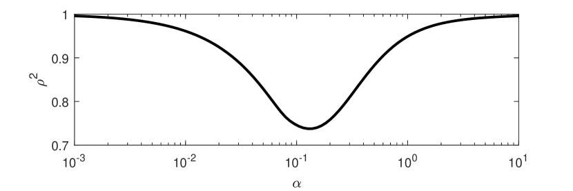
Figure 1: Plot of $\rho_{\star}^{2}(\alpha)$ under the assumptions $A\in\mathcal{M}_{\mu}$, $B\in\mathcal{C}_{\beta}\cap\mathcal{L}_{L}$, and $C\in\mathcal{C}_{\beta_{C}}$ with $\mu=1$, $\beta=0.01$, $L=5$, and $\beta_{C}=9$. The optimal parameters are $\alpha_{\star}\approx 0.131$ and $\theta_{\star}\approx 1.644$, and they produce the optimal contraction factor $\rho^{2}_{\star}\approx 0.737$. We used Matlab’s fminunc for the minimization.

Again, for simplicity of exposition, we limit the generality and consider the operator classes $\mathcal{Q}_{1}=\mathcal{M}_{\mu}$, $\mathcal{Q}_{2}=\mathcal{C}_{\beta}\cap\mathcal{L}_{L}$, and $\mathcal{Q}_{3}=\mathcal{C}_{\beta_{C}}$, as in Section 3.1.2. For $\beta\in(0,\infty)$ and $L\in(0,\infty)$, the intersection $\mathcal{C}_{\beta}\cap\mathcal{L}_{L}$ is non-degenerate. So strong duality holds by Theorem 3.4, and we use the dual OSPEP (43) to write

subject toλAμ,λBβ,λBL,λCβ≥0S(ρ2,λAμ,λBβ,λBL,λCβ,θ,α)⪰0),subscriptsuperscript𝜌2⋆𝛼𝜃fragments subject tofragmentsλ𝐴𝜇,λ𝐵𝛽,λ𝐵𝐿,λ𝐶𝛽0missing-subexpressionfragmentsS(ρ2,λ𝐴𝜇,λ𝐵𝛽,λ𝐵𝐿,λ𝐶𝛽,θ,α)succeeds-or-equals0\displaystyle\rho^{2}_{\star}(\alpha,\theta)=\left(\begin{tabular}[]{ll}$\displaystyle\operatorname*{minimize}$&$\rho^{2}$\\ subject to&$\lambda^{A}_{\mu},\lambda^{B}_{\beta},\lambda^{B}_{L},\lambda^{C}_{\beta}\geq 0$\\ &$S(\rho^{2},\lambda^{A}_{\mu},\lambda^{B}_{\beta},\lambda^{B}_{L},\lambda^{C}_{\beta},\theta,\alpha)\succeq 0$\end{tabular}\right),

minimizeρ2minimizeρ2

where $\rho^{2}$, $\lambda^{A}_{\mu}$, $\lambda^{B}_{\beta}$, $\lambda^{B}_{L}$, and $\lambda^{C}_{\beta}$ are the optimization variables and $S$ is as in (44). Note that

$$S(\rho^{2},\lambda^{A}_{\mu},\lambda^{B}_{\beta},\lambda^{B}_{L},\lambda^{C}_{\beta},\theta,\alpha)$$

$$\quad=\begin{pmatrix}\rho^{2}+\frac{\lambda^{B}_{\beta}\beta}{\alpha}+\lambda^{B}_{L}-1&\frac{\lambda^{A}_{\mu}}{2}&-\lambda^{B}_{\beta}(\frac{1}{2}+\frac{\beta}{\alpha})-\lambda^{B}_{L}&0\\ \frac{\lambda^{A}_{\mu}}{2}&\lambda^{A}_{\mu}(1+\alpha\mu)&-\lambda^{A}_{\mu}&\frac{\lambda^{A}_{\mu}}{2}\\ -\lambda^{B}_{\beta}(\frac{1}{2}+\frac{\beta}{\alpha})-\lambda^{B}_{L}&-\lambda^{A}_{\mu}&\lambda^{B}_{\beta}(\frac{\beta}{\alpha}-1)+\lambda^{B}_{L}(1-\alpha^{2}L^{2})&-\frac{\lambda^{C}_{\beta}}{2}\\ 0&\frac{\lambda^{A}_{\mu}}{2}&-\frac{\lambda^{C}_{\beta}}{2}&\frac{\lambda^{C}_{\beta}\beta_{C}}{\alpha}\end{pmatrix}-\begin{pmatrix}1\\ \theta\\ -\theta\\ 0\end{pmatrix}\begin{pmatrix}1\\ \theta\\ -\theta\\ 0\end{pmatrix}^{T}$$

is the Schur complement of

$$\tilde{S}(\rho^{2},\lambda^{A}_{\mu},\lambda^{B}_{\beta},\lambda^{B}_{L},\lambda^{C}_{\beta},\theta,\alpha)$$

$$\quad=\begin{pmatrix}\rho^{2}+\frac{\lambda^{B}_{\beta}\beta}{\alpha}+\lambda^{B}_{L}-1&\frac{\lambda^{A}_{\mu}}{2}&-\lambda^{B}_{\beta}(\frac{1}{2}+\frac{\beta}{\alpha})-\lambda^{B}_{L}&0&1\\ \frac{\lambda^{A}_{\mu}}{2}&\lambda^{A}_{\mu}(1+\alpha\mu)&-\lambda^{A}_{\mu}&\frac{\lambda^{A}_{\mu}}{2}&\theta\\ -\lambda^{B}_{\beta}(\frac{1}{2}+\frac{\beta}{\alpha})-\lambda^{B}_{L}&-\lambda^{A}_{\mu}&\lambda^{B}_{\beta}(\frac{\beta}{\alpha}-1)+\lambda^{B}_{L}(1-\alpha^{2}L^{2})&-\frac{\lambda^{C}_{\beta}}{2}&-\theta\\ 0&\frac{\lambda^{A}_{\mu}}{2}&-\frac{\lambda^{C}_{\beta}}{2}&\frac{\lambda^{C}_{\beta}\beta_{C}}{\alpha}&0\\ 1&\theta&-\theta&0&1\end{pmatrix}\in\mathbb{R}^{5\times 5}.$$

Therefore $S\succeq 0$ if and only if $\tilde{S}\succeq 0$. We use $\tilde{S}$ as it depends on $\theta$ linearly. Define $\rho^{2}_{\star}(\alpha)=\inf_{\theta\in(0,2)}\rho^{2}_{\star}(\alpha,\theta)$. We evaluate $\rho^{2}_{\star}(\alpha)$ by solving the SDP

subject toλAμ,λBβ,λBL,λCβ≥0S~(ρ2,λAμ,λBβ,λBL,λCβ,θ,α)⪰0),subscriptsuperscript𝜌2⋆𝛼fragments subject tofragmentsλ𝐴𝜇,λ𝐵𝛽,λ𝐵𝐿,λ𝐶𝛽0missing-subexpressionfragments~𝑆(ρ2,λ𝐴𝜇,λ𝐵𝛽,λ𝐵𝐿,λ𝐶𝛽,θ,α)succeeds-or-equals0\displaystyle\rho^{2}_{\star}(\alpha)=\left(\begin{tabular}[]{ll}$\displaystyle\operatorname*{minimize}$&$\rho^{2}$\\ subject to&$\lambda^{A}_{\mu},\lambda^{B}_{\beta},\lambda^{B}_{L},\lambda^{C}_{\beta}\geq 0$\\ &$\tilde{S}(\rho^{2},\lambda^{A}_{\mu},\lambda^{B}_{\beta},\lambda^{B}_{L},\lambda^{C}_{\beta},\theta,\alpha)\succeq 0$\end{tabular}\right),

minimizeρ2minimizeρ2

where $\rho^{2}$, $\lambda^{A}_{\mu}$, $\lambda^{B}_{\beta}$, $\lambda^{B}_{L}$, $\lambda^{C}_{\beta}$, and $\theta$ are the optimization variables.

It remains to solve

$$\rho_{\star}^{2}=\inf_{\alpha>0}\rho_{\star}^{2}(\alpha).$$

The function $\rho^{2}_{\star}(\alpha)$ is non-convex in $\alpha$, and it does not seem possible to compute $\rho_{\star}^{2}$ with a single SDP. However, $\rho^{2}(\alpha)$ seems to be continuous and unimodal for a wide range of operator classes and parameter choices. Continuity is not surprising. We do not know whether or why $\rho^{2}_{\star}(\alpha)$ is always unimodal.

To minimize the apparently continuous univariate unimodal function, we use Matlab’s derivative free optimization (DFO) solver fminunc. We provide a routine that evaluates $\rho^{2}_{\star}(\alpha)$ by solving an SDP, and the DFO solver calls it to evaluate $\rho^{2}_{\star}(\alpha)$ at various values of $\alpha$. Figure 1 shows an example of the function $\rho^{2}_{\star}(\alpha)$, and its minimizer was approximated with this approach. In Figure 2, we plot $\rho_{\star}^{2}(\alpha)$ under several assumptions. In all cases, $\rho_{\star}^{2}(\alpha)$ is continuous and unimodal.

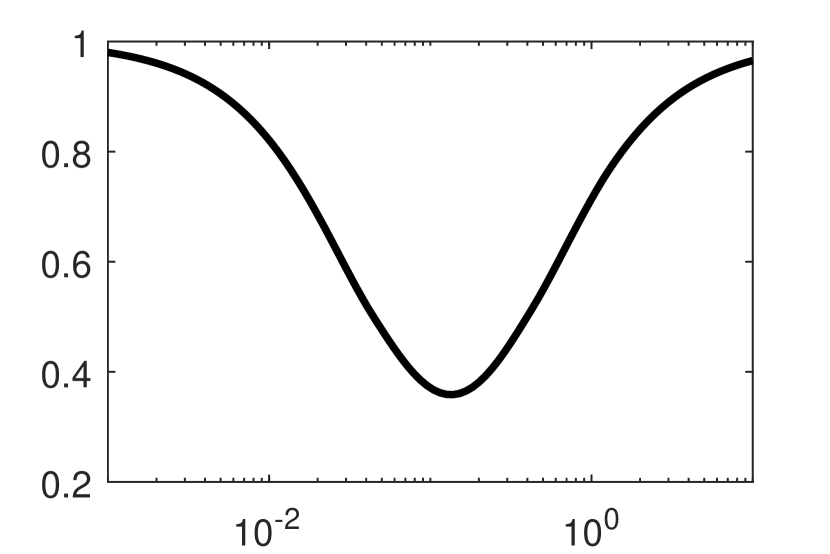
(a) $\mu_{A}=1,\beta_{A}=0.07,$
$\mu_{B}=4,\beta_{B}=0.02,\beta_{C}=9,$
$\alpha_{\star}\approx 0.13,\theta_{\star}\approx 1.57,\rho^{2}_{\star}\approx 0.36$

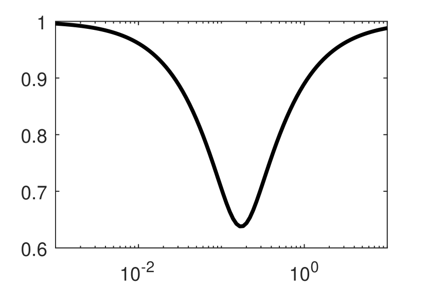
(b) $\mu_{A}=1,\beta_{B}=0.03,C=0,$
$\alpha_{\star}\approx 0.17,\theta_{\star}\approx 1.65,\rho^{2}_{\star}\approx 0.64$

(c) $\beta_{A}=0.03,\mu_{B}=1,C=0,$
$\alpha_{\star}\approx 0.17,\theta_{\star}\approx 1.65,\rho^{2}_{\star}\approx 0.64$

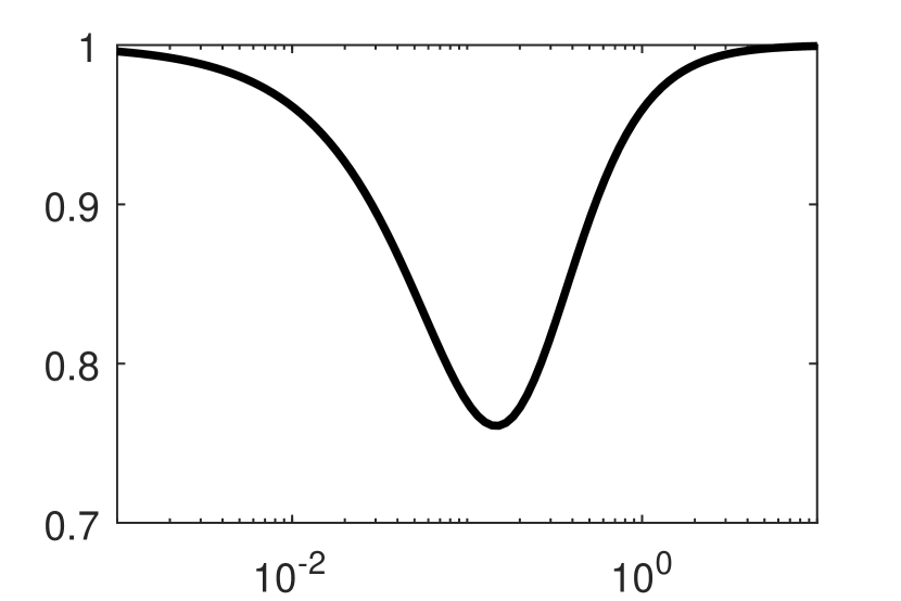
(d) $\mu_{A}=1,L_{B}=4,C=0,$
$\alpha_{\star}\approx 0.15,\theta_{\star}\approx 1.59,\rho^{2}_{\star}\approx 0.76$

(e) $L_{A}=4,\mu_{B}=1,C=0,$
$\alpha_{\star}\approx 0.15,\theta_{\star}\approx 1.59,\rho^{2}_{\star}\approx 0.76$

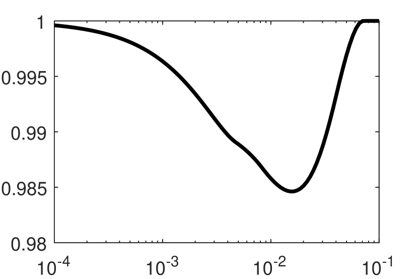
(f) $A=0,\mu_{B}=1,\beta_{B}=0.1$
$L_{C}=8,\alpha_{\star}\approx 0.016,\theta_{\star}\approx 1$
$\rho^{2}_{\star}\approx 0.98$

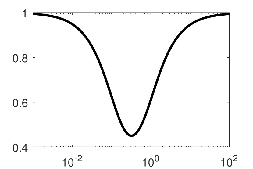
(g) $\mu_{A}=1,\beta_{A}=0.07,L_{A}=7,$
$\mu_{B}=0.03,\beta_{B}=0.02,L_{A}=2,$
$\mu_{C}=0.01,\beta_{C}=9,L_{C}=0.05,$
$\alpha_{\star}\approx 0.32,\theta_{\star}\approx 1.98,\rho^{2}_{\star}\approx 0.45$

(h) $A=0,\mu_{B}=1,\beta_{C}=0.1,$
$\alpha_{\star}\approx 0.2,\theta_{\star}\approx 1,\rho^{2}_{\star}\approx 0.69$

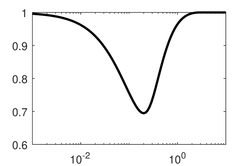
(i) $\mu_{A}=1,B=0,\beta_{C}=0.1,$
$\alpha_{\star}\approx 0.2,\theta_{\star}\approx 1,\rho^{2}_{\star}\approx 0.69$

Figure 2: Plots of $\rho_{\star}^{2}(\alpha)$ under various assumptions. The plots are unimodal in all cases. All operator classes are subsets of $\mathcal{M}$, and only the parameters used in the intersection are specified. For example, subfigure (e) uses the classes $Q_{1}=\mathcal{M}\cap\mathcal{L}_{L_{A}}$, $Q_{2}=\mathcal{M}_{\mu_{B}}$, and $Q_{3}=\{0\}$.

6 Conclusion

In this work, we presented the OSPEP methodology, proved its tightness, and demonstrated its value by presenting two applications of it. The first application was to prove tight analytic contraction factors for DRS and the second was to provide a method for automatic optimal parameter selection.

Code

With this paper, we release the following code: Matlab script implementing OSPEP for FBS, DRS, and DYS; Matlab script used to plot the figures of Section 5; and Mathematica script to help readers verify the algebra of Section SM3. The code uses YALMIP [48] and Mosek [52] and is available at
https://github.com/AdrienTaylor/OperatorSplittingPerformanceEstimation.

For splitting methods applied to convex functions, one can use the Matlab toolbox PESTO [72], available at
https://github.com/AdrienTaylor/Performance-Estimation-Toolbox.

Appendix

SM1 Full primal OSPEP

We state the full primal OSPEP with the operator classes $\mathcal{Q}_{1}=\mathcal{M}_{\mu_{A}}\cap\mathcal{C}_{\beta_{A}}\cap\mathcal{L}_{L_{A}}$, $\mathcal{Q}_{2}=\mathcal{M}_{\mu_{B}}\cap\mathcal{C}_{\beta_{B}}\cap\mathcal{L}_{L_{B}}$, and $\mathcal{Q}_{3}=\mathcal{M}_{\mu_{C}}\cap\mathcal{C}_{\beta_{C}}\cap\mathcal{L}_{L_{C}}$. The primal OSPEP with fewer assumptions will be of an analogous form with fewer constraints.

where $G\in\mathbb{S}^{4}_{+}$ is the optimization variable and

$$M_{I}=\begin{pmatrix}1&0&0&0\\ 0&0&0&0\\ 0&0&0&0\\ 0&0&0&0\end{pmatrix},\qquad M_{O}=\begin{pmatrix}1&\theta&-\theta&0\\ \theta&\theta^{2}&-\theta^{2}&0\\ -\theta&-\theta^{2}&\theta^{2}&0\\ 0&0&0&0\end{pmatrix}$$

$$M^{A}_{\mu}=\begin{pmatrix}0&-\frac{1}{2}&0&0\\ -\frac{1}{2}&-\alpha\mu_{A}-1&1&-\frac{1}{2}\\ 0&1&0&0\\ 0&-\frac{1}{2}&0&0\\ \end{pmatrix},\qquad M^{A}_{\beta}=\begin{pmatrix}-\tfrac{\beta_{A}}{\alpha}&-\tfrac{\beta_{A}}{\alpha}-\tfrac{1}{2}&\tfrac{2\beta_{A}}{\alpha}&-\tfrac{\beta_{A}}{\alpha}\\ -\tfrac{\beta_{A}}{\alpha}-\tfrac{1}{2}&-\tfrac{\beta_{A}}{\alpha}-1&\tfrac{2\beta_{A}}{\alpha}+1&-\tfrac{\beta_{A}}{\alpha}-\tfrac{1}{2}\\ \tfrac{2\beta_{A}}{\alpha}&\tfrac{2\beta_{A}}{\alpha}+1&-\tfrac{4\beta_{A}}{\alpha}&\tfrac{2\beta_{A}}{\alpha}\\ -\tfrac{\beta_{A}}{\alpha}&-\tfrac{\beta_{A}}{\alpha}-\tfrac{1}{2}&\tfrac{2\beta_{A}}{\alpha}&-\tfrac{\beta_{A}}{\alpha}\end{pmatrix},$$

$$M^{A}_{L}=\begin{pmatrix}-1&-1&2&-1\\ -1&\alpha^{2}L_{A}^{2}-1&2&-1\\ 2&2&-4&2\\ -1&-1&2&-1\end{pmatrix},\qquad M^{B}_{\mu}=\begin{pmatrix}0&0&\tfrac{1}{2}&0\\ 0&0&0&0\\ \tfrac{1}{2}&0&-\alpha\mu_{B}-1&0\\ 0&0&0&0\end{pmatrix},$$

$$M^{B}_{\beta}=\begin{pmatrix}-\tfrac{\beta_{B}}{\alpha}&0&\tfrac{\beta_{B}}{\alpha}+\tfrac{1}{2}&0\\ 0&0&0&0\\ \tfrac{\beta_{B}}{\alpha}+\tfrac{1}{2}&0&-\tfrac{\beta_{B}}{\alpha}-1&0\\ 0&0&0&0\end{pmatrix},\qquad M^{B}_{L}=\begin{pmatrix}-1&0&1&0\\ 0&0&0&0\\ 1&0&\alpha^{2}L_{B}^{2}-1&0\\ 0&0&0&0\end{pmatrix},$$

$$M^{C}_{\mu}=\begin{pmatrix}0&0&0&0\\ 0&0&0&0\\ 0&0&-\alpha\mu_{C}&\tfrac{1}{2}\\ 0&0&\tfrac{1}{2}&0\end{pmatrix},\qquad M^{C}_{\beta}=\begin{pmatrix}0&0&0&0\\ 0&0&0&0\\ 0&0&0&\tfrac{1}{2}\\ 0&0&\tfrac{1}{2}&-\tfrac{\beta_{C}}{\alpha}\end{pmatrix},\qquad M^{C}_{L}=\begin{pmatrix}0&0&0&0\\ 0&0&0&0\\ 0&0&\alpha^{2}L_{C}^{2}&0\\ 0&0&0&-1\end{pmatrix}.$$

The objective $\operatorname*{Tr}(M_{O}G)$ corresponds to $\|z-\theta(z_{B}-z_{A})-z^{\prime}+\theta(z_{B}^{\prime}-z_{A}^{\prime})\|^{2}$. The equality constraint $\operatorname*{Tr}(M_{I}G)=1$ corresponds to $\|z-z^{\prime}\|^{2}=1$. The other $9$ inequality constraints correspond to the three assumptions on the three operators. In particular, $\operatorname*{Tr}(M_{\mu}^{A}G)\geq 0$, $\operatorname*{Tr}(M_{\beta}^{A}G)\geq 0$, and $\operatorname*{Tr}(M_{L}^{A}G)\geq 0$ respectively correspond to the $\mu$-strong monotonicity, $\beta$-cocoercivity, and $L$-Lipschitz continuity assumptions on $A$ respectively. The assumptions on $B$ and $C$ have analogous correspondences.

SM2 Full dual OSPEP

We state the full dual OSPEP with the same operator classes as in Section SM1. The dual OSPEP with fewer assumptions will be of an analogous form with fewer $\lambda$-variables.

$$\operatorname*{minimize}{}$$

subject to

where $\rho^{2},\lambda^{A}_{\mu},\lambda^{A}_{\beta},\lambda^{A}_{L},\lambda^{B}_{\mu},\lambda^{B}_{\beta},\lambda^{B}_{L},\lambda^{C}_{\mu},\lambda^{C}_{\beta},\lambda^{C}_{L}\in\mathbb{R}$ are the optimization variables and

$$S(\rho^{2},\lambda^{A}_{\mu},\lambda^{A}_{\beta},\lambda^{A}_{L},\lambda^{B}_{\mu},\lambda^{B}_{\beta},\lambda^{B}_{L},\lambda^{C}_{\mu},\lambda^{C}_{\beta},\lambda^{C}_{L},\theta,\alpha)=\rho^{2}M_{I}-M_{O} -\lambda_{\mu}^{A}M_{\mu}^{A}-\lambda_{\beta}^{A}M_{\beta}^{A}-\lambda_{L}^{A}M_{L}^{A}$$

$$-\lambda_{\mu}^{B}M_{\mu}^{B}-\lambda_{\beta}^{B}M_{\beta}^{B}-\lambda_{L}^{B}M_{L}^{B}$$

$$-\lambda_{\mu}^{C}M_{\mu}^{C}-\lambda_{\beta}^{C}M_{\beta}^{C}-\lambda_{L}^{C}M_{L}^{C}$$

is symmetric. The matrix can also explicitly be written as

$$S(\rho^{2},\lambda^{A}_{\mu},\lambda^{A}_{\beta},\lambda^{A}_{L},\lambda^{B}_{\mu},\lambda^{B}_{\beta},\lambda^{B}_{L},\lambda^{C}_{\mu},\lambda^{C}_{\beta},\lambda^{C}_{L},\theta,\alpha)=\begin{pmatrix}S_{1,1}&S_{2,1}&S_{3,1}&S_{4,1}\\ S_{2,1}&S_{2,2}&S_{3,2}&S_{4,2}\\ S_{3,1}&S_{3,2}&S_{3,3}&S_{4,3}\\ S_{4,1}&S_{4,2}&S_{4,3}&S_{4,4}\end{pmatrix}$$

with

$$S_{1,1} =\rho^{2}-1+\tfrac{\beta_{A}}{\alpha}\lambda_{\beta}^{A}+\tfrac{\beta_{B}}{\alpha}\lambda_{\beta}^{B}+\lambda_{L}^{A}+\lambda_{L}^{B},$$

$$S_{2,1} =\tfrac{1}{2}(2\tfrac{\beta_{A}}{\alpha}\lambda_{\beta}^{A}-2\theta+\lambda_{\beta}^{A}+2\lambda_{L}^{A}+\lambda_{\mu}^{A}),$$

$$S_{3,1} =-2\tfrac{\beta_{A}}{\alpha}\lambda_{\beta}^{A}-\tfrac{\beta_{B}}{\alpha}\lambda_{\beta}^{B}+\theta-2\lambda_{L}^{A}-\tfrac{\lambda_{\beta}^{B}}{2}-\lambda_{L}^{B}-\tfrac{\lambda_{\mu}^{B}}{2},$$

$$S_{4,1} =\tfrac{\beta_{A}}{\alpha}\lambda_{\beta}^{A}+\lambda_{L}^{A},$$

$$S_{2,2} =\tfrac{\beta_{A}}{\alpha}\lambda_{\beta}^{A}-\theta^{2}+\lambda_{\beta}^{A}+\lambda_{L}^{A}+\lambda_{\mu}^{A}\alpha\mu_{A}+\lambda_{\mu}^{A}-\lambda_{L}^{A}\alpha^{2}L_{A}^{2},$$

$$S_{3,2} =-(2\tfrac{\beta_{A}}{\alpha}+1)\lambda_{\beta}^{A}+\theta^{2}-2\lambda_{L}^{A}-\lambda_{\mu}^{A},$$

$$S_{4,2} =\tfrac{1}{2}(2\tfrac{\beta_{A}}{\alpha}\lambda_{\beta}^{A}+\lambda_{\beta}^{A}+2\lambda_{L}^{A}+\lambda_{\mu}^{A}),$$

$$S_{3,3} =4\tfrac{\beta_{A}}{\alpha}\lambda_{\beta}^{A}+\tfrac{\beta_{B}}{\alpha}\lambda_{\beta}^{B}-\theta^{2}+4\lambda_{L}^{A}+\lambda_{\beta}^{B}+\lambda_{L}^{B}+\lambda_{\mu}^{B}\alpha\mu_{B}+\lambda_{\mu}^{B}+\lambda_{\mu}^{C}\alpha\mu_{C}-\lambda_{L}^{B}\alpha^{2}L_{B}^{2}-\lambda_{L}^{C}\alpha^{2}L_{C}^{2},$$

$$S_{4,3} =\tfrac{1}{2}(-4\tfrac{\beta_{A}}{\alpha}\lambda_{\beta}^{A}-4\lambda_{L}^{A}-\lambda_{\beta}^{C}-\lambda_{\mu}^{C}),$$

$$S_{4,4} =\tfrac{\beta_{A}}{\alpha}\lambda_{\beta}^{A}+\tfrac{\beta_{C}}{\alpha}\lambda_{\beta}^{C}+\lambda_{L}^{A}+\lambda_{L}^{C}.$$

SM3 Proofs of results in Section 4

We now prove Theorems 4.1 and 4.4. The approach is to provide an upper bound and a lower bound for each case (5 cases for Theorem 4.1 and 3 cases for Theorem 4.4). Since the upper and lower bounds match, weak duality tells us that the bounds are optimal, i.e., the contraction factors are tight.

In the language of the SDPs, the upper and lower bounds correspond to primal and dual feasible points, and their optimality is certified since they match ($0$ duality gap). Note that the strong duality result of Theorem 3.4 guarantees the existence of lower bounds matching the optimal upper bounds. Here, we explicitly provide lower bounds to certify the upper bounds are indeed optimal.

The proofs rely on inequalities that we assert by saying “It is possible to verify that ….” Whenever we do so, we provide a rigorous (and arduous) verification separately in Section SM4. We make this separation because the verifications are purely algebraic and do not illuminate the main proof. As an alternative means of verification, we provide code that uses symbolic manipulation to verify the inequalities.

SM3.1 Proof of Theorem 4.1

Define

$$R_{\mathrm{(a)}} =\left\{(\mu,\beta,\theta)\,\Big{|}\,\mu\beta-\mu+\beta<0,\,\theta\leq 2\tfrac{(\beta+1)(\mu-\beta-\mu\beta)}{\mu+\mu\beta-\beta-\beta^{2}-2\mu\beta^{2}},\,\mu>0,\,\beta>0,\,\theta\in(0,2)\right\}$$

$$R_{\mathrm{(b)}} =\left\{(\mu,\beta,\theta)\,\Big{|}\,\mu\beta-\mu-\beta>0,\,\theta\leq 2\tfrac{\mu^{2}+\beta^{2}+\mu\beta+\mu+\beta-\mu^{2}\beta^{2}}{\mu^{2}+\beta^{2}+\mu^{2}\beta+\mu\beta^{2}+\mu+\beta-2\mu^{2}\beta^{2}},\,\mu>0,\,\beta>0,\,\theta\in(0,2)\right\}$$

$$R_{\mathrm{(c)}} =\left\{(\mu,\beta,\theta)\,\Big{|}\,\theta\geq 2\tfrac{\mu\beta+\mu+\beta}{2\mu\beta+\mu+\beta},\,\mu>0,\,\beta>0,\,\theta\in(0,2)\right\}$$

$$R_{\mathrm{(d)}} =\left\{(\mu,\beta,\theta)\,\Big{|}\,\mu\beta+\mu-\beta<0,\,\theta\leq 2\tfrac{(\mu+1)(\beta-\mu-\mu\beta)}{\beta+\mu\beta-\mu-\mu^{2}-2\mu^{2}\beta},\,\mu>0,\,\beta>0,\,\theta\in(0,2)\right\}$$

$$R_{\mathrm{(e)}} =\left\{(\mu,\beta,\theta)\,\Big{|}\,\mu>0,\,\beta>0,\,\theta\in(0,2)\right\}\backslash R_{\mathrm{(a)}}\backslash R_{\mathrm{(b)}}\backslash R_{\mathrm{(c)}}\backslash R_{\mathrm{(d)}}$$

which correspond to the 5 cases of Theorem 4.1.

SM3.1.1 Upper bounds

By weak duality between the primal and dual OSPEP, $\rho$ is a valid contraction factor if there exists $\rho$, $\lambda^{A}_{\mu}\geq 0$, and $\lambda_{\beta}^{B}\geq 0$ such that

$$S=\begin{pmatrix}\rho^{2}+\beta\lambda_{\beta}^{B}-1&-\theta+\frac{\lambda^{A}_{\mu}}{2}&\theta-(\frac{1}{2}+\beta)\lambda_{\beta}^{B}\\ -\theta+\frac{\lambda^{A}_{\mu}}{2}&-\theta^{2}+(1+\mu)\lambda^{A}_{\mu}&\theta^{2}-\lambda^{A}_{\mu}\\ \theta-(\frac{1}{2}+\beta)\lambda_{\beta}^{B}&\theta^{2}-\lambda^{A}_{\mu}&-\theta^{2}+(1+\beta)\lambda_{\beta}^{B}\end{pmatrix}\succeq 0.$$

For each of the 5 cases, we establish an upper bound by providing values for $\rho$, $\lambda^{A}_{\mu}\geq 0$, and $\lambda_{\beta}^{B}\geq 0$ such that $S\succeq 0$. We establish $S\succeq 0$ with a sum-of-squares factorization

(45) $$\mathrm{Tr}(SG(z,z_{A},z_{B}))=K_{1}{\lVert m_{1}z_{A}+m_{2}z_{B}+m_{3}z\rVert^{2}}+K_{2}{\lVert m_{4}z_{B}+m_{5}z\rVert^{2}},$$

for some $m_{1},m_{2},m_{3},m_{4},m_{5}\in\mathbb{R}$ and $K_{1},K_{2}\geq 0$, where

(46) $$G(z,z_{A},z_{B})=\begin{pmatrix}\|z\|^{2}&\langle z,z_{A}\rangle&\langle z,z_{B}\rangle\\ \langle z,z_{A}\rangle&\|z_{A}\|^{2}&\langle z_{A},z_{B}\rangle\\ \langle z,z_{B}\rangle&\langle z_{A},z_{B}\rangle&\|z_{B}\|^{2}\\ \end{pmatrix}\in\mathbb{S}^{3}_{+}$$

for $z,z_{A},z_{B}\in\mathcal{H}$. By arguments similar to that of Lemma 3.1, $G(z,z_{A},z_{B})\in\mathbb{S}^{3}_{+}$ can be any $3\times 3$ positive semidefinite matrix. Therefore

$$\mathrm{Tr}(SG(z,z_{A},z_{B}))\geq 0,\,\forall z,z_{A},z_{A}\in\mathcal{H}\quad\Leftrightarrow\quad\mathrm{Tr}(SM)\geq 0,\,\forall M\succeq 0\quad\Leftrightarrow\quad S\succeq 0,$$

i.e., the sum-of-squares factorization proves $S\succeq 0$. (We only need 2 terms in the sum-of-squares factorization, because it turns out that the optimal $S$ has rank at most $2$.)

Case (a)

When $(\mu,\beta,\theta)\in R_{\mathrm{(a)}}$, we use

$$\rho^{2}=\left(1-\theta\tfrac{\beta}{\beta+1}\right)^{2},\quad\lambda^{A}_{\mu}=2\theta\tfrac{1+\beta}{1-\beta}\left(1-\theta\tfrac{\beta}{\beta+1}\right),\quad\lambda_{\beta}^{B}=2\theta\left(1-\theta\tfrac{\beta}{\beta+1}\right).$$

This gives us the sum-of-square factorization (45) with

$$m_{1}=-1,\quad m_{2}=\tfrac{(2-\theta)(\beta+1)}{(2-\theta)(\beta+1)+2\mu(1+\beta-\theta\beta)},\quad m_{3}=-\tfrac{(2-\theta)\beta}{(2-\theta)(\beta+1)+2\mu(1+\beta-\theta\beta)},$$

$$m_{4}=-\tfrac{\beta+1}{\beta},m_{5}=1,\quad K_{1}=\theta\tfrac{(2-\theta)(\beta+1)+2\mu(1+\beta-\theta\beta)}{1-\beta},\quad K_{2}=2\beta^{2}\theta\tfrac{1+\beta-\theta\beta}{(1-\beta)(\beta+1)^{2}}\tfrac{(\beta-1)\mu(2\beta(\theta-1)+\theta-2)-(2-\theta)\beta(\beta+1)}{(2-\theta)(\beta+1)+2\mu(1+\beta-\theta\beta)}.$$

It is possible to verify that there is no division by $0$ in the definitions and that $\lambda^{A}_{\mu},\lambda_{\beta}^{B},K_{1},K_{2}\geq 0$ when $(\mu,\beta,\theta)\in R_{\mathrm{(a)}}$.

Case (b)

When $(\mu,\beta,\theta)\in R_{\mathrm{(b)}}$, we use

$$\rho^{2}=\left(1-\theta\tfrac{1+\mu\beta}{(\mu+1)(\beta+1)}\right)^{2},\quad\lambda^{A}_{\mu}=2\theta\tfrac{\beta+1}{\beta-1}\left(1-\theta\tfrac{1+\mu\beta}{(\mu+1)(\beta+1)}\right),\quad\lambda_{\beta}^{B}=2\theta\tfrac{\mu-1}{\mu+1}\left(1-\theta\tfrac{1+\mu\beta}{(\mu+1)(\beta+1)}\right).$$

This gives us the sum-of-square factorization (45) with

$$m_{1}=-1,\quad m_{2}=\tfrac{2}{\mu+1}-\tfrac{(2-\theta)(\beta+1)}{(2-\theta)(\beta+1)+2\mu(1+\beta-\theta\beta)},\quad m_{3}=-\tfrac{1}{\mu+1}+\tfrac{(2-\theta)\beta}{(2-\theta)(\beta+1)+2\mu(1+\beta-\theta\beta)},$$

$$m_{4}=-\tfrac{\beta+1}{\beta},\quad m_{5}=1,\quad K_{1}=\theta\tfrac{(2-\theta)(\beta+1)+2\mu(1+\beta-\theta\beta)}{\beta-1},$$

$$K_{2}=2\theta\beta^{2}\tfrac{(\beta+1)(\mu+1)-\theta(1+\mu\beta)}{(\mu+1)^{2}(\beta-1)(\beta+1)^{2}}\,\tfrac{\mu\beta^{2}(-2\theta\mu+\theta+2\mu)+\theta\beta^{2}+(\theta-2)\mu(\mu+1)+\beta\left(\theta\mu^{2}+\theta-2\mu-2\right)-2\beta^{2}}{(2-\theta)(\beta+1)+2\mu(1+\beta-\theta\beta)}.$$

It is possible to verify that there is no division by $0$ in the definitions and that $\lambda^{A}_{\mu},\lambda_{\beta}^{B},K_{1},K_{2}\geq 0$ when $(\mu,\beta,\theta)\in R_{\mathrm{(b)}}$.

Case (c)

When $(\mu,\beta,\theta)\in R_{\mathrm{(c)}}$, we use

$$\rho^{2}=(\theta-1)^{2},\quad\lambda^{A}_{\mu}=2\theta(\theta-1),\quad\lambda_{\beta}^{B}=2\theta(\theta-1)$$

This gives us the sum-of-square factorization (45) with

$$m_{1}=-1,\quad m_{2}=-\tfrac{2-\theta}{2(\theta-1)\mu+\theta-2},\quad m_{3}=\tfrac{2-\theta}{2(\theta-1)\mu+\theta-2},\quad m_{4}=-1,\quad m_{5}=1,$$

$$K_{1}=\theta(2(\theta-1)\mu+\theta-2),\quad K_{2}=2(\theta-1)\theta\tfrac{\theta\beta+\theta\mu(1+2\beta)-2(\mu+\beta+\mu\beta)}{2(\theta-1)\mu+\theta-2}.$$

It is possible to verify that there is no division by $0$ in the definitions and that $\lambda^{A}_{\mu},\lambda_{\beta}^{B},K_{1},K_{2}\geq 0$ when $(\mu,\beta,\theta)\in R_{\mathrm{(c)}}$.

Case (d)

When $(\mu,\beta,\theta)\in R_{\mathrm{(d)}}$, we use

$$\rho^{2}=\left(1-\theta\tfrac{\mu}{\mu+1}\right)^{2},\quad\lambda^{A}_{\mu}=2\theta\left(1-\theta\tfrac{\mu}{\mu+1}\right),\quad\lambda_{\beta}^{B}=2\theta\tfrac{1-\mu}{1+\mu}\left(1-\theta\tfrac{\mu}{\mu+1}\right).$$

This gives us the sum-of-square factorization (45) with

$$m_{1}=-1,\quad m_{2}=\tfrac{2-\theta}{2(\theta-1)\mu+\theta-2}+\tfrac{2}{\mu+1},\quad m_{3}=-\tfrac{\theta\mu}{(\mu+1)(2(\theta-1)\mu+\theta-2)},\quad m_{4}=-1,\quad m_{5}=1,$$

$$K_{1}=-\theta(2(\theta-1)\mu+\theta-2),\quad K_{2}=2\theta((\theta-1)\mu-1)\tfrac{-\theta(\beta-\mu^{2}(1+2\beta)-\mu(1-\beta))-2(\mu+1)(\mu\beta+\mu-\beta)}{(\mu+1)^{2}(2(\theta-1)\mu+\theta-2)}.$$

It is possible to verify that there is no division by $0$ in the definitions and that $\lambda^{A}_{\mu},\lambda_{\beta}^{B},K_{1},K_{2}\geq 0$ when $(\mu,\beta,\theta)\in R_{\mathrm{(d)}}$.

Case (e)

When $(\mu,\beta,\theta)\in R_{\mathrm{(e)}}$, we use

$$\rho^{2}=\tfrac{2-\theta}{4}{\tfrac{((2-\theta)\mu(\beta+1)+{\theta}\beta(1-\mu))\,((2-\theta)\beta({\mu}+1)+{\theta}\mu(1-\beta))}{\mu\beta(2\mu\beta(1-\theta)+(2-\theta)(\mu+\beta+1))}},\quad\lambda^{A}_{\mu}=\theta\tfrac{(2-\theta)\mu(\beta+1)+\theta\beta(1-\mu)}{\beta},$$

$$\lambda_{\beta}^{B}=\tfrac{\theta(2-\theta)}{\beta}\tfrac{(2-\theta)\mu(\beta+1)+\theta\beta(1-\mu)}{2\mu\beta(1-\theta)+(2-\theta).(\mu+\beta+1)}.$$

This gives us the sum-of-square factorization (45) with

$$m_{1}=-2\mu\tfrac{2(\theta-1)\mu\beta+\theta\beta+(\theta-2)(\mu+1)-2\beta}{\beta},\quad m_{2}=2\mu\tfrac{(\beta+1)(\theta-2)+\beta\theta}{\beta},\quad m_{3}=(\theta-2)-\mu\tfrac{(\beta+1)(\theta-2)+\beta\theta}{\beta}$$

$$m_{4}=0,\quad m_{5}=0,\quad K_{1}=\tfrac{\beta}{4\mu}\,\,\tfrac{\theta}{2\mu\beta(1-\theta)+(2-\theta)(\mu+\beta+1)},\quad K_{2}=0.$$

It is possible to verify that there is no division by $0$ in the definitions and that $\rho^{2},\lambda^{A}_{\mu},\lambda_{\beta}^{B},K_{1},K_{2}\geq 0$ when $(\mu,\beta,\theta)\in R_{\mathrm{(e)}}$.

Remark 1 (Constructing a classical proof with a dual solution).

Given $\rho^{2}$, $\lambda^{A}_{\mu}\geq 0$, and $\lambda_{\beta}^{B}\geq 0$ such that $S\succeq 0$, one can construct a classical proof establishing $\rho^{2}$ as a valid contraction factor without relying on the OSPEP methodology. With $G$ defined as in (46), we have

$$\mathrm{Tr}(SG(z,z_{A},z_{B}))=\rho^{2}{\lVert z\rVert^{2}}-{\lVert z-\theta(z_{B}-z_{A})\rVert^{2}}-\lambda^{A}_{\mu}\bigg{(}{\langle\Delta A,z_{A}\rangle}-\mu{\lVert z_{A}\rVert^{2}}\bigg{)}-\lambda_{\beta}^{B}\bigg{(}{\langle\Delta B,z_{B}\rangle}-\beta{\lVert\Delta B\rVert^{2}}\bigg{)},$$

with $\Delta A=2z_{b}-z-z_{A}$ and $\Delta B=z-z_{B}$. The sum-of-square factorization gives us

$$\rho^{2}{\lVert z\rVert^{2}}-{\lVert z-\theta(z_{B}-z_{A})\rVert^{2}}-\lambda^{A}_{\mu}\bigg{(}{\langle\Delta A,z_{A}\rangle}-\mu{\lVert z_{A}\rVert^{2}}\bigg{)}-\lambda_{\beta}^{B}\bigg{(}{\langle\Delta B,z_{B}\rangle}-\beta{\lVert\Delta B\rVert^{2}}\bigg{)}$$

$$\qquad\qquad=K_{1}{\lVert m_{1}z_{A}+m_{2}z_{B}+m_{3}z\rVert^{2}}+K_{2}{\lVert m_{4}z_{B}+m_{5}z\rVert^{2}}.$$

Reorganizing, we get

$${\lVert z-\theta(z_{B}-z_{A})\rVert^{2}} =\rho^{2}{\lVert z\rVert^{2}}-\lambda^{A}_{\mu}\bigg{(}{\langle\Delta A,z_{A}\rangle}-\mu{\lVert z_{A}\rVert^{2}}\bigg{)}-\lambda_{\beta}^{B}\bigg{(}{\langle\Delta B,z_{B}\rangle}-\beta{\lVert\Delta B\rVert^{2}}\bigg{)}$$

$$\qquad\qquad-(\text{sum of squares}).$$

Now revert the change of variables of Section 3.1 by substituting $z\mapsto z-z^{\prime}$, $z-\theta(z_{B}-z_{A})\mapsto T^{\mathrm{DRS}}(z)-T^{\mathrm{DRS}}(z^{\prime})$, $z_{B}\mapsto J_{B}z-J_{B}z^{\prime}$, and $z_{A}\mapsto J_{A}(2J_{B}z-z)-J_{A}(2J_{B}z^{\prime}-z^{\prime})$ to get a classical proof of the form

$$\|T^{\mathrm{DRS}}(z;A,B,1,\theta) -T^{\mathrm{DRS}}(z^{\prime};A,B,1,\theta)\|^{2}=\rho^{2}{\lVert z-z^{\prime}\rVert^{2}}$$

$$-\lambda^{A}_{\mu}\bigg{(}{\langle\Delta A,J_{A}(2J_{B}z-z)-J_{A}(2J_{B}z^{\prime}-z^{\prime})\rangle}-\mu{\lVert J_{A}(2J_{B}z-z)-J_{A}(2J_{B}z^{\prime}-z^{\prime})\rVert^{2}}\bigg{)}$$

$$-\lambda_{\beta}^{B}\bigg{(}{\langle\Delta B,J_{B}z-J_{B}z^{\prime}\rangle}-\beta{\lVert\Delta B\rVert^{2}}\bigg{)}$$

$$-(\text{sum of squares})$$

where now $\Delta A=2J_{B}z-z-J_{A}(2J_{B}z-z)-2J_{B}z^{\prime}+z^{\prime}+J_{A}(2J_{B}z^{\prime}-z^{\prime})$ and $\Delta B=z-J_{B}z-z^{\prime}+J_{B}z^{\prime}$. Since $A$ is $\mu$-strong monotone, we have

$${\langle\Delta A,J_{A}(2J_{B}z-z)-J_{A}(2J_{B}z^{\prime}-z^{\prime})\rangle}-\mu{\lVert J_{A}(2J_{B}z-z)-J_{A}(2J_{B}z^{\prime}-z^{\prime})\rVert^{2}}\geq 0.$$

Since $B$ is $\beta$-cocoercive, we have

$${\langle\Delta B,J_{B}z-J_{B}z^{\prime}\rangle}-\beta{\lVert\Delta B\rVert^{2}}\geq 0.$$

Since $\lambda^{A}_{\mu}\geq 0$ and $\lambda_{\beta}^{B}\geq 0$, we have a valid proof establishing

$$\|T^{\mathrm{DRS}}(z;A,B,1,\theta)-T^{\mathrm{DRS}}(z^{\prime};A,B,1,\theta)\|^{2}\leq\rho^{2}{\lVert z-z^{\prime}\rVert^{2}}.$$

SM3.1.2 Lower bounds

We now show that for the five cases, there are operators $A\in\mathcal{M}_{\mu}$ and $B\in\mathcal{C}_{\beta}$ and inputs $z_{1},z_{2}\in\mathcal{H}$ such that

$${\lVert Tz_{1}-Tz_{2}\rVert}\geq\rho{\lVert z_{1}-z_{2}\rVert},$$

where $T=I-\theta J_{B}+\theta J_{A}(2J_{B}-I)$ and $\rho$ is given by Theorem 4.1. We construct the lower bounds for $\mathbb{R}^{2}$, since the construction can be embedded into the higher dimensional space $\mathcal{H}$.

Case (a)

$A=N_{\{0\}}$, $B=\tfrac{1}{\beta}I$, and $T=\left(1-\theta\tfrac{\beta}{1+\beta}\right)I$. This construction provides the lower bound $\rho=\lvert 1-\theta\tfrac{\beta}{\beta+1}\rvert$, and it is valid when $(\mu,\beta,\theta)\in R_{\mathrm{(a)}}$. (In fact, it is always valid.)

Case (b)

$A=\mu I$, $B=\tfrac{1}{\beta}I$, and $T=\left(1-\theta\tfrac{1+\beta\mu}{(\beta+1)(\mu+1)}\right)I$. This construction provides the lower bound $\rho=\lvert 1-\theta\tfrac{1+\mu\beta}{(\mu+1)(\beta+1)}\rvert$, and it is valid when $(\mu,\beta,\theta)\in R_{\mathrm{(b)}}$. (In fact, it is always valid.)

Case (c)

$A=N_{\{0\}}$, $B=0$, and $T=(1-\theta)I$. This construction provides the lower bound $\rho=\lvert 1-\theta\rvert$, and it is valid when $(\mu,\beta,\theta)\in R_{\mathrm{(c)}}$. (In fact, it is always valid.)

Case (d)

$A=\mu I$, $B=0$, and $T=\left(1-\theta\tfrac{\mu}{\mu+1}\right)I$. This construction provides the lower bound $\rho=\lvert 1-\theta\tfrac{\mu}{\mu+1}\rvert$, and it is valid when $(\mu,\beta,\theta)\in R_{\mathrm{(d)}}$. (In fact, it is always valid.)

Case (e)

Define

$$K=\tfrac{((2-\theta)\mu(\mu+1)+\beta(\mu-1)(2-\theta+2\mu(1-\theta)))\,((2-\theta)\mu+\beta(2(1-\theta)\mu-\theta+2))}{\beta^{2}(\theta-2)\mu(2\beta(\theta-2)-\theta-2)+\beta^{2}(2\beta+1)(\theta-2)^{2}+(2\beta-1)\mu^{3}(2\beta(\theta-1)+\theta-2)^{2}-(2\beta-1)\mu^{2}(2\beta-\theta+2)(2\beta(\theta-1)+\theta-2)}.$$

It is possible to verify that there is no division by $0$ in the definition of $K$ and that $0<K<1/\beta^{2}$ when $(\mu,\beta,\theta)\in R_{\mathrm{(e)}}$. Let

$$A=\begin{pmatrix}\mu&-a\\ a&\mu\\ \end{pmatrix},\qquad B=\begin{pmatrix}\beta K&-\sqrt{K-K^{2}\beta^{2}}\\ \sqrt{K-K^{2}\beta^{2}}&\beta K\end{pmatrix},$$

where

$$a=\tfrac{2\theta\mu+\theta-2\beta\theta K\mu-\theta K+2K\mu+2K-2\mu-2+\sqrt{4(\theta-2)^{2}(\mu+1)^{2}\left(K-\beta^{2}K^{2}\right)+((\theta-2)(K-1)-2\mu(\theta-\beta\theta K+K-1))^{2}}}{2(\theta-2)\sqrt{K-\beta^{2}K^{2}}}.$$

Since $\tfrac{1}{2}(A+A^{T})$ has two eigenvalues equal to $\mu$ and $\tfrac{1}{2}(B^{-T}+B^{-1})$ has two eigenvalues equal to $\beta$, we have $A\in\mathcal{M}_{\mu}$ and $B\in\mathcal{C}_{\beta}$. Then

$$T=\begin{pmatrix}T_{1}&-T_{2}\\ T_{2}&T_{1}\\ \end{pmatrix}$$

with

$$\begin{aligned} T_{1}&=\tfrac{-\theta\left(a^{2}(\beta K+1)+(\mu+1)(K(\beta\mu+\beta+1)+\mu)\right)+\left(a^{2}+(\mu+1)^{2}\right)(2\beta K+K+1)-2a\theta\sqrt{K-\beta^{2}K^{2}}}{\left(a^{2}+(\mu+1)^{2}\right)(2\beta K+K+1)},\\ T_{2}&=\tfrac{\theta\left(a^{2}\sqrt{K-\beta^{2}K^{2}}+a(K-1)+\left(\mu^{2}-1\right)\sqrt{K-\beta^{2}K^{2}}\right)}{\left(a^{2}+(\mu+1)^{2}\right)(2\beta K+K+1)}\end{aligned},$$

and

$$T^{T}T=\begin{pmatrix}T_{1}^{2}+T_{2}^{2}&0\\ 0&T_{1}^{2}+T_{2}^{2}\end{pmatrix}.$$

So this construction provides the lower bound $\rho^{2}=T_{1}^{2}+T_{2}^{2}$. Under the assumption $\theta<2\tfrac{\beta\mu+\beta+\mu}{2\beta\mu+\beta+\mu}$ (i.e., when $(\mu,\beta,\theta)\notin R_{\mathrm{(c)}}$), the lower bound simplifies to

$$\rho=\tfrac{\sqrt{2-\theta}}{2}\sqrt{\tfrac{((2-\theta)\mu(\beta+1)-{\theta\beta}(\mu-1))\,((2-\theta)\beta(\mu+1)-{\theta}\mu(\beta-1))}{\mu\beta(2\mu\beta(1-\theta)+(2-\theta)(\mu+\beta+1))}},$$

and it is valid when $(\mu,\beta,\theta)\in R_{\mathrm{(e)}}$.

SM3.2 Proof of Theorem 4.4

Define

$$R_{\mathrm{(a)}} =\left\{(\mu,L,\theta)\,\Big{|}\,\mu\tfrac{-\left(2(\theta-1)\mu+\theta-2\right)+L^{2}\left(\theta-2(1+\mu)\right)}{\sqrt{(2(\theta-1)\mu+\theta-2)^{2}+L^{2}(\theta-2(\mu+1))^{2}}}\leq\sqrt{L^{2}+1},\,\mu>0,\,L>0,\,\theta\in(0,2)\right\}$$

$$R_{\mathrm{(b)}} =\left\{(\mu,L,\theta)\,\Big{|}\,L<1,\,\mu>\tfrac{L^{2}+1}{(L-1)^{2}},\,\theta\leq\tfrac{2(\mu+1)(L+1)(\mu+\mu L^{2}-L^{2}-2\mu L-1)}{2\mu^{2}-\mu+\mu L^{3}-L^{3}-3\mu L^{2}-L^{2}-2\mu^{2}L-\mu L-L-1},\,\mu>0,\,L>0,\,\theta\in(0,2)\right\}$$

$$R_{\mathrm{(c)}} =\left\{(\mu,L,\theta)\,\Big{|}\,\mu>0,\,L>0,\,\theta\in(0,2)\right\}\backslash R_{\mathrm{(a)}}\backslash R_{\mathrm{(b)}}$$

which correspond to the 3 cases of Theorem 4.4.

SM3.2.1 Upper bounds

The approach is similar to that of Section SM3.1.1. By weak duality between the primal and dual OSPEP, $\rho$ is a valid contraction factor if there exists $\rho$, $\lambda^{A}_{\mu}\geq 0$, $\lambda^{B}_{L}\geq 0$, and $\lambda^{B}_{\mu}\geq 0$ such that

$$S=\begin{pmatrix}\rho^{2}+\lambda^{B}_{L}-1&\frac{\lambda^{A}_{\mu}}{2}-\theta&\theta-\lambda^{B}_{L}-\frac{\lambda^{B}_{\mu}}{2}\\ \frac{\lambda^{A}_{\mu}}{2}-\theta&-\theta^{2}+\lambda^{A}_{\mu}+\lambda^{A}_{\mu}\mu&\theta^{2}-\lambda^{A}_{\mu}\\ \theta-\lambda^{B}_{L}-\frac{\lambda^{B}_{\mu}}{2}&\theta^{2}-\lambda^{A}_{\mu}&-\lambda^{B}_{L}L^{2}-\theta^{2}+\lambda^{B}_{L}+\lambda^{B}_{\mu}\\ \end{pmatrix}\succeq 0.$$

We establish $S\succeq 0$ with a sum-of-squares factorization

(47) $$\mathrm{Tr}(SG(z,z_{A},z_{B}))=K_{1}{\lVert m_{1}z_{A}+m_{2}z_{B}+m_{3}z\rVert^{2}}+K_{2}{\lVert m_{4}z_{B}+m_{5}z\rVert^{2}},$$

for some $m_{1},m_{2},m_{3},m_{4},m_{5}\in\mathbb{R}$ and $K_{1},K_{2}\geq 0$, where $G(z,z_{A},z_{B})$ is as defined in (46).

Remark 2.

As before, the dual matrix $S$ satisfies

$$\mathrm{Tr}(SG(z,z_{A},z_{B}))=\rho^{2}{\lVert z\rVert^{2}} -{\lVert z_{+}\rVert^{2}}-\lambda^{A}_{\mu}\left({\langle\Delta A,z_{A}\rangle}-\mu{\lVert z_{A}\rVert^{2}}\right)-\lambda^{B}_{\mu}{\langle\Delta B,z_{B}\rangle}-\lambda^{B}_{L}\left(L^{2}{\lVert z_{B}\rVert^{2}}-{\lVert\Delta B\rVert^{2}}\right),$$

with $\Delta A=2z_{b}-z-z_{A}$ and $\Delta B=z-z_{B}$. One can use this to construct a classical proof establishing $\rho^{2}$ as a valid contraction factor without relying on the OSPEP methodology, given $\rho$, $\lambda^{A}_{\mu}\geq 0$, $\lambda^{B}_{L}\geq 0$, and $\lambda^{B}_{\mu}\geq 0$ such that $S\succeq 0$.

Case (a)

When $(\mu,L,\theta)\in R_{\mathrm{(a)}}$, we define

$$C=\sqrt{\tfrac{(2(\theta-1)\mu+\theta-2)^{2}+L^{2}(\theta-2(\mu+1))^{2}}{L^{2}+1}},$$

which satisfies $C>0$ for all values of $L,\mu,\theta>0$, and we use

$$\rho^{2}=\left(\tfrac{\theta+C}{2(\mu+1)}\right)^{2},\quad\lambda^{A}_{\mu}=\tfrac{\theta(\theta+C)}{(\mu+1)},\quad\lambda^{B}_{L}=\tfrac{(2-\theta)\theta\mu}{(\mu+1)\left(L^{2}+1\right)}\tfrac{\theta+C}{C},$$

$$\lambda^{B}_{\mu}=\tfrac{\theta\left(\theta+C\right)}{(\mu+1)^{2}C}\left(C+\mu\tfrac{\left(2(\theta-1)\mu+\theta-2\right)-L^{2}\left(\theta-2(\mu+1)\right)}{L^{2}+1}\right).$$

This gives us the sum-of-square factorization (47) with

$$K_{1}=\theta C,\quad m_{1}=-1,\quad m_{2}=\tfrac{C-\theta\mu}{C(1+\mu)},\quad m_{3}=\tfrac{2(\mu+1)-(C+\theta)}{2C(\mu+1)},$$

$$K_{2}=0,\quad m_{4}=0,\quad m_{5}=0.$$

When $\mu,L>0$ and $\theta\in(0,2)$, we have $\lambda^{A}_{\mu},\lambda^{B}_{L},K_{1},K_{2}\geq 0$. Furthermore, $\lambda^{B}_{\mu}\geq 0$ when

$$C\geq\mu\tfrac{-\left(2(\theta-1)\mu+\theta-2\right)+L^{2}\left(\theta-2(\mu+1)\right)}{L^{2}+1},$$

which is immediately equivalent to the main condition defining $R_{\mathrm{(a)}}$.

Case (b)

When $(\mu,L,\theta)\in R_{\mathrm{(b)}}$, we use

$$\rho^{2}=\left(1-\theta\tfrac{L+\mu}{(\mu+1)(L+1)}\right)^{2}$$

$$\lambda^{A}_{\mu}=2\theta\tfrac{1+L}{1-L}\left(1-\theta\tfrac{\mu+L}{(\mu+1)(L+1)}\right),\quad\lambda^{B}_{L}=\tfrac{\theta}{L}\tfrac{\mu-1}{\mu+1}\left(1-\theta\tfrac{\mu+L}{(\mu+1)(L+1)}\right),\quad\lambda^{B}_{\mu}=0.$$

This gives us the sum-of-square factorization (47) with

$$K_{1}=\theta\tfrac{2(\mu+1)(L+1)-\theta(2\mu+L+1)}{1-L},$$

$$K_{2}=\theta\tfrac{(L+1)(\mu+1)-\theta(L+\mu)}{(\mu+1)^{2}(1-L)L(L+1)^{2}}\,\tfrac{2(\mu+1)(L+1)\left(\mu(1-L)^{2}-\left(L^{2}+1\right)\right)+\theta\left(\mu\left(1+L+3L^{2}-L^{3}\right)+\left(1+L+L^{2}+L^{3}\right)+2\mu^{2}(L-1)\right)}{2(\mu+1)(L+1)-\theta(2\mu+L+1)}$$

$$m_{1}=-1,\qquad m_{2}=\tfrac{2}{\mu+1}-\tfrac{(2-\theta)(L+1)}{2(\mu+1)(L+1)-\theta(2\mu+L+1)},$$

$$m_{3}=\tfrac{1}{1+\mu}\,\tfrac{\theta(\mu+L)-2L(\mu+1)}{2(\mu+1)(L+1)-\theta(2\mu+L+1)},\qquad m_{4}=-(1+L),\qquad m_{5}=1.$$

It is possible to verify that there is no division by $0$ in the definitions and that $\lambda^{A}_{\mu},\lambda^{B}_{L},\lambda^{B}_{\mu},K_{1},K_{2}\geq 0$ when $(\mu,L,\theta)\in R_{\mathrm{(b)}}$.

Case (c)

When $(\mu,L,\theta)\in R_{\mathrm{(c)}}$, we use

$$\rho^{2}=\tfrac{(2-\theta)}{4\mu\left(L^{2}+1\right)}\,\tfrac{\left(\theta(L^{2}+1)-2\mu(\theta+L^{2}-1)\right)\left(\theta\left(1+2\mu+L^{2}\right)-2(\mu+1)\left(L^{2}+1\right)\right)}{2\mu\left(\theta+L^{2}-1\right)-(2-\theta)\left(1-L^{2}\right)}$$

$$\lambda^{A}_{\mu}=\theta\left(\theta-\tfrac{2\mu\left(\theta+L^{2}-1\right)}{L^{2}+1}\right),\quad\lambda^{B}_{L}=\tfrac{(2-\theta)\theta}{(L^{2}+1)}\,\tfrac{\theta\left(L^{2}+1\right)-2\mu\left(\theta+L^{2}-1\right)}{(2-\theta)\left(1-L^{2}\right)-2\mu\left(\theta+L^{2}-1\right)},\quad\lambda^{B}_{\mu}=0.$$

This gives us the sum-of-square factorization (47) with

$$K_{1}=\tfrac{\theta}{4\mu\left(L^{2}+1\right)\left((2-\theta)(1-L^{2})-2\mu(\theta+L^{2}-1)\right)},\quad m_{1}=4\mu^{2}\left(1-L^{2}-\theta\right)+2\mu(2-\theta)\left(1-L^{2}\right),$$

$$m_{2}=4\mu\left(L^{2}+\theta-1\right),\quad m_{3}=2\mu\left(1-L^{2}-\theta\right)-(2-\theta)\left(L^{2}+1\right),$$

$$K_{2}=0,\quad m_{4}=0,\quad m_{5}=0.$$

It is possible to verify that there is no division by $0$ in the definitions and that $\rho^{2},\lambda^{A}_{\mu},\lambda^{B}_{L},\lambda^{B}_{\mu},K_{1},K_{2}\geq 0$ when $(\mu,L,\theta)\in R_{\mathrm{(c)}}$.

SM3.2.2 Lower bounds

We now show that for the three cases, there are operators $A\in\mathcal{M}_{\mu}$ and $B\in\mathcal{L}_{L}\cap\mathcal{M}$ and inputs $z_{1},z_{2}\in\mathcal{H}$ such that

$${\lVert Tz_{1}-Tz_{2}\rVert}\geq\rho{\lVert z_{1}-z_{2}\rVert},$$

where $T=I-\theta J_{B}+\theta J_{A}(2J_{B}-I)$ and $\rho$ is given by Theorem 4.4. We construct the lower bounds for $\mathbb{R}^{2}$, since the construction can be embedded into the higher dimensional space $\mathcal{H}$.

Case (a)

Let

$$A=\mu\,\mathrm{Id}+N_{\{0\}\times\mathbb{R}},\quad B=L\begin{bmatrix}0&1\\ -1&0\end{bmatrix}.$$

Then

$$J_{A}=\tfrac{1}{\mu+1}\begin{bmatrix}0&0\\ 0&1\\ \end{bmatrix},\quad J_{B}=\tfrac{1}{L^{2}+1}\begin{bmatrix}1&-L\\ L&1\\ \end{bmatrix},$$

and

$$T=\begin{bmatrix}1-\tfrac{\theta}{L^{2}+1}&\tfrac{L\theta}{L^{2}+1}\\ -\tfrac{L\theta(\mu-1)}{\left(L^{2}+1\right)(\mu+1)}&\tfrac{(-\theta+\mu+1)L^{2}-\theta\mu+\mu+1}{\left(L^{2}+1\right)(\mu+1)}\end{bmatrix}.$$

The eigenvalues of $T^{T}T$ are given by

$$\tfrac{\left(\theta\pm\sqrt{\tfrac{(2(\theta-1)\mu+\theta-2)^{2}+L^{2}(\theta-2(\mu+1))^{2}}{L^{2}+1}}\right)^{2}}{4(\mu+1)^{2}}.$$

This construction provides the lower bound

$$\rho=\tfrac{\theta+\sqrt{\tfrac{(2(\theta-1)\mu+\theta-2)^{2}+L^{2}(\theta-2(\mu+1))^{2}}{L^{2}+1}}}{2(\mu+1)},$$

and it is valid when $(\mu,L,\theta)\in R_{\mathrm{(a)}}$. (In fact, it is always valid.) This construction was inspired by Example 5.3 of [53].

Case (b)

$A=\mu I$, $B=LI$, and $T=\left(1-\theta\tfrac{L+\mu}{(L+1)(\mu+1)}\right)$. This construction provides the lower bound $\rho=\lvert 1-\theta\tfrac{L+\mu}{(\mu+1)(L+1)}\rvert$, and it is valid when $(\mu,L,\theta)\in R_{\mathrm{(b)}}$. (In fact, it is always valid.)

Case (c)

Define

$$K=\tfrac{L^{2}+1}{2L}\,\tfrac{(\mu-1)\left(L^{2}(\theta-2(\mu+1))-(2(\theta-1)\mu+\theta-2)\right)^{2}-4(\theta-2)^{2}(\mu+1)L^{2}}{4\mu^{2}\left(\theta+L^{2}-1\right)\left((1-\theta)(L^{2}-\mu)+L^{2}\mu-1\right)+(\theta-2)^{2}(\mu+1)\left(L^{2}+1\right)^{2}}.$$

It is possible to verify that there is no division by $0$ in the definition of $K$ and that $0\leq K\leq 1$ when $(\mu,L,\theta)\in R_{\mathrm{(c)}}$. Let

$$A=\mu\,\mathrm{Id}+N_{\mathbb{R}\times\{0\}},\quad B=L\begin{pmatrix}K&-\sqrt{1-K^{2}}\\ \sqrt{1-K^{2}}&K\\ \end{pmatrix}.$$

Since the eigenvalues of $B^{T}B$ and $\tfrac{1}{2}(B^{T}+B)$ are respectively both equal to $L^{2}$ and $KL$, we have $B\in\mathcal{M}\cap\mathcal{L}_{L}$. Then

$$J_{A}=\tfrac{1}{\mu+1}\begin{bmatrix}1&0\\ 0&0\\ \end{bmatrix},\quad J_{B}=\begin{pmatrix}\tfrac{KL+1}{L^{2}+2KL+1}&\tfrac{\sqrt{1-K^{2}}L}{L^{2}+2KL+1}\\ -\tfrac{\sqrt{1-K^{2}}L}{L^{2}+2KL+1}&\tfrac{KL+1}{L^{2}+2KL+1}\end{pmatrix},$$

and

$$T=\begin{pmatrix}1-\tfrac{KL\theta+\theta}{L^{2}+2KL+1}&-\tfrac{\sqrt{1-K^{2}}L\theta}{L^{2}+2KL+1}\\ \tfrac{\sqrt{1-K^{2}}L\theta(\mu-1)}{\left(L^{2}+2KL+1\right)(\mu+1)}&\tfrac{(-\theta+\mu+1)L^{2}-K(\theta-2)(\mu+1)L-\theta\mu+\mu+1}{\left(L^{2}+2KL+1\right)(\mu+1)}\end{pmatrix}.$$

The eigenvalues of $T^{T}T$ are

$$\tfrac{T_{1}\pm\theta\sqrt{T_{2}}}{2(\mu+1)^{2}\left(2KL+L^{2}+1\right)}$$

with

$$T_{1} =\theta^{2}\left(2K\mu L+2\mu(\mu+1)+L^{2}+1\right)-2\theta(\mu+1)\left(2K(\mu+1)L+2\mu+L^{2}+1\right)+2(\mu+1)^{2}\left(2KL+L^{2}+1\right),$$

$$T_{2} =\left(-2KL+L^{2}+1\right)\left((2(\theta-1)\mu+\theta-2)^{2}+2KL(\theta-2(\mu+1))(2(\theta-1)\mu+\theta-2)+L^{2}(\theta-2\mu-2)^{2}\right).$$

This construction provides the lower bound

$$\rho^{2}=\tfrac{T_{1}+\theta\sqrt{T_{2}}}{2(\mu+1)^{2}\left(2KL+L^{2}+1\right)}.$$

Under the assumption

$$\tfrac{\mu\left(-2(\theta-1)\mu-\theta+L^{2}(\theta-2(\mu+1))+2\right)}{\sqrt{(2(\theta-1)\mu+\theta-2)^{2}+L^{2}(\theta-2(\mu+1))^{2}}}>\sqrt{L^{2}+1},$$

(i.e., when $(\mu,L,\theta)\notin R_{\mathrm{(a)}}$), the lower bound simplifies to

$$\rho=\sqrt{\tfrac{(2-\theta)}{4\mu\left(L^{2}+1\right)}\,\tfrac{\left(\theta(L^{2}+1)-2\mu(\theta+L^{2}-1)\right)\left(\theta\left(1+2\mu+L^{2}\right)-2(\mu+1)\left(L^{2}+1\right)\right)}{2\mu\left(\theta+L^{2}-1\right)-(2-\theta)\left(1-L^{2}\right)}},$$

and it is valid when $(\mu,L,\theta)\in R_{\mathrm{(c)}}$.

SM4 Algebraic verification of inequalities

We now provide the algebraic verifications of the inequalities asserted in Section SM3. The proofs of this section are based on elementary arguments and arduous algebra. To help readers follow and verify the basic but tedious computation, we provide code that uses symbolic manipulation to verify the steps.

SM4.1 Inequalities for Theorem 4.1

SM4.1.1 Upper bounds

It remains to show that there is no division by $0$ and $\lambda^{A}_{\mu},\lambda_{\beta}^{B},K_{1},K_{2}\geq 0$ in each case.

Case (a)

Assume $0<\mu$, $0<\beta$, $0<\theta<2$, and

(a1) $$\mu-\mu\beta-\beta>0$$

(a2) $$\theta\leq 2\tfrac{(\beta+1)(\mu-\mu\beta-\beta)}{\mu+\mu\beta-\beta-\beta^{2}-2\mu\beta^{2}}\quad\text{(no division by $0$ implied, see (ii) below)}$$

Then:

• From (a1) it is direct to note that $1-\beta>\beta{\mu}^{-1}>0$ and hence also $\beta<1$.

• As the numerator of (a2) is positive (from $\beta>0$ and (a1)) and as $\theta>0$, the denominator of (a2) is positive, i.e., $\mu+\mu\beta-\beta-\beta^{2}-2\mu\beta^{2}\geq 0$. To prove strict positivity, assume for contradiction that $\mu+\mu\beta-\beta-\beta^{2}-2\mu\beta^{2}=0.$ This implies

  $$\beta(\beta+2(\beta-1)\mu)=\mu-\mu\beta-\beta\overset{\text{\eqref{eq:casea_conda}}}{>}0,$$

  and hence

  $$0<\beta+2(\beta-1)\mu\overset{\text{\eqref{eq:casea_conda}}}{<}\mu-\mu\beta+2(\beta-1)\mu=\mu(\beta-1)\overset{\text{(i)}}{<}0,$$

  which is a contradiction. Therefore, we conclude

  $$\mu+\mu\beta-\beta-\beta^{2}-2\mu\beta^{2}>0.$$

• Multiply both sides of (a2) by $\beta$, reorganize, and use (a1) to get

  $$1+\beta-\theta\beta\overset{\text{\eqref{eq:casea_condb}}}{\geq}\tfrac{\left(1-\beta^{2}\right)(\mu-\beta)}{\mu+\mu\beta-\beta-\beta^{2}-2\mu\beta^{2}}\overset{\text{\eqref{eq:casea_conda}}}{>}\tfrac{\mu\beta\left(1-\beta^{2}\right)}{\mu+\mu\beta-\beta-\beta^{2}-2\mu\beta^{2}}>0.$$

• Multiply both sides of (a2) by the denominator of (a2) (which is positive by (ii)) and reorganize to get

  $$(\beta-1)\mu(2\beta(\theta-1)+\theta-2)-(2-\theta)\beta(\beta+1)\geq 0.$$

• Multiply both sides of (a2) by $\beta/(1+\beta)$ and reorganize to get

  $$1-\theta\tfrac{\beta}{\beta+1}\geq\tfrac{(1-\beta)(\mu-\beta)}{\mu+\mu\beta-\beta-\beta^{2}-2\mu\beta^{2}}>0.$$

(v) shows $\lambda^{A}_{\mu}$ and $\lambda_{\beta}^{B}$ are nonnegative. (i) shows the denominator of $K_{1}$ is positive. (iii) shows the numerator of $K_{1}$ is nonnegative. (i) and (iii) show the denominator of $K_{2}$ is positive. (iii) and (iv) show the numerator of $K_{2}$ is nonnegative. (iii) shows the denominator of $m_{2}$ and $m_{3}$ are positive.

Case (b)

Assume $0<\mu$, $0<\beta$, $0<\theta<2$, and

(b1) $$\mu\beta-\mu-\beta>0$$

(b2) $$\theta\leq\tfrac{2(\mu+1)\left(\mu+\beta+\beta^{2}-\mu\beta^{2}\right)}{\mu^{2}+\beta^{2}+\mu^{2}\beta+\mu\beta^{2}+\mu+\beta-2\mu^{2}\beta^{2}}\quad\text{(no division by $0$ implied, see (ii) below))}$$

Then:

• From (b1), we have $\mu\beta>\mu+\beta$. Therefore $\mu>1+\mu/\beta>1$ and $\beta>1+\beta/\mu>1$.

• The numerator of (b2) is negative since $\mu+\beta+\beta^{2}-\mu\beta^{2}=(1+\beta)(\mu-\mu\beta+\beta)\overset{\text{\eqref{eq:caseb_conda}}}{<}0$. Since $\theta>0$, the denominator of (b2) is nonpositive. To prove strict negativity, we view the denominator of (b2) as a quadratic function of $\mu$:

  $$\phi_{\beta}(\mu) =\mu^{2}+\beta^{2}+\mu^{2}\beta+\mu\beta^{2}+\mu+\beta-2\mu^{2}\beta^{2}$$

  $$=\underbrace{(1+\beta-2\beta^{2})}_{<0\text{ by (i)}}\mu^{2}+(1+\beta^{2})\mu+\beta+\beta^{2}.$$

  This quadratic is nonnegative only between its roots and

  $$\phi_{\beta}(0)=\beta+\beta^{2}>0,\quad\phi_{\beta}(\beta/(\beta-1))=-\tfrac{\beta^{2}}{\beta-1}<0.$$

  Therefore $\phi_{\beta}(\mu)<0$ for any $\mu>\beta/(\beta-1)$, which holds by (b1). Therefore we conclude denominator of (b2) is strictly negative.

• Multiply both sides of (b2) by $(1+\beta+2\mu\beta)$ and reorganize to get

  $$(2-\theta)(\beta+1)+2\mu(1+\beta-\theta\beta)\geq-\tfrac{2\mu^{2}(\mu+1)(\beta^{2}-1)}{\mu^{2}+\beta^{2}+\mu^{2}\beta+\mu\beta^{2}+\mu+\beta-2\mu^{2}\beta^{2}}>0.$$

  The latter inequality follows from (i) and (ii).

• Multiply both sides of (b2) by $(1+\mu\beta)$ and reorganize to get

  $$(\beta+1)(\mu+1)-\theta(1+\mu\beta)\geq-\tfrac{(\mu^{2}-1)(\beta^{2}-1)(\mu+\beta)}{\mu^{2}+\beta^{2}+\mu^{2}\beta+\beta^{2}\mu+\mu+\beta-2\mu^{2}\beta}>0.$$

  The latter inequality follows from (i) and (ii).

• Multiply both sides of (b2) by $-(\mu^{2}+\beta^{2}+\mu^{2}\beta+\mu\beta^{2}+\mu+\beta-2\mu^{2}\beta^{2})$ (which is positive by (ii)) and reorganize to get

  $$\mu\beta^{2}(-2\theta\mu+\theta+2\mu)+\theta\beta^{2}+(\theta-2)\mu(\mu+1)+\beta\left(\theta\mu^{2}+\theta-2\mu-2\right)-2\beta^{2}\geq 0.$$

(i) and (iv) show $\lambda^{A}_{\mu}$ and $\lambda_{\beta}^{B}$ are nonnegative. (i) shows the denominator of $K_{1}$ is positive. (iii) shows the numerator of $K_{1}$ is nonnegative. (i) and (iii) show the denominator of $K_{2}$ is positive. (iv) and (v) show the numerator of $K_{2}$ is nonnegative. (iii) shows the denominators of $m_{2}$ and $m_{3}$ are positive.

Case (c)

Assume $0<\mu$, $0<\beta$, $0<\theta<2$, and

(c1) $$\theta\geq 2\tfrac{\mu+\beta+\mu\beta}{\mu+\beta+2\mu\beta}$$

Then:

• Multiply both sides of (c1) by $(1+2\mu)$ and reorganize to get

  $$2(\theta-1)\mu+\theta-2\geq\tfrac{2\mu^{2}}{\mu+\beta+2\mu\beta}>0.$$

• Reorganize (c1) to get

  $$\theta\geq 2\tfrac{\mu+\beta+\mu\beta}{\mu+\beta+2\mu\beta}=2\tfrac{1}{1+\tfrac{\mu\beta}{\mu+\beta+\mu\beta}}>1.$$

• Multiply both sides of (c1) by $(\mu+\beta+2\mu\beta)$ to get $\theta\beta+\theta\mu(1+2\beta)-2(\mu+\beta+\mu\beta)\geq 0$.

(ii) shows $\lambda^{A}_{\mu}$ and $\lambda_{\beta}^{B}$ are nonnegative. (i) shows $K_{1}$ is nonnegative. (i) shows the denominator of $K_{2}$ is positive. (ii) and (iii) show the numerator of $K_{2}$ is nonnegative. (i) shows the denominators of $m_{2}$ and $m_{3}$ are positive.

Case (d)

Assume $0<\mu$, $0<\beta$, $0<\theta<2$, and

(d1) $$\mu+\mu\beta-\beta<0$$

(d2) $$\theta\leq\tfrac{2(\mu+1)(\beta-\mu-\mu\beta)}{\beta+\beta\mu-\mu-\mu^{2}-2\beta\mu^{2}}\quad\text{(no division by $0$ implied, see (ii) below))}$$

Then:

• From (d1) it is direct to note that $\mu<\tfrac{\beta}{\beta+1}<1$ and $\beta>\tfrac{\mu}{1-\mu}>\mu$.

• As the numerator of (d2) is positive (from $\mu>0$ and (d1)) and as $\theta>0$, the denominator of (d2) is nonnegative. To prove strict positivity of the of the denominator, assume for contradiction that $\beta+\beta\mu-\mu-\mu^{2}-2\beta\mu^{2}=0$. This implies that

  $$-2\beta\mu^{2}+2\beta\mu-\mu^{2}=\beta\mu-\beta+\mu\overset{\eqref{eq:cased_conda}}{<}0,$$

  and hence

  $$0>2\beta(1-\mu)-\mu\overset{\text{(i)}}{>}\mu>0,$$

  which is a contradiction. Therefore we conclude

  $$\beta+\beta\mu-\mu-\mu^{2}-2\beta\mu^{2}>0.$$

• Multiply both sides of (d2) by $(1+2\mu)$ and reorganize to get

  $$2(\theta-1)\mu+\theta-2\leq-\tfrac{2\mu^{2}(\mu+1)}{\beta+\beta\mu-\mu-\mu^{2}-2\beta\mu^{2}}<0.$$

• Multiply both sides of (d2) by $\mu$ and reorganize to get

  $$(\theta-1)\mu-1\leq-\tfrac{(1-\mu^{2})(\beta-\mu)}{\beta+\beta\mu-\mu-\mu^{2}-2\beta\mu^{2}}<0,$$

  where the latter inequality follows from (i) and (ii).

• Multiply both sides of (d2) by the denominator of (d2) (which is positive by (ii)) and reorganize to get

  $$-\theta(\beta-\mu^{2}(1+2\beta)-\mu(1-\beta))-2(\mu+1)(\mu\beta+\mu-\beta)\geq 0.$$

• Multiply both sides of (d2) by $\mu/(1+\mu)$ and reorganize to get

  $$1-\theta\tfrac{\mu}{\mu+1}\geq\tfrac{(1-\mu)(\beta-\mu)}{\beta+\beta\mu-\mu-\mu^{2}-2\beta\mu^{2}}>0,$$

  where the latter inequality follows from (i) and (ii).

(vi) shows $\lambda^{A}_{\mu}$ is nonnegative. (i) and (vi) show $\lambda_{\beta}^{B}$ is nonnegative. (iii) shows $K_{1}$ is nonnegative. (iv) and (v) show the numerator of $K_{2}$ is nonpositive. (iii) shows the denominator of $K_{2}$ is negative. (iii) shows the denominators of $m_{2}$ and $m_{3}$ are negative.

Case (e)

Assume $0<\mu$, $0<\beta$, and $0<\theta<2$. First, we show that if $(\mu,\beta,\theta)\in R_{\mathrm{(e)}}$, then

(e1) $$\theta<\tfrac{2(\mu+1)(1+\beta)}{2\mu\beta+\mu+\beta+1}$$

If (e1) does not hold, i.e.,

$$\theta\geq 2\tfrac{\mu+\beta+\mu\beta+1}{\mu+\beta+2\mu\beta+1},$$

then

$$\theta(\mu+\beta+2\mu\beta)-2(\mu+\beta+\mu\beta) \geq 2\tfrac{\mu+\beta+\mu\beta+1}{\mu+\beta+2\mu\beta+1}(\mu+\beta+2\mu\beta)-2(\mu+\beta+\mu\beta)$$

$$=\tfrac{2\mu\beta}{\mu+\beta+2\mu\beta+1}>0,$$

which implies (c1). So

$$(\mu,\beta,\theta)\in R_{\mathrm{(e)}}\quad\Rightarrow\quad(\mu,\beta,\theta)\notin R_{\mathrm{(c)}}\quad\Rightarrow\quad\text{\eqref{eq:casee_conda}}.$$

• We have

  $$(2-\theta)\mu(\beta+1)+\theta\beta(1-\mu)=\theta(\beta-(2\beta+1)\mu)+2(\beta+1)\mu>0,$$

  because either $\beta-(2\beta+1)\mu\geq 0$ and the inequality immediately follows or $\beta-(2\beta+1)\mu<0$ and we use (e1) to get

  $$\theta(\beta-(2\beta+1)\mu)+2(\beta+1)\mu >\tfrac{2(\mu+1)(1+\beta)}{2\mu\beta+\mu+\beta+1}(\beta-(2\beta+1)\mu)+2(\beta+1)\mu$$

  $$=\tfrac{2\beta(\beta+1)}{\mu+\beta+2\mu\beta+1}>0.$$

• We have $2\mu\beta(1-\theta)+(2-\theta)(\mu+\beta+1)>0$, because

  $$2\mu\beta(1-\theta)+(2-\theta)(\mu+\beta+1) =-\theta(\mu+\beta+2\mu\beta+1)+2(\mu+1)(\beta+1)$$

  $$>-\tfrac{2(\mu+1)(\beta+1)}{\mu+\beta+2\mu\beta+1}(\mu+\beta+2\mu\beta+1)+2(\mu+1)(\beta+1)=0,$$

  where the inequality follows from plugging in (e1).

• We have

  $$(2-\theta)(1+\mu)\beta-{\theta}\mu(\beta-1)=2(\mu+1)\beta+\theta(\mu(1-2\beta)-\beta)>0,$$

  because either $\mu(1-2\beta)-\beta\geq 0$ and the inequality immediately follows or $\mu(1-2\beta)-\beta<0$ and we use

  $$2(\mu+1)\beta+\theta(\mu(1-2\beta)-\beta) >2(\mu+1)\beta+\tfrac{2(\mu+1)(1+\beta)}{2\mu\beta+\mu+\beta+1}(\mu(1-2\beta)-\beta)$$

  $$=\tfrac{2\mu(\mu+1)}{2\mu\beta+\mu+\beta+1}>0.$$

(ii) shows that the denominator of $\rho^{2}$ is positive. (i) and (iii) show that the numerator of $\rho^{2}$ is nonnegative. (i) shows that $\lambda^{A}_{\mu}$ is nonnegative. (i) shows that the numerator of $\lambda_{\beta}^{B}$ is nonnegative. (ii) shows that the denominator of $\lambda_{\beta}^{B}$ is positive. (ii) shows that the denominator of $K_{1}$ is positive. Hence we arrive to $\rho,\lambda^{A}_{\mu},\lambda_{\beta}^{B},K_{1},K_{2}\geq 0$ in the region of interest.

SM4.1.2 Lower bounds

It remains to show that $(\mu,\beta,\theta)\in R_{\mathrm{(e)}}\Rightarrow 0<K<1/\beta^{2}$. In what follows, we first show $0<K$ in part I, and we then show $K<1/\beta^{2}$ in part II.

Before we proceed, let us introduce the symbol $\neg$ that denotes the logical negation, and point out the following elementary fact. If $f(\theta)=a\theta+b$ is an affine function of $\theta$, then either

$$f(\theta)<\max\{f(\theta_{\mathrm{min}}),f(\theta_{\mathrm{max}})\}\quad\text{ for all }\theta\in(\theta_{\mathrm{min}},\theta_{\mathrm{max}})$$

or

$$f(\theta)=f(\theta_{\mathrm{min}})=f(\theta_{\mathrm{max}}).$$

The two cases respectively correspond to $a\neq 0$ and $a=0$.

Part I

We now prove $0<K$. Define

$$a_{1} =-\theta(2\beta\mu+\beta+\mu)+2(\beta\mu+\beta+\mu)$$

$$a_{2} =\theta\left(-(2\beta+1)\mu^{2}+(\beta-1)\mu+\beta\right)+2(\mu+1)(\beta(\mu-1)+\mu)$$

and

$$K_{\mathrm{den}}= \theta^{2}\left(8\beta^{3}\mu^{3}+2\beta^{3}\mu+2\beta^{3}+4\beta^{2}\mu^{3}+4\beta^{2}\mu^{2}-\beta^{2}\mu+\beta^{2}-2\beta\mu^{3}-\mu^{3}-\mu^{2}\right)$$

$$-4\theta\left(4\beta^{3}\mu^{3}+2\beta^{3}\mu^{2}+2\beta^{3}\mu+2\beta^{3}+4\beta^{2}\mu^{3}+3\beta^{2}\mu^{2}+\beta^{2}-\beta\mu^{3}-\mu^{3}-\mu^{2}\right)$$

$$+4(\mu+1)\left(2\beta^{3}\mu^{2}+2\beta^{3}+3\beta^{2}\mu^{2}+\beta^{2}-\mu^{2}\right)$$

so that

$$K=\frac{a_{1}a_{2}}{K_{\mathrm{den}}}.$$

We have $a_{1}>0$ since $(\mu,\beta,\theta)\notin R_{\mathrm{(c)}}$, i.e., $\theta<2\tfrac{\beta\mu+\beta+\mu}{2\beta\mu+\beta+\mu}$.

We now show $a_{2}>0$. Since $(\mu,\beta,\theta)\notin R_{\mathrm{(d)}}$, we have 2 cases:

1. Assume $\neg\text{\eqref{eq:cased_conda}}$. Since $a_{2}$ is an affine function of $\theta$ and $\theta\in\left(0,2\tfrac{\beta\mu+\beta+\mu}{2\beta\mu+\beta+\mu}\right)$, either

   $$a_{2}>\min\left\{a_{2}\big{|}_{\theta=0},a_{2}\big{|}_{\theta=2\tfrac{\beta\mu+\beta+\mu}{2\beta\mu+\beta+\mu}}\right\}=\min\left\{2(\mu+1)(\beta\mu-\beta+\mu),\tfrac{4\beta\mu^{2}}{2\beta\mu+\beta+\mu}\right\}\geq 0,$$

   where the first term is nonnegative by $\neg\text{\eqref{eq:cased_conda}}$, or

   $$a_{2}=2(\mu+1)(\beta\mu-\beta+\mu)=\tfrac{4\beta\mu^{2}}{2\beta\mu+\beta+\mu}>0.$$

   In both cases, $a_{2}>0$.

2. Assume (d1) and $\neg\text{\eqref{eq:cased_condb}}$. In Section SM4.1.1 case (d) part (ii), we proved that (d1) implies $-2\beta\mu^{2}+\beta\mu+\beta-\mu^{2}-\mu>0$. Since $a_{2}$ is an affine function of $\theta$ and $\theta\in\left(\tfrac{2(\mu+1)(\beta(-\mu)+\beta-\mu)}{-2\beta\mu^{2}+\beta\mu+\beta-\mu^{2}-\mu},2\tfrac{\beta\mu+\beta+\mu}{2\beta\mu+\beta+\mu}\right)$, either

   $$a_{2}>\min\left\{a_{2}\big{|}_{\theta=\tfrac{2(\mu+1)(\beta(-\mu)+\beta-\mu)}{-2\beta\mu^{2}+\beta\mu+\beta-\mu^{2}-\mu}},a_{2}\big{|}_{\theta=2\tfrac{\beta\mu+\beta+\mu}{2\beta\mu+\beta+\mu}}\right\}=\min\left\{0,\tfrac{4\beta\mu^{2}}{2\beta\mu+\beta+\mu}\right\}=0,$$

   or

   $$a_{2}=0=\tfrac{4\beta\mu^{2}}{2\beta\mu+\beta+\mu}.$$

   The latter case is impossible and we conclude $a_{2}>0$.

We now show $K_{\mathrm{den}}>0$. We will use the following elementary fact. Let $f(\theta)=a\theta^{2}+b\theta+c$ be a quadratic function. If $a\leq 0$, $f(\theta_{\mathrm{min}})>0$, and $f(\theta_{\mathrm{max}})>0$, then $f(\theta)>0$ for all $\theta\in(\theta_{\mathrm{min}},\theta_{\mathrm{max}})$. If $a>0$, $f(\theta_{\mathrm{min}})>0$, $f(\theta_{\mathrm{max}})>0$, and $f^{\prime}(\theta_{\mathrm{max}})<0$, then $f(\theta)>0$ for all $\theta\in(\theta_{\mathrm{min}},\theta_{\mathrm{max}})$. Consider the 2 cases:

• Assume $\neg\text{\eqref{eq:casea_conda}}$. Under this case, $\theta\in\left(0,2\tfrac{\beta\mu+\beta+\mu}{2\beta\mu+\beta+\mu}\right)$. We view $K_{\mathrm{den}}$ as a quadratic function of $\theta$. First, note

  $$K_{\mathrm{den}}\big{|}_{\theta=0}=4(\mu+1)((2\beta+1)\beta^{2}+(\beta+1)^{2}(2\beta-1)\mu^{2})$$

  and define $\phi_{\mu}(\beta)=(2\beta+1)\beta^{2}+(\beta+1)^{2}(2\beta-1)\mu^{2}$. Since

  $$\phi_{\mu}\left(\tfrac{\mu}{\mu+1}\right) =\tfrac{4\mu^{5}}{(\mu+1)^{3}}>0$$

  $$\tfrac{d\phi_{\mu}}{d\beta}(\beta) =2\beta\left(3(\beta+1)\mu^{2}+3\beta+1\right)>0$$

  and $\beta\geq\tfrac{\mu}{\mu+1}$ by $\neg\text{\eqref{eq:casea_conda}}$, we have $\phi_{\mu}(\beta)>0$ and $K_{\mathrm{den}}\big{|}_{\theta=0}>0$. We have

  $$K_{\mathrm{den}}\big{|}_{\theta=2\tfrac{\beta\mu+\beta+\mu}{2\beta\mu+\beta+\mu}}=\frac{16\beta^{3}\mu^{2}(\beta+\mu)}{(2\beta\mu+\beta+\mu)^{2}}>0.$$

  Finally, note

  $$\tfrac{dK_{\mathrm{den}}}{d\theta}\big{|}_{\theta=2\tfrac{\beta\mu+\beta+\mu}{2\beta\mu+\beta+\mu}}=-\frac{4\beta\mu\left(4\beta^{3}\mu+2\beta^{3}+4\beta^{2}\mu^{2}+2\beta^{2}+\beta\mu-\mu^{2}\right)}{2\beta\mu+\beta+\mu}$$

  and define $\phi_{\mu}(\beta)=\left(4\beta^{3}\mu+2\beta^{3}+4\beta^{2}\mu^{2}+2\beta^{2}+\beta\mu-\mu^{2}\right)$. Since

  $$\phi_{\mu}\left(\tfrac{\mu}{\mu+1}\right) =\tfrac{\mu^{2}\left(3\mu(\mu+1)^{2}+2\right)}{(\mu+1)^{3}}>0$$

  $$\tfrac{d\phi_{\mu}}{d\beta}(\beta) =2\beta\left(\beta(6\mu+3)+4\mu^{2}+2\right)+\mu>0$$

  and $\beta\geq\tfrac{\mu}{\mu+1}$ by $\neg\text{\eqref{eq:casea_conda}}$, we have $\phi_{\mu}(\beta)>0$ and $\tfrac{dK_{\mathrm{den}}}{d\theta}\big{|}_{\theta=2\tfrac{\beta\mu+\beta+\mu}{2\beta\mu+\beta+\mu}}<0$. Therefore, the quadratic function satisfies $K_{\mathrm{den}}>0$ for $\theta\in\left(0,2\tfrac{\beta\mu+\beta+\mu}{2\beta\mu+\beta+\mu}\right)$.

• Assume (a1) and $\neg\text{\eqref{eq:casea_condb}}$. Under this case, $\theta\in\left(\tfrac{2(\beta+1)(\mu-\mu\beta-\beta)}{\mu+\mu\beta-\beta-\beta^{2}-2\mu\beta^{2}},2\tfrac{\beta\mu+\beta+\mu}{2\beta\mu+\beta+\mu}\right)$, and, in Section SM4.1.1 case (a) part (ii), we proved that (a1) implies $\mu+\mu\beta-\beta-\beta^{2}-2\mu\beta^{2}>0$.

  We first show $\mu>\beta$. The fact that $\theta$ is in the interval implies

  $$\tfrac{2(\beta+1)(\mu-\mu\beta-\beta)}{\mu+\mu\beta-\beta-\beta^{2}-2\mu\beta^{2}} <2\tfrac{\beta\mu+\beta+\mu}{2\beta\mu+\beta+\mu}$$

  $$\Leftrightarrow\quad\frac{4\beta^{2}\mu}{\beta^{2}(2\mu+1)+\beta(1-\mu)-\mu}=({2\beta\mu+\beta+\mu})\tfrac{2(\beta+1)(\mu-\mu\beta-\beta)}{\mu+\mu\beta-\beta-\beta^{2}-2\mu\beta^{2}}-2({\beta\mu+\beta+\mu})<0$$

  $$\Leftrightarrow\quad\beta^{2}(2\mu+1)+\beta(1-\mu)-\mu<0.$$

  Define

  $$\phi_{\mu}(\beta)=\beta^{2}\underbrace{(2\mu+1)}_{>0}+\beta(1-\mu)-\mu.$$

  Since the coefficient of the quadratic term is positive, $\phi_{\mu}(0)=-\mu<0$, and $\phi_{\mu}(\mu)=2\mu^{3}>0$, we conclude that $\phi_{\mu}(\beta)<0$ is only possible when $\beta<\mu$, i.e., $\phi_{\mu}(\beta)<0\Rightarrow\mu>\beta$.

  Now we view $K_{\mathrm{den}}$ as a quadratic function of $\theta$. We have

  $$K_{\mathrm{den}}\big{|}_{\theta=\tfrac{2(\beta+1)(\mu-\mu\beta-\beta)}{\mu+\mu\beta-\beta-\beta^{2}-2\mu\beta^{2}}}=\tfrac{16\beta^{5}\mu^{2}(\mu-\beta)}{(\mu-\beta(2\beta\mu+\beta-\mu+1))^{2}}>0\quad\text{(since $\mu>\beta$)}$$

  (48) $$K_{\mathrm{den}}\big{|}_{\theta=2\tfrac{\beta\mu+\beta+\mu}{2\beta\mu+\beta+\mu}}=\tfrac{16\beta^{3}\mu^{2}(\beta+\mu)}{(2\beta\mu+\beta+\mu)^{2}}>0.$$

  Define

  $$\phi(\beta,\mu)=8\beta^{3}\mu^{3}+2\beta^{3}\mu+2\beta^{3}+4\beta^{2}\mu^{3}+4\beta^{2}\mu^{2}-\beta^{2}\mu+\beta^{2}-2\beta\mu^{3}-\mu^{3}-\mu^{2},$$

  which is the coefficient for the quadratic term of $K_{\mathrm{den}}$. If $\phi(\beta,\mu)\leq 0$ (i.e., the curvature $K_{\mathrm{den}}$ of is nonpositive), then the two inequalities (48) implies $K_{\mathrm{den}}>0$ for $\theta\in\left(\tfrac{2(\beta+1)(\mu-\mu\beta-\beta)}{\mu+\mu\beta-\beta-\beta^{2}-2\mu\beta^{2}},2\tfrac{\beta\mu+\beta+\mu}{2\beta\mu+\beta+\mu}\right)$.

  Now assume $\phi(\beta,\mu)>0$. In this case, we have

  $$\tfrac{dK_{\mathrm{den}}}{d\theta}\big{|}_{\theta=2\tfrac{\beta\mu+\beta+\mu}{2\beta\mu+\beta+\mu}} =-\tfrac{4\beta\mu\left(\beta^{3}(4\mu+2)+\beta^{2}\left(4\mu^{2}+2\right)+\beta\mu-\mu^{2}\right)}{2\beta\mu+\beta+\mu}$$

  $$<-\tfrac{4\beta\mu}{2\beta\mu+\beta+\mu}\left(\beta^{3}4\mu+\beta^{2}4\mu^{2}-\mu^{2}\right)$$

  $$=-\tfrac{4\beta\mu^{2}}{2\beta\mu+\beta+\mu}\left(4\beta^{2}(\beta+\mu)-\mu\right)$$

  If $4\beta^{2}(\beta+\mu)-\mu>0$, then $\tfrac{dK_{\mathrm{den}}}{d\theta}\big{|}_{\theta=2\tfrac{\beta\mu+\beta+\mu}{2\beta\mu+\beta+\mu}}<0$, and we conclude that $K_{\mathrm{den}}>0$.

  We now show $4\beta^{2}(\beta+\mu)-\mu>0$. Assume for contradiction that $4\beta^{2}(\beta+\mu)-\mu\leq 0,$ or equivalently,

  $$4\beta^{2}(\beta+\mu)-\mu\leq 0\quad\Leftrightarrow\quad 4\beta^{3}\leq\mu(1-4\beta^{2}),$$

  which implies $\beta<1/2$ and hence

  $$4\beta^{2}(\beta+\mu)-\mu\leq 0\quad\Leftrightarrow\quad 4\beta^{3}\leq\mu(1-4\beta^{2})\quad\Leftrightarrow\quad\mu\geq\tfrac{4\beta^{3}}{1-4\beta^{2}},$$

  and also

  $$\tfrac{d\phi}{d\mu}(\beta,\mu)=(2\beta-1)\left(\beta^{2}+4\beta\mu+3(2\beta\mu+\mu)^{2}+2\mu\right)<0.$$

  We have assumed for contradiction that $\mu\geq\tfrac{4\beta^{3}}{1-4\beta^{2}}$, and on the other hand, (a1) and $\beta<1/2$ imply $\mu>\tfrac{\beta}{1-\beta}$. If

  $$\phi\left(\beta,\max\left\{\tfrac{4\beta^{3}}{1-4\beta^{2}},\tfrac{\beta}{1-\beta}\right\}\right)<0,$$

  then $\phi(\beta,\mu)<0$, the contradiction forces us to conclude $4\beta^{2}(\beta+\mu)-\mu>0$.

  • If $\frac{4\beta^{3}}{1-4\beta^{2}}\geq\frac{\beta}{1-\beta}\,\Leftrightarrow\,-4\beta^{3}+8\beta^{2}-1\geq 0$, then

    $$\phi\left(\beta,\tfrac{4\beta^{3}}{1-4\beta^{2}}\right)=-\tfrac{\beta^{2}\left(64\beta^{7}-16\beta^{5}-16\beta^{4}+4\beta^{3}+8\beta^{2}-1\right)}{(2\beta-1)^{2}(2\beta+1)}<0,$$

    since

    $$64\beta^{7}-16\beta^{5}-16\beta^{4}+4\beta^{3}+8\beta^{2}-1 \geq 64\beta^{7}-16\beta^{5}-16\beta^{4}+8\beta^{3}\quad\text{(since $-4\beta^{3}+8\beta^{2}-1\geq 0$)}$$

    $$=8\beta^{3}(2\beta-1)^{2}\left(2\beta^{2}+2\beta+1\right)$$

    $$>0\quad\text{(using $\beta<\tfrac{1}{2}$).}$$

  • If $\frac{4\beta^{3}}{1-4\beta^{2}}<\frac{\beta}{1-\beta}\,\Leftrightarrow\,-4\beta^{3}+8\beta^{2}-1<0$), then

    $$\phi\left(\beta,\tfrac{\beta}{1-\beta}\right)=\tfrac{\beta^{3}\left(8\beta^{3}+3\beta-2\right)}{(1-\beta)^{3}}<0,$$

    since

    $$-4\beta^{3}+8\beta^{2}-1<0\text{ and }\beta\in(0,1/2)\quad\Rightarrow\quad 8\beta^{3}+3\beta-2<0.$$

    This final point can be verified with simple plotting or with the following algebraic argument. Define $\chi(\beta)=-4\beta^{3}+8\beta^{2}-1$ and $\psi(\beta)=8\beta^{3}+3\beta-2$. Since $\chi^{\prime}(\beta)=4(4-3\beta)\beta$ and $\psi^{\prime}(\beta)=3\left(8\beta^{2}+1\right)$, the functions $\chi$ and $\psi$ are increasing on $\beta\in(0,1/2)$. We have $\chi(0)<0$ and $\psi(0)<0$. Furthermore,

    $$\chi\left(\tfrac{\sqrt[3]{2}\left(3\sqrt{2}+4\right)^{2/3}-2^{2/3}}{4\sqrt[3]{3\sqrt{2}+4}}\right)=\tfrac{1}{4}\left(\tfrac{\sqrt[3]{2}\left(48\sqrt{2}+67\right)}{\left(3\sqrt{2}+4\right)^{5/3}}+\tfrac{\sqrt[6]{2}\left(62\sqrt{2}+87\right)}{\left(3\sqrt{2}+4\right)^{4/3}}-16\right)\approx 0.207156>0$$

    and

    $$\psi\left(\tfrac{\sqrt[3]{2}\left(3\sqrt{2}+4\right)^{2/3}-2^{2/3}}{4\sqrt[3]{3\sqrt{2}+4}}\right)=0.$$

    So $\chi$ and $\psi$ are increasing functions and $\chi$ hits its first positive root before $\psi$. Therefore $\chi(\beta)<0\,\Rightarrow\,\psi(\beta)<0$ on $\beta\in(0,\tfrac{1}{2})$.

Part II

We now prove $K<1/\beta^{2}$. Define

$$a_{3} =\theta\left(\beta^{2}\left(2\mu^{2}-\mu-1\right)-\beta\left(\mu^{2}+1\right)-\mu(\mu+1)\right)+2(\beta+1)(\mu+1)(\beta+\mu-\mu\beta),$$

$$a_{4} =\theta\left(\beta^{2}(2\mu+1)-\beta\mu+\beta-\mu\right)-2(\beta+1)(\beta\mu+\beta-\mu).$$

Then $\beta^{2}\left(K-1/\beta^{2}\right)K_{\mathrm{den}}=a_{3}a_{4}$, where we know $K_{\mathrm{den}}>0$ from part I. Now verifying $K<\tfrac{1}{\beta^{2}}$ is equivalent to verifying $a_{3}a_{4}<0$.

Given $0<\mu$, $0<\beta$, and $0<\theta<2$, we have

$$(\mu,\beta,\theta)\in R_{\mathrm{(a)}}\quad\Leftrightarrow\quad\text{\eqref{eq:casea_conda}}\text{ and }\text{\eqref{eq:casea_condb}}$$

and

$$(\mu,\beta,\theta)\in R_{\mathrm{(b)}}\quad\Leftrightarrow\quad\text{\eqref{eq:caseb_conda}}\text{ and }\text{\eqref{eq:caseb_condb}},$$

where (a1), (a2), (b1), and (b2) are defined as in Section SM4.1.1. We show

$$(\mu,\beta,\theta)\in R_{\mathrm{(e)}}\quad\Rightarrow\quad(\mu,\beta,\theta)\notin R_{\mathrm{(a)}}\text{ and }(\mu,\beta,\theta)\notin R_{\mathrm{(b)}}\text{ and }(\mu,\beta,\theta)\notin R_{\mathrm{(c)}}\quad\Rightarrow\quad a_{3}a_{4}<0$$

by considering the following 3 cases:

1. $\neg\text{\eqref{eq:casea_conda}}\text{ and }\neg\text{\eqref{eq:caseb_conda}}\text{ and }(\mu,\beta,\theta)\notin R_{\mathrm{(c)}}\quad\Rightarrow\quad a_{3}a_{4}<0$

2. $\neg\text{\eqref{eq:casea_conda}}\text{ and }\text{\eqref{eq:caseb_conda}}\text{ and }\neg\text{\eqref{eq:caseb_condb}}\text{ and }(\mu,\beta,\theta)\notin R_{\mathrm{(c)}}\quad\Rightarrow\quad a_{3}a_{4}<0$

3. $\text{\eqref{eq:casea_conda}}\text{ and }\neg\text{\eqref{eq:casea_condb}}\text{ and }(\mu,\beta,\theta)\notin R_{\mathrm{(c)}}\quad\Rightarrow\quad a_{3}a_{4}<0$

1. Since $a_{4}$ is an affine function of $\theta$ and $\theta\in\left(0,2\tfrac{\beta\mu+\beta+\mu}{2\beta\mu+\beta+\mu}\right)$, either

   $$a_{4}<\max\left\{a_{4}\big{|}_{\theta=0},a_{4}\big{|}_{\theta=2\tfrac{\beta\mu+\beta+\mu}{2\beta\mu+\beta+\mu}}\right\}=\max\left\{-2(\beta+1)(\beta\mu+\beta-\mu),-\tfrac{4\beta^{2}\mu}{2\beta\mu+\beta+\mu}\right\}\leq 0,$$

   where the first term is nonpositive by the assumption $\beta\mu+\beta-\mu\geq 0$, or

   $$a_{4}=-2(\beta+1)(\beta\mu+\beta-\mu)=-\tfrac{4\beta^{2}\mu}{2\beta\mu+\beta+\mu}<0.$$

   In both cases, $a_{4}<0$.

   • Since $a_{3}$ is an affine function of $\theta$ and $\theta\in\left(0,2\tfrac{\beta\mu+\beta+\mu}{2\beta\mu+\beta+\mu}\right)$, either

     $$a_{3}>\min\left\{a_{3}\big{|}_{\theta=0},a_{3}\big{|}_{\theta=2\tfrac{\beta\mu+\beta+\mu}{2\beta\mu+\beta+\mu}}\right\}=\min\left\{2(\beta+1)(\mu+1)(\beta+\mu-\beta\mu),\tfrac{4\beta\mu(\beta+\mu)}{2\beta\mu+\beta+\mu}\right\}\geq 0,$$

     where the first term is nonnegative by $\neg\text{\eqref{eq:caseb_condb}}$, which is $\beta\mu-\beta-\mu\leq 0$, or

     $$a_{3}=2(\beta+1)(\mu+1)(\beta+\mu-\beta\mu)=\tfrac{4\beta\mu(\beta+\mu)}{2\beta\mu+\beta+\mu}>0.$$

     In both cases, we have $a_{3}>0$.

   • As we had shown in Section SM4.1.1 case (b) part (ii), we have

     $$\text{\eqref{eq:caseb_conda}}\quad\Rightarrow\quad-2\beta^{2}\mu^{2}+\beta^{2}\mu+\beta^{2}+\beta\mu^{2}+\beta+\mu^{2}+\mu<0,$$

     and we have no division by $0$ in considering $\neg\text{\eqref{eq:caseb_condb}}$.

     Since $a_{3}$ is an affine function of $\theta$ and $\theta\in\left(\tfrac{2\left(\beta^{2}+\beta\mu+\beta+\mu^{2}+\mu-\mu^{2}\beta^{2}\right)}{-2\beta^{2}\mu^{2}+\beta^{2}\mu+\beta^{2}+\beta\mu^{2}+\beta+\mu^{2}+\mu},2\tfrac{\beta\mu+\beta+\mu}{2\beta\mu+\beta+\mu}\right)$, either

     $$a_{3}>\min\left\{a_{3}\big{|}_{\theta=\tfrac{2\left(\beta^{2}+\beta\mu+\beta+\mu^{2}+\mu-\mu^{2}\beta^{2}\right)}{-2\beta^{2}\mu^{2}+\beta^{2}\mu+\beta^{2}+\beta\mu^{2}+\beta+\mu^{2}+\mu}},a_{3}\big{|}_{\theta=2\tfrac{\beta\mu+\beta+\mu}{2\beta\mu+\beta+\mu}}\right\}=\min\left\{0,\tfrac{4\beta\mu(\beta+\mu)}{2\beta\mu+\beta+\mu}\right\}=0,$$

     or

     $$a_{3}=0=\tfrac{4\beta\mu(\beta+\mu)}{2\beta\mu+\beta+\mu}.$$

     The latter case is impossible, and we conclude $a_{3}>0$.

2. As we had shown in Section SM4.1.1 case (a) part (ii), we have

   $$\text{\eqref{eq:casea_conda}}\quad\Rightarrow\quad\mu+\beta\mu-\beta-\beta^{2}-2\beta^{2}\mu>0,$$

   and we have no division by $0$ in considering $\neg\text{\eqref{eq:casea_condb}}$.

   Since $a_{4}$ is an affine function of $\theta$ and $\theta\in\left(2\tfrac{(\beta+1)(\mu-\beta\mu-\beta)}{\mu+\beta\mu-\beta-\beta^{2}-2\beta^{2}\mu},2\tfrac{\beta\mu+\beta+\mu}{2\beta\mu+\beta+\mu}\right)$, either

   $$a_{4}<\max\left\{a_{4}\big{|}_{\theta=2\tfrac{(\beta+1)(\mu-\beta\mu-\beta)}{\mu+\beta\mu-\beta-\beta^{2}-2\beta^{2}\mu}},a_{4}\big{|}_{\theta=2\tfrac{\beta\mu+\beta+\mu}{2\beta\mu+\beta+\mu}}\right\}=\max\left\{0,-\tfrac{4\beta^{2}\mu}{2\beta\mu+\beta+\mu}\right\}=0.$$

   or

   $$a_{4}=0=-\tfrac{4\beta^{2}\mu}{2\beta\mu+\beta+\mu}$$

   The latter case is impossible, and we conclude $a_{4}<0$.

   Since $a_{3}$ is an affine function of $\theta$ and $\theta\in(2\tfrac{(\beta+1)(\mu-\beta\mu-\beta)}{\mu+\beta\mu-\beta-\beta^{2}-2\beta^{2}\mu},2\tfrac{\beta\mu+\beta+\mu}{2\beta\mu+\beta+\mu})$, either

   $$a_{3}>\min\left\{a_{3}\big{|}_{\theta=2\tfrac{(\beta+1)(\mu-\beta\mu-\beta)}{\mu+\beta\mu-\beta-\beta^{2}-2\beta^{2}\mu}},a_{3}\big{|}_{\theta=2\tfrac{\beta\mu+\beta+\mu}{2\beta\mu+\beta+\mu}}\right\}=\min\left\{\tfrac{4\beta\left(1-\beta^{2}\right)\mu^{2}}{\mu+\beta\mu-\beta-\beta^{2}-2\beta^{2}\mu},\tfrac{4\beta\mu(\beta+\mu)}{2\beta\mu+\beta+\mu}\right\}>0,$$

   where the first term is positive since $1>\beta$ follows from (a1), or

   $$a_{3}=\tfrac{4\beta\left(1-\beta^{2}\right)\mu^{2}}{\mu+\beta\mu-\beta-\beta^{2}-2\beta^{2}\mu}=\tfrac{4\beta\mu(\beta+\mu)}{2\beta\mu+\beta+\mu}>0.$$

   In both cases, we have $a_{3}>0$.

SM4.2 Inequalities for Theorem 4.4

SM4.2.1 Upper bounds

It remains to show that there is no division by $0$ and $\lambda^{A}_{\mu},\lambda_{L}^{B},K_{1},K_{2}\geq 0$ in each case.

Case (a)

Since the quantities in Section SM3.2.1 Case (a) are simple, we verify by inspection that there is no division by $0$ and $\lambda^{A}_{\mu},\lambda_{L}^{B},K_{1},K_{2}\geq 0$.

Case (b)

Assume $0<\mu$, $0<L$, $0<\theta<2$, and

(49) $$L<1$$

(50) $$\mu>\tfrac{L^{2}+1}{(L-1)^{2}}$$

(51) $$\theta\leq 2(\mu+1)(L+1)\tfrac{\mu+\mu L^{2}-L^{2}-2\mu L-1}{2\mu^{2}-\mu+\mu L^{3}-L^{3}-3\mu L^{2}-L^{2}-2\mu^{2}L-\mu L-L-1}$$

(no division by $0$ implied by (ii) below)

• From (49) and (50), it is direct to obtain $\mu>1$.

• The numerator of (51) is positive since, by (50), we have

  $$\mu+\mu L^{2}-L^{2}-2\mu L-1=\mu(1-L)^{2}-\left(L^{2}+1\right)>0.$$

  Since $\theta>0$, the denominator of (51) is nonnegative. To prove strict positivity, we view the denominator of (51) as a quadratic function of $\mu$:

  $$\phi_{L,\theta}(\mu) =2\mu^{2}-\mu+\mu L^{3}-L^{3}-3\mu L^{2}-L^{2}-2\mu^{2}L-\mu L-L-1$$

  $$=\underbrace{2(1-L)}_{>0\text{ by \eqref{eq:thm112b1}}}\mu^{2}+(L^{3}-3L^{2}-L-1)\mu-(1+L)(1+L^{2}).$$

  This quadratic is nonpositive only between its roots and

  $$\phi_{L,\theta}(0)=-(1+L)(1+L^{2})<0,\quad\phi_{L,\theta}\left(\tfrac{L^{2}+1}{(L-1)^{2}}\right)=2L\tfrac{\left(L^{2}+1\right)^{2}}{(1-L)^{3}}>0.$$

  Therefore $\phi_{L,\theta}(\mu)>0$ for all $\mu>\tfrac{L^{2}+1}{(L-1)^{2}}$, which holds by (50). Therefore we conclude the denominator of (51) is strictly positive.

• Multiply both sides of (51) by $(\mu+L)/(\mu+1)(L+1)$ and reorganize to get

  $$1-\theta\tfrac{\mu+L}{(\mu+1)(L+1)} \geq 1-2(\mu+L)\tfrac{\mu+\mu L^{2}-L^{2}-2\mu L-1}{2\mu^{2}-\mu+\mu L^{3}-L^{3}-3\mu L^{2}-L^{2}-2\mu^{2}L-\mu L-L-1}$$

  $$=\tfrac{(\mu-1)(1-L)(1+2\mu L+L^{2})}{2\mu^{2}-\mu+\mu L^{3}-L^{3}-3\mu L^{2}-L^{2}-2\mu^{2}L-\mu L-L-1}$$

  $$>0,$$

  where the latter inequality follows from (49), (i), and (ii).

• Multiply both sides of (51) by $(2\mu+L+1)$ and reorganize to get

  $$2(\mu+1)(L+1)-\theta(2\mu+L+1)\geq\tfrac{4\mu^{2}(\mu+1)L\left(1-L^{2}\right)}{2\mu^{2}-\mu+\mu L^{3}-L^{3}-3\mu L^{2}-L^{2}-2\mu^{2}L-\mu L-L-1}>0,$$

  where the latter inequality follows from (49) and (ii).

• Multiply both sides of (51) by the denominator of (51) (which is positive by (ii)) and reorganize to get

  $$2 (\mu+1)(L+1)\left(\mu(1-L)^{2}-\left(L^{2}+1\right)\right)+\theta\left(\mu\left(1+L+3L^{2}-L^{3}\right)+\left(1+L+L^{2}+L^{3}\right)+2\mu^{2}(L-1)\right)\geq 0.$$

• Multiply both sides of (51) by $L+\mu$ and reorganize to get

  $$(L+1)(\mu+1)-\theta(L+\mu)\geq\tfrac{\left(\mu^{2}-1\right)(1-L^{2})(1+L^{2}+2\mu L)}{2\mu^{2}-\mu+\mu L^{3}-L^{3}-3\mu L^{2}-L^{2}-2\mu^{2}L-\mu L-L-1}.$$

  Since $\mu>1$ by (i), $L<1$ by (49), and the denominator is positive by (ii), we have

  $$(L+1)(\mu+1)-\theta(L+\mu)>0.$$

(iv) shows $\lambda^{A}_{\mu}$ is nonnegative. (i) and (iv) show $\lambda^{B}_{L}$ is nonnegative. (v) shows the numerator of $K_{1}$ is nonnegative. (v) and (vi) show the numerator of $K_{2}$ is nonnegative. (v) shows the denominator of $K_{2}$ is positive. (v) shows the denominators of $m_{2}$ and $m_{3}$ are positive.

Case (c)

Assume $(\mu,L,\theta)\in R_{\mathrm{(c)}}$. Then:

• We show $L<1$. Since $(\mu,L,\theta)\notin R_{\mathrm{(a)}}$, we have

  $$0<\sqrt{L^{2}+1}<\mu\tfrac{-\left(2(\theta-1)\mu+\theta-2\right)+L^{2}\left(\theta-2(1+\mu)\right)}{\sqrt{(2(\theta-1)\mu+\theta-2)^{2}+L^{2}(\theta-2(\mu+1))^{2}}}.$$

  This implies the numerator of the right-most-side is positive:

  (52) $$0<-\left(2(\theta-1)\mu+\theta-2\right)+L^{2}\underbrace{\left(\theta-2(1+\mu)\right)}_{<0\text{ by }\mu>0,\,\theta<2}.$$

  Therefore

  $$L^{2}<\frac{2(\theta-1)\mu+\theta-2}{\theta-2(1+\mu)}=1+\underbrace{\frac{2\theta\mu}{\theta-2(1+\mu)}}_{<0\text{ by }\mu>0,\,\theta<2}<1,$$

  and we conclude $L<1$.

• We have $(2-\theta)\left(1-L^{2}\right)-2\mu\left(\theta+L^{2}-1\right)>0$, since it is a simple reformulation of (52).

• We have $\theta(L^{2}+1)-2\mu(\theta+L^{2}-1)>0$, because either $\theta+L^{2}-1<0$ and

  $$\theta(L^{2}+1)-2\mu(\theta+L^{2}-1)>0$$

  or $\theta+L^{2}-1\geq 0$ and

  $$\theta(L^{2}+1)-2\mu(\theta+L^{2}-1)>\theta(L^{2}+1)-(2-\theta)(1-L^{2})=2\left(\theta+L^{2}-1\right)\geq 0,$$

  where the first inequality follows from (ii).

• We prove $\theta\left(1+2\mu+L^{2}\right)-2(\mu+1)\left(L^{2}+1\right)<0$. Note that (52), the main inequality from (i), can be reformulated as

  $$0 <(2-\theta)\left(1-L^{2}\right)-2\mu\left(\theta+L^{2}-1\right)$$

  $$=\theta\underbrace{\left(-2\mu+L^{2}-1\right)}_{<0\text{ by }(i)}-2(\mu+1)\left(L^{2}-1\right).$$

  Therefore, $\theta<\tfrac{2(\mu+1)\left(1-L^{2}\right)}{2\mu-L^{2}+1}$ and plugging this into $\theta$ gives us

  $$\theta\left(1+2\mu+L^{2}\right)-2(\mu+1)\left(L^{2}+1\right)<-\tfrac{8\mu(\mu+1)L^{2}}{2\mu+1-L^{2}}<0.$$

• Finally, we show $\mu>1$. (We use this later in Section SM4.2.2.) Since $(\mu,L,\theta)\notin R_{\mathrm{(a)}}$ we have

  $$1<\sqrt{L^{2}+1}<\mu\tfrac{-\left(2(\theta-1)\mu+\theta-2\right)+L^{2}\left(\theta-2(1+\mu)\right)}{\sqrt{(2(\theta-1)\mu+\theta-2)^{2}+L^{2}(\theta-2(\mu+1))^{2}}},$$

  which implies

  $$\sqrt{(2(\theta-1)\mu+(\theta-2))^{2}+L^{2}(\theta-2(\mu+1))^{2}}<\mu\left(-\left(2(\theta-1)\mu+\theta-2\right)+L^{2}\left(\theta-2(1+\mu)\right)\right),$$

  which, in turn, implies

  $$\sqrt{(2(\theta-1)\mu+(\theta-2))^{2}}< \sqrt{(2(\theta-1)\mu+(\theta-2))^{2}+L^{2}(\theta-2(\mu+1))^{2}}$$

  $$<\mu\left(-\left(2(\theta-1)\mu+\theta-2\right)+L^{2}\left(\theta-2(1+\mu)\right)\right)<\mu\left(-\left(2(\theta-1)\mu+\theta-2\right)\right),$$

  where we used $\theta<2<2(1+\mu)$ for the last inequality. Finally, using the implied $\mu\left(-\left(2(\theta-1)\mu+\theta-2\right)\right)>0$, we get

  $$0<\left(-\left(2(\theta-1)\mu+\theta-2\right)\right)<\mu\left(-\left(2(\theta-1)\mu+\theta-2\right)\right)\Rightarrow 1<\mu.$$

(iii) and (iv) shows the numerator of $\rho^{2}$ is nonpositive. (ii) shows the denominator of $\rho^{2}$ is negative. (iii) shows that $\lambda^{A}_{\mu}$ is nonnegative. (iii) shows that the numerator of $\lambda^{B}_{L}$ is nonnegative. (ii) shows that the denominator of $\lambda^{B}_{L}$ is positive. (ii) shows that the denominator of $K_{1}$ is positive.

SM4.2.2 Lower bounds

It remains to show that $(\mu,L,\theta)\in R_{\mathrm{(c)}}\Rightarrow 0\leq K\leq 1$ Note that

$$(\mu,L,\theta)\in R_{\mathrm{(c)}}\quad\Rightarrow\quad(\mu,L,\theta)\notin R_{\mathrm{(a)}}\text{ and }(\mu,L,\theta)\notin R_{\mathrm{(b)}}.$$

Write

$$K=\tfrac{L^{2}+1}{2L}\tfrac{K_{\mathrm{num}}}{K_{\mathrm{den}}}.$$

In part I, we show $K_{\mathrm{den}}>0$ and $K_{\mathrm{num}}\geq 0$ using $(\mu,L,\theta)\notin R_{\mathrm{(a)}}$. In part I, we show $K\leq 1$ using $(\mu,L,\theta)\notin R_{\mathrm{(a)}}$ and $(\mu,L,\theta)\notin R_{\mathrm{(b)}}$.

Part I

We now show $K_{\mathrm{den}}>0$ and $K_{\mathrm{num}}\geq 0$.

First, we quickly recall $(\mu,L,\theta)\notin R_{\mathrm{(a)}}\Rightarrow\mu>1$ and $(\mu,L,\theta)\notin R_{\mathrm{(a)}}\Rightarrow L<1$ by respectively (v) and (i) of case (c) of Section SM4.2.1.

Next we move on to the main proof. Note

$$(\mu,L,\theta)\notin R_{\mathrm{(a)}}$$

$$\quad\Rightarrow\quad\tfrac{\mu\left(-2(\theta-1)\mu-\theta+L^{2}(\theta-2(\mu+1))+2\right)}{\sqrt{(2(\theta-1)\mu+\theta-2)^{2}+L^{2}(\theta-2(\mu+1))^{2}}}>\sqrt{L^{2}+1}$$

$$\quad\Rightarrow\quad\mu\left(-2(\theta-1)\mu-\theta+L^{2}(\theta-2(\mu+1))+2\right)>\sqrt{L^{2}+1}\sqrt{(2(\theta-1)\mu+\theta-2)^{2}+L^{2}(\theta-2(\mu+1))^{2}}$$

$$\quad\Rightarrow\quad\left(\mu\left(-2(\theta-1)\mu-\theta+L^{2}(\theta-2(\mu+1))+2\right)\right)^{2}>(L^{2}+1)((2(\theta-1)\mu+\theta-2)^{2}+L^{2}(\theta-2(\mu+1))^{2}).$$

Reorganizing the last inequality gives us

$$(\mu+1)K_{\mathrm{num}}>0,$$

which proves $K_{\mathrm{num}}>0$.

Let us view $K_{\mathrm{den}}$ as a quadratic function of $\theta$. From (ii) of case (c) of Section SM4.2.1, we have $(2-\theta)\left(1-L^{2}\right)-2\mu\left(\theta+L^{2}-1\right)>0$, which we can reformulate as $\theta<\tfrac{2(\mu+1)\left(1-L^{2}\right)}{1-L^{2}+2\mu}$ using to $L<1$. Basic computation gives us

$$K_{\mathrm{den}}\Big{|}_{\theta=0}=4(\mu+1)\left(\mu^{2}\left(L^{2}-1\right)^{2}+\left(L^{2}+1\right)^{2}\right)>0,$$

$$K_{\mathrm{den}}\Big{|}_{\theta=\tfrac{2(\mu+1)\left(1-L^{2}\right)}{1-L^{2}+2\mu}}=\tfrac{16\mu^{2}(\mu+1)L^{2}\left(L^{2}+1\right)^{2}}{\left(1-L^{2}+2\mu\right)^{2}}>0,$$

$$\tfrac{dK_{\mathrm{den}}}{d\theta}\Big{|}_{\theta=\tfrac{2(\mu+1)\left(1-L^{2}\right)}{1-L^{2}+2\mu}}=-\tfrac{4\mu\left(L^{2}+1\right)^{2}\left(2\mu+L^{2}+1\right)}{1-L^{2}+2\mu}<0.$$

If the quadratic term of $K_{\mathrm{den}}$ is negative, $K_{\mathrm{den}}$ is positive when $\theta$ is between the roots, and the interval $\theta\in\left(0,\tfrac{2(\mu+1)\left(1-L^{2}\right)}{1-L^{2}+2\mu}\right)$ lies between the roots. If the quadratic term of $K_{\mathrm{den}}$ is nonnegative, then the roots (if they exist) would lie in $(\tfrac{2(\mu+1)\left(1-L^{2}\right)}{1-L^{2}+2\mu},\infty)$ because of the sign of the derivative. Therefore we conclude $K_{\mathrm{den}}>0$ in both cases.

Part II

We now show $K=\tfrac{L^{2}+1}{2L}\tfrac{K_{\mathrm{num}}}{K_{\mathrm{den}}}\leq 1$. Since $K_{\mathrm{den}}>0$, we can equivalently show

(53) $$\left(L^{2}+1\right)K_{\mathrm{num}}-2LK_{\mathrm{den}}=a_{1}a_{2}\leq 0$$

with

$$a_{1} =2\mu(1-L)\left(\theta+L^{2}-1\right)-(2-\theta)(L+1)\left(L^{2}+1\right)$$

$$a_{2} =2\mu^{2}(1-L)\left(\theta+L^{2}-1\right)+(2-\theta)(L+1)\left(L^{2}+1\right)+\theta\mu\left((L-1)^{3}-4L\right)+4\mu L(L+1).$$

Remember that in Section SM4.2.1 case (c) part (ii) we had shown $2\mu\left(\theta+L^{2}-1\right)<(2-\theta)\left(1-L^{2}\right)$. Plugging this inequality into the first term of $a_{1}$ gives us

$$a_{1} \leq(2-\theta)(1-L)\left(1-L^{2}\right)-(2-\theta)(L+1)\left(L^{2}+1\right)=-2(2-\theta)L(L+1)<0.$$

Finally, we show $a_{2}\geq 0$. Remember that

$$(\mu,L,\theta)\in R_{\mathrm{(b)}}\quad\Leftrightarrow\quad\text{\eqref{eq:thm112b1}}\text{ and }\text{\eqref{eq:thm112b2}}\text{ and }\text{\eqref{eq:thm112b3}}$$

so we divide $(\mu,L,\theta)\notin R_{\mathrm{(b)}}$ into the following three cases:

1. Case $\neg\text{\eqref{eq:thm112b1}}$. This case corresponds to $L\geq 1$, but this cannot happen as $(\mu,L,\theta)\notin R_{\mathrm{(a)}}$ implies $L<1$.

2. Case $\text{\eqref{eq:thm112b1}}\text{ and }\neg\text{\eqref{eq:thm112b2}}$. This case corresponds to $\mu\leq\frac{L^{2}+1}{(L-1)^{2}}$. Plug $L^{2}+1\geq\mu(L-1)^{2}$ into the second term of $a_{2}$ to get

   $$a_{2} \geq 2\mu\left(\mu(1-L)\left(\theta+L^{2}-1\right)+\left(L^{2}+1\right)(1+L-\theta)\right)$$

   $$\geq\mu(1-L)\left(\theta+L^{2}-1\right)+\left(L^{2}+1\right)(1+L-\theta),$$

   which we further split in two cases: either $1+L-\theta\geq 0$ and we use $L^{2}+1\geq\mu(L-1)^{2}$ again to get

   $$a_{2}\geq\theta\mu L(1-L)>0,$$

   or $1+L-\theta<0$ and we use $0<\theta-L-1\leq\theta+L^{2}-1$ and hence from the previous inequality on $a_{2}$ and $\mu>1$:

   $$a_{2} \geq(1-L)\left(\theta+L^{2}-1\right)+\left(L^{2}+1\right)(1+L-\theta)$$

   $$=(2-\theta)L(L+1)$$

   $$>0,$$

   where the last inequality follows from $\theta<2$.

3. Case $\text{\eqref{eq:thm112b1}}\text{ and }\text{\eqref{eq:thm112b2}}\text{ and }\neg\text{\eqref{eq:thm112b3}}$. Remember that in Section SM4.2.1 case (b) part (ii), we have shown that (49) and (50) implies

   $$2\mu^{2}-\mu+\mu L^{3}-L^{3}-3\mu L^{2}-L^{2}-2\mu^{2}L-\mu L-L-1>0.$$

   So there is no division by $0$ in $\neg\text{\eqref{eq:thm112b3}}$ and we have

   $$\theta(2\mu^{2}-\mu+\mu L^{3}-L^{3}-3\mu L^{2}-L^{2}-2\mu^{2}L-\mu L-L-1)>2(\mu+1)(L+1)\left(\mu+\mu L^{2}-L^{2}-2\mu L-1\right).$$

   We conclude by noting

   $$a_{2} =\theta(2\mu^{2}-\mu+\mu L^{3}-L^{3}-3\mu L^{2}-L^{2}-2\mu^{2}L-\mu L-L-1)-2(\mu+1)(L+1)\left(\mu+\mu L^{2}-L^{2}-2\mu L-1\right)$$

   $$\geq 0.$$

   SM5 Visualization

   In this section, we visualize the cases for Theorems 4.1 and 4.4 and the contraction factors for Corollaries 4.2 and 4.5.

   

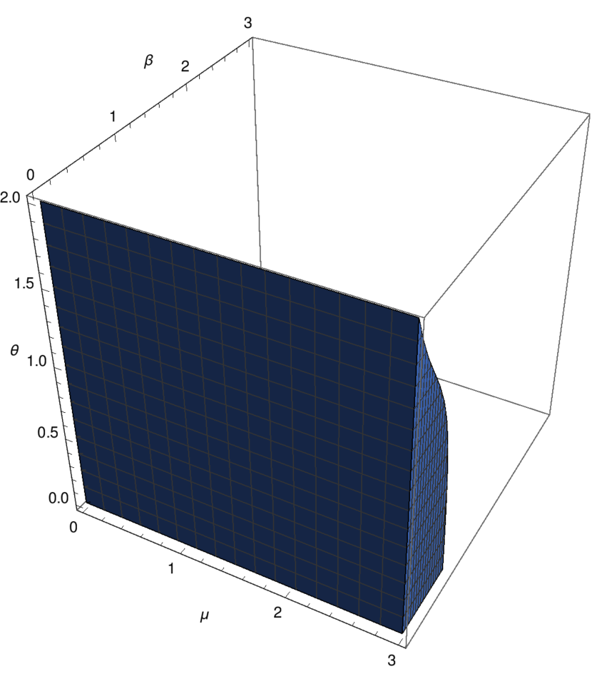
   (a) Case (a)

   

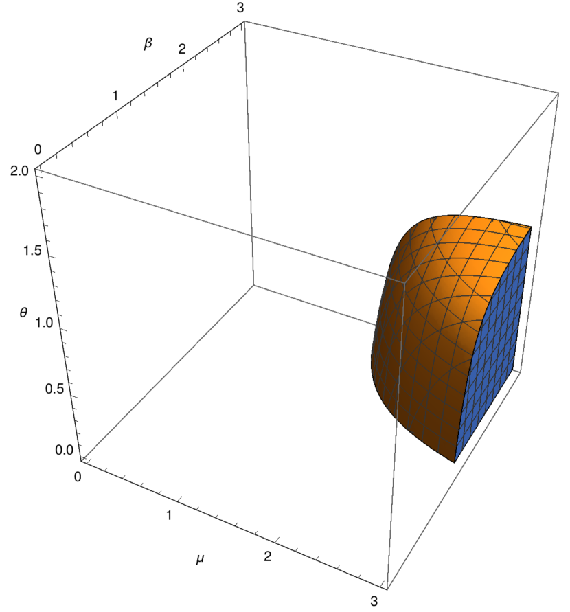
   (b) Case (b)

   

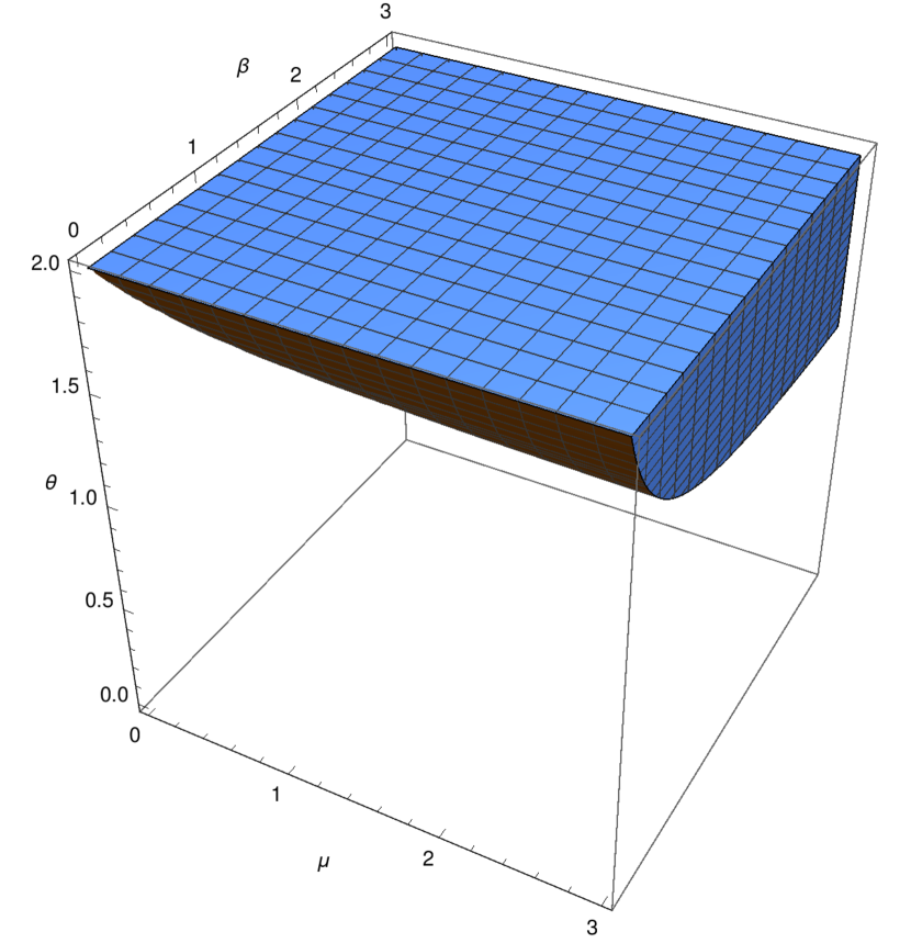
   (c) Case (c)

   

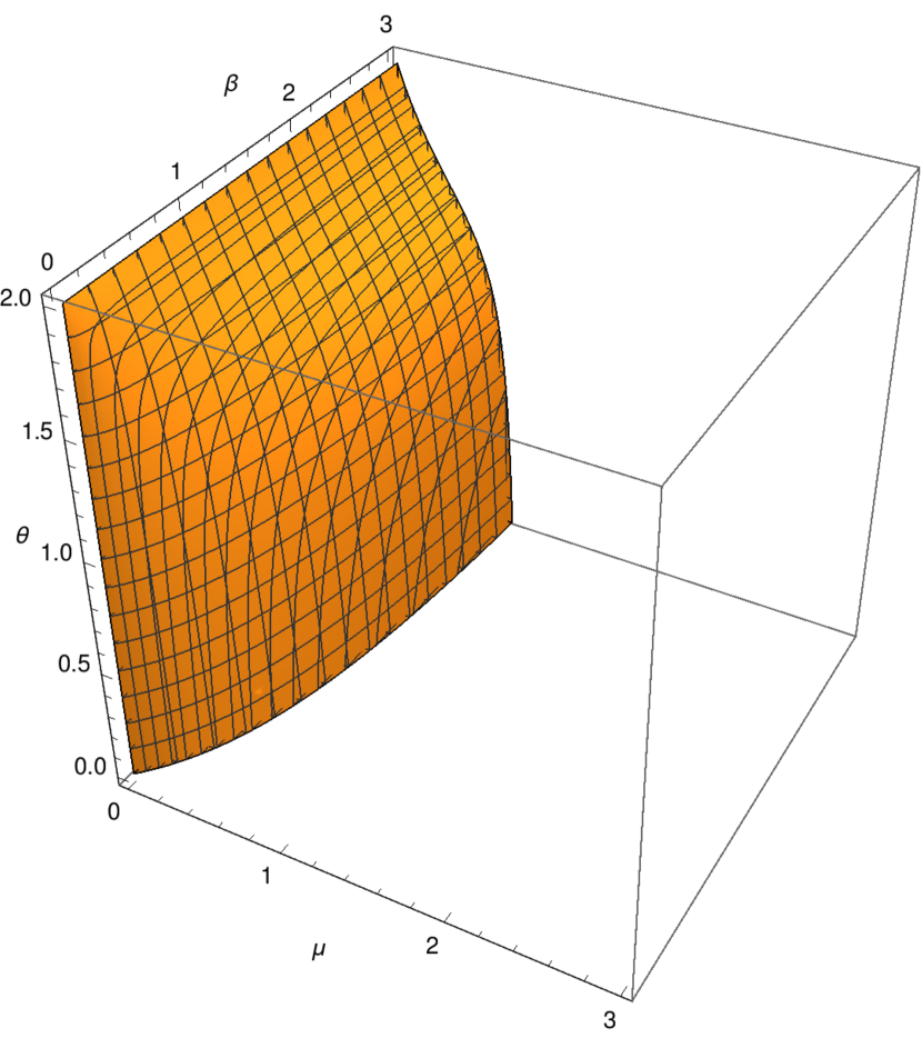
   (d) Case (d)

   

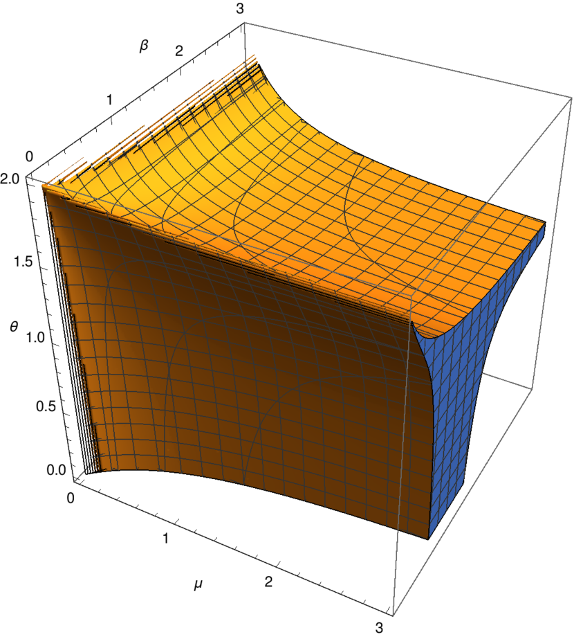
   (e) Case (e)

   Figure 3: Parameter regions for the 5 cases of Theorem 4.1 in the $\mu$-$\beta$-$\theta$ plane.

   

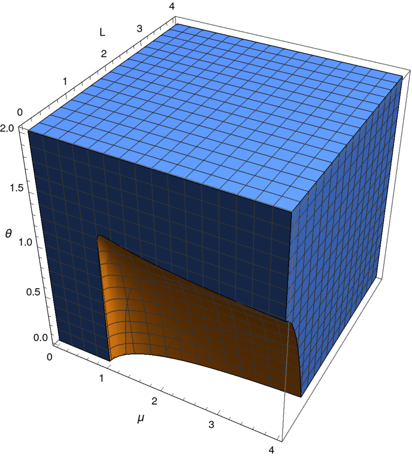
   (a) Case (a)

   

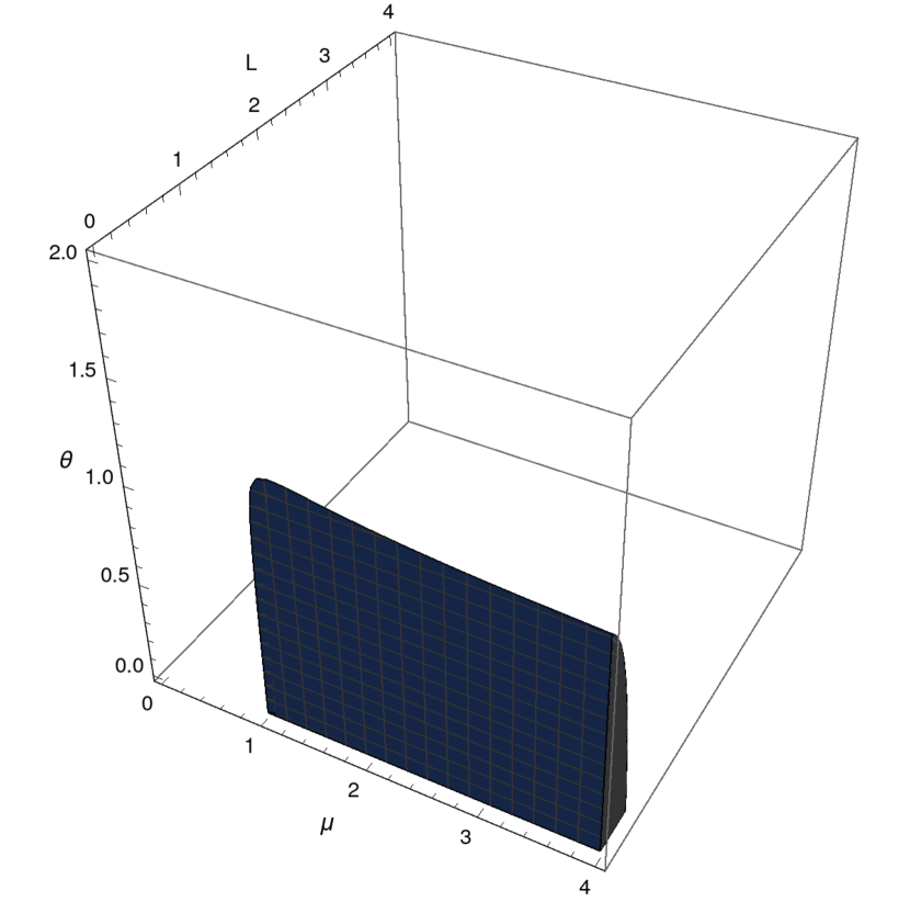
   (b) Case (b)

   

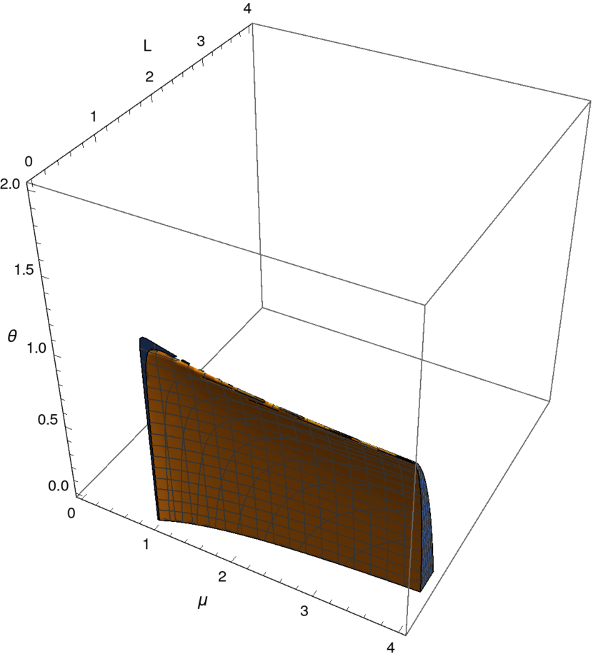
   (c) Case (c)

   Figure 4: Parameter regions for the 3 cases of Theorem 4.4 in the $\mu$-$L$-$\theta$ plane.

   

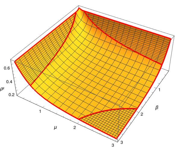
   Figure 5: Contraction factor for Corollary 4.2 (when $\theta=1$) in the $\mu$-$\beta$ plane.

   

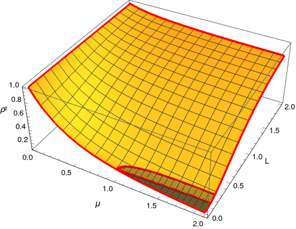
   Figure 6: Contraction factor for Corollary 4.5 (when $\theta=1$) in the $\mu$-$L$ plane.

References

- [1] H. H. Bauschke, Fenchel duality, Fitzpatrick functions and the extension of firmly nonexpansive mappings, Proc. Amer. Math. Soc., 135 (2007), pp. 135–139.
- [2] H. H. Bauschke and P. L. Combettes, Convex Analysis and Monotone Operator Theory in Hilbert Spaces, Springer New York, 2nd ed., 2017.
- [3] H. H. Bauschke and X. Wang, Firmly nonexpansive and Kirszbraun–Valentine extensions: a constructive approach via monotone operator theory, in Nonlinear Analysis and Optimization I: Nonlinear Analysis, American Mathematics Society, 2010, pp. 55–64.
- [4] H. H. Bauschke, X. Wang, and L. Yao, General resolvents for monotone operators: characterization and extension, in Biomedical Mathematics: Promising Directions in Imaging, Therapy Planning, and Inverse Problems, Medical Physics Publishing, 2010, pp. 57–74.
- [5] L. M. Briceño-Arias, Forward-Douglas–Rachford splitting and forward-partial inverse method for solving monotone inclusions, Optimization, 64 (2015), pp. 1239–1261.
- [6] L. M. Briceño-Arias and D. Davis, Forward-backward-half forward algorithm for solving monotone inclusions, SIAM Journal on Optimization, 28 (2018), pp. 2839–2871.
- [7] R. E. Bruck, On the weak convergence of an ergodic iteration for the solution of variational inequalities for monotone operators in Hilbert space, Journal of Mathematical Analysis and Applications, 61 (1977), pp. 159–164.
- [8] G. H.-G. Chen and R. T. Rockafellar, Convergence rates in forward-backward splitting, SIAM Journal on Optimization, 7 (1997), pp. 421–444.
- [9] L. Chen, X. Li, D. Sun, and K.-C. Toh, On the equivalence of inexact proximal ALM and ADMM for a class of convex composite programming, Mathematical Programming, (2019).
- [10] P. Chen, J. Huang, and X. Zhang, A primal-dual fixed point algorithm for minimization of the sum of three convex separable functions, Fixed Point Theory and Applications, 2016 (2016), p. 54.
- [11] J.-P. Crouzeix and E. O. Anaya, Maximality is nothing but continuity, Journal of Convex Analysis, 17 (2010), pp. 521–534.
- [12] J.-P. Crouzeix and E. O. Anaya, Monotone and maximal monotone affine subspaces, Operations Research Letters, 38 (2010), pp. 139–142.
- [13] J.-P. Crouzeix, E. O. Anaya, and W. Sosa, A construction of a maximal monotone extension of a monotone map, ESAIM: Proc., 20 (2007), pp. 93–104.
- [14] E. R. Csetnek, Y. Malitsky, and M. K. Tam, Shadow Douglas–Rachford splitting for monotone inclusions, Applied Mathematics & Optimization, (2019).
- [15] D. Davis and W. Yin, Faster convergence rates of relaxed Reaceman–Rachford and ADMM under regularity assumptions, Mathematics of Operations Research, 42 (2017), pp. 783–805.
- [16] D. Davis and W. Yin, A three-operator splitting scheme and its optimization applications, Set-Valued and Variational Analysis, 25 (2017), pp. 829–858.
- [17] W. Deng and W. Yin, On the global and linear convergence of the generalized alternating direction method of multipliers, Journal of Scientific Computing, 66 (2016), pp. 889–916.
- [18] J. Douglas and H. H. Rachford, On the numerical solution of heat conduction problems in two and three space variables, Transactions of the American Mathematical Society, 82 (1956), pp. 421–439.
- [19] Y. Drori, The exact information-based complexity of smooth convex minimization, Journal of Complexity, 39 (2017), pp. 1–16.
- [20] Y. Drori and M. Teboulle, Performance of first-order methods for smooth convex minimization: a novel approach, Mathematical Programming, 145 (2014), pp. 451–482.
- [21] G. França and J. Bento, An explicit rate bound for over-relaxed ADMM, in Information Theory (ISIT), 2016 IEEE International Symposium on, IEEE, 2016, pp. 2104–2108.
- [22] E. Ghadimi, A. Teixeira, I. Shames, and M. Johansson, On the optimal step-size selection for the alternating direction method of multipliers, IFAC Proceedings Volumes, 45 (2012), pp. 139–144.
- [23] E. Ghadimi, A. Teixeira, I. Shames, and M. Johansson, Optimal parameter selection for the alternating direction method of multipliers (ADMM): Quadratic problems, IEEE Transactions on Automatic Control, 60 (2015), pp. 644–658.
- [24] P. Giselsson, Tight linear convergence rate bounds for Douglas-Rachford splitting and ADMM, in Proceedings of 54th Conference on Decision and Control, Osaka, Japan, Dec 2015.
- [25] P. Giselsson, Tight global linear convergence rate bounds for Douglas–Rachford splitting, Journal of Fixed Point Theory and Applications, 19 (2017), pp. 2241–2270.
- [26] P. Giselsson and S. Boyd, Diagonal scaling in Douglas-Rachford splitting and ADMM, in 53rd IEEE Conference on Decision and Control, Los Angeles, CA, Dec. 2014, pp. 5033–5039.
- [27] P. Giselsson and S. Boyd, Linear convergence and metric selection for Douglas-Rachford splitting and ADMM, IEEE Transactions on Automatic Control, 62 (2017), pp. 532–544.
- [28] A. A. Goldstein, Convex programming in Hilbert space, Bulletin of the American Mathematical Society, 70 (1964), pp. 709–710.
- [29] G. Gu and J. Yang, On the optimal ergodic sublinear convergence rate of the relaxed proximal point algorithm for variational inequalities, arXiv preprint arXiv:1905.06030, (2019).
- [30] G. Gu and J. Yang, On the optimal linear convergence factor of the relaxed proximal point algorithm for monotone inclusion problems, arXiv preprint arXiv:1905.04537, (2019).
- [31] G. Gu and J. Yang, Optimal nonergodic sublinear convergence rate of proximal point algorithm for maximal monotone inclusion problems, arXiv preprint arXiv:1904.05495, (2019).
- [32] D. Han, D. Sun, and L. Zhang, Linear rate convergence of the alternating direction method of multipliers for convex composite programming, Mathematics of Operations Research, 43 (2018), pp. 622–637.
- [33] M. Hong and Z.-Q. Luo, On the linear convergence of the alternating direction method of multipliers, Mathematical Programming, 162 (2017), pp. 165–199.
- [34] R. B. Kellogg, A nonlinear alternating direction method, Mathematics of Computation, 23 (1969), pp. 23–27.
- [35] D. Kim and J. A. Fessler, Optimized first-order methods for smooth convex minimization, Mathematical programming, 159 (2016), pp. 81–107.
- [36] D. Kim and J. A. Fessler, On the convergence analysis of the optimized gradient method, Journal of Optimization Theory and Applications, 172 (2017), pp. 187–205.
- [37] D. Kim and J. A. Fessler, Adaptive restart of the optimized gradient method for convex optimization, Journal of Optimization Theory and Applications, 178 (2018), pp. 240–263.
- [38] D. Kim and J. A. Fessler, Another look at the fast iterative shrinkage/thresholding algorithm (FISTA), SIAM Journal on Optimization, 28 (2018), pp. 223–250.
- [39] D. Kim and J. A. Fessler, Generalizing the optimized gradient method for smooth convex minimization, SIAM Journal on Optimization, 28 (2018), pp. 1920–1950.
- [40] D. Kim and J. A. Fessler, Optimizing the efficiency of first-order methods for decreasing the gradient of smooth convex functions, arXiv preprint arXiv:1803.06600, (2018).
- [41] M. Kirszbraun, Über die zusammenziehende und Lipschitzsche transformationen, Fundamenta Mathematicae, 22 (1934), pp. 77–108.
- [42] G. M. Korpelevich, The extragradient method for finding saddle points and other problems, Ekonomika i Matematicheskie Metody, 12 (1976), pp. 747–756.
- [43] L. Lessard, B. Recht, and A. Packard, Analysis and design of optimization algorithms via integral quadratic constraints, SIAM Journal on Optimization, 26 (2016), pp. 57–95.
- [44] E. S. Levitin and B. T. Polyak, Constrained minimization methods, Zhurnal Vychislitel’noi Matematiki i Matematicheskoi Fiziki, 6 (1966), pp. 787–823.
- [45] F. Lieder, On the convergence rate of the Halpern-iteration, Optimization Online preprint:2017-11-6336, (2017).
- [46] T. Lin, S. Ma, and S. Zhang, An extragradient-based alternating direction method for convex minimization, Foundations of Computational Mathematics, 17 (2017), pp. 35–59.
- [47] P. L. Lions and B. Mercier, Splitting algorithms for the sum of two nonlinear operators, SIAM Journal on Numerical Analysis, 16 (1979), pp. 964–979.
- [48] J. Löfberg, Yalmip : A toolbox for modeling and optimization in matlab, in In Proceedings of the CACSD Conference, Taipei, Taiwan, 2004.
- [49] Y. Malitsky, Golden ratio algorithms for variational inequalities, Mathematical Programming, (2019).
- [50] Y. Malitsky and M. K. Tam, A forward-backward splitting method for monotone inclusions without cocoercivity, arXiv preprint arXiv:1808.04162, (2018).
- [51] B. Mercier, Inéquations variationnelles de la mécanique, Université de Paris-Sud, Département de mathématique, 1980.
- [52] MOSEK ApS, The MOSEK optimization toolbox for MATLAB manual. Version 8.1., 2017, http://docs.mosek.com/8.1/toolbox/index.html.
- [53] W. M. Moursi and L. Vandenberghe, Douglas–Rachford splitting for the sum of a Lipschitz continuous and a strongly monotone operator, Journal of Optimization Theory and Applications, 183 (2019), pp. 179–198.
- [54] R. Nishihara, L. Lessard, B. Recht, A. Packard, and M. Jordan, A general analysis of the convergence of ADMM, in Proceedings of the 32nd International Conference on Machine Learning, vol. 37 of Proceedings of Machine Learning Research, 2015, pp. 343–352.
- [55] G. B. Passty, Ergodic convergence to a zero of the sum of monotone operators in Hilbert space, Journal of Mathematical Analysis and Applications, 72 (1979), pp. 383–390.
- [56] D. W. Peaceman and H. H. Rachford, The numerical solution of parabolic and elliptic differential equations, Journal of the Society for Industrial and Applied Mathematics, 3 (1955), pp. 28–41.
- [57] F. Pedregosa, On the convergence rate of the three operator splitting scheme, arXiv preprint arXiv:1610.07830, (2016).
- [58] F. Pedregosa, K. Fatras, and M. Casotto, Proximal splitting meets variance reduction, 2019.
- [59] F. Pedregosa and G. Gidel, Adaptive three operator splitting, in Proceedings of the 35th International Conference on Machine Learning, J. Dy and A. Krause, eds., vol. 80 of Proceedings of Machine Learning Research, PMLR, 10–15 Jul 2018, pp. 4085–4094.
- [60] H. Raguet, A note on the forward-Douglas–Rachford splitting for monotone inclusion and convex optimization, Optimization Letters, (2018).
- [61] H. Raguet, J. Fadili, and G. Peyré, A generalized forward-backward splitting, SIAM Journal on Imaging Sciences, 6 (2013), pp. 1199–1226.
- [62] S. Reich, Extension problems for accretive sets in Banach spaces, Journal of Functional Analysis, 26 (1977), pp. 378–395.
- [63] S. Reich and S. Simons, Fenchel duality, Fitzpatrick functions and the Kirszbraun–Valentine extension theorem, Proceedings of the American Mathematical Society, 133 (2005), pp. 2657–2660.
- [64] J. Rieger and M. K. Tam, Backward-forward-reflected-backward splitting for three operator monotone inclusions, arXiv:2001.07327, (2020).
- [65] R. Rockafellar, Conjugate Duality and Optimization, Society for Industrial and Applied Mathematics, 1974.
- [66] E. K. Ryu and S. Boyd, Primer on monotone operator methods, Appl. Comput. Math., 15 (2016), pp. 3–43.
- [67] E. K. Ryu, R. Hannah, and W. Yin, Scaled relative graph: Nonexpansive operators via 2D Euclidean geometry, arXiv preprint arXiv:1902.09788, (2019).
- [68] E. K. Ryu and B. C. Vũ, Finding the forward-Douglas–Rachford-forward method, Journal of Optimization Theory and Applications, (2019).
- [69] J. H. Seidman, M. Fazlyab, V. M. Preciado, and G. J. Pappas, A control-theoretic approach to analysis and parameter selection of Douglas–Rachford splitting, IEEE Control Systems Letters, 4 (2020), pp. 199–204.
- [70] A. Taylor, B. Van Scoy, and L. Lessard, Lyapunov functions for first-order methods: Tight automated convergence guarantees, in Proceedings of the 35th International Conference on Machine Learning, vol. 80, PMLR, 2018, pp. 4897–4906.
- [71] A. B. Taylor, J. M. Hendrickx, and F. Glineur, Exact worst-case performance of first-order methods for composite convex optimization, SIAM Journal on Optimization, 27 (2017), pp. 1283–1313.
- [72] A. B. Taylor, J. M. Hendrickx, and F. Glineur, Performance estimation toolbox (PESTO): automated worst-case analysis of first-order optimization methods, in 2017 IEEE 56th Annual Conference on Decision and Control (CDC), IEEE, 2017, pp. 1278–1283.
- [73] A. B. Taylor, J. M. Hendrickx, and F. Glineur, Smooth strongly convex interpolation and exact worst-case performance of first-order methods, Mathematical Programming, 161 (2017), pp. 307–345.
- [74] A. B. Taylor, J. M. Hendrickx, and F. Glineur, Exact worst-case convergence rates of the proximal gradient method for composite convex minimization, Journal of Optimization Theory and Applications, 178 (2018), pp. 455–476.
- [75] A. Teixeira, E. Ghadimi, I. Shames, H. Sandberg, and M. Johansson, Optimal scaling of the ADMM algorithm for distributed quadratic programming, in 52nd IEEE Conference on Decision and Control, 2013, pp. 6868–6873.
- [76] A. Teixeira, E. Ghadimi, I. Shames, H. Sandberg, and M. Johansson, The ADMM algorithm for distributed quadratic problems: Parameter selection and constraint preconditioning, IEEE Transactions on Signal Processing, 64 (2016), pp. 290–305.
- [77] P. Tseng, Applications of a splitting algorithm to decomposition in convex programming and variational inequalities, SIAM Journal on Control and Optimization, 29 (1991), pp. 119–138.
- [78] P. Tseng, A modified forward-backward splitting method for maximal monotone mappings, SIAM Journal on Control and Optimization, 38 (2000), pp. 431–446.
- [79] F. A. Valentine, On the extension of a vector function so as to preserve a Lipschitz condition, Bull. Amer. Math. Soc., 49 (1943), pp. 100–108.
- [80] F. A. Valentine, A Lipschitz condition preserving extension for a vector function, American Journal of Mathematics, 67 (1945), pp. 83–93.
- [81] B. Van Scoy, R. A. Freeman, and K. M. Lynch, The fastest known globally convergent first-order method for minimizing strongly convex functions, IEEE Control Systems Letters, 2 (2018), pp. 49–54.
- [82] H. Wang, M. Fazlyab, S. Chen, and V. M. Preciado, Robust convergence analysis of three-operator splitting, arXiv preprint arXiv:1910.04229, (2019).
- [83] X. Wang and L. Yao, Maximally monotone linear subspace extensions of monotone subspaces: explicit constructions and characterizations, Mathematical Programming, 139 (2013), pp. 327–352.
- [84] M. Yan, A new primal-dual algorithm for minimizing the sum of three functions with a linear operator, Journal of Scientific Computing, 76 (2018), pp. 1698–1717.