Upper bound on the duration of quantum jumps

Abstract

We present a method to estimate the time scale of quantum jumps from the time correlation of photon pairs generated from a cascade decay in an atomic system, and realize it experimentally in a cold cloud of ⁸⁷Rb. Taking into account the photodetector response, we find an upper bound for the duration of a quantum jump of $21\pm 11$ ps.

Introduction – The concept of quantum jumps is traced back to Bohr and the old quantum theory Bohr (1913). This theory found its bases on Planck’s hypothesis of energy quanta and lead to successful explanations of the photoelectric effect, discrete atomic spectra, and distribution of a blackbody in thermal equilibrium. While it described the discrete states of systems accurately, the theory raised questions regarding the transition periods—or quantum jumps—between states. The periods occurred at random times and, by considering intermediate states forbidden, they had to be instantaneous. The general inadequacy of the old quantum theory appeared to be fixed by wave mechanics Schrödinger (1952); yet, for quantum systems under observation, it has not been possible to depart completely from the quantum jump concept Bell (1987).

The idea for early observations of quantum jumps was seeded on Dehmelt’s electron shelving proposal Dehmelt (1975), where the fluorescence of a driven two-state system is abruptly interrupted as the system transitions to a third, metastable, state. This scheme has been implemented for single trapped ions Nagourney et al. (1986); Sauter et al. (1986); Bergquist et al. (1986) and neutral atoms Finn et al. (1986). Recent quantum jump experiments involve nuclear spins Neumann et al. (2010), cavity–Gleyzes et al. (2007) and circuit Vijay et al. (2011); Minev et al. (2018) quantum electrodynamics architectures. In all these demonstrations, the evolution of the monitored variable has the form of a telegraphic signal Cook and Kimble (1985) presenting on and off times whose duration can be described quantitatively through a study of the waiting time-distribution Cohen-Tannoudji and Dalibard (1986) and applying photodetection theory Glauber (1963); Javanainen (1986). Since the probability for a system to be found in a particular state is conditioned to a given measurement record, the inferred transition times reflect the way the system is monitored Carmichael (1991); Wiseman and Milburn (1993). Apart from studies based on the photoelectric effect Ossiander et al. (2016, 2018), the time structure of the rise and descend transitions has been rarely explored at the limits of contemporary experimental capabilities Minev et al. (2018).

In this work we focus on quantum jumps associated to spontaneous transitions involving discrete states. We consider an alternative configuration for the observation of quantum jumps in atomic systems: a monitored cascade three-level system Javanainen (1986); Hendriks and Nienhuis (1988). Contrary to the shelving configuration, where the transition to the metastable state is inferred from the absence of a fluorescent signal, i.e., a null measurement Pegg (1991); Porrati and Putterman (1987), state information in a cascade system is acquired through the detection of correlated photon pairs with a well-defined time ordering. This, coupled with the fact that phase matching conditions allow for photon coincidences to be accurately measured, makes the cascade configuration ideal to experimentally investigate the discontinuous changes in atomic states.

We observe the quantum jumps in the second order time correlation function of the fluorescence generated by a cascade-based four-wave mixing (FWM) in a cold ensemble of ⁸⁷Rb, and model the experiment as a cascade three-level system via the adiabatic elimination of one of the intermediate states. To improve the timing precision for observing any possible jump dynamics, we take into account the measured impulse response of the single photon detectors for estimating an upper bound on the duration of the quantum jump from the measured time correlation.

Theory – Consider a four-level system in the diamond configuration as depicted in Fig. 1. For ⁸⁷Rb, the atomic ground state $5S_{1/2}$, level $|0\rangle$, is coupled to an excited state $5D_{3/2}$, $|2\rangle$, through a two-step excitation and decay process involving the intermediate levels $5P_{3/2}$, $|1\rangle$, and $5P_{1/2}$, $|3\rangle$. The excitation path $|0\rangle\leftrightarrow|1\rangle\leftrightarrow|2\rangle$ is coherently driven by a pair of non-resonant lasers, while coupling to the electromagnetic environment induces the de-excitation path $|2\rangle\rightarrow|3\rangle\rightarrow|0\rangle$ through spontaneous emission of idler and signal photons. Due to the collective nature of the process, a phase-matching condition of the cascade emission allows to efficiently collect the light used to monitor the atomic state.

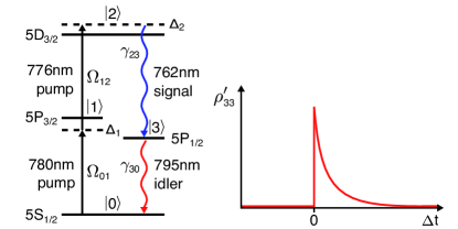
Figure 1: (Left) Atomic level configuration in a four-wave mixing experiment. (Right) Time evolution of the population of level $|3\rangle$, conditioned on the detection of a signal photon according to Eq. (7).

The joint probability distribution to detect a heralding photon in mode $s$ at time $t$ and a correlated photon in mode $i$ at time $t+\Delta t$ is related to the correlation function

$$C(t,t+\Delta t)=\langle\hat{a}^{\dagger}_{s}(t)\hat{a}^{\dagger}_{i}(t+\Delta t)\hat{a}_{i}(t+\Delta t)\hat{a}_{s}(t)\rangle\,\,,$$ (1)

with the annihilation and creation operators $\hat{a}_{s,i}$ and $\hat{a}^{\dagger}_{s,i}$ of the $s$ and $i$ modes. For an electromagnetic environment in the vacuum state, the correlation function $C$ is proportional to the atomic polarization correlation

$${P}(t,t+\Delta t)=\langle\hat{\sigma}^{\dagger}_{23}(t)\hat{\sigma}^{\dagger}_{30}(t+\Delta t)\hat{\sigma}_{30}(t+\Delta t)\hat{\sigma}_{23}(t)\rangle\,,$$ (2)

with the lowering operator $\hat{\sigma}_{ij}\equiv|j\rangle\langle i|$ describing transitions from the atomic level $|i\rangle$ to level $|j\rangle$ in the Heisenberg picture. Using the quantum regression theorem Lax (1968) it is possible to show that

$${P}(t,t+\Delta t)=\rho_{22}(t)\rho^{\prime}_{33}(t+\Delta t)\,,$$ (3)

so that atomic density matrix element $\rho_{22}(t)$ represents the population of state $|2\rangle$ at time $t$, while $\rho^{\prime}_{33}(t+\Delta t)$ that of state $|3\rangle$ at time $t+\Delta t$ under the initial condition $\rho^{\prime}_{33}(t)=|3\rangle\langle 3|$. This result reflects the well-defined time order that allows the study of quantum jumps in the four-wave mixing process.

It is possible to obtain an analytical expression for ${P}(t,t+\Delta t)$; its derivation, however, is greatly simplified if the intermediate level $|1\rangle$ is adiabatically eliminated. This elimination is valid for far-detuned lasers, which induce rapid oscillations on the probability amplitude to find the system in the intermediate level and allow us to consider its zero average value. Under this approximation, the system maps to an effective three-level cascade system with an evolution ruled by the master equation:

$$\dot{\rho}=(i\hbar)^{-1}\left[\mathcal{H}_{\text{eff}},\rho\right]+\sum_{n,m}\gamma_{nm}\left[2\hat{\sigma}_{nm}\rho\hat{\sigma}_{nm}^{\dagger}-\hat{\sigma}_{nn}\rho-\rho\hat{\sigma}_{nn}\right]\,,$$ (4)

with the effective Hamiltonian

$$\mathcal{H}_{\text{eff}}=\hbar\Delta_{\text{eff}}|2\rangle\langle 2|+\sum_{i=2,3}E_{i}|i\rangle\langle i|+\frac{\hbar\Omega_{\text{eff}}}{2}\left(|2\rangle\langle 0|+|0\rangle\langle 2|\right)\,,$$ (5)

and effective detuning and Rabi frequency

$$\Delta_{\text{eff}}=\Delta_{2}+\frac{\Omega_{01}^{2}}{4\Delta_{1}}-\frac{\Omega_{12}^{2}}{4\Delta_{1}}\,\quad\text{and}\quad\Omega_{\text{eff}}=-\frac{\Omega_{01}\Omega_{12}}{2\Delta_{1}}\,.$$ (6)

In these expressions, $\Omega_{ij}$ denote the bare Rabi frequencies for the induced $|i\rangle\leftrightarrow|j\rangle$ transitions, $\gamma_{ij}$ the spontaneous decay rates, and $\Delta_{i}$ the detuning between the driving lasers and the atomic resonances $(E_{i}-E_{j})/\hbar$. The master equation evolution is equivalent to a solvable set of algebraic equations obtained using the Laplace transform, allowing for the calculation of analytical expressions that describe the evolution of the density matrix. With the initial condition $\rho^{\prime}_{33}(t_{0})=1$ where $t_{0}$ is the time at which the signal photon is detected, and for the experimental parameters shown below one finds

$$\rho^{\prime}_{33}(t_{0}+\Delta t) =0\quad {\mathrm{for}} \Delta t<0\,,$$ (7)

$$\rho^{\prime}_{33}(t_{0}+\Delta t) \approx e^{-\left(\gamma_{30}+\tfrac{\gamma_{23}}{2}\right)\Delta t}\quad {\mathrm{for}} \Delta t>0\,,$$

while $\rho_{22}(t)$ is a continuous function of $t$. Thus, the correlation function $P(t,t+\Delta t)$ exhibits a discontinuity at $\Delta t=0$ that reflects the breaking of time symmetry induced by the quantum jump associated to the transition $|2\rangle\rightarrow|3\rangle$. For $\Delta t>0$ the atom can perform a second jump to the ground state with statistics given by $\rho^{\prime}_{33}$ in Eq. (7).

Signal and idler photons impinge on photon detectors that, while able to distinguish between either mode, are unable to determine with certainty the hyperfine level they were emitted from. This indeterminacy causes that the atomic state conditioned to the detection of a signal photon is given by a superposition of the hyperfine states of level $|1\rangle$, i.e., $5P_{1/2}$ $F=1$ and $F=2$ states. This yields oscillations of $\rho^{\prime}_{33}(t_{0}+\Delta t)$ for $\Delta t>0$ with a frequency determined by the beating frequencies of these hyperfine levels Gulati et al. (2015). These quantum beats can be well reproduced with our model by numerically solving the Bloch equations for a density matrix that involves all hyperfine sublevels of the $|i\rangle$, i=0,1,2,3 states. The frequency and amplitude of the quantum beats are highly sensitive to the polarization, intensity and detuning of the pump lasers. Details of the calculations will be provided in a forthcoming publication. Important to notice here is that the observation of quantum beats provides a striking evidence of quantum coherence.

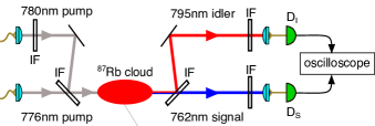
Figure 2: Schematic of the four-wave mixing experiment. IF: interference filters to combine pump beams and to separate the photons pairs; D_S, D_I: silicon avalanche photodiodes (APD).

Experiment – Figure 2 shows schematically the experimental setup for generating time-ordered photon pairs by four-wave mixing in a cold ensemble of ⁸⁷Rb atoms. Pump beams at 780 nm and 776 nm excite atoms from the $5S_{1/2},F=2$ ground level to the $5D_{3/2},F=3$ level via a two-photon transition. The signal (762 nm) and idler (795 nm) photons emerge from a cascade decay back to the ground level through the $5P_{1/2}$ level, and are coupled to single mode fibers. Phase matching between pump and target modes is ensured with all four modes propagating in the same direction. The two pump modes are almost collimated and have a Gaussian beam waist of about 400 $\mu$m in the atomic cloud. The linearly polarized pump mode at 780 nm is red-detuned by 40 MHz from the $5S_{1/2},F=2$ to $5P_{3/2},F=3$ transition and has an optical power of 0.5 mW. The orthogonally polarized pump mode at 776 nm shares the same optical mode, has an optical power of 6.5 mW, and is tuned such that the two-photon excitation is blue-detuned by 4 MHz from the difference between the ground state and the $5D_{3/2},F=3$ level. We record the detection event time differences of the photon pairs with a digital oscilloscope (sampling rate $4\times 10^{10}\,\text{s}^{-1}$) with an effective time resolution below 10 ps; the single photon avalanche detectors themselves have a nominal timing jitter around 50 ps FWHM.

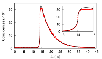
Figure 3: Histogram $G_{\mathrm{FWM}}(\Delta t)$ of detection time differences for photons pairs generated by four-wave mixing in the cold cloud of ⁸⁷Rb. The continuous line shows the result of the best fit of Eq. (10). Inset: detail of the sharp rise corresponding to a quantum jump.

Figure 3 shows the histogram $G_{\mathrm{FWM}}(\Delta t)$ of signal and idler photodetection time differences $\Delta t$ into 10 ps wide bins. The expected exponential decay starts at $\Delta t_{0}\approx 14$ ns due to technical delays through fibers and cables. The decay time constant is shorter than the natural decay time $1/\gamma_{30}\approx 27$ ns and determined by the number of atoms involved and the detuning of the pump fields Srivathsan et al. (2013); Cerè et al. (2018). The oscillations on top of the exponential decay are due to quantum beats between the transition of interest and alternative decay paths involving nearby hyperfine levels Gulati et al. (2015). The onset of the fluorescence in the idler mode, reflecting the quantum jump, shows a rise time much faster than the time scales of the transitions involved, commensurate with the time jitter of the avalanche photodetectors (see inset of Fig. 3).

To improve the time resolution for observing the quantum jump, we characterize the detector response function.

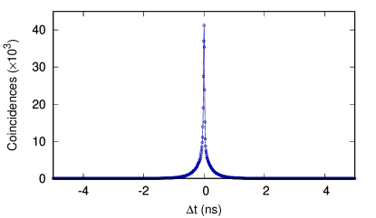
Figure 4: Histogram $G_{\mathrm{D}}(\Delta t)$ of the difference in detection time for photons pairs generated by spontaneous parametric down-conversion in a nonlinear optical crystal. The bandwidth of the photon pair exceeds 20 nm, corresponding to a coherence time of about 0.1 ps. Thus, we can take the measured time correlation as a reasonable approximation for the impulse response of the two-detector system.

For this, we direct photon pairs with a large optical bandwidth generated by spontaneous parametric down-conversion (SPDC) in a nonlinear optical crystal onto the two avalanche photodetectors. The SPDC source is based on $\beta$-Barium Borate, cut for non-degenerate type-I phase matching. Pumped with light at 405 nm, it generates time-correlated photon pairs at 770 nm and 854 nm Villar et al. (2018). The measured bandwidths (23 nm and 32 nm, respectively) correspond to a coherence time of the down-converted photon pairs below 0.1 ps, a negligible contribution to  $G_{\mathrm{D}}(\Delta t)$ in comparison to the detector response time scale. The resulting calibration coincidence histogram $G_{\mathrm{D}}(\Delta t)$ into 10 ps wide bins is shown in Fig. 4. Despite the wavelength difference, $G_{\mathrm{D}}(\Delta t)$ does not show any appreciable asymmetry. From this, we infer that the timing response of the detectors does not vary significantly over this wavelength range, and we thus expect that the measured behavior is a good approximation of the detector timing characteristics for photons at 762 nm and 795 nm.

Result – While the structure of $G_{\mathrm{FWM}}(\Delta t)$ away from $\Delta t=0$ is well understood, we have no model for a possible dynamic of the jump itself. In order to associate a time scale to the transient behavior, we join the two parts of Eq. (7) with a smooth heuristic transition

$$\sigma(x)\>=\>\frac{1}{1+\exp\left(-x\right)}\,.$$ (8)

The choice of $\sigma(x)$ is not inspired by a specific dynamical model, its only purpose is to establish a time scale for the transient. This particular form is attractive since it admits the step function as a limiting scenario. The atomic state, with the exponential decay with time constant $\tau$ described by Eq. (7), is then enclosed in the monitor function

$$y(\Delta t;\alpha,\tau)\>=\>\sigma\!\left(\frac{\Delta t}{\alpha}\right)\,\exp\left(-\frac{\Delta t}{\tau}\right)\,,$$ (9)

where the jump timescale is characterized by $\alpha$.

By convolving the monitoring function $y(\Delta t)$ in Eq. (9) with the normalized measured detector response $g_{\mathrm{D}}(\Delta t)=G_{\mathrm{D}}(\Delta t)/\sum G_{\mathrm{D}}(\Delta t)$, we construct a model $Y$ for the observed $G_{\mathrm{FWM}}(\Delta t)$ in Fig. 3,

$$Y(\Delta t)\>=\>A\>y(\Delta t-\Delta t_{0};\alpha,\tau)*g_{\mathrm{D}}(\Delta t)+Y_{0}\,$$ (10)

with amplitude $A$, decay time $\tau$, accidental coincidence background $Y_{0}$, time delay $\Delta t_{0}$, and characteristic time $\alpha$ for the jump. We then use $A$, $Y_{0}$, $\Delta t_{0}$, and $\alpha$ as free parameters to fit $Y(\Delta t)$ to our measured time difference distribution. This fit, shown as continuous line in Fig. 3, results in $\alpha=4.7\pm 2.5$ ps corresponding to a 10%–90% rise time associated with the jump of $21\pm 11$ ps.

Conclusion – We establish a bound for the duration of a quantum jump based on the observed onset of time correlations between photons emitted from an atomic cascade decay in a cold cloud of ⁸⁷Rb. We find a value that is about three orders of magnitude shorter than the natural lifetime of the involved atomic states, and four orders of magnitude longer than an optical cycle.

In comparison with other techniques Nagourney et al. (1986); Sauter et al. (1986); Bergquist et al. (1986); Finn et al. (1986); Neumann et al. (2010); Gleyzes et al. (2007); Vijay et al. (2011); Minev et al. (2018), there seems to be no fundamental limit to the time resolution of this method down to the time scale of the photoelectric effect. We believe our measurement is still limited by the uncertainty in the time response of the avalanche photodetectors, and potentially far from the timescale of quantum jumps – should there be one. Adoption of faster and better characterized detectors, for example from a recent generation of superconducting nanowires Shcheslavskiy et al. (2016), has the potential to significantly improve the time resolution of such an experiment, and possibly establish or abandon a resolvable time scale for quantum jumps.

References

- Bohr (1913) N. Bohr, The London, Edinburgh, and Dublin Philosophical Magazine and Journal of Science 26, 1 (1913).
- Schrödinger (1952) E. Schrödinger, Br J Philos Sci III, 233 (1952).
- Bell (1987) J. Bell, “Are there quantum jumps?” in Schrödinger: Centenary Celebration of a Polymath, edited by C. W. Kilmister (Cambridge University Press, 1987) pp. 41–52.
- Dehmelt (1975) H. G. Dehmelt, Bull. Am. Phys. Soc. 20, 60 (1975).
- Nagourney et al. (1986) W. Nagourney, J. Sandberg, and H. Dehmelt, Phys. Rev. Lett. 56, 2797 (1986).
- Sauter et al. (1986) T. Sauter, W. Neuhauser, R. Blatt, and P. E. Toschek, Phys. Rev. Lett. 57, 1696 (1986).
- Bergquist et al. (1986) J. C. Bergquist, R. G. Hulet, W. M. Itano, and D. J. Wineland, Phys. Rev. Lett. 57, 1699 (1986).
- Finn et al. (1986) M. A. Finn, G. W. Greenlees, and D. A. Lewis, Opt. Commun. 60, 149 (1986).
- Neumann et al. (2010) P. Neumann, J. Beck, M. Steiner, F. Rempp, H. Fedder, P. R. Hemmer, J. Wrachtrup, and F. Jelezko, Science 329, 542 (2010).
- Gleyzes et al. (2007) S. Gleyzes, S. Kuhr, C. Guerlin, J. Bernu, S. Deléglise, U. B. Hoff, M. Brune, J.-M. Raimond, and S. Haroche, Nature 446, 297 (2007).
- Vijay et al. (2011) R. Vijay, D. H. Slichter, and I. Siddiqi, Phys. Rev. Lett. 106, 110502 (2011).
- Minev et al. (2018) Z. K. Minev, S. O. Mundhada, S. Shankar, P. Reinhold, R. Gutierrez-Jauregui, R. J. Schoelkopf, M. Mirrahimi, H. J. Carmichael, and M. H. Devoret, arXiv (2018), 1803.00545 .
- Cook and Kimble (1985) R. J. Cook and H. J. Kimble, Phys. Rev. Lett. 54, 1023 (1985).
- Cohen-Tannoudji and Dalibard (1986) C. Cohen-Tannoudji and J. Dalibard, EPL 1, 441 (1986).
- Glauber (1963) R. J. Glauber, Phys. Rev. 130, 2529 (1963).
- Javanainen (1986) J. Javanainen, Phys. Scr. 1986, 67 (1986).
- Carmichael (1991) H. Carmichael, An open systems approach to quantum optics, Lecture Notes in Physics Monographs (Springer, Berlin, 1991).
- Wiseman and Milburn (1993) H. M. Wiseman and G. J. Milburn, Phys. Rev. A 47, 1652 (1993).
- Ossiander et al. (2016) M. Ossiander, F. Siegrist, V. Shirvanyan, R. Pazourek, A. Sommer, T. Latka, A. Guggenmos, S. Nagele, J. Feist, J. Burgdörfer, R. Kienberger, and M. Schultze, Nature Physics 13, 280 (2016).
- Ossiander et al. (2018) M. Ossiander, J. Riemensberger, S. Neppl, M. Mittermair, M. Schäffer, A. Duensing, M. S. Wagner, R. Heider, M. Wurzer, M. Gerl, M. Schnitzenbaumer, J. V. Barth, F. Libisch, C. Lemell, J. Burgdörfer, P. Feulner, and R. Kienberger, Nature 561, 374 (2018).
- Hendriks and Nienhuis (1988) B. H. W. Hendriks and G. Nienhuis, Journal of Modern Optics 35, 1331 (1988).
- Pegg (1991) D. T. Pegg, Physics Letters A 153, 263 (1991).
- Porrati and Putterman (1987) M. Porrati and S. Putterman, Phys. Rev. A 36, 929 (1987).
- Lax (1968) M. Lax, Phys. Rev. 172, 350 (1968).
- Gulati et al. (2015) G. K. Gulati, B. Srivathsan, B. Chng, A. Cerè, and C. Kurtsiefer, New J. Phys. 17, 093034 (2015).
- Srivathsan et al. (2013) B. Srivathsan, G. K. Gulati, B. Chng, G. Maslennikov, D. Matsukevich, and C. Kurtsiefer, Phys. Rev. Lett. 111, 123602 (2013).
- Cerè et al. (2018) A. Cerè, B. Srivathsan, G. K. Gulati, B. Chng, and C. Kurtsiefer, Phys. Rev. A 98, 023835 (2018).
- Villar et al. (2018) A. Villar, A. Lohrmann, and A. Ling, Opt. Express 26, 12396 (2018).
- Shcheslavskiy et al. (2016) V. Shcheslavskiy, P. Morozov, A. Divochiy, Y. Vakhtomin, K. Smirnov, and W. Becker, Rev. Sci. Instrum. 87, 053117 (2016).