Nebular Spectroscopy of Kepler’s Brightest Supernova

Abstract

We present late-time ($\sim$240–260 days after peak brightness) optical photometry and nebular (+236 and +264 days) spectroscopy of SN 2018oh, the brightest Type Ia supernova (SN Ia) observed by the Kepler telescope. The Kepler/K2 30-minute cadence observations started days before explosion and continued past peak brightness. For several days after explosion, SN 2018oh had blue “excess” flux in addition to a normal SN rise. The flux excess can be explained by the interaction between the SN and a Roche-lobe filling non-degenerate companion star. Such a scenario should also strip material from the companion star, that would emit once the SN ejecta become optically thin, imprinting relatively narrow emission features in its nebular spectrum. We search our nebular spectra for signs of this interaction, including close examination of wavelengths of hydrogen and helium transitions, finding no significant narrow emission. We place upper limits on the luminosity of these features of $2.6,\ 2.9\ \mathrm{and}\ 2.1\times 10^{37}\ \mathrm{erg\ s^{-1}}$ for H$\alpha$, He I $\lambda$5875, and He I $\lambda$6678, respectively. Assuming a simple models for the amount of swept-up material, we estimate upper mass limits for hydrogen of $5.4\times 10^{-4}\ \mathrm{M_{\odot}}$ and helium of $4.7\times 10^{-4}\ \mathrm{M_{\odot}}$. Such stringent limits are unexpected for the companion-interaction scenario consistent with the early data. No known model can explain the excess flux, its blue color, and the lack of late-time narrow emission features.

1 Introduction

The exact nature of the progenitor system for Type Ia supernovae (SNe Ia) (the “progenitor problem”) remains one of the most persistent open questions in stellar evolution. Despite decades of research related to this question, and while SNe Ia still constitute an extremely powerful probe for measuring the expansion history of the Universe and determine crucial cosmological parameters (e.g., Riess et al., 2016; Jones et al., 2018; Scolnic et al., 2018; DES Collaboration et al., 2018), the stellar systems that lead to the thermonuclear explosion of the carbon/oxygen white dwarf (WD; Hoyle & Fowler, 1960; Colgate & McKee, 1969; Woosley et al., 1986) and the associated explosion mechanisms are unclear.

In general, two main channels of progenitor systems have been proposed: the single-degenerate (SD) scenario, where the WD explodes due to a thermonuclear runaway near the Chandrasekhar mass ($\mathrm{M_{Ch}}$) by accreting material from a non-degenerate companion (e.g., Whelan & Iben, 1973), and the double-degenerate (DD) scenario, where the SN results from the merger of two WDs (e.g.; Iben & Tutukov, 1984). Confusing the matter, radiative transfer calculations of explosion models from both scenarios are able to broadly reproduce the basic photometric and spectroscopic properties of SNe Ia (e.g. Kasen et al., 2009; Woosley & Kasen, 2011; Hillebrandt et al., 2013; Sim et al., 2013). We have not yet directly observed the progenitor system of a SN Ia, and thus we must rely on indirect measures.

Kasen (2010) showed that if the progenitor system contains a non-degenerate, Roche-Lobe filling companion, the SN ejecta will collide with the companion star, and the shock interaction at its surface will produce strong X-ray/UV emission at the first days after the explosion detectable for some viewing angles. This will result in a luminosity excess beyond the flux expected from the main source of the SN luminosity, ⁵⁶Ni radioactive decay. Observationally, this manifests as a two-component rising light curve, with varying component strengths and durations that depend on the size of the companion, the separation of the binary, and the viewing angle.

Additionally for such a scenario, material from the companion’s surface will be swept up by the ejecta. Once the ejecta become optically thin, the companion-star material will emit producing strong, relatively narrow emission features superimposed on an otherwise typical nebular SN Ia spectrum. Starting with Marietta et al. (2000), who were the first to indicate that this emission is anticipated, several theoretical models and simulations have been developed (e.g., Pan et al., 2012; Liu et al., 2013; Lundqvist et al., 2013; Botyánszki et al., 2018), predicting emission lines of H$\alpha$, He I $\lambda\lambda 5875$,6678, [O I] $\lambda\lambda 6300$,6364 and/or [Ca II] $\lambda\lambda 7291$,7324, depending on the nature of the companion (whether it is a main-sequence, red-giant or helium star) and the properties of the binary system, with different treatments of the simulations predicting varying strengths and shapes of the emission lines.

These two observational diagnostics have been the subject of numerous studies of early- and late-time SN Ia observations. Statistical sample studies (Hayden et al., 2010; Ganeshalingam et al., 2011; González-Gaitán et al., 2012; Firth et al., 2015; Olling et al., 2015) of the early rise times have found slight deviations from the expected $L\propto t^{2}$ law (Arnett, 1982; Riess et al., 1999), attributed to moderate mixing of radioactive ⁵⁶Ni into the outer-most layers of the explosion.

Focusing on individual events, SNe 2009ig (Foley et al., 2012a) and 2011fe (Nugent et al., 2011; Bloom et al., 2012) exhibit the expected smomth single-power-law rise of the ligth curve (close to $L\propto t^{2}$) with red early-time colors, providing upper limits on the separation of a potential companion and ruling out evolved stars beyond the giant branch. On the other hand, there are two well-studied SNe Ia (2012cg and 2017cbv) that show an early blue flux excess. Those observations can be explained by the interaction of a SN with a 6 $\mathrm{M_{\odot}}$ main-sequence star (Marion et al., 2016) and a subgiant companion (Hosseinzadeh et al., 2017), respectively.

Interestingly, Stritzinger et al. (2018) suggest two distinct populations of SNe Ia, which can be split based on their early ($t<5$ days after explosion) colors, with the ones with blue early-time colors having brighter peak luminosities and 91T-like spectra and the ones with redder colors having lower peak luminosities and spectra similar to that of typical SNe Ia. They argue that the interaction scenario cannot produce such a clear dichotomy of peak luminosity for these groups, suggesting that opacity differences in the outer layers of the ejecta, causing faster surface heating, can create distinct colors.

Several different studies have examined the late-time spectra of SNe Ia, searching for swept-up material from a companion (Mattila et al., 2005; Leonard, 2007; Shappee et al., 2013; Lundqvist et al., 2013; Maguire et al., 2016; Graham et al., 2017; Shappee et al., 2018a; Sand et al., 2018). To date, no definitive narrow features have been seen in any of the 18 relatively normal SNe Ia with late-time spectra, including for SN 2017cbv (Sand et al., 2018), which had excess, blue flux in the few days after explosion (Hosseinzadeh et al., 2017). The line luminosity limits for these objects correspond to upper limits on the amount of swept-up hydrogen to be $<$1$\times 10^{-4}$ – $5.8\times 10^{-2}\ \mathrm{M_{\odot}}$.

SN 2018oh (Dimitriadis et al., 2018; Shappee et al., 2018b; Li et al., 2018) is the most recent normal SN Ia showing a blue early rise component. It was discovered by the All Sky Automated Survey for SuperNovae (ASAS-SN, Shappee et al., 2014), with discovery name ASASSN-18bt, and classified as a normal SN Ia (Leadbeater, 2018; Zhang et al., 2018) a week before maximum. Its host, UGC 4780, is a small (M = $4.68^{+0.33}_{-0.61}\times 10^{8}\ \mathrm{M_{\odot}}$) star-forming (${\rm SFR}\lesssim 0.05\ \mathrm{M_{\odot}\ yr^{-1}}$) galaxy at a redshift of $z=0.010981$. From the ground-based optical/NIR photometry and spectra, Li et al. (2018) measure a decline rate of $\mathrm{\Delta m_{15}}=0.96\pm 0.03$ mag and a distance modulus of $\mu=33.61\pm 0.05$ mag, corresponding to a distance of $52.7\pm 1.2$ Mpc. SN 2018oh was located in the K2 Campaign 16 field, and its host galaxy was chosen to be monitored by Kepler (Haas et al., 2010) as part of the K2 Supernova Cosmology Experiment (SCE).

The K2 light curves of SN 2018oh are uniquely informative. The SN is detected within hours after the explosion and is continuously imaged for $\sim$1 month with a 30-min cadence. The most interesting feature observed in the K2 light curve is a prominent two-component rise (Dimitriadis et al., 2018; Shappee et al., 2018b). Initially, the flux increased linearly, but after several days, the flux increased quadratically. Ground-based images (Dotson et al., 2018) show that the SN was particularly blue during the period of the flux excess (Dimitriadis et al., 2018).

In this Letter, we present late-time optical photometry and two nebular spectra of SN 2018oh. Examining the spectra, we find no narrow emission features indicative of swept-up material and place constraints on the amount of swept-up material in the SN ejecta.

Throughout this paper, we adopt the AB magnitude system, unless where noted, and a Hubble constant of $H_{0}=73$ km s^-1 Mpc^-1.

2 Observations and data reduction

In this section, we present new late-time photometry and spectroscopy of SN 2018oh.

2.1 Late-time Photometry

We observed SN 2018oh with the Swope 1.0-m telescope, located at the Las Campanas Observatory, on 2018 Oct 15, Oct 17, and Nov 1 (all times here and later are UT), in $gri$, although not all filters on all dates. Our images were reduced, resampled and calibrated using the photpipe photometric package (Rest et al., 2005, 2014), which performs photometry using DoPhot (Schechter et al., 1993) on difference images. At the time of our observations, the SN was becoming visible after being behind the Sun, and therefore the images were obtained at relatively high airmass (1.98–2.88). Absolute flux calibration was achieved using Pan-STARRS1 (PS1; Chambers et al., 2016; Magnier et al., 2016; Waters et al., 2016) standard stars in the same field as SN 2018oh. In order to remove background contamination from the host galaxy, UGC 4780, we used PS1 $gri$ template images to subtract the host-galaxy emission with hotpants (Becker, 2015).

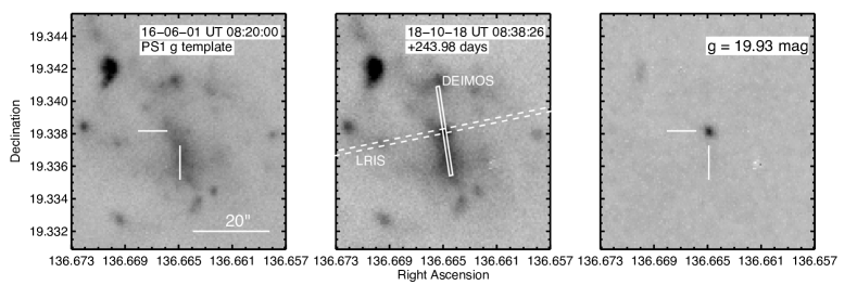
Figure 1: 0.87^′ $\times$ 0.87^′ PS1 $g$-band template (left), $g$-band Swope image centered on SN 2018oh taken $\sim$244 days after $B$-band maximum brightness (center) and the resulting difference image (right). At this time, SN 2018oh had a $g$-band brightness of $19.93\pm 0.02$ mag. The solid and dashed white lines boxes represent the slit length, width and orientation for the DEIMOS and LRIS observations, respectively (note that the LRIS slit length is much larger than the image). The position of the SN, at the PS1 template (left) and the difference image (right), is marked with tick marks, while for the science image (center) is at the intersection of the two slits.

We show a late-time $g$-band image of SN 2018oh and the PS1 $g$-band template image in Figure 1. Our SN 2018oh photometry is presented in Table 1.

Table 1: SN 2018oh late-time photometry.

MJD	Phase	Filter	Brightness
	(Rest-frame days)		(mag)
58407.37	+242.00	$r$	$21.29\pm 0.14$
58409.36	+243.98	$g$	$19.93\pm 0.02$
58424.35	+258.81	$r$	$21.97\pm 0.16$
58424.36	+258.82	$i$	$21.42\pm 0.18$
58441.31	+275.58	$r$	$22.12\pm 0.14$
58441.32	+275.59	$i$	$21.36\pm 0.10$
58441.33	+275.60	$g$	$20.42\pm 0.03$

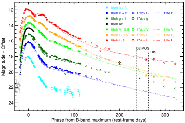
Figure 2: Swope $uBV\!gri$ light curves of SN 2018oh (full circles; offsets noted in the legend) compared to those of SN 2011fe (dotted line) and 2017cbv (open circles), where the light curves of the comparison SNe have been shifted to match the peak of SN 2018oh in each filter. The vertical black dashed lines correspond to the time of our DEIMOS and LRIS spectra, as labeled on the figure. The orange star is our estimate of SN 2018oh’s $r$-band magnitude at 200 days after $B$-band maximum brightness (see Section 3).

Figure 2 displays the complete $uBV\!gri$ Swope light curve of SN 2018oh, spanning from $-7.5$ to +110 days relative to peak $B$ brightness (presented in Li et al. (2018)), with the addition of the new late-time data presented here. The light curves have been corrected for Milky Way extinction using the Fitzpatrick (1999) law (with $R_{V}=3.1$) for $E(B-V)_{MW}=0.037$ mag and placed in rest-frame using $z=0.011$. In a similar manner to Dimitriadis et al. (2018), we compare the light curves of SN 2018oh to those of SNe 2011fe (BV$R_{C}I_{C}$; Munari et al., 2013) and 2017cbv ($BV\!gri$; Rojas-Bravo et al., in prep.). These SNe represent a typical SN Ia with no initial flux excess and a SN Ia with a prominent blue flux excess, respectively. Despite the differences in the first few days after explosion, all three SNe behave similarly, from peak brightness until the epoch of our latest SN 2018oh data.

2.2 Late-time Spectroscopy

We obtained two optical spectra of SN 2018oh: one with the DEep Imaging Multi-Object Spectrograph (DEIMOS; Faber et al., 2003) and one with the Low Resolution Imaging Spectrometer (LRIS; Oke et al., 1995), mounted on the 10-meter Keck II and Keck I telescopes at the W. M. Keck Observatory, respectively. The DEIMOS spectrum consists of two 30-minute exposures, taken on 2018 Oct 10 and 11 (at an average phase of +236.2 days after $B$-band maximum brightness) and covers a (4620 — 9830 Å) wavelength range. We used an 0.8^′′-wide slitlet with the 600ZD grating (central wavelength of 7200 Å) and the GG455 order-blocking filter, with the exposure being taken on the paralactic angle. The data were reduced using a modified version of the DEEP2 data-reduction pipeline (Cooper et al., 2012; Newman et al., 2013), which bias-corrects, flattens, rectifies, and sky-subtracts the data. The LRIS spectrum consists of one 60-minute exposure, taken on 2018 Nov 19 (at an average phase of +264.0 days after $B$-band maximum brightness), and covers a (3300 — 10,100 Å) wavelength range. We used the 1.0^′′-wide slit, the 600/4000 grism (blue side), the 400/8500 grating (red side, central wavelength at 7743 Å) and the D560 dichroic. For that exposure, we used an angle of 170 degrees (north to east), in order to minimize the host-galaxy light contribution, benefiting from the Atmospheric Dispersion Compensator (ADC) module of Keck I, that allows LRIS to operate with reduced differential refraction. These data were reduced using standard iraf for bias corrections and flat fielding. For both of the spectra, we employed our own IDL routines to flux calibrate the data and remove telluric lines using the well-exposed continua of the spectrophotometric standards (e.g., Foley et al., 2003; Silverman et al., 2012).

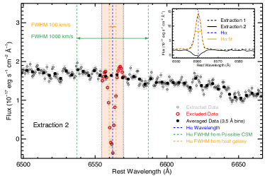
Figure 3: DEIMOS spectrum of SN 2018oh (grey circles) near the position of H$\alpha$. This is our first extracted spectrum where the emission line is oversubtracted. This spectrum and the spectrum resulting from the more distant background regions are shown in the inset (in black and gold, respectively). We fit a Gaussian to the emission feature and display its FWHM as vertical gold-dashed lines. The FWHM of this line is significantly smaller than of a feature expected from swept-up material ($\sim$1000 $\mathrm{km\ s^{-1}}$; indicated by the vertical green-dashed lines). Data within $3\times{\rm FWHM}$ (marked by the vertical black-dotted lines and the peach background) are outlined in red and are removed from our final spectrum. The full black circles correspond to the spectrum with 3.5-Å binning, which we use in Section 3.

Because the SN is embedded in diffuse galactic light, we had to carefully extract the spectra to mitigate host-galaxy contamination. To do this, we extracted the SN spectrum using two sets of background regions. One has the background regions close to the SN position, which provides an excellent representation of the continuum flux at the SN position. However, since these regions have stronger emission flux than at the SN position, strong emission lines are oversubtracted. To compensate for this effect, we also extracted the SN spectrum with the background regions further from the SN position, which does not fully remove the galactic light, but also provides an accurate measurement of the emission flux at the SN position. Using the second extraction that has undersubtracted galactic emission features, we fit a Gaussian to the H$\alpha$ emission line (Figure 3), finding a FWHM of $100\pm 20\ \mathrm{km\ s^{-1}}$. This line is significantly narrower than what is predicted for the interaction scenario ($\sim$1000 $\mathrm{km\ s^{-1}}$), indicating that it originates from the galaxy. We then replace all data within $3\times{\rm FWHM}$ in the first extraction (that originally had oversubtracted features) using a linear fit to the remaining dataset, and finally rebinning the spectrum to 3.5 Å, to obtain our final spectra.

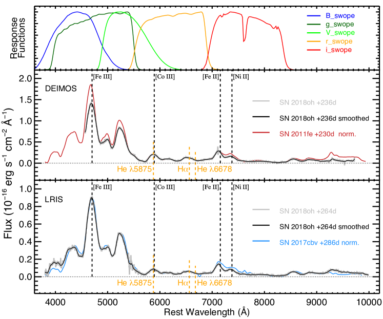
Figure 4: Rest-frame nebular-phase (+236, middle panel, and 264, bottom panel, days form B-band maximum) spectra of SN 2018oh. We show the 3.5Å-binned spectra with grey and the 100Å-smoothed with black solid lines, respectively. We compare the spectra with the +230 days SN 2011fe spectrum (red; Graham et al., 2015) and the +286 days SN 2017cbv spectrum (blue; Sand et al., 2018). All spectra are normalized to the flux of SN 2018oh in the $r$-band of the Swope telescope at its corresponding phase, for which we plot the response functions of its broad-band filters at the top panel. We also mark four iron-peak elements’ nebular-phase lines (vertical dashed black lines) and the three zero-velocity positions of the expected interaction lines from Hydrogen and Helium in the interaction scenario (vertical dashed orange lines).

The nebular spectra of SN 2018oh are shown as the solid grey lines in Figure 4. The spectra have been corrected for Milky-Way reddening with the same Fitzpatrick (1999) law as our photometry, and smoothed using a second-order, 100-Å-wide Savitzky–Golay smoothing polynomial, shown with a solid black line. We additionally overplot two late-time spectra of SNe 2011fe (Graham et al., 2015) and 2017cbv (Sand et al., 2018) at +230 and +286 days respectively, corrected and smoothed in the same manner and scaled to the $r$-band flux of SN 2018oh.

We do not detect any relatively narrow hydrogen or helium emission features originating from swept-up material. We determine the flux limits for these features and mass limits for the material below.

3 Mass Limits For Swept-up Material

In order to provide statistical constraints on the amount of stripped material from a potential non-degenerate companion, we follow the methodology of Sand et al. (2018). This approach is similar to previous works (Shappee et al., 2013; Maguire et al., 2016; Graham et al., 2017; Shappee et al., 2018a), but uses recent multi-dimensional radiative transfer models and hydrodynamical simulations of ejecta-companion interaction from Botyánszki et al. (2018) instead of simpler treatments based on the models of Mattila et al. (2005) and Lundqvist et al. (2013). Botyánszki et al. (2018) uses the Boehner et al. (2017) hydrodynamical models of a SN Ia interacting with its companion and synthesizes the resulting spectra at +200 days after peak.

Despite the Botyánszki et al. (2018) spectrum being generated for an epoch of 200 days after peak and our spectrum being from 230 days after peak, we can still easily compare the data to the models. Since SN Ia spectral features do not change significantly between these two epochs, we can assume that SN 2018oh had the same spectral shape at +200 days as it has in our spectrum. To appropriately scale the flux, we simply interpolate our $r$-band Swope light curve (which wavelength range covers the hydrogen and helium lines we are interested in) to determine the brightness at +200 days, finding $r_{200\mathrm{d}}=20.40\pm 0.23$ mag. Finally, we bin our spectra to 3.5 Å, similar to Sand et al. (2018), so that we can directly compare SN 2018oh to SN 2017cbv. The final DEIMOS spectrum is shown as a black solid line in Figure 5.

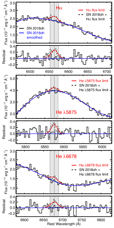
Figure 5: The DEIMOS spectrum of SN 2018oh zoomed in to show H$\alpha$ (top panel), He I $\lambda 5875$ (middle panel), and He I $\lambda 6678$ (bottom panel). The flux is adjusted to what would have been seen 200 days after maximum brightness. The underlying continuum, which we approximate with a Savitsky–-Golay smoothed (with a 180-Å filter) version of the spectrum, is displayed as blue solid lines. The grey-shaded region corresponds the $\pm 22$Å (roughly 1000 $\mathrm{km\ s^{-1}}$) region around the rest wavelength of each line. In red, we insert a feature at the rest-wavelength of each line with a FWHM of 1000 $\mathrm{km\ s^{-1}}$ and a height corresponding to our 3-$\sigma$ detection limit above the smoothed continuum. With a dashed black line, we also show how such a feature would look in the data. For each feature, we also display the residuals relative to the continuum.

As seen in Figure 4, the hydrogen and helium emission lines coincide with broad emission features from the SN. Thus, in order to appropriately determine the continuum of this underlying emission, we use a second-order Savitsky–Golay smoothing polynomial filter with a window of 180 Å. We repeated our analysis with varying window widths (80 to 260 Å), and our final mass estimates are well within 1-$\sigma$ of our initial choice. We will continue our analysis with the 180 Å window width to ease comparison with the Sand et al. (2018) study of SN 2017cbv.

Examining the unsmoothed DEIMOS spectrum, both in isolation and compared to the smoothed spectrum, we detect no obvious emission features expected from the interaction scenario. To determine the flux limit for these features, we first measure the RMS noise in the residual (data-continuum) spectra. We approximate these emissions as Gaussians with a peak flux of 3$\times$RMS, at the spectral region of H$\alpha$, He I $\lambda 5875$, and He I $\lambda 6678$ and a FWHM of 22 Å (corresponding to $1000\ \mathrm{km\ s^{-1}}$). Our nominal 3-$\sigma$ flux limit for H$\alpha$, He I $\lambda 5875$, and He I $\lambda 6678$ are $2.6,\ 2.9\ \mathrm{and}\ 2.1\times 10^{-18}\ \mathrm{erg\ s^{-1}\ cm^{-2}\textup{\AA}^{-1}}$, respectively. Adopting the luminosity distance computed in Li et al. (2018) the luminosity limits are $2.1,\ 2.0\ \mathrm{and}\ 1.6\times 10^{37}\ \mathrm{erg\ s^{-1}}$, respectively, and converting the luminosity limits to mass limits using Equation 1 of Botyánszki et al. (2018), we determine SN 2018oh had maximum stripped hydrogen and helium masses of $5.4\times 10^{-4}\ \mathrm{M_{\odot}}$ and $4.7\times 10^{-4}\ \mathrm{M_{\odot}}$, respectively. By adopting 1-$\sigma$ uncertainties of the SN brightness at 200 days and of the luminosity distance, we estimate flux limits of $3.2,\ 3.5\ \mathrm{and}\ 2.5\times 10^{-18}\ \mathrm{erg\ s^{-1}\ cm^{-2}\textup{\AA}^{-1}}$, luminosity limits of $2.6,\ 2.5\ \mathrm{and}\ 2.1\times 10^{37}\ \mathrm{erg\ s^{-1}}$ and mass limits of $6.4\times 10^{-4}\ \mathrm{M_{\odot}}$ and $5.5\times 10^{-4}\ \mathrm{M_{\odot}}$. We repeated our analysis with our LRIS spectrum, taken at +264 days from maximum, deriving similar mass limits ($M_{H}<6.5\times 10^{-4}\ \mathrm{M_{\odot}}$ and $M_{He}<8.4\times 10^{-4}\ \mathrm{M_{\odot}}$), thus we continue our analysis with the DEIMOS +232 days spectrum.

We additionally provide the mass limit of hydrogen, derived using the method of Leonard (2007), for which the authors use the models from Mattila et al. (2005). Mattila et al. (2005) estimate that, at +380 days from peak brightness, a gaussian emission line of $3.36\times 10^{35}\ \mathrm{erg\ s^{-1}\ \textup{\AA}^{-1}}$ is expected from 0.05 $\mathrm{M_{\odot}}$ of stripped hydrogen. By scaling our DEIMOS spectrum to that epoch, adopting the linear decline rate of a factor of 4 at 200–300 days, we derive an equivalent width of that feature of $W_{\lambda}(0.05\ \mathrm{M_{\odot}})=25.53$ Å, while the equivalent width of the strongest gaussian emission line of our spectrum that could remain undetected, at that region, is $W_{\lambda}(3\sigma)=0.99$ Å. Finally, adopting the linear scale between the mass of hydrogen and the equivalent width of the emission line, we derive the upper mass limit $M_{H}<1.9\times 10^{-3}\ \mathrm{M_{\odot}}$.

4 Discussion and conclusions

We have presented late-time photometry and spectroscopy of the closest SN observed by Kepler, SN 2018oh, which exhibits a prominent early linearly rising light curve, before settling back to a typical $L\propto t^{2}$ rise. Examining the spectrum, we do not detect the relatively narrow emission expected when a SN interacts with a close, non-degenerate companion and sweeps up material from the companion’s outer layers. After flux-calibrating our nebular spectra to Swope photometry, assuming that the companion star is Roche-lobe filling, and using the models of (Botyánszki et al., 2018), we determine 3-$\sigma$ upper limits for the mass of swept-up hydrogen and helium of $5.4\times 10^{-4}\ \mathrm{M_{\odot}}$ and $4.7\times 10^{-4}\ \mathrm{M_{\odot}}$, respectively.

Dimitriadis et al. (2018) consider two possible physical mechanisms that adequately reproduce the early Kepler/K2 light curve: interaction with a companion at a distance of $a=2\times 10^{12}$ cm and $0.03\,$M_⊙ of ⁵⁶Ni in the outer layers of the ejecta. While both of these mechanisms were considered possible, the surface ⁵⁶Ni model cannot easily reproduce the blue color observed in the first few days. Because of the color constraint, Dimitriadis et al. (2018) slightly favored the interaction scenario.

Assuming the Roche-Lobe filling criterion, Dimitriadis et al. (2018) suggests a subgiant companion with $M\approx 1$–6 M_⊙ and $R\approx 10$–15 R_⊙. Botyánszki et al. (2018), using Boehner et al. (2017) models, provide H$\alpha$ luminosities for various companion stars, with the Dimitriadis et al. (2018) proposed companion star having properties intermediate to models MS38, SG, and RG319. These models predict $L_{H_{\alpha}}=6.8$, 5.6 and $4.5\times 10^{39}\ \mathrm{erg\ s^{-1}}$ with $M_{H_{\alpha}}=0.25$, 0.17, and $0.28\ \mathrm{M_{\odot}}$ respectively. For SN 2018oh, the H$\alpha$ luminosity is constrained to be two orders of magnitude less than the models. However, we note that our inferred hydrogen limits are based on the extrapolation of the simulations. Moreover, simulations that cover a wider range of the SD scenario parameter space, such as the binary separation and the companion mass are still lacking.

Our inferred mass limits are in accordance with the recent study of Tucker et al. (2018), where the authors, analyzing a nebular (+265 rest-frame days after maximum) spectrum of SN 2018oh, estimate $M_{H}<6\times 10^{-3}\ \mathrm{M_{\odot}}$ and $M_{He}<2\times 10^{-2}\ \mathrm{M_{\odot}}$.

To date, well–studied SNe Ia with prominent linear-rise components in their early light curves and particularly early blue colors are SNe 2013dy (Zheng et al., 2013), ASASSN-14lp (Shappee et al., 2016), iPTF16abc (Miller et al., 2018), 2017cbv (Hosseinzadeh et al., 2017) and 2018oh (Dimitriadis et al., 2018). However, no SN in this sample has nebular spectra indicative of companion interaction (Shappee et al., 2018a; Sand et al., 2018). There are four possible explanations for the combination of early blue excess flux and a lack of strong, relatively narrow hydrogen and helium emission features in the nebular spectra:

1. SN 2018oh did not have a Roche-Lobe filling companion. However, some SNe Ia clearly have relatively dense CSM as seen by time-variable absorption features (e.g., Patat et al. 2007; Simon et al. 2009 and a relatively large fraction of SNe Ia must be “gas rich;” e.g., Sternberg et al. 2011; Foley et al. 2012b; Maguire et al. 2013), yet those SNe also do not have narrow emission features in their nebular spectra. Furthermore, SNe Iax (Foley et al., 2013) have strong evidence for Roche-lobe filling companions (e.g., McCully et al., 2014), but none have strong hydrogen or helium emission lines in their late-time spectra (Foley et al. 2016; Jacobson-Galán et al., in prep.). There are also some SNe Ia that have strong emission lines from circumstellar interaction, including at early times (the “SN Ia-CSM” class; e.g., Dilday et al., 2012; Silverman et al., 2013), but this emission is exclusively very strong indicating very dense CSM. While SN 2018oh may lack a Roche-lobe filling companion, that alone does not explain the lack of hydrogen/helium emission features in other nebular spectra and the lack of weak interaction signatures for some SNe Ia-CSM.

2. The current theoretical models of the Roche-Lobe filling SD scenario overpredict the H$\alpha$ luminosity at the times of our data. While these theoretical models cannot fully capture the complex physics involved (asymmetries in the explosion, precise atomic line data, reliable radiative transport codes), it is unlikely that the amount of stripped material predicted is off by two orders of magnitude. At face value, this explanation seems unlikely.

3. SN 2018oh had a more distant non-degenerate companion (i.e., a symbiotic progenitor system). Having a more distant companion would reduce the amount of material stripped from its surface. However, one would need a very unlikely orientation to possibly reproduce the early flux.

4. SN 2018oh had a significant amount of ⁵⁶Ni on its surface (to produce the fast rise of the light curve) and radiative transfer calculations incorrectly predict that this light should be red (because of line blanketing from the high abundance of Fe-group elements). Again, simple calculations show that the excess flux produced in this scenario should be red, inconsistent with SN 2018oh. Red flux excesses have been seen for other SNe (Jiang et al., 2017), further indicating that this basic scenario is correct for at least some events. An asymmetric distribution of ⁵⁶Ni in the outermost layers combined with a particular viewing angle may resolve this issue.

5. Some models are able to reproduce the general properties of SN 2018oh, such as a detached system consisting of a WD and a RG-like companion under the common-envelope wind SD scenario (Meng & Podsiadlowski, 2018; Meng & Li, 2018), or a non-violent DD scenario involving the collision of the SN ejecta with circumstellar material originating from an accretion disk formed during the merger process of the two WDs (Levanon & Soker, 2017). However, more detailed modeling of these potentially rare channels, alongside studies involving their rates, is necessary.

Considering several possibilities, we conclude that there are no known models that can simultaneously explain the blue early-time flux excess and the lack of late-time narrow emission lines. As the population of these remarkable events grows, we will be able to statistically investigate their properties which may reveal other possible explanations (e.g. see Stritzinger et al., 2018). In addition to new discoveries and observations, more realistic theoretical models, with better radiative transfer calculations, are needed. We will continue observing SN 2018oh and, at the same time, actively pursue to discover other SNe Ia within hours of explosion, focusing on their early color evolution and spectral evolution from the first few hours to several months after peak brightness.

Swope, Keck:I (LRIS), Keck:II (DEIMOS)

References

- Arnett (1982) Arnett, W. D. 1982, ApJ, 253, 785
- Becker (2015) Becker, A. 2015, HOTPANTS: High Order Transform of PSF ANd Template Subtraction, Astrophysics Source Code Library, , , ascl:1504.004
- Bloom et al. (2012) Bloom, J. S., Kasen, D., Shen, K. J., et al. 2012, ApJ, 744, L17
- Boehner et al. (2017) Boehner, P., Plewa, T., & Langer, N. 2017, MNRAS, 465, 2060
- Botyánszki et al. (2018) Botyánszki, J., Kasen, D., & Plewa, T. 2018, ApJ, 852, L6
- Chambers et al. (2016) Chambers, K. C., Magnier, E. A., Metcalfe, N., et al. 2016, ArXiv e-prints, arXiv:1612.05560
- Colgate & McKee (1969) Colgate, S. A., & McKee, C. 1969, ApJ, 157, 623
- Cooper et al. (2012) Cooper, M. C., Newman, J. A., Davis, M., Finkbeiner, D. P., & Gerke, B. F. 2012, spec2d: DEEP2 DEIMOS Spectral Pipeline, Astrophysics Source Code Library, , , ascl:1203.003
- DES Collaboration et al. (2018) DES Collaboration, Abbott, T. M. C., Allam, S., et al. 2018, ArXiv e-prints, arXiv:1811.02374
- Dilday et al. (2012) Dilday, B., Howell, D. A., Cenko, S. B., et al. 2012, Science, 337, 942
- Dimitriadis et al. (2018) Dimitriadis, G., Foley, R. J., Rest, A., et al. 2018, ArXiv e-prints, arXiv:1811.10061
- Dotson et al. (2018) Dotson, J. L., Rest, A., Barentsen, G., et al. 2018, Research Notes of the American Astronomical Society, 2, 178
- Faber et al. (2003) Faber, S. M., Phillips, A. C., Kibrick, R. I., et al. 2003, in Proc. SPIE, Vol. 4841, Instrument Design and Performance for Optical/Infrared Ground-based Telescopes, ed. M. Iye & A. F. M. Moorwood, 1657–1669
- Firth et al. (2015) Firth, R. E., Sullivan, M., Gal-Yam, A., et al. 2015, MNRAS, 446, 3895
- Fitzpatrick (1999) Fitzpatrick, E. L. 1999, PASP, 111, 63
- Foley et al. (2016) Foley, R. J., Jha, S. W., Pan, Y.-C., et al. 2016, MNRAS, 461, 433
- Foley et al. (2003) Foley, R. J., Papenkova, M. S., Swift, B. J., et al. 2003, PASP, 115, 1220
- Foley et al. (2012a) Foley, R. J., Challis, P. J., Filippenko, A. V., et al. 2012a, ApJ, 744, 38
- Foley et al. (2012b) Foley, R. J., Simon, J. D., Burns, C. R., et al. 2012b, ApJ, 752, 101
- Foley et al. (2013) Foley, R. J., Challis, P. J., Chornock, R., et al. 2013, ApJ, 767, 57
- Ganeshalingam et al. (2011) Ganeshalingam, M., Li, W., & Filippenko, A. V. 2011, MNRAS, 416, 2607
- González-Gaitán et al. (2012) González-Gaitán, S., Conley, A., Bianco, F. B., et al. 2012, ApJ, 745, 44
- Graham et al. (2015) Graham, M. L., Nugent, P. E., Sullivan, M., et al. 2015, MNRAS, 454, 1948
- Graham et al. (2017) Graham, M. L., Kumar, S., Hosseinzadeh, G., et al. 2017, MNRAS, 472, 3437
- Haas et al. (2010) Haas, M. R., Batalha, N. M., Bryson, S. T., et al. 2010, ApJ, 713, L115
- Hayden et al. (2010) Hayden, B. T., Garnavich, P. M., Kessler, R., et al. 2010, ApJ, 712, 350
- Hillebrandt et al. (2013) Hillebrandt, W., Kromer, M., Röpke, F. K., & Ruiter, A. J. 2013, Frontiers of Physics, 8, 116
- Hosseinzadeh et al. (2017) Hosseinzadeh, G., Sand, D. J., Valenti, S., et al. 2017, ApJ, 845, L11
- Hoyle & Fowler (1960) Hoyle, F., & Fowler, W. A. 1960, ApJ, 132, 565
- Iben & Tutukov (1984) Iben, Jr., I., & Tutukov, A. V. 1984, ApJS, 54, 335
- Jiang et al. (2017) Jiang, J.-A., Doi, M., Maeda, K., et al. 2017, Nature, 550, 80
- Jones et al. (2018) Jones, D. O., Scolnic, D. M., Riess, A. G., et al. 2018, ApJ, 857, 51
- Kasen (2010) Kasen, D. 2010, ApJ, 708, 1025
- Kasen et al. (2009) Kasen, D., Röpke, F. K., & Woosley, S. E. 2009, Nature, 460, 869
- Leadbeater (2018) Leadbeater, R. 2018, Transient Name Server Classification Report, 159
- Leonard (2007) Leonard, D. C. 2007, ApJ, 670, 1275
- Levanon & Soker (2017) Levanon, N., & Soker, N. 2017, MNRAS, 470, 2510
- Li et al. (2018) Li, W., Wang, X., Vinkó, J., et al. 2018, ArXiv e-prints, arXiv:1811.10056
- Liu et al. (2013) Liu, Z.-W., Pakmor, R., Seitenzahl, I. R., et al. 2013, ApJ, 774, 37
- Lundqvist et al. (2013) Lundqvist, P., Mattila, S., Sollerman, J., et al. 2013, MNRAS, 435, 329
- Magnier et al. (2016) Magnier, E. A., Chambers, K. C., Flewelling, H. A., et al. 2016, ArXiv e-prints, arXiv:1612.05240
- Maguire et al. (2016) Maguire, K., Taubenberger, S., Sullivan, M., & Mazzali, P. A. 2016, MNRAS, 457, 3254
- Maguire et al. (2013) Maguire, K., Sullivan, M., Patat, F., et al. 2013, MNRAS, 436, 222
- Marietta et al. (2000) Marietta, E., Burrows, A., & Fryxell, B. 2000, ApJS, 128, 615
- Marion et al. (2016) Marion, G. H., Brown, P. J., Vinkó, J., et al. 2016, ApJ, 820, 92
- Mattila et al. (2005) Mattila, S., Lundqvist, P., Sollerman, J., et al. 2005, A&A, 443, 649
- McCully et al. (2014) McCully, C., Jha, S. W., Foley, R. J., et al. 2014, Nature, 512, 54
- Meng & Li (2018) Meng, X., & Li, J. 2018, arXiv e-prints, arXiv:1811.11351
- Meng & Podsiadlowski (2018) Meng, X., & Podsiadlowski, P. 2018, ApJ, 861, 127
- Miller et al. (2018) Miller, A. A., Cao, Y., Piro, A. L., et al. 2018, ApJ, 852, 100
- Munari et al. (2013) Munari, U., Henden, A., Belligoli, R., et al. 2013, New A, 20, 30
- Newman et al. (2013) Newman, J. A., Cooper, M. C., Davis, M., et al. 2013, ApJS, 208, 5
- Nugent et al. (2011) Nugent, P. E., Sullivan, M., Cenko, S. B., et al. 2011, Nature, 480, 344
- Oke et al. (1995) Oke, J. B., Cohen, J. G., Carr, M., et al. 1995, PASP, 107, 375
- Olling et al. (2015) Olling, R. P., Mushotzky, R., Shaya, E. J., et al. 2015, Nature, 521, 332
- Pan et al. (2012) Pan, K.-C., Ricker, P. M., & Taam, R. E. 2012, ApJ, 750, 151
- Patat et al. (2007) Patat, F., Chandra, P., Chevalier, R., et al. 2007, Science, 317, 924
- Rest et al. (2005) Rest, A., Stubbs, C., Becker, A. C., et al. 2005, ApJ, 634, 1103
- Rest et al. (2014) Rest, A., Scolnic, D., Foley, R. J., et al. 2014, ApJ, 795, 44
- Riess et al. (1999) Riess, A. G., Filippenko, A. V., Li, W., et al. 1999, AJ, 118, 2675
- Riess et al. (2016) Riess, A. G., Macri, L. M., Hoffmann, S. L., et al. 2016, ApJ, 826, 56
- Sand et al. (2018) Sand, D. J., Graham, M. L., Botyánszki, J., et al. 2018, ApJ, 863, 24
- Schechter et al. (1993) Schechter, P. L., Mateo, M., & Saha, A. 1993, PASP, 105, 1342
- Scolnic et al. (2018) Scolnic, D. M., Jones, D. O., Rest, A., et al. 2018, ApJ, 859, 101
- Shappee et al. (2018a) Shappee, B. J., Piro, A. L., Stanek, K. Z., et al. 2018a, ApJ, 855, 6
- Shappee et al. (2013) Shappee, B. J., Stanek, K. Z., Pogge, R. W., & Garnavich, P. M. 2013, ApJ, 762, L5
- Shappee et al. (2014) Shappee, B. J., Prieto, J. L., Grupe, D., et al. 2014, ApJ, 788, 48
- Shappee et al. (2016) Shappee, B. J., Piro, A. L., Holoien, T. W.-S., et al. 2016, ApJ, 826, 144
- Shappee et al. (2018b) Shappee, B. J., Holoien, T. W.-s., Drout, M. R., et al. 2018b, ArXiv e-prints, arXiv:1807.11526
- Silverman et al. (2012) Silverman, J. M., Foley, R. J., Filippenko, A. V., et al. 2012, MNRAS, 425, 1789
- Silverman et al. (2013) Silverman, J. M., Nugent, P. E., Gal-Yam, A., et al. 2013, ApJS, 207, 3
- Sim et al. (2013) Sim, S. A., Seitenzahl, I. R., Kromer, M., et al. 2013, MNRAS, 436, 333
- Simon et al. (2009) Simon, J. D., Gal-Yam, A., Gnat, O., et al. 2009, ApJ, 702, 1157
- Sternberg et al. (2011) Sternberg, A., Gal-Yam, A., Simon, J. D., et al. 2011, Science, 333, 856
- Stritzinger et al. (2018) Stritzinger, M. D., Shappee, B. J., Piro, A. L., et al. 2018, ApJ, 864, L35
- Tucker et al. (2018) Tucker, M. A., Shappee, B. J., & Wisniewski, J. P. 2018, arXiv e-prints, arXiv:1811.09635
- Waters et al. (2016) Waters, C. Z., Magnier, E. A., Price, P. A., et al. 2016, ArXiv e-prints, arXiv:1612.05245
- Whelan & Iben (1973) Whelan, J., & Iben, Jr., I. 1973, ApJ, 186, 1007
- Woosley & Kasen (2011) Woosley, S. E., & Kasen, D. 2011, ApJ, 734, 38
- Woosley et al. (1986) Woosley, S. E., Taam, R. E., & Weaver, T. A. 1986, ApJ, 301, 601
- Zhang et al. (2018) Zhang, J., Xin, Y., Li, W., et al. 2018, The Astronomer’s Telegram, 11267
- Zheng et al. (2013) Zheng, W., Silverman, J. M., Filippenko, A. V., et al. 2013, ApJ, 778, L15